Modelling cancer progression using Mutual Hazard Networks

Abstract

Motivation

Cancer progresses by accumulating genomic events, such as mutations and copy number alterations, whose chronological order is key to understanding the disease but difficult to observe. Instead, cancer progression models use co-occurrence patterns in cross-sectional data to infer epistatic interactions between events and thereby uncover their most likely order of occurrence. State-of-the-art progression models, however, are limited by mathematical tractability and only allow events to interact in directed acyclic graphs, to promote but not inhibit subsequent events, or to be mutually exclusive in distinct groups that cannot overlap.

Results

Here we propose Mutual Hazard Networks (MHN), a new Machine Learning algorithm to infer cyclic progression models from cross-sectional data. MHN model events by their spontaneous rate of fixation and by multiplicative effects they exert on the rates of successive events. MHN compared favourably to acyclic models in cross-validated model fit on four datasets tested. In application to the glioblastoma dataset from The Cancer Genome Atlas, MHN proposed a novel interaction in line with consecutive biopsies: IDH1 mutations are early events that promote subsequent fixation of TP53 mutations.

Availability and implementation

Implementation and data are available at https://github.com/RudiSchill/MHN.

Supplementary information

Supplementary data are available at Bioinformatics online.

1 Introduction

Tumours turn malignant in a Darwinian evolutionary process by accumulating genetic mutations, copy number alterations, changes in DNA methylation, gene expression and protein concentration. Such progression events arise in individual tumour cells, but their effect on the reproductive fitness of this cell depends on earlier events (Nowell, 1976), which makes some chronological sequences of alterations more likely than others. These sequences and their driving dependencies are a priori unknown and inferring them from data is the goal of cancer progression models. These roughly fall into three classes: phylogenetic models, models of population dynamics and cross-sectional models (Beerenwinkel et al., 2015; Schwartz and Schäffer, 2017). We focus on the latter.

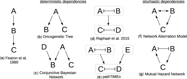
While progression is a dynamic process, available genotype data are cross-sectional and combine static snapshots from different tumours at different stages of development. Nevertheless, assuming that the tumour genomes are observations from the same stochastic process, cancer progression models can infer dependencies between events from their co-occurrence patterns. The dependencies are then reported as a directed graph, where each node stands for an event whose probability depends in some way on the events connected to it by incoming edges (Fig. 1).

Fig. 1.

Overview of several types of cancer progression models. For models with deterministic dependencies (a-e) $A\to B$ denotes that A is necessary for B, and $A⊣B$ denotes that A prevents B. For models with stochastic dependencies (f,g) $A\to B$ denotes that A makes B more likely, and $A⊣B$ denotes that A makes B less likely. In (d-e) the arrows between groups of events denote that at least one of the events in the parent group is necessary for the events in the child group

For example, one family of models [reviewed by Hainke et al. (2012)] approximate tumour progression by deterministic dependencies: An event has a non-zero probability if and only if all its parent events have occurred. These models were inspired by Fearon and Vogelstein (1990), who inferred that colorectal cancers progress along a chain of mutations in the genes APC → K-RAS → TP53. Desper et al. (1999) formalized and extended this concept to Oncogenetic Trees, where a single event may be necessary for multiple successor events in parallel. Beerenwinkel et al. (2007) further generalized these to Conjunctive Bayesian Networks (CBN), where events may require multiple precursors, thus replacing trees by directed acyclic graphs.

In this paper, we relax three assumptions of this model family:

1. Dependencies need not be deterministic. An event A can make an event B more likely without being absolutely necessary for it. In particular, events can occur with non-zero probability at all times and all event patterns are possible.

2. A dependency graph need not be acyclic. Why should it? Clearly an event A cannot be necessary for B if B is also necessary for A. But it is certainly possible that A makes B more likely when it occurs first, and vice versa.

3. Besides enabling dependencies, there are also inhibiting dependencies.

Although there is, to the best our knowledge, no method that addresses all three issues, there are methods that address one or two of them. Stochastic dependencies (1) have been previously proposed in Farahani and Lagergren (2013), Misra et al. (2014) and Ramazzotti et al. (2015) for acyclic models. Moreover, stochasticity at the point of observation has been addressed by Gerstung et al. (2011) who allow for mislabeled events, and in Beerenwinkel et al. (2005) and Montazeri et al. (2016) who treat tumour data as a mixture from multiple stochastic processes. Network Aberration Models (NAM) by Hjelm et al. (2006) have stochastic dependencies (1) and allow cycles in their dependency graph (2).

Inhibition (3) is at the centre of mutual exclusivity, which is a frequently observed phenomenon in cancer (Yeang et al., 2008). Two events are considered mutually exclusive if they co-occur less frequently than expected by chance. There are at least two mechanisms that can cause this data pattern: (i) Synthetic lethality, where cells carrying two mutations A and B are no longer vital. (ii) The events disrupt the same molecular pathway such that whichever event occurs first conveys most of the selective advantage and decreases selective pressure for the others. Both mechanisms can be described by a double edge A $⊢⊣$ B (A inhibits B, and B inhibits A)

Gerstung et al. (2011) proposed to model pathways within a progression model from biological prior knowledge. They extracted predefined sets of events from databases reflecting biological pathways which are considered affected if at least one of its constituent events has occurred. Tumour progression is then modelled on the level of pathways rather than events.

Alternatively pathways can be derived from data by detecting patterns of mutual exclusivity (Constantinescu et al., 2015; Leiserson et al., 2013; Miller et al., 2011; Szczurek and Beerenwinkel, 2014) or by a combination of knowledge and data (Ciriello et al., 2012; Kim et al., 2015), see (Vandin, 2017) for a review. Raphael and Vandin (2015) pointed out that inferring pathways separately from their dependencies can lead to inconsistencies in the presence of noise. They presented the first algorithm that simultaneously groups events into pathways and arranges the pathways in a linear chain. PathTiMEx (Cristea et al., 2017) generalizes this from linear chains to acyclic progression networks (CBN).

Building on both CBNs and NAMs, we propose Mutual Hazard Networks (MHN). MHNs do not group events into pathways but directly model the mechanisms behind mutual exclusivity. MHNs have cyclic dependency networks, in particular allowing for bidirectional and inhibiting edges.

MHN characterize events by a baseline rate and by multiplicative effects they exert on the rates of successive events. These effects can be greater or less than one, i.e. promoting or inhibiting. We provide formulas for the log-likelihood of MHN and its gradient, and an implementation that is computationally tractable for systems with up to 25 events on a standard workstation and for larger systems on an HPC infrastructure.

2 Materials and methods

2.1 Mutual Hazard Networks

We model tumour progression as a continuous time Markov process $\left\{X\left(t\right),t\ge 0\right\}$ on all $2^n$ combinations of a predefined set of n events. Its state space is $S={\left\{0,1\right\}}^n$, where $X{\left(t\right)}_i=1$ means that event i has occurred in the tumour by age t, while $X{\left(t\right)}_i=0$ means that it has not.

We assume that every progression trajectory starts at a normal genome $X\left(0\right)={(0,\dots ,0)}^T$, accumulates irreversible events one at a time, and ends at a fully aberrant genome $X(\infty )={(1,\dots ,1)}^T$. Observed tumour genomes correspond to states at unknown intermediate ages $0<t<\infty$ and typically hold both 0 and 1 entries.

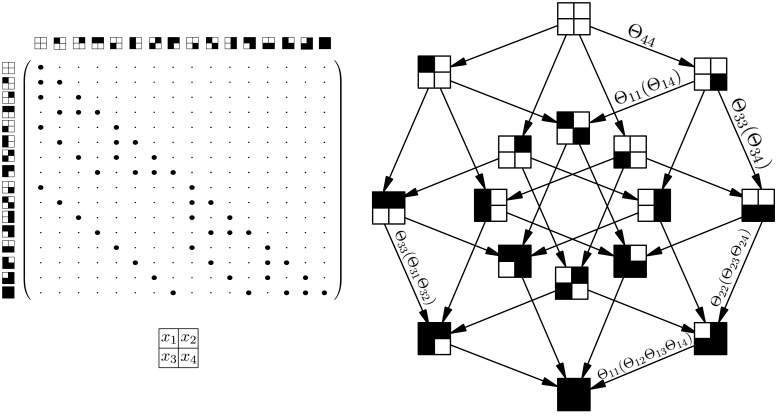
Let $Q\in {\mathbb{R}}^{2^n\times 2^n}$ be the transition rate matrix of this process with respect to a basis of S in lexicographic order (Fig. 2, left). An entry

$$Q_{\mathbf{y},\mathbf{x}}=\underset{\Delta t\to 0}{\lim }\frac{\mathrm{Pr}\left(X(t+\Delta t)=\mathbf{y}\left|X\right(t)=\mathbf{x}\right)}{\Delta t},\hspace{1em}\mathbf{y}\ne \mathbf{x}$$ (1)

is the rate from state $\mathbf{x}\in S$ to state $\mathbf{y}\in S$, and diagonal elements are defined as $Q_{\mathbf{x},\mathbf{x}}=-\sum _{\mathbf{y}\ne \mathbf{x}}{Q}_{\mathbf{y},\mathbf{x}}$ so that columns sum to zero. Q is lower triangular and has non-zero entries only for transitions between pairs of states $\mathbf{x}={(\dots ,x_{i-1},0,x_{i+1},\dots )}^T$ and $\mathbf{y}={\mathbf{x}}_{+i}:={(\dots ,x_{i-1},1,x_{i+1},\dots )}^T$ that differ in a single entry i.

Fig. 2.

(Left) Transition rate matrix Q for the Markov process X with n = 4, where $·$ is a zero entry and $•$ is a non-zero entry. The states are depicted as squares with four compartments as shown below. A white compartment denotes 0 and a black compartment denotes 1. The matrix is lower triangular because events are irreversible, and sparse because events accumulate one at a time. (Right) Parameterization $Q_{\Theta }$ of the Markov process by a Mutual Hazard Network

Our aim is to learn for each event i how its rate $Q_{{\mathbf{x}}_{+i},\mathbf{x}}$ depends on already present events in x as a function $f_i:{\left\{0,1\right\}}^n\to \mathbb{R}$. A common choice in time-to-event analysis is the proportional hazards model (Cox, 1972) which assumes that binary predictors have independent and multiplicative effects on the rate of the event. We therefore specify the Markov process by a system of n functions

$$Q_{{\mathbf{x}}_{+i},\mathbf{x}}=f_i\left(\mathbf{x}\right)=\text{exp}\hspace{0.17em}\left({\theta }_{\mathit{ii}}+\sum _{j=1}^n{\theta }_{\mathit{ij}}{x}_j\right)={\Theta }_{\mathit{ii}}\prod _{x_j=1}{\Theta }_{\mathit{ij}}\hspace{0.17em}$$ (2)

and collect their parameters in a matrix $\left({\Theta }_{\mathit{ij}}\right):=\left(e^{{\theta }_{\mathit{ij}}}\right)\in {\mathbb{R}}^{n\times n}$. We call Θ a Mutual Hazard Network (MHN), where the baseline hazard Θ_ii is the rate of the event i before any other events are present and the hazard ratio Θ_ij is the multiplicative effect of event j on the rate of event i (Fig. 2, right). Note that while the baseline hazard in Cox (1972) is generally a function of time, here it must be constant so that our model constitutes a Markov process.

2.2 Parameter estimation

A dataset $\mathcal{D}$ of tumours defines an empirical probability distribution on S. It can be represented by a vector ${\mathbf{p}}_{\mathcal{D}}$ of size $2^n$, where an entry ${\left({\mathbf{p}}_{\mathcal{D}}\right)}_{\mathbf{x}}$ is the relative frequency of observed tumours with state x in $\mathcal{D}$.

At t = 0 tumours are free of any events, so the Markov process X starts with the initial distribution ${\mathbf{p}}_{\varnothing }:={(100\%,0\%,\dots ,0\%)}^T$, which then evolves according to the parameterized rate matrix $Q_{\Theta }$. If all tumours had been observed at a common age t, ${\mathbf{p}}_{\mathcal{D}}$ could be modelled as a sample from the transient distribution

$$e^{t{Q}_{\Theta }}{\mathbf{p}}_{\varnothing }.$$ (3)

Since the tumour age is usually unknown, we follow Gerstung et al. (2009) and consider t to be an exponential random variable with mean 1. Marginalizing over t yields

$${\mathbf{p}}_{\Theta }={\int }_0^{\infty }dt{e}^{-t}{e}^{t{Q}_{\Theta }}{\mathbf{p}}_{\varnothing }={\underset{=:R_{\Theta }}{\underbrace{[I-Q_{\Theta }]}}}^{-1}{\mathbf{p}}_{\varnothing },$$ (4)

and the marginal log-likelihood score of Θ given $\mathcal{D}$ is

$${\mathcal{S}}_{\mathcal{D}}(\Theta )={\mathbf{p}}_{\mathcal{D}}^T\hspace{0.17em}\text{log}\hspace{0.17em}{\mathbf{p}}_{\Theta }={\mathbf{p}}_{\mathcal{D}}^T\hspace{0.17em}\text{log}\left(R_{\Theta }^{-1}{\mathbf{p}}_{\varnothing }\right),$$ (5)

where the logarithm of a vector is taken component-wise.

When optimizing ${\mathcal{S}}_{\mathcal{D}}$ with respect to Θ we further add an L1 penalty in order to control for model complexity and to avoid overfitting. This promotes sparsity of the networks, such that many events do not interact and off-diagonal entries Θ_ij are exactly 1:

$${\mathcal{S}}_{\mathcal{D}}(\Theta )-\lambda \sum _{i\ne j}|\hspace{0.17em}\text{log}\hspace{0.17em}{\Theta }_{\mathit{ij}}|,$$ (6)

where λ is a tuning parameter. We will optimize this expression using the Orthant-Wise Limited-Memory Quasi-Newton algorithm (Andrew and Gao, 2007). This general-purpose optimizer handles the non-differentiable regularization term by approximating the objective at each iteration with a quadratic function that is valid within an orthant of the current set of (logarithmic) parameters. It requires only a closed form for the derivatives $\partial {\mathcal{S}}_{\mathcal{D}}/\partial {\Theta }_{\mathit{ij}}$ with respect to each parameter.

From the chain rule of matrix calculus we have

$$\begin{array}{l}\begin{array}{cc}\frac{\partial {\mathcal{S}}_{\mathcal{D}}}{\partial {\Theta }_{\mathit{ij}}}& =\frac{\partial {\mathcal{S}}_{\mathcal{D}}}{\partial R_{\Theta }^{-1}}·\frac{\partial R_{\Theta }^{-1}}{\partial {\Theta }_{\mathit{ij}}}\end{array}\\ \begin{array}{cc}& =\frac{{\mathbf{p}}_{\mathcal{D}}}{{\mathbf{p}}_{\Theta }}{\mathbf{p}}_{\varnothing }^T·\left(-R_{\Theta }^{-1}\frac{\partial R_{\Theta }}{\partial {\Theta }_{\mathit{ij}}}{R}_{\Theta }^{-1}\right)\end{array}\\ \begin{array}{cc}\hfill & =-{\left(\frac{{\mathbf{p}}_{\mathcal{D}}}{{\mathbf{p}}_{\Theta }}\right)}^T{R}_{\Theta }^{-1}\frac{\partial R_{\Theta }}{\partial {\Theta }_{\mathit{ij}}}{R}_{\Theta }^{-1}{\mathbf{p}}_{\varnothing },\hfill \end{array}\end{array}$$ (7)

where $·$ is the Frobenius product and the ratio ${\mathbf{p}}_{\mathcal{D}}/{\mathbf{p}}_{\Theta }$ is computed component-wise.

In general this optimization converges to one local optimum out of possibly several depending on the starting point. In this paper we always report the optimum reached from an independence model, where the baseline hazard Θ_ii of each event was set to its empirical odds and the hazard ratios were set to exactly 1.

2.3 Efficient implementation

To compute the score in equation (5) and its gradient in equation (7) we must solve the exponentially sized linear systems ${\left[I-Q_{\Theta }\right]}^{-1}{\mathbf{p}}_{\varnothing }$ and ${\left({\mathbf{p}}_{\mathcal{D}}/{\mathbf{p}}_{\Theta }\right)}^T{\left[I-Q_{\Theta }\right]}^{-1}$. To this end, we employ the (left) Kronecker product which is defined for matrices $A\in {\mathbb{R}}^{k\times l}$ and $B\in {\mathbb{R}}^{p\times q}$ as the block matrix

$$A\otimes B=\left[\begin{array}{ccc}{b}_{11}A& \cdots & b_{1l}A\\ ⋮& \ddots & ⋮\\ b_{k1}A& \cdots & b_{\mathit{kl}}A\end{array}\right]\in {\mathbb{R}}^{\mathit{kp}\times \mathit{lq}}.$$ (8)

We follow the literature on structured analysis of large Markov chains (Amoia et al., 1981; Buchholz, 1999) and write the transition rate matrix $Q_{\Theta }$ as a sum of n such Kronecker products,

$$Q_{\Theta }=\sum _{i=1}^n\left[\underset{j<i}{\otimes }\left(\begin{array}{cc}1& 0\\ 0& {\Theta }_{\mathit{ij}}\end{array}\right)\otimes \left(\begin{array}{cc}-{\Theta }_{\mathit{ii}}& 0\\ {\Theta }_{\mathit{ii}}& 0\end{array}\right)\otimes \underset{j>i}{\otimes }\left(\begin{array}{cc}1& 0\\ 0& {\Theta }_{\mathit{ij}}\end{array}\right)\right].$$ (9)

Here, the ith term in the sum is a sparse $2^n\times 2^n$ matrix consisting of all transitions that introduce event i to the genome. It corresponds to a single subdiagonal of $Q_{\Theta }$, together with a negative copy on the diagonal to ensure that columns sum to zero (see Supplementary Section S2). The benefit of this compact representation is that matrix-vector products can be computed in $\mathcal{O}\left(n{2}^{n-1}\right)$ rather than $\mathcal{O}\left(2^{2n}\right)$ without holding the matrix explicitly in memory (Buis and Dyksen, 1996). We split $R_{\Theta }=I-Q_{\Theta }$ into a diagonal and strictly lower triangular part,

$$R_{\Theta }=D+L=D(I+D^{-1}L),$$ (10)

and use the nilpotency of $D^{-1}L$ to compute

$$\begin{array}{c}{R}_{\Theta }^{-1}{\mathbf{p}}_{\varnothing }={(I+D^{-1}L)}^{-1}{D}^{-1}{\mathbf{p}}_{\varnothing }\\ =\left(\sum _{k=0}^{n-1}{(-D^{-1}L)}^k\right)D^{-1}{\mathbf{p}}_{\varnothing }.\end{array}$$ (11)

3 Results

3.1 Simulations

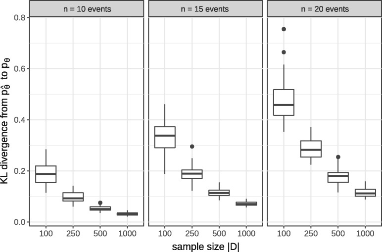
We tested in simulation experiments how well an MHN of a given size can learn a probability distribution on S when trained on a given amount of data. We ran 50 simulations for each of several sample sizes $\left|\mathcal{D}\right|\in \{100,250,500,1000\}$ and number of events $n\in \{10,15,20\}$.

In each simulation run, we chose a ground truth model Θ with n possible events. A random half of its off-diagonal entries were set to 1 (no dependency) and the remaining off-diagonal entries were drawn from a standard log-normal distribution. For the diagonal entries we chose the largest n out of 20 rates drawn from a log-normal distribution with mean $\mu =-2$ and variance ${\sigma }^2=1$. This was done to mimick the event frequencies observed in the biological datasets in Section 3.2 and yielded on average 2.7, 3.5 and 3.9 realized events in tumours with $n\in \{10,15,20\}$ possible events.

We then generated a dataset of size $\left|\mathcal{D}\right|$ from each model and trained on it another model $\widehat{\Theta }$ by optimizing expression (6). We chose a common regularization parameter for all 50 simulation runs, which we found to be roughly $\lambda =1/\left|\mathcal{D}\right|$ through validation on separate datasets of each sample size. We then assessed the reconstructed model $\widehat{\Theta }$ by the Kullback-Leibler (KL) divergence from its probability distribution to the distribution of the true model Θ,

$$D_{\text{KL}}({\mathbf{p}}_{\Theta }\Vert {\mathbf{p}}_{\widehat{\Theta }})={\mathbf{p}}_{\Theta }^T\hspace{0.17em}\text{log}\hspace{0.17em}{\mathbf{p}}_{\Theta }-{\mathbf{p}}_{\Theta }^T\hspace{0.17em}\text{log}\hspace{0.17em}{\mathbf{p}}_{\widehat{\Theta }}.$$ (12)

The median KL divergence, as well as its variance over the 50 simulation runs, improved with larger training datasets and reached almost zero (Fig. 3).

Fig. 3.

KL divergence from estimated MHNs to ground truth MHNs over 50 simulations for the shown sample sizes and number of events

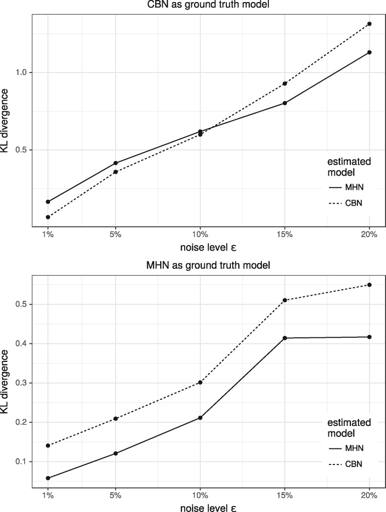
Next, we simulated datasets of size $\left|\mathcal{D}\right|=500$ from random MHNs and CBNs as ground truth models with n = 8 events. We added noise by flipping each event independently with probability ϵ, trained MHNs and CBNs on both datasets and evaluated how well the estimated models fit the distribution of the ground truth models. (Fig. 4) shows the average KL divergence over 5 simulation runs for each noise level $ϵ\in \{1\%,5\%,10\%,15\%,20\%\}$. For CBNs as ground truth we found that CBNs outperformed MHNs when noise was below 10%, while MHNs performed better than CBNs at higher levels of noise. For MHNs as ground truth we found that MHNs performed better than CBNs at all levels of noise.

Fig. 4.

Average KL divergence from estimated MHNs/CBNs to ground truth MHNs/CBNs over 5 simulations for each of the shown noise levels

Lastly, we tested the performance of our implementation. The runtime of a single gradient step for random and dense Θ was about 1 min for n = 20 on a standard workstation and scaled exponentially with n as expected (see Supplementary Section S2 for details).

3.2 Application to cancer progression data

3.2.1 Comparison to conjunctive Bayesian Networks

We tested our method and first compared it to Conjunctive Bayesian Networks (CBN) on three cancer datasets that were previously used by Gerstung et al. (2009). They were obtained from the Progenetix molecular-cytogenetic database (Baudis and Cleary, 2001) and consist of 817 breast cancers, 570 colorectal cancers, and 251 renal cell carcinomas. The cancers are characterized by 10, 11 and 12 recurrent copy number alterations, respectively, which were detected by comparative genomic hybridization (CGH). On average 3.3, 3.5 and 2.6 of these possible events were observed in individual tumours within each dataset.

We trained MHNs on all three datasets (see Supplementary Section S3) and compared them to the CBNs given in Gerstung et al. (2009) which provide log-likelihood scores in-sample. The in-sample scores of MHNs are not directly comparable because MHNs have more degrees of freedom than CBNs. Therefore we additionally provide the average log-likelihood scores of MHNs in 5-fold cross-validation and the Akaike Information Criterion (Akaike, 1974) (AIC) for both models. MHN compared favourably on all three datasets (Table 1).

Table 1.

MHNs compare favourably to CBNs on three datasets in terms of the log-likelihood scores per tumour, averaged over 5 folds in cross-validation

	Cross-validated	In-sample		AIC
Dataset	MHN	CBN	MHN	CBN	MHN
Breast cancer	−5.63	−5.73	−5.54	$\ge$9373	9152
Colorectal cancer	−5.64	−5.79	−5.41	$\ge$6612	6288
Renal cell carcinoma	−5.02	−5.13	−4.81	$\ge$2587	2559

Note: They also compare favourably in terms of the AIC which penalizes the number of parameters in a model and is weighted by the sample size. While MHNs have n² continuous parameters, CBNs have n continuous parameters and a discrete graph structure that is hard to quantify in terms of degrees of freedom, hence we ignore the latter and bound the AIC of CBNs from below.

3.2.2 Comparison to pathTiMEx

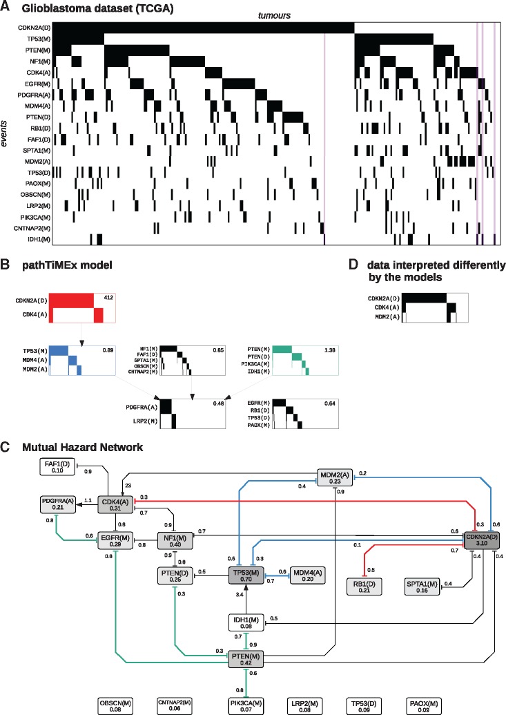
Next, we compared MHN to pathTiMEx on a glioblastoma dataset from The Cancer Genome Atlas (Cerami et al., 2012) which was previously used in Cristea et al. (2017) (see Fig. 5). The data consist of $\left|\mathcal{D}\right|=261$ tumours characterized by 486 point mutations (M), amplifications (A), or deletions (D). We focus on n = 20 of these events which were pre-selected by pathTiMEx using the TiMEx algorithm (Constantinescu et al., 2016). On average 3.3 of these possible events were observed in individual tumours.

Fig. 5.

(A) Glioblastoma dataset from TCGA, where rows show events sorted by frequency and columns show tumours sorted lexicographically. The purple stripes highlight tumours which have IDH1(M) but lack TP53(M). (B) PathTiMEx model inferred in Cristea et al. (2017). It simultaneously divides the dataset into pathways, i.e. into mutually exclusive groups of events and learns a CBN of these pathways. The CBN considers a pathway altered if at least one of its constituent events has occurred. A pathway alteration fixates at the rate given in the upper right-hand corner once all its parent pathways in the CBN have been altered. (C) Mutual Hazard Network, where nodes show the base rates Θ_ii and edges show the multiplicative interactions Θ_ij. Similarities to pathTiMEx are highlighted in colour and roughly correspond to the signaling pathways Rb, p53 and PI(3)K (red, blue and green). (D) Highlighted data interpreted differently by the models. While both models explain the anti-correlation between CDKN2A(D) and CDK4(A) by mutual inhibition, pathTiMEx treats these as a group and infers a positive effect of any of these events on MDM2(A) from the correlation between CDK4(A) and MDM2(A). MHN reports only a positive effect of MDM2(A) on CDK4(A) and in fact infers inhibition between CDKN2A(D) and MDM2(A) from their anti-correlation in the data

We trained MHN as above for 100 iterations, which achieved a log-likelihood score of -7.70 in-sample and a score of -7.97 in 5-fold cross-validation. While pathTiMEx does not yield a directly comparable log-likelihood score, it quantifies discrepancies between model and data by considering the data to be corrupted by noise, each event in a tumour being independently flipped with probability ε. PathTiMEx estimated this noise parameter as $\widehat{\epsilon }=20\%$, from which we gauge an upper bound on its log-likelihood score as follows: even a hypothetical model that learns the data distribution ${\mathbf{p}}_{\mathcal{D}}$ perfectly but assumes a level of noise

$${\mathbf{p}}_{\widehat{\epsilon }}={\otimes }_{i=1}^n\left(\begin{array}{cc}1-\widehat{\epsilon }& \widehat{\epsilon }\\ \widehat{\epsilon }& 1-\widehat{\epsilon }\end{array}\right){\mathbf{p}}_{\mathcal{D}}$$ (13)

achieves only a score of ${\mathbf{p}}_{\mathcal{D}}^T\hspace{0.17em}\text{log}\hspace{0.17em}{\mathbf{p}}_{\widehat{\epsilon }}=-8.50$ in-sample, which is less than the cross-validated score of MHN.

Nevertheless MHN largely agreed with pathTiMEx on the inhibitions implied by the three most mutually exclusive groups of events, which broadly correspond to the signaling pathways Rb, p53 and PI(3)K (red, blue and green in Fig. 5) and are well known to be affected in glioblastoma (McLendon et al., 2008).

The RB1 signaling pathway (red) regulates cell cycle progression and involves the genes CDKN2A, CDK4 and RB1. CDKN2A codes for the tumour suppressor protein p16^INK4a which binds to CDK4 and prevents it from phosphorylizing RB1, thereby blocking cell cycle transition from G1 to S-phase. This function can be disrupted by deletion of CDKN2A or RB1, or by amplification of CDK4. MHN and pathTiMEx both report a corresponding inhibition between the events CDKN2A(D) and CDK4(A), while MHN additionally reports inhibition between CDKN2A(D) and RB1(D).

The p53 signaling pathway (blue) induces apoptosis in response to stress signals and involves the genes TP53, MDM2, MDM4 and CDKN2A. TP53 codes for the tumour suppressor protein p53 which is antagonized by MDM2 and MDM4 in a non-redundant manner (Toledo and Wahl, 2007). PathTiMEx identifies the events TP53(M), MDM2(A), MDM4(A) as mutually exclusive ways to evade apoptosis, while MHN reports inhibition only between TP53(M) and each of MDM2(A) and MDM4(A) separately. This may reflect non-diminishing returns due to their complementary roles in the pathway.

The gene CDKN2A is, in addition to its role in the RB1 pathway, also involved in the p53 pathway by coding for the protein p14^ARF in an alternate reading frame. p14^ARF physiologically inhibits MDM2, which suggests that a deletion of CDKN2A may be functionally similar to an amplification of MDM2. While MHN reports a corresponding inhibition between CDKN2A(D) and MDM2(A), pathTiMEx cannot because this would lead to an overlap of pathways.

To the contrary, pathTiMEx implies that CDKN2A(D) promotes MDM2(A) despite their anti-correlation in the data (Fig. 6D). We argue that this is an artifact driven by the assumption that all events in a group are interchangeable, and by the need to group CDKN2A(D) with CDK4(A) which is in turn highly correlated with MDM2(A).

Fig. 6.

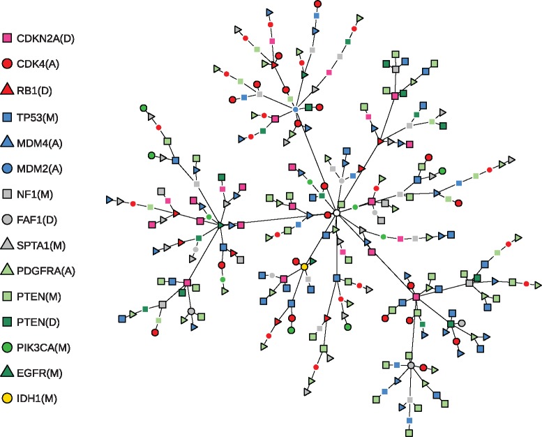
Most likely chronological order of events for all 261 tumours in the glioblastoma dataset. Each of the 193 distinct tumour states corresponds to a terminal node in the tree or an internal node with a black outline and contains all events indicated by the symbols along the trajectory from the starting state (white circle in the centre). The order of events and the unobserved intermediate tumour states (internal nodes without a black outline) were imputed from the estimated transition rate matrix $Q_{\widehat{\Theta }}$. To this end we used the uniformization method (Grassmann, 1977) to construct the time-discretized transition probability matrix $(I+Q_{\widehat{\Theta }}/\gamma )$, where γ is the greatest absolute diagonal entry of $Q_{\widehat{\Theta }}$. The most likely trajectories from the starting state to each observed tumour state were then computed using a single-source shortest path algorithm, where each transition was weighted by the negated logarithm of its probability

The PI(3)K pathway (green) regulates cell proliferation and involves the genes PTEN, PIK3CA, EGFR, PDGFRA. While IDH1 is not a canonical member of the PI(3)K pathway, MHN reports an inhibition between IDH1(M) and PTEN(M) and pathTiMEx groups IDH1(M) together with PTEN(M), PTEN(D) and PIK3CA(M). Notably, MHN inferred that the rare event IDH1(M) promotes the more common event TP53(M). This is further illustrated in Figure 6 which shows the most likely chronological order of events for all 261 tumours. Each of their 193 distinct states is represented by a path that starts at the root node and terminates at either a leaf node or an internal node with a black outline. As can be seen in the lower left, all tumours that contain IDH1(M) are located on a common branch and thus share an early mutation history initiated by IDH1(M). This interpretation is in line with the fact that IDH1(M) is considered a defining attribute of the Proneural subtype of gliobastoma which is clinically distinct and also associated with TP53(M) (Verhaak et al., 2010). It is further supported by independent data from consecutive biopsies of gliomas where IDH1(M) in fact preceded TP53(M) (Watanabe et al., 2009).

4 Discussion

We presented Mutual Hazard Networks, a new framework for modelling tumour progression from cross-sectional observations. MHN are an extension of Conjunctive Bayesian Networks (Beerenwinkel et al., 2007): The multiplicative dependencies between rates [Equation (2)] approximate the conjunctive dependencies of CBNs in the limit of a vanishing baseline hazard (see Supplementary Section S1). MHN are also an extension of Network Aberration Models (Hjelm et al., 2006): NAM also use multiplicative dependencies of rates but restrict hazard ratios to be greater than one, which cannot generate patterns of mutual exclusivity. Moreover, MHN further develop the idea of Raphael and Vandin (2015) and Cristea et al. (2017) that grouping events into ‘pathways’ of mutual exclusive events cannot be done independently from dependencies between pathways. In fact, MHN give up the concept of grouping events entirely. It is not needed anymore, because patterns of mutually exclusive events can be naturally formed by pairwise bidirectional inhibitions or longer inhibiting cycles [such as between TP53(M), MDM2(A) and CDKN2A(D)], both allowing for overlapping pathways. Such overlap exists. The screening approach of Leiserson et al. (2015) finds overlapping gene sets forming patterns of mutual exclusivity, nicely reflecting the fact that several cancer genes participate in multiple pathways (McLendon et al., 2008). However, this approach does not yet embed overlapping pathways into progression models while MHNs do just this.

Still, MHN shares some limitations with earlier models. Kuipers et al. (2017) have shown that back mutations, which MHNs cannot account for, do occur in tumour progression, although not frequently. Our proposed implementation of the MHN learning algorithm has a space and time complexity that is exponential in the number of events n, which compares similarly to Hjelm et al. (2006) and trails (Montazeri et al., 2016). Therefore events have to be pre-selected by recurrency or more sophisticated approaches (Hainke et al., 2017). In practice, we saw limits at n = 25 on a standard workstation. Modern cancer datasets report hundreds of recurrent mutations, and the question arises whether MHN can deal with them. In fact we believe that MHN is competitive with other algorithms also for these large datasets, because interactions between low-frequency events cannot be resolved reliably at all. For example, in the glioblastoma dataset, the rare events OBSCN(M), CNTNAP2(M), LRP2(M), TP53(D) and PAOX(M) remained unconnected to the rest of the network. In other words, the evidence for possible interactions was so low that it could not compensate for the L1-costs of an additional edge. These are limitations in the data itself and not in computation times.

An interesting feature of MHN are the spontaneous occurrence/fixation rates Θ_ii. The event pair IDH1(M) and TP53(M) was instructive for understanding their role. IDH1 mutations were infrequent in the glioblastomas compared to TP53 mutations. Moreover, 10 out of 14 IDH1(M) positive glioblastoma also showed a TP53 mutation. We see at least two alternative explanations for this noisy subset pattern: (1) TP53 mutations are needed for IDH1 mutations to occur. (2) TP53(M) has a much higher spontaneous rate than IDH1(M) explaining that it is more frequent, and moreover, an IDH1 mutation strongly increases the rate of a TP53 mutation, explaining why so many IDH1(M) positive glioblastoma were also positive for TP53(M). While both scenarios explain the noisy subset pattern, they disagree with respect to the chronological order of events. In (1) the TP53 mutation precedes the IDH1 mutation, while in (2) the events occur in reverse order. MHN decided for explanation (2) and is endorsed by independent data from consecutive biopsies (Watanabe et al., 2009). Where in the training data was the evidence in favour of (2) over (1)? If TP53(M) were necessary for IDH1(M), we would expect IDH1(M) to have a very small spontaneous rate in the absence of TP53(M) and hence to occur later than other events, if at all. Yet, of the four cases that were IDH1(M) positive and TP53(M) negative, all of them had at most one mutation in addition to IDH1(M) (Fig. 5A, purple), which is in line with (2) but not with (1).

In summary, we introduced a new, very flexible framework for tumour progression modelling that naturally accounts for cyclic interactions between events.

References

- Akaike H. (1974) A new look at the statistical model identification. IEEE Trans. Automatic Control, 19, 716–723. [Google Scholar]
- Amoia V. et al. (1981) Computer-oriented formulation of transition-rate matrices via Kronecker Algebra. IEEE Trans. Reliabil., R-30, 123–132. [Google Scholar]
- Andrew G., Gao J. (2007) Scalable Training of L1-regularized Log-linear Models. In: Proceedings of the 24th International Conference on Machine Learning, ICML ’07. ACM, New York, NY, USA, pp. 33–40.
- Baudis M., Cleary M.L. (2001) Progenetix.net: an online repository for molecular cytogenetic aberration data. Bioinformatics, 17, 1228–1229. [DOI] [PubMed] [Google Scholar]
- Beerenwinkel N. et al. (2005) Learning multiple evolutionary pathways from cross-sectional data. J. Comput. Biol., 12, 584–598. [DOI] [PubMed] [Google Scholar]
- Beerenwinkel N. et al. (2007) Conjunctive Bayesian networks. Bernoulli, 13, 893–909. [Google Scholar]
- Beerenwinkel N. et al. (2015) Cancer evolution: mathematical models and computational inference. Syst. Biol., 64, e1–e25. [DOI] [PMC free article] [PubMed] [Google Scholar]
- Buchholz P. (1999) Structured analysis approaches for large Markov chains. Appl. Numer. Math., 31, 375–404. [Google Scholar]
- Buis P.E., Dyksen W.R. (1996) Efficient vector and parallel manipulation of tensor products. ACM Trans. Math. Softw., 22, 18–23. [Google Scholar]
- Cerami E. et al. (2012) The cBio cancer genomics portal: an open platform for exploring multidimensional cancer genomics data. Cancer Discov., 2, 401–404. [DOI] [PMC free article] [PubMed] [Google Scholar]
- Ciriello G. et al. (2012) Mutual exclusivity analysis identifies oncogenic network modules. Genome Res., 22, 398–406. [DOI] [PMC free article] [PubMed] [Google Scholar]
- Constantinescu S. et al. (2016) TiMEx: a waiting time model for mutually exclusive cancer alterations. Bioinformatics, 32, 968–975. [DOI] [PubMed] [Google Scholar]
- Cox D.R. (1972) Regression models and life-tables. J. R. Stat. Soc. Ser. B (Methodological), 34, 187–220. [Google Scholar]
- Cristea S. et al. (2017) pathTiMEx: joint inference of mutually exclusive cancer pathways and their progression dynamics. J. Comput. Biol., 24, 603–615. [DOI] [PubMed] [Google Scholar]
- Desper R. et al. (1999) Inferring tree models for oncogenesis from comparative genome hybridization data. J. Comput. Biol., 6, 37–51. [DOI] [PubMed] [Google Scholar]
- Farahani H.S., Lagergren J. (2013) Learning oncogenetic networks by reducing to mixed integer linear programming. PLoS One, 8, e65773.. [DOI] [PMC free article] [PubMed] [Google Scholar]
- Fearon E.R., Vogelstein B. (1990) A genetic model for colorectal tumorigenesis. Cell, 61, 759–767. [DOI] [PubMed] [Google Scholar]
- Gerstung M. et al. (2009) Quantifying cancer progression with conjunctive Bayesian networks. Bioinformatics, 25, 2809–2815. [DOI] [PMC free article] [PubMed] [Google Scholar]
- Gerstung M. et al. (2011) The temporal order of genetic and pathway alterations in tumorigenesis. PLoS One, 6, e27136.. [DOI] [PMC free article] [PubMed] [Google Scholar]
- Grassmann W. (1977) Transient solutions in Markovian queueing systems. Comput. Operat. Res., 4, 47–53. [Google Scholar]
- Hainke K. et al. (2012) Cumulative disease progression models for cross-sectional data: a review and comparison. Biometrical J., 54, 617–640. [DOI] [PubMed] [Google Scholar]
- Hainke K. et al. (2017) Variable selection for disease progression models: methods for oncogenetic trees and application to cancer and HIV. BMC Bioinformatics, 18, 358. [DOI] [PMC free article] [PubMed] [Google Scholar]
- Hjelm M. et al. (2006) New probabilistic network models and algorithms for oncogenesis. J. Comput. Biol., 13, 853–865. [DOI] [PubMed] [Google Scholar]
- Kim Y.-A. et al. (2015) MEMCover: integrated analysis of mutual exclusivity and functional network reveals dysregulated pathways across multiple cancer types. Bioinformatics, 31, i284–i292. [DOI] [PMC free article] [PubMed] [Google Scholar]
- Kuipers J. et al. (2017) Single-cell sequencing data reveal widespread recurrence and loss of mutational hits in the life histories of tumors. Genome Res., 27, 1885–1894. [DOI] [PMC free article] [PubMed] [Google Scholar]
- Leiserson M. et al. (2013) Simultaneous identification of multiple driver pathways in cancer. PLoS Comput. Biol., 9, e1003054.. [DOI] [PMC free article] [PubMed] [Google Scholar]
- Leiserson M. et al. (2015) CoMEt: a statistical approach to identify combinations of mutually exclusive alterations in cancer. Genome Biol., 16, 160.. [DOI] [PMC free article] [PubMed] [Google Scholar]
- McLendon R. et al. (2008) Comprehensive genomic characterization defines human glioblastoma genes and core pathways. Nature, 455, 1061–1068. [DOI] [PMC free article] [PubMed] [Google Scholar]
- Miller C.A. et al. (2011) Discovering functional modules by identifying recurrent and mutually exclusive mutational patterns in tumors. BMC Med. Genomics, 4, 1–34. [DOI] [PMC free article] [PubMed] [Google Scholar]
- Misra N. et al. (2014) Inferring the paths of somatic evolution in cancer. Bioinformatics, 30, 2456–2463. [DOI] [PubMed] [Google Scholar]
- Montazeri H. et al. (2016) Large-scale inference of conjunctive Bayesian networks. Bioinformatics, 32, i727–i735. [DOI] [PubMed] [Google Scholar]
- Nowell P.C. (1976) The clonal evolution of tumor cell populations. Science, 194, 23–28. [DOI] [PubMed] [Google Scholar]
- Ramazzotti D. et al. (2015) CAPRI: efficient inference of cancer progression models from cross-sectional data. Bioinformatics, 31, 3016–3026. [DOI] [PubMed] [Google Scholar]
- Raphael B.J., Vandin F. (2015) Simultaneous inference of cancer pathways and tumor progression from cross-sectional mutation data. J. Comput. Biol., 22, 510–527. [DOI] [PMC free article] [PubMed] [Google Scholar]
- Schwartz R., Schäffer A.A. (2017) The evolution of tumour phylogenetics: principles and practice. Nat. Rev. Genet., 18, 213–229. [DOI] [PMC free article] [PubMed] [Google Scholar]
- Szczurek E., Beerenwinkel N. (2014) Modeling mutual exclusivity of cancer mutations. PLoS Comput. Biol., 10, e1003503.. [DOI] [PMC free article] [PubMed] [Google Scholar]
- Toledo F., Wahl G.M. (2007) MDM2 and MDM4: p53 regulators as targets in anticancer therapy. Int. J. Biochem. Cell Biol., 39, 1476–1482. [DOI] [PMC free article] [PubMed] [Google Scholar]
- Vandin F. (2017) Computational methods for characterizing cancer mutational heterogeneity. Front. Genet., 8, 83. [DOI] [PMC free article] [PubMed] [Google Scholar]
- Verhaak R.G. et al. (2010) Integrated genomic analysis identifies clinically relevant subtypes of glioblastoma characterized by abnormalities in PDGFRA, IDH1, EGFR, and NF1. Cancer Cell, 17, 98–110. [DOI] [PMC free article] [PubMed] [Google Scholar]
- Watanabe T. et al. (2009) IDH1 mutations are early events in the development of astrocytomas and oligodendrogliomas. Am. J. Pathol., 174, 1149–1153. [DOI] [PMC free article] [PubMed] [Google Scholar]
- Yeang C.-H. et al. (2008) Combinatorial patterns of somatic gene mutations in cancer. FASEB J., 22, 2605–2622. [DOI] [PubMed] [Google Scholar]
Associated Data
This section collects any data citations, data availability statements, or supplementary materials included in this article.