Qualifying antibodies for image-based immune profiling and multiplexed tissue imaging

Abstract

Multiplexed tissue imaging enables precise, spatially resolved enumeration and characterization of cell types and states in human resection specimens. A growing number of methods applicable to formalin-fixed, paraffin-embedded (FFPE) tissue sections have been described, the majority of which rely on antibodies for antigen detection and mapping. This protocol provides step-by-step procedures for confirming the selectivity and specificity of antibodies used in fluorescence-based tissue imaging and for the construction and validation of antibody panels. Although the protocol is implemented using tissue-based cyclic immunofluorescence (t-CyCIF) as an imaging platform, these antibody-testing methods are broadly applicable. We demonstrate assembly of a 16-antibody panel for enumerating and localizing T cells and B cells, macrophages, and cells expressing immune checkpoint regulators. The protocol is accessible to individuals with experience in microscopy and immunofluorescence; some experience in computation is required for data analysis. A typical 30-antibody dataset for 20 FFPE slides can be generated within 2 weeks.

Reporting Summary

Further information on research design is available in the Nature Research Reporting Summary.

Introduction

Tissue biopsies and resection specimens are among the most widely acquired patient samples in medicine, and their analysis by anatomic pathologists is the basis for differential diagnosis of many diseases and virtually all cases of cancer. Tissue imaging also plays an important role in many basic and translational studies in developmental biology, pathophysiology, and drug development. In clinical practice, tissue samples are usually FFPE, sectioned, and then stained with H&E following procedures that have been in place for nearly a century. In a subset of cases, molecular diagnosis of such samples is facilitated by immunohistochemistry (IHC), and in a yet smaller number of cases, by RNA and DNA fluorescence in situ hybridization (FISH). IHC of FFPE tissue typically provides data on the level of expression and spatial distribution of a single marker¹, although ‘cocktails’ of two- or three-marker IHC are occasionally used clinically².

The recent development of highly multiplexed imaging technologies raises the possibility of much deeper molecular analysis of human resection specimens and tissues from animal models. Methods that can be implemented on top of universal FFPE-based pathology workflows are particularly promising. In contrast to single-cell sequencing or flow cytometry of disaggregated tissues, highly multiplexed digital histology provides data on cell identity and morphology within a preserved tissue context. Highly multiplexed tissue imaging has many potential applications in basic and translational research and is likely to find wide application in the analysis of clinical trial specimens, where tissue-sparing methods are highly valued, as well as in the clinical workflows used for diagnostic surgical pathology^3–5.

Multiplexed tissue imaging approaches

Some multiplexed tissue imaging methods involve optical imaging, whereas others use ablation—for example, with laser or ion beams—followed by spectroscopy⁴. Ablation methods include multiplexed ion beam imaging (MIBI) and imaging mass cytometry (IMC); these methods achieve a high degree of multiplexing using antibodies as reagents, metals as labels, and mass spectrometry as a detection modality^6–8. Ablation can also be accomplished mechanically. For example, multiplexed spatial assessment of protein expression using NanoString digital spatial profiling relies on optical imaging to guide selection of regions of interest (ROIs), followed by aspiration using a microcapillary and detection of unique oligonucleotide barcodes conjugated to primary antibodies via UV-cleavable linkers⁹. Purely optical methods include multispectral imaging via IHC and sequential chromogenic IHC, and detection of upward of a dozen antigens is possible with these techniques^10–13. Methods such as co-detection by indexing (CODEX)¹⁴, DNA exchange imaging (DEI)¹⁵, MultiOmyx (MxIF)¹⁶, imaging cycler microscopy (ICM)^17–19, and t-CyCIF²⁰, among several others²¹, use fluorescence imaging and various primary/secondary detection chemistries to quantify antigen binding by antibodies. Multiplexed IHC and immunofluorescence (MxIF, t-CyCIF) are potentially the easiest to implement in that they use either conventional primary and secondary antibodies or fluorophore/enzyme-conjugated primary antibodies. Such antibodies are available from many vendors.

The resolution, sensitivity, dynamic range, maximum number of channels, speed, complexity, and cost of tissue imaging methods vary. No comprehensive comparison has been reported, although the features of serial immunofluorescence microscopy and IMC and MIBI have been compared⁴. Images obtained using multiplexed tissue immunofluorescence have the resolution expected of the microscope with which they were acquired. For example, t-CyCIF can achieve super-resolution (<200 nm laterally) with clinical FFPE specimens when performed using structured-illumination microscopy (SIM)²⁰.

Multiple approaches have also been developed for spatially resolved, highly multiplexed imaging of RNA, including spatial transcriptomics²², fluorescent in situ sequencing^23,24, padlock probes and in situ target-primed rolling-circle amplification²⁵, and multiplexed error-robust FISH (MERFISH)^26,27. Analyses of RNA in clinical samples can potentially draw on an immense and rapidly growing body of genomic and molecular data but can also be problematic to perform because of the lability of RNA and the complexities of standardizing pre-analytical variables in many clinical settings^28,29.

Regardless of how antibody–antigen conjugates are detected, virtually all multiplexed tissue imaging techniques (e.g., MIBI, IMC, MxIF, CODEX, ICM, DEI, and t-CyCIF) involve the use of primary antibodies. Extensive literature exists on immunostaining in research and clinical settings, and it is well established that specificity and reproducibility are influenced by a range of analytical factors that include dilution, incubation conditions, type, context in which the antibody was generated (e.g., tissue-based work or flow cytometry), and the extent of conjugation³⁰. Some commercially available antibodies work well, whereas others work poorly or not at all. Ongoing assessment is also necessary to reaffirm the reliability of antibodies that do work by actively monitoring staining across tissue types and batches of reagent.

Overview of the procedure

In this protocol, we describe how to construct and validate antibody panels for immune profiling of human tumors using t-CyCIF. The procedure covers methods for immune panel assembly and validation that include slide staining and image acquisition (Steps 1–31), image processing (Steps 32–34), and multiple techniques for data visualization (Steps 35–41). These methods can be implemented by most laboratories familiar with immunofluorescence using a variety of microscopes, although each lab should take care to implement appropriate calibration protocols and controls. We describe the development of a 16-marker panel for characterizing canonical immune cell types, as well as cell proliferation with Ki-67 staining and cell lineage with glial fibrillary acidic protein (GFAP), an intermediate filament protein, alpha-smooth-muscle actin (α-SMA), and a pan-isoform keratin epitope. We discuss factors that impact the assembly of panels and present example data for a 16-plex panel that uses binary gating to enumerate canonical immune cell types (B cells, helper and cytotoxic T cells, regulatory T (T_reg) cells, natural killer (NK) cells, macrophages, and dendritic cells) with the potential to differentiate into 65,000 states (Supplementary Fig. 1).

We envision that successful immune cell profiling will require the ability to innovate quickly in the context of the torrent of new data on immuno-oncology as well as a commitment to the free and open sharing of information, reagents, methods, and computational tools, some of which will be reduced to practice by industry for general clinical use. Our group is developing an antibody validation resource at https://www.cycif.org/ comprising a list of reagents, images, caveats, and best practices. The site also describes data analysis, visualization, and management software needed to construct pre-cancer and cancer atlases³¹. We are also performing cross-platform comparison to assist laboratories using MIBI, CODEX, or DEI. We hope that instrument and antibody suppliers will respond to these academic efforts by manufacturing quality-controlled panels for clinical use.

Using t-CyCIF for antibody validation

For this protocol, we use t-CyCIF²⁰, an extension of older approaches to the sequential assembly of multiplex images using fluorophore inactivation and/or antibody stripping. However, this validation approach is applicable to many other imaging methods, and we anticipate that primary antibodies successfully tested with t-CyCIF can also be used in other tissue imaging approaches. t-CyCIF constructs high-dimensional images via sequential four- to six-color immunofluorescence imaging on a conventional microscope and can be extended to at least 60 antigens. In general, we find that the fluorophore inactivation process, which is based on light- and acid- or base-catalyzed oxidation, substantially reduces autofluorescence, and that the signal-to-noise ratio can therefore increase with cycle number. For many antibodies, the order of addition does not appear to be critical, and preservation of immunogenicity and morphology is excellent across many staining cycles. However, there is a subset (~15–20%) of antibodies that increase in intensity with cycle number and a similar fraction of antibodies that decrease in intensity. It is important to test and control for such effects (see ‘Considerations in the construction of antibody panels’ section)^16,17,20. To date, we have tested primary antibodies against cell cycle regulators, signaling proteins and kinases, cell lineage markers, transcription factors, multiple cell state markers²⁰, and a wide range of immune markers (see https://www.cycif.org/ for details)^20,32,33. Efforts are also underway to integrate multiplex immunofluorescence imaging with FISH, in situ mRNA profiling, and DNA mutation detection^16,34–38 as part of a multi-parametric approach to tumor characterization and human tumor atlas construction.

One advantage of methods such as t-CyCIF is that individual investigators can create and test their own antibody panels using readily available microscopes and standard reagents in a mix-and-match approach that is adaptable to specific tissue types and scientific questions. It seems very likely that antibodies well-suited to t-CyCIF will largely be compatible with IMC, MIBI, DEI, CODEX, and multiplexed IHC methods as well, because the method of antigen detection is fundamentally similar. The primary difference among these approaches involves the mode of detection (i.e., the atoms or molecules conjugated to the primary antibody). Antibody panels should also be similar across these methods, perhaps with small modifications such as differing dilutions. Data visualization and analysis are also very similar for t-CyCIF²⁰, MxIF¹⁶, multiplexed IHC², and MIBI⁸. Nonetheless, platform-specific confirmation of the performance of antibodies and algorithms may be required because labeling with dyes and metals may result in different sensitivities and specificities, as well as different levels of background and dynamic range.

Applications of the approach

Recent interest in multiplexed histology in cancer is driven in part by the introduction of immune checkpoint inhibitors (ICIs), which are expanding treatment options for many solid and hemato-logical malignancies^39–41. ICIs disrupt cell-to-cell interactions in a non-cell-autonomous manner and activate normal tumor surveillance by the immune system. Knowing the numbers, types, and locations of immune cells in the tumor microenvironment is thought to be essential to understanding mechanisms of action^39,42,43. The use of ICIs as first-line therapeutic agents^44,45 and as neo-adjuvant therapies⁴⁶ is increasingly common. Specifically, targeting the immune checkpoints mediated by cytotoxic T lymphocyte-associated antigen-4 (CTLA-4), programmed cell death-1 receptor (PD-1), and programmed cell death ligand 1 (PD-L1) has been shown to elicit marked therapeutic responses in a range of cancers, including advanced non-small-cell lung carcinoma, melanoma, renal cell carcinoma, and Hodgkin lymphoma^47–53.

Even in the case of tumor types that are broadly ICI-responsive (e.g., melanoma), not all patients benefit from existing drugs, and there are many types of tumors (e.g., triple-negative breast cancer) in which only sporadic responses are observed. Thus, predictive biomarkers are needed. These biomarkers are likely to require the use of multiplex panels that enable ‘immune profiling’ to determine the abundance, locations, and states of tumor-associated immune cells and the levels of expression of ICI ligands and receptors on immune and tumor cells^39,42,43,54. Relevant intracellular states for immune cells include degree of activation and exhaustion⁵⁵, rate of proliferation, degree of apoptotic priming, and levels of replication, metabolic, and other stresses^56,57.

Multiplex flow cytometry suggests that 12–14 cell surface markers can provide a basic enumeration of T- and B-cell subtypes, although the number will vary depending on the research question or pathologic diagnosis being addressed. Identifying stromal and tumor cells and their states is likely to require a similar number of markers. In addition, multiple checkpoints are currently being targeted therapeutically: approved drugs exist against PD-1, PD-L1 and CTLA-4, and multiple phase II/III trials are ongoing for drugs targeting lymphocyte-activation gene 3 (LAG3), T-cell immunoglobulin mucin-3 (TIM3), and T-cell immunoreceptor with Ig and ITIM domains (TIGIT)^58,59. Biomarker discovery for ICIs will require the ability to rigorously enumerate cell types and states on the basis of their levels of expression of 20–40 immunofluorescence markers^60–64. Ideally, these measurements can be made using technical platforms that allow individual research teams to develop and test new ‘mix-and-match’ assays for specific drug targets, immune cell populations, and tumor biomarkers.

Future directions

In the future, we anticipate that human and mouse tissues will be studied using protein imaging, dissociated single-cell RNA-seq, spatial transcriptomics, and multiparameter flow cytometry and mass cytometry (CyTOF) in parallel^65–67. Multi-modal approaches such as these could provide unprecedented insights into cellular phenotypes and disease processes. We also expect improvements in throughput; in the case of t-CyCIF, this will involve increasing the number of channels imaged in each cycle so that fewer cycles are needed to construct deep profiles, as well as improvements in all the downstream data collection and analysis steps.

Expertise needed to implement the protocol

The methods described below are accessible to research assistants, graduate students, and post-doctoral fellows with experience in microscopy and immunofluorescence. Specialized experience in tissue imaging and histopathology is not required, but some experience with computational tools is needed to analyze the data. Implementing these approaches on other platforms (e.g., MIBI, IMC, DEI, or CODEX) depends largely on the availability of labeled antibodies and proprietary reagents; users of these methods should contact the relevant manufacturers.

Experimental design

Imaging on a slide-scanning microscope

A variety of fluorescence microscopes can be used to image slides, but good stage control and stable illumination are essential for generating high-quality and comparable data. Methods for calibrating fluorescence microscopes for use in quantitative studies are described in detail elsewhere^68,69. We have tested a Leica Aperio Digital Pathology Slide Scanner, a GE IN-Cell Analyzer 6000, a GE OMX-SR Super-Resolution Microscope, and a GE Cytell Cell Imaging System. Hamamatsu, Nikon and other companies also manufacture suitable instruments. The principal requirements for these instruments are as follows:

• The ability to acquire at least four-channel images without spectral interference,

• A stage that grasps slides firmly and consistently, and

• The ability to store and retrieve exact slide positions between cycles.

The speed, resolution, signal-to-noise ratio, and number of available fluorescence channels will vary with the microscope. We routinely perform immune profiling using wide-field microscopes with air objectives having numerical apertures (NAs) of ~0.2–0.6, but higher-resolution instruments, such as confocal, deconvolution, and structured-illumination microscopes, make it possible to capture fine subcellular detail. The GE IN Cell Analyzer 6000, GE OMX-SR, and RareCyte CyteFinder HT are among our instruments of choice (Table 1). In this study, we used the RareCyte CyteFinder, which is capable of six-channel, whole-slide imaging and precise slide positioning (note that only four channels were used for the work described here). We use Imager 5 software (RareCyte) for data acquisition.

Table 1 |.

Features of microscopes used in this study and our prior studies

Instrument	Type	Objective	Field of view (mm)	Nominal resolution (μm)a
RareCyte CyteFinder	Slide scanner	10×/0.3 NA	1.6 × 1.4	1.06
		20×/0.8 NA	0.8 × 0.7	0.40
		40×/0.6 NA	0.42 × 0.35	0.53
GE IN Cell Analyzer 6000	Slide scanner	10×/0.45 NA	1.3 × 1.3	0.70
		20×/0.75 NA	0.66 × 0.66	0.42
		40×/0.95 NA	0.33 × 0.33	0.33
		60×/0.95 NA	0.22 × 0.22	0.33
GE IN Cell Analyzer 6000	Confocal	60×/0.95 NA	0.22 × 0.22	0.21
GE OMX Blaze	SIM	60×/1.42 NA	0.08 × 0.08	0.11

^aExcept for the OMX Blaze, we calculated the nominal resolution (r) with the formula: r = 0.61λ/NA for widefield or r = 0.4λ/NA for confocal microscopy (λ = 520 nm). The actual resolution depends on optical properties, the thickness of the tissue section, and both the alignment and the quality of the optical components used. For SIM, the actual resolution depends on accurate matching of the immersion oil refractive index with the particular sample in the Cy3 channel and the use of an optimal point spread function during the reconstruction process. The resolution in other channels will be lower.

Tissues and cells for antibody testing (controls)

Selecting an appropriate set of samples for any tissue imaging project is obviously of paramount importance, but it is beyond the scope of the current article; a discussion of factors affecting study design and statistical analyses can be found elsewhere^70–72. In general, a range of sample types is used for antibody validation, including clinical specimens with known genetic alterations. For example, one can use malignant peripheral nerve sheath tumors with EED or SUZ12 mutations for testing antibodies against H3K27me3, or mismatch repair–deficient tumors carrying inactivating alterations for testing antibodies against MSH2/MSH6 or MLH1/PMS2. In both instances, there is a highly characteristic loss of signal in tumor cells, with retention of signal in non-neoplastic (and genetically wild-type) stromal cells and neighboring normal tissues. Other FFPE tissue samples useful for antibody validation include specimens with known patterns of protein expression (e.g., certain hormone receptors in breast or prostate cancer) or tissues containing cells from defined lineages (e.g., kidney/upper urinary tract and the Müllerian system for validating PAX8 antibodies, skin for MITF antibodies, brain for OLIG2 antibodies, breast for GATA3 antibodies, and prostate for NKX3.1)⁷³. Such FFPE validation samples can be compiled into tissue microarrays (TMAs) that allow investigators to not only assess the sensitivity but also the specificity of the antibody reagents across dozens of normal and pathologic tissue types.

Other reagents commonly used for antibody validation include cell lines that have been subjected to small interfering or short hairpin RNA(si/shRNA) knockdown, CRISPR–Cas9 genome editing⁷⁴, open-reading-frame overexpression, drug or chemical exposure, or environmental manipulation⁷⁵. Cultures of these cell lines are pelleted, fixed, and embedded in FFPE blocks in the same manner as tissues. Blocks with individual cell lines are then assembled into cell line microarrays (Box 1). Antibody validation can also be performed following conventional protocols for staining cultured cells or following cell-based CyCIF⁷⁶, but this approach is less ideal because of the impact of different fixation conditions on antibody performance.

Box 1 |. Creating FFPE cell line microarrays for antibody testing ● Timing 17 h.

Procedure

! CAUTION Follow local biosafety guidelines for details on handling of biohazardous materials.

1. Assemble a suitable panel of genetically engineered or drug-treated cell lines.

2. Heat HistoGel to 60 °C to liquefy the solution.

3. Collect cells from confluent T75 flasks or 10-cm dishes (~5 million cells) into a 15-ml Falcon tube.

4. Centrifuge the samples at 200g for 5 min at RT.

5. Remove the supernatant.

6. Resuspend cell pellet in 500 μl of 4% (wt/vol) phosphate-buffered formaldehyde or 10% (wt/vol) phosphate-buffered formalin and fix at 4 °C for 15 min.

   ▲CRITICAL STEP Do not overfix the samples; this can affect antigen-antibody binding.

7. Centrifuge samples at 200g for 5 min at RT.

8. Remove the supernatant.

9. Resuspend cell pellet with 1 ml of PBS to wash.

10. Centrifuge the samples at 200g for 5 min at RT.

11. Remove the PBS.

12. Cut off the distal end (1 cm) of a 1-ml pipette tip and gently resuspend the cell pellet in 300 μl of warm HistoGel.

13. Place the HistoGel with cells on a piece of Parafilm to allow a droplet to form.

14. Incubate at 4 °C for 1 h to allow the HistoGel droplet to harden.

15. Subject the HistoGel droplet to standard paraffin embedding to create an FFPE block.

    ▲CRITICAL STEP Do not leave the sample in HistoGel without further processing into paraffin blocks for longer than a couple of days.

    ▲CRITICAL STEP We recommend doing this step at a core facility, which usually has automated instruments to do this in 16 h. In general, the HistoGel droplets are placed into an embedding cassette, dehydrated with two changes of 70% (vol/vol) ethanol for 1 h each, one change of 80% (vol/vol) ethanol for 1 h, one change of 95% (vol/vol) ethanol for 1 h, three changes of 100% ethanol for 1.5 h each, three changes of xylene for 1.5 h each, two changes of paraffin wax for 2 h each at 60 °C, and embedding of the tissue into the paraffin block.

16. Cut 5-μm sections from the FFPE tissue block and mount on slides.

    ■PAUSE POINT Optimal results are obtained using freshly cut FFPE sections mounted on glass slides. Unstained sections can be stored at RT or 4 °C, with the important caveat that a substantial decrease in signal can occur for some antibodies when staining is performed on slides that have been stored for several months, particularly those kept at RT.

When using any tissue or cell line bank for antibody testing, staining should be evaluated for subcellular localization (e.g., nucleus, membrane, endoplasmic reticulum, or cytoplasm), cell type (e.g., tumor or stromal cells), strength of signal, signal-to-noise ratio, and dynamic range (Supplementary Table 1). During antibody validation, we typically initiate testing of fluorophore-conjugated antibodies at a concentration of 10 μg/ml and use a concentration that gives optimal signal strength and signal-to-noise ratio.

Approaches to antibody testing and qualification

There is no single approach to testing antibodies for tissue-based imaging, particularly in the case of human samples. Moreover, no antibody is ever fully ‘validated’, because the pattern and intensity of staining are always subject to unknown confounders arising from pre-analytical variables encountered during sample acquisition and preparation^77,78 and from analytical variables encountered during sample processing and analysis. Instead, a variety of different approaches are needed, depending on the sample and the antibody being studied (Fig. 1). These approaches include (i) comparing patterns of staining by different antibodies on the same sample, which is particularly useful when highly qualified US Food and Drug Administration–approved antibody reagents are available as comparators (e.g., anti PD-1 antibodies⁷⁹); (ii) examining patterns of staining in tissues having stereotypical structures and spatial distributions of multiple cell types (e.g., immune cells in tonsil); and (iii) staining tissues with known genetic lesions such as HER2 overexpression or CDKN2A deletion. This last approach is particularly effective in the case of antibody panels for profiling mouse tissues, and these panels can often be tested using genetically engineered mouse models, although this is beyond the scope of the current protocol. See Box 2 and Figs. 2–4 for a detailed description of how we used these different antibody validation procedures to assemble a 16-antibody immune marker panel.

Fig. 1 |. Schematic of antibody validation approaches for multiplexed tissue imaging.

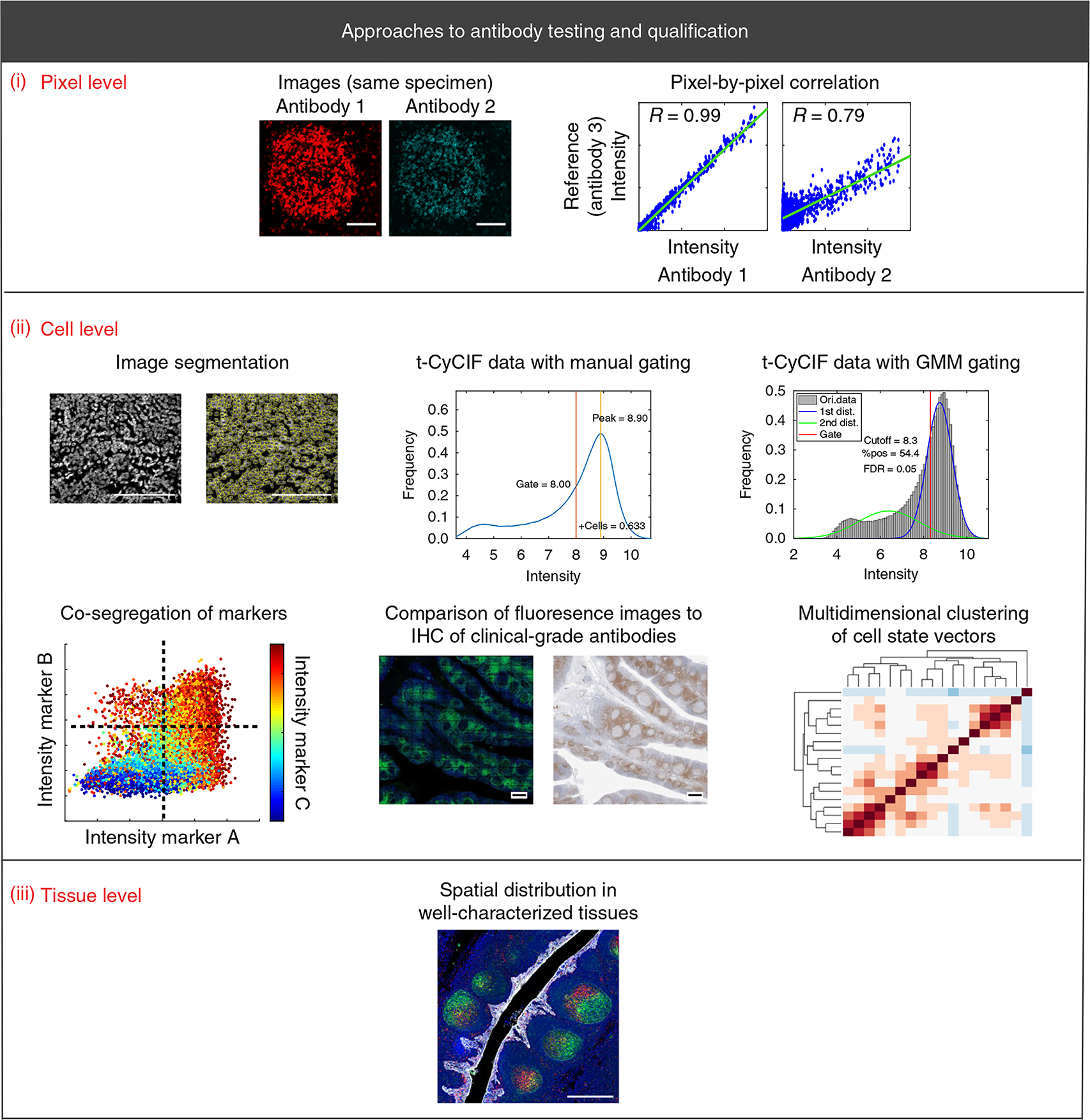
The displayed approaches are the cornerstone methods for validating antibodies for use in any multiplex imaging method. (i–iii) Validation approaches are described at the pixel level (i; scale bars, 100 μm), cell level (ii; scale bars, 100 μm (top left); 500 μm (bottom center)), and tissue level (ii; scale bar, 500 μm). Each approach is discussed in detail in the text. Dist., distribution; FDR, false-discovery rate; Ori., original; pos., positive; R, Pearson correlation coefficient.

Box 2 |. Practical implementation of a 16-antibody immune marker panel.

This box describes how we used different antibody validation procedures to assemble a 16-antibody immune marker panel. To assemble a panel of antibodies for immune profiling, we used normal human tonsil specimens. For immune markers for which multiple antibodies were available, we performed pixel-by-pixel comparison across one or more cycles of t-CyCIF. As noted in the ‘Experimental design’ section, multi-channel fluorescence imaging is greatly superior to IHC in this setting, because antibodies labeled directly or indirectly with different fluorophores can be mixed and used to stain a single tissue section. In other cases, we compared fluorescence and IHC images or used tissue-level data. The large numbers of fluorophore-conjugated antibodies available commercially for many immune markers make all three approaches useful.

Antibody validation by pixel-by-pixel comparisons

A single FFPE section of human tonsil was stained with four different commercially available antibodies against PD-1. This included two chemically conjugated antibodies—PD-1 clone EPR4877(2), which is conjugated to Alexa Fluor 647, and PD-1 clone NAT105, which is conjugated to Alexa Fluor 488—and two unconjugated antibodies, PD-1 clone EH33 (mouse) and PD-1 clone D4W2J (rabbit) (Fig. 2 and Supplementary Tables 1 and 2). For EH33 and D4W2J, detection involved indirect immunofluorescence with Alexa Fluor 647–labeled anti-rabbit for EH33 and Alexa Fluor 555–labeled anti-mouse for D4W2J.

We found that staining from all four antibodies co-localized to the plasma membrane of cells in tonsil germinal centers (Fig. 2), which are lymphoid structures that contain large numbers of follicular T helper cells that are known to express PD-1 (ref.¹¹¹). Pixel-by-pixel comparison of fluorescence intensity values showed that signals from three of the antibodies were highly correlated (Pearson correlation = 0.99), whereas the signal from clone NAT105 had a lower dynamic range and was less well correlated (Pearson correlation = 0.79–0.80; Fig. 2 and Supplementary Table 1). We interpreted the low correlation to be a consequence of both non-selective antigen binding and weaker signal. We selected PD-1 clone EPR4877(2) for the immuno-profiling panel because of its wide dynamic range (14,300 ± 5,800 fluorescence intensity arbitrary units) and the availability of a t-CyCIF-compatible fluorophore-conjugated antibody (see ‘Experimental design’ section).

Pixel-by-pixel comparison was also used to test other antibodies, including three PD-L1 antibodies (Supplementary Fig. 2), two FOXP3 antibodies (Supplementary Fig. 2), three CD45 antibodies (Supplementary Fig. 3), five LAG3 antibodies (Supplementary Fig. 4), and three CD11b antibodies (Supplementary Fig. 5). In each case, antibodies selected for inclusion in the multiplex profiling panel were prioritized on the basis of pixel-by-pixel correlation values with comparators, dynamic range, and the availability of fluorophore-conjugated antibodies (Supplementary Tables 1 and 2). The methods that were used to assess each antibody are listed in Supplementary Table 3.

Antibody validation by comparison to established, clinical-grade IHC antibodies

Sixteen of the most promising antibodies against immune cell markers (as determined from the multiple validation methods shown in Fig. 1 and indicated in Supplementary Table 3) were combined with pan-keratin, GFAP, α-SMA, and Ki-67 antibodies in a 20-antibody panel that was then used for 9-cycle t-CyCIF staining of tonsil tissue (Table 2, Supplementary Table 3). The panel was designed to distinguish immune subtypes, tumor cells, and stromal cells, and to identify proliferating cells of all types.

Patterns of t-CyCIF staining were compared with IHC staining patterns for eight antibodies (CD3, CD4, CD8, CD20, CD68, PD-1, PD-L1, and FOXP3) that are routinely used for clinical diagnosis by the Anatomic Pathology service at Brigham and Women’s Hospital (Fig. 3, Supplementary Table 4, and Supplementary Fig. 6), as well as by clinical services at other medical centers. Such antibodies are the backbone of contemporary immune profiling³⁹. As judged by two trained pathologists, the fluorescence-conjugated and IHC antibodies showed similar patterns of staining. In particular, the expected immune cell subtypes localized to the appropriate tonsil compartments in whole-slide images. For example, small cells positive for CD20 staining were highly enriched in germinal centers, which contain many B cells, whereas CD4⁺ and CD8⁺ cells were found predominantly in tissue surrounding the germinal centers, which contain many T cells (Fig. 3 and Supplementary Fig. 6). Large, irregular CD68⁺ cells were enriched in germinal centers, which contain numerous macrophages that phagocytose B cells undergoing apoptosis. In addition, antibodies against Ki-67, CD19, CD14, CD163, and IBA1 exhibited staining consistent with the established intra-tissue distribution of cycling cells, B cells, and macrophages.

To quantify the fraction of cells positive for IHC staining in tissue sections adjacent to the section used for t-CyCIF, we used standard Aperio ImageScope software. We observed a high degree of correlation between the number of positive cells identified by IHC and the number identified by t-CyCIF for all eight markers for which comparison was possible. For this analysis, a total of ~288,000 cells were successfully segmented in the t-CyCIF data and ~80,000–237,000 cells were segmented from slides subjected to IHC. The Pearson correlation between the number of positive cells determined by IHC and that determined by manual gating of t-CYCIF data across all eight markers was 0.98 (Fig. 3). A strong correlation was also observed when fluorescence intensity distributions were gated using GMMs (Fig. 3; Pearson correlation = 0.95).

Antibody validation by co-segregation of markers across a tissue

Next, we performed tissue-level analysis by asking whether observed patterns of co-staining were consistent with prior knowledge of immune marker expression in specific sub-populations of immune cells found in human tonsil. To look for co-staining, intensity data for each segmented cell were visualized in two-way scatter plots (Fig. 4, Supplementary Figs. 7 and 8, and Supplementary Movie 1). This analysis revealed co-segregation of markers such as PD-1 and CD3, CD8a and CD3, PD-L1 and IBA1, CD3 and CD45RB, and FOXP3 with both CD4 and CD3 (Fig. 4 and Supplementary Fig. 7). Moreover, we found that a subset of T cells co-expressed LAG3 and PD-1, a phenotype that is indicative of T-cell exhaustion. Some cells co-expressed CD163 and IBA, two markers of macrophage lineages. Taken together, pixel-level analysis, comparison of immunofluorescence staining with established IHC patterns, and tissue-level analysis suggested that our profiling panel was selective and reproducible.

Fig. 2 |. Pixel-by-pixel validation of antibodies against PD-1 using t-CyCIF in human tonsil.

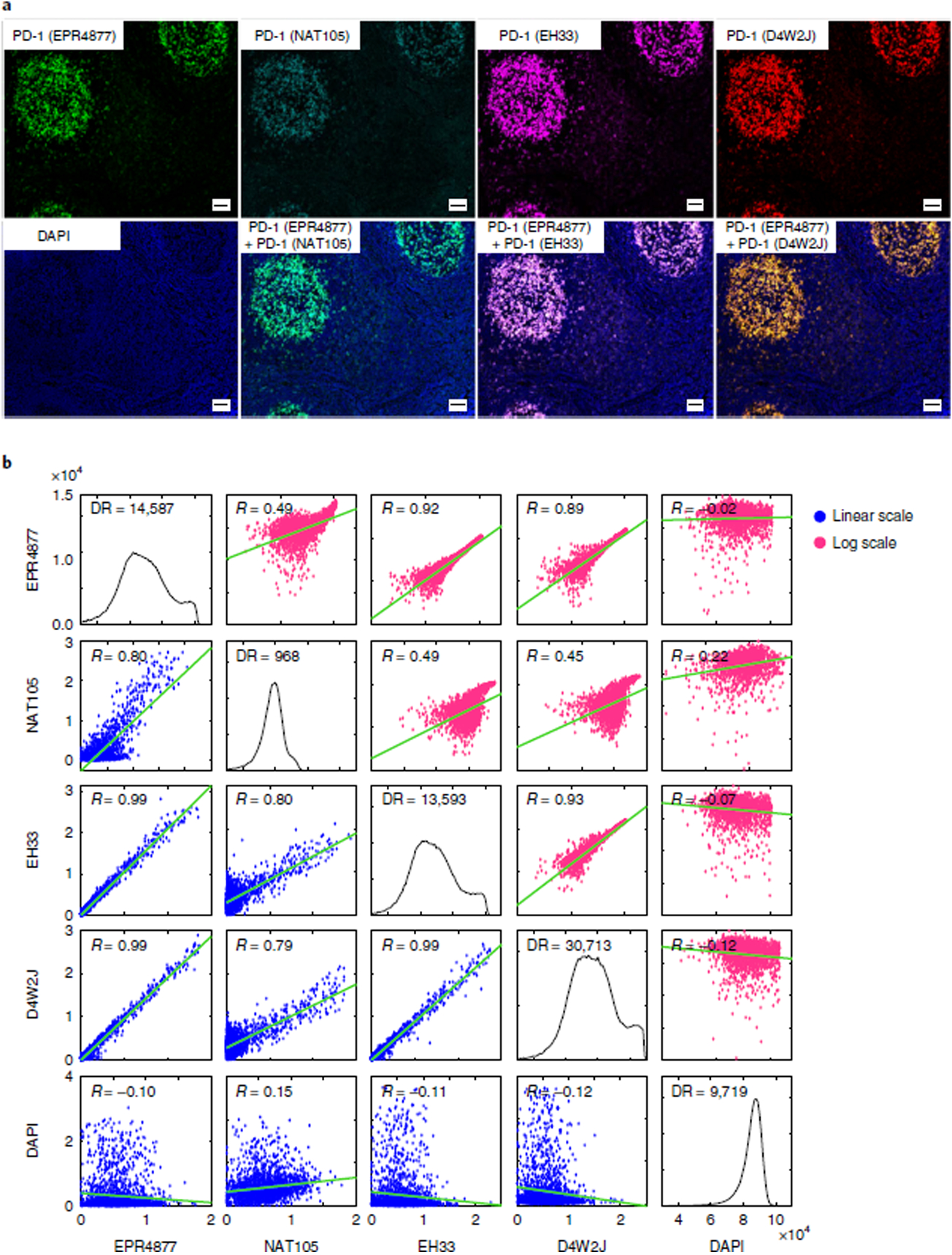
a, Representative images of immunofluorescence staining from human FFPE tonsil sections using four different PD-1 antibodies: EPR4877, Abcam; NAT105, Abcam; EH33, CST; and D4W2J, CST. The DAPI image from the same region, as well as merged images of EPR4877 with NAT106, EH33 and D4W2J, is shown. Scale bars, 50 μm. b, Plots of the pixel-by-pixel correlation of the signal intensity of the four PD-1 antibodies. The plots display the correlation of a random sampling of 2,000 pixels. The plots on the lower left (with blue dots) show the original fluorescence intensity at each pixel, and the plots on the upper right (with magenta dots) show the log-transformed fluorescence intensity at each pixel. Pearson correlation coefficients (R) are shown. The dynamic range and correlation values from five different regions are presented in Supplementary Table 1. DR, dynamic range.

Fig. 4 |. Validation of antibodies for immune profiling by co-segregation of known markers and expected spatial localization.

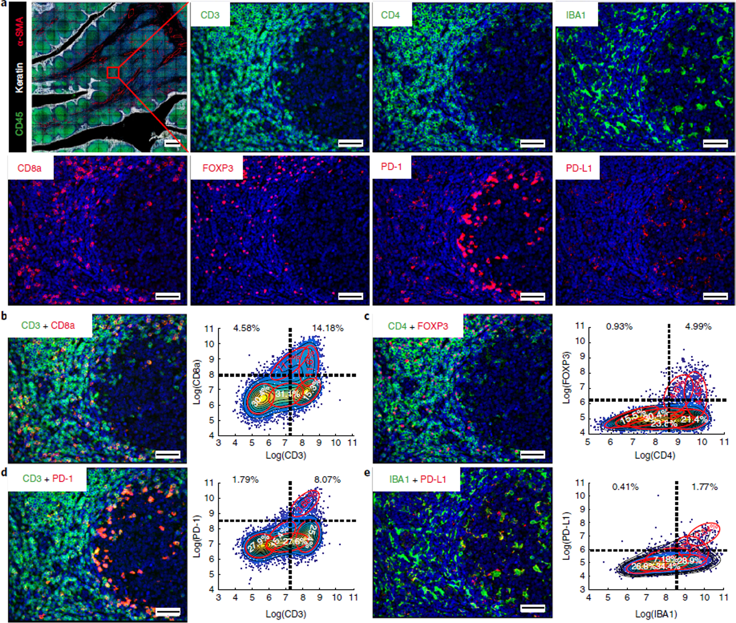
a, Representative images of CD45 (green), keratin (white), α-SMA (red), CD3, CD4, IBA1, CD8a, FOXP3, PD-1, and PD-L1 staining. b–e, (Left) merged images from human tonsil: CD3 + CD8a (b); CD4 + FOXP3 (c); CD3 + PD-1 (d); IBA1 + PD-L1 (e). A compilation of images for all other immune markers is available in Supplementary Movie 1 and Supplementary Figs. 11 and 12. (Right) Corresponding scatter plots were created from a random sampling of data from 10,000 cells. Both manual gating (black dashed lines) and GMM analysis (red ovals) highlight positive and negative cell populations. Scale bars, 500 μm (a, top left), 50 μm (a, all others).

Comparing multiple antibodies

Antibodies can be compared with each other at the level of pixels, cells, or tissues (Fig. 1; see below). In all cases, the starting point is an image in which different cycles of imaging of multiple antibody clones (to both the same and different targets) from the same tissue section have been correctly registered to each other. We have created the open-source ASHLAR algorithm (https://github.com/sorgerlab/ashlar) for joining together (stitching) successive image panels and then registering images across channels. ASHLAR improves on methods currently available in ImageJ (https://imagej.nih.gov/ij/) and is compatible with any image format complying with the Bio-Formats standard^80–83.

• Pixel-level analysis. The signals generated from two or more antibodies that selectively detect the same protein should, in principle, be highly correlated with each other down to the resolution of the microscope. This can be assessed by measuring the correlation between images at the level of individual pixels (Fig. 1, (i)). Image segmentation and morphological analysis are not necessary, and the analysis is therefore straightforward and objective, although accurate registration and correction for chromatic aberration are necessary. Pixel-level Pearson correlation on either a log or linear scale is the preferred method for comparing antibodies against the same antigen when labeling with different fluorophores is possible. This can be achieved by using indirect immunofluorescence and primary antibodies derived from different species, or antibodies chemically conjugated to different fluorophores. Images from different channels are then registered and compared directly. Changing the order of antibody addition may be needed to ensure that differences in signal do not result from saturation of the epitope and steric hindrance.

• Cell-level analysis. When fluorescence images are compared with IHC images and/or two different IHC antibodies are compared with each other, it is almost always necessary to use successive tissue slices. In this scenario, different cells are stained and pixel-level comparison is not meaningful. Instead, cell-level analysis usually involves image segmentation, scoring of positive and negative cells, and then correlating the number of positives and negatives across sections (Fig. 1, (ii)). Matching morphologies and staining patterns across different cells is inherently more subjective than pixel-level analysis and, at the current state of the art, human judgment is often required. However, the introduction of machine-learning methods, which have demonstrated superhuman performance in other medical imaging tasks⁸⁴, may change this. Conventional computer-assisted cell-level analysis involves three sequential steps. First, cell boundaries are identified by computational segmentation, followed by integration of signal intensity across each cell, channel by channel, while subtracting background signal. Second, distributions are constructed for the integrated staining intensity in each channel and analyzed manually or automatically to score positive and negative populations. This yields a high-dimensional cell state vector in which both absolute intensities and correlations between these intensities are informative, e.g., a CD4⁺CD8⁺ double-positive thymocyte is different from a thymocyte positive for either marker alone. Third, correlations among state vectors for different cells are visualized using tools and methods such as multi-axis scatter plots, t-distributed stochastic neighbor embedding (t-SNE) plots, and X-shift plots. These approaches help to cluster cells with similar state vectors and lineage markers. More rigorous, multivariate statistical analyses can then be used to quantify the nature and degree of similarity or difference, for example, by discriminant analysis⁸⁵ or principal component analysis⁸⁶. Spatial analysis can also be performed to determine whether different cell populations (i.e., cells whose state vectors are similar) have a particular spatial relationship to each other. Additional analytical methods include computational analysis of cell and tissue morphology (e.g., to identify membranes, blood vessels, or subcellular organelles and the cytoskeleton). For simplicity, we do not describe these approaches and refer readers to methods for proximity analysis in multiplexed tissue described in the literature^20,87.

• Tissue-level analysis. Tissue-level analysis provides information on the spatial distribution of cells, cell state attributes, membranes, tissue boundaries, and structures such as blood and lymphatic vessels (Fig. 1, (iii)). In computer-assisted tissue-level analysis, the positions (centroids) of individual cells are typically recorded, making it possible to revisit individual cells for further analysis or human inspection. Antibody testing and validation at the level of tissues is most effective using tissues that have a stereotypical distribution of cell types. One of the most frequently used is tonsil; it contains a wide variety of immune cell types compartmentalized in primary lymphoid follicles and secondary lymphoid follicles with germinal centers (e.g., https://www.proteinatlas.org/learn/dictionary/normal/tonsil). Tonsils are also readily available under discarded-tissue protocols, and FFPE specimens can be purchased from commercial vendors including Origene, Pantomics, and GeneTex. Tissue-level analysis of experimental samples typically involves the specification of ROIs, such as tumor and non-neoplastic tissues surrounding the tumor, and calculation of relative levels of staining in different ROIs. For example, the extent of tumor infiltration by immune cells is often highly non-uniform, and immune cells can be substantially more abundant in an ROI corresponding to the tumor/stroma interface than the tumor interior. ROIs can be defined manually by pathologists on the basis of classic morphological criteria following H&E staining. Tumor markers such as pan-keratin (an epitope shared among multiple keratin isoforms) or stromal markers such as α-SMA assist in the identification of ROIs. In this protocol, we use an objective approach to ROI definition based on a K-nearest neighbor (KNN) algorithm. KNN iteratively assesses whether a cell and its neighbors express tumor markers, assigning those that do to the tumor ROI and those that do not to the non-neoplastic tissue.

Cell-type identification

The identification of immune cell types is typically based on an assessment of the presence or absence of expression of cluster of differentiation (CD) proteins and other cell surface markers, as well as lineage-specific transcription factors. The binary antigen-positive or antigen-negative score across multiple markers identifies the cell type; the greater the number of markers, the more precise the subtyping (e.g., CD4⁺CD8⁺ staining identifies double-positive T cells). The assumption is typically made that the presence or absence of CD markers is dependent upon cell type. The multi-channel distribution of staining intensities for a cell therefore represents its identity, convolved by measurement of noise, and intrinsic cell-to-cell variability (Fig. 1). Designating immune cell types from image data in this manner starts with the subtraction of fluorescence signals arising from autofluorescence and nonspecific antibody binding, segmenting the image to identify individual cells, and then integrating staining intensity over each cell.

• Image segmentation. Segmenting images of densely packed cells is a challenging task, particularly when cells of different sizes and shapes are intermingled in tissues⁸⁸. Segmentation is the focus of an entire subfield of machine vision^89,90, and new approaches that learn directly from pixel-level data (bypassing segmentation altogether) are also in development. The approaches described in this protocol represent a good starting point for high-dimensional image analysis, but they are among the simplest available; users may therefore wish to investigate other options. We typically apply standard watershed algorithms in ImageJ or MATLAB (available at our GitHub repository: https://github.com/sorgerlab/cycif) to identify Hoechst 33342–stained nuclei imaged in the ‘DAPI’ channel, and then dilate the nuclear mask to encompass a representative portion of the nucleus. ilastik is also a good alternative (https://www.ilastik.org/). Staining intensity is integrated over the cytoplasm, the nucleus, or both compartments. Making masks slightly larger than a typical lymphocyte (~10 μm in diameter) is generally sufficient to quantify cell surface staining. A rolling-ball algorithm is used to remove global and regional background for each channel²⁰. Evaluation of image segmentation and an assessment of the types of errors that typically occur is shown below in the ‘Anticipated results’ (Supplementary Fig. 9).

• Manual gating to identify cells with positive or negative staining. The intensity distribution obtained after image segmentation can be analyzed manually or automatically to identify positive and negative populations (Fig. 1, (ii); a manual gating example is shown in Supplementary Fig. 10). Manual gating is usually performed on one or two dimensions at a time by pathologists or scientists who also review fluorescence images to assess staining patterns associated with different cutoff values. This is directly analogous to gating multi-dimensional flow cytometry data.

However, staining intensity for marker-positive and marker-negative populations is typically less well separated in segmented image data than in flow data. In addition, we have found that intensity distributions for CD markers (e.g., CD8a) can have more than two modes, and these modes can vary across cell types. Other CD proteins are more highly expressed in some positive-scoring cell populations than others; for example, CD4 protein levels are substantially higher in T cells than in macrophages. Thus, it can be difficult to set a single cutoff value that effectively and reproducibly distinguishes cell types. This problem is compounded by factors such as cold ischemia time (the interval between when a sample is resected and the time it is placed in fixative), which can affect antigen preservation; differences in fixation time and processing; or differences in the ages of the blocks (e.g., a sample resected one year before testing versus a sample resected a decade prior) or of the sectioned tissue (e.g., a ‘fresh’ section cut from a paraffin block 1 d earlier versus one cut 6 months earlier that has been stored at ambient conditions). These factors are often called ‘pre-analytical variables’ and have been studied extensively^91,92. Analytical variables such as differences in antigen retrieval, antibody incubation time and concentration, tissue background signal, imaging time, instrument type, illumination differences, and resolution also affect gating. The practical consequence is that a single gate is often insufficient to determine marker-positive and marker-negative cell populations. Instead, gates must be adjusted for each sample manually, which is time consuming and potentially introduces biases in multi-sample analysis.

The relatively poor separation between marker-positive and marker-negative cells in many tissue images relative to flow cytometry data reflects the fact that simple integration of staining intensities across cells destroys much of the information in an image. More advanced methods for analyzing morphology, perhaps by direct learning from pixel-level data, are therefore required. The approaches described here should, therefore, be regarded as representing a reasonable first step in the complex process of cell-type calling from images.

• Automated gating using Gaussian mixture modeling (GMM). Some of the liabilities associated with manual gating are addressed by automated gating using GMM (Fig. 1, (ii)). GMM fits high-dimensional Gaussian distributions to empirical distributions in the log domain under the assumption that data points are generated from a mixture of a finite number of Gaussian (normal) distributions with unknown parameters (means and standard deviations)⁹³. Each Gaussian in the final mixture model is assumed to correspond to a different cell population, providing an objective method for estimating the number of subpopulations and assigning each cell in an image to a specific positive, negative, or intermediate marker value. The introduction of too many distributions (overfitting) is penalized by criteria such as likelihood ratios⁹⁴ or the Bayesian information criterion⁹⁵. One limitation of GMM analysis is that it has limited ability to identify rare cell populations, because the Gaussians corresponding to populations with few members are usually penalized and eliminated. Thus, GMM analysis and manual gating can be complementary methods.

• Marker analysis. The procedures and the cell-level analyses described above have the advantage of creating multi-dimensional marker scores and cell position plots that are directly analogous to familiar flow cytometry data. Higher-order correlations among markers can, therefore, be visualized and analyzed using standard approaches such as clustering, multi-axis scatter plots, t-SNE plots⁹⁶, and X-shift plots⁹⁷.

Considerations for assembling immunofluorescence antibody panels

Once antibodies are individually qualified as described in the preceding sections, an antibody panel is assembled for subsequent testing. This assembly involves several considerations:

• To reduce errors, staining plans should include multiple overlapping (or even redundant) markers for defining each cell population. For example, cytotoxic T cells are defined in our panel by co-expression of CD45, CD3, and CD8.

• In the specific case of four-channel t-CyCIF, the first cycle can accommodate up to three unconjugated antibodies generated in three different host species (e.g., mouse, rabbit, and goat), with the fourth channel used for Hoechst staining.

• In t-CyCIF, subsequent cycles require three fluorophore-conjugated antibodies with non-overlapping emission spectra; we recommend Alexa Fluor 488, Alexa Fluor 555, and Alexa Fluor 647.

• It is best to avoid combining within one cycle antibodies that stain different epitopes on the same or similar structures at very different levels of intensity, because channel bleed-through may obscure the weaker signal.

• Primary antibodies conjugated to fluorophores that are resistant to photo-inactivation, such as Alexa Fluor 546, Alexa Fluor 568, and Alexa Fluor 594, should not be used for t-CyCIF because of signal carryover between cycles. If necessary, primary antibodies conjugated to these fluorophores can be used in the final cycle of imaging, when such carryover is irrelevant.

• Some types of phycoerythrin (PE) (e.g., Abcam PE-conjugated antibodies) emit signal in both the FITC and the Cy3 channel and should therefore be avoided.

Extension of the profiling panel to additional immune cell types

The 16-marker immune profiling panel described in this paper (Table 2) includes widely expressed immune lineage markers (CD45, CD45RB), T-cell markers (CD3, CD4, CD8, and FOXP3), B-cell markers (CD19, CD20), macrophage markers (CD68, CD163, IBA1, CD14, and CD11b), and immune checkpoint markers that are expressed on T cells, macrophages, and some tumor cells (PD-1, PD-L1, and LAG3) (Supplementary Table 3). To facilitate widespread use of the validation approach presented here, we have focused our work on antibodies that can be readily purchased from commercial vendors. All antibodies in the immune profiling panel are available from vendors in a form that is directly conjugated to fluorophores. To image primary lung tumors and their metastases (as described in the ‘Anticipated results’ section below), our antibody panel also includes α-SMA to label stromal cells, pan-keratin to label cancer cells, and GFAP to label glial cells, which are intermingled with tumor cells in brain metastases. For other applications, the thousands of commercially available fluorophore-conjugated antibodies represent an excellent resource for the creation of panels customized to different needs. The antibodies we have tested can be found at https://www.cycif.org/; this list is regularly updated. In general, it is best to focus validation efforts on fluorophore-conjugated antibodies that, in their unconjugated form, have been shown by commercial vendors to work for IHC on FFPE tissue sections. Fluorophore-conjugated antibodies that have been validated only in flow cytometry applications often do not work on FFPE tissue, and considerable time, effort, and resources can be wasted on attempting to apply such reagents in tissue imaging applications. Addition of candidate antibodies to a panel should involve testing as described above and in Box 2, and the application of ‘pillars’ (standardized guidelines) for antibody qualification that were developed primarily for Clinical Laboratory Improvement Amendments (CLIA)-certified IHC laboratories^30,98–100 One of these pillars is inclusion of positive and negative controls in each staining run; such controls can include normal tissues such as tonsil, TMAs or cell line microarrays, and small control arrays can potentially be added to each slide. For some antigens, stereotypical variability is also observed in each tissue (e.g., CD markers on T cells) and this can serve as an internal staining control.

Table 2 |.

t-CyCIF staining plan for our immune profiling panel

Cycle 0	488/FITC				Dil.	555/Cy3				Dil. 1000	647/Cy5
	Name	Clone	Vendor	Cat. no.		Name Goat antirabbit	Clone	Vendor Thermo Fisher	Cat. no. A-21428		Name Goat antimouse	Clone	Vendor Thermo Fisher	Cat. no. A-21235	Dil. 1000
1						LAG3	EPR4392(2)	Abcam	ab180187	100
2	Ki-67	D3B5	CST	11882s	100	Keratin	AE1/AE3	eBioscience	41-9003-80	200	PD-1	EPR4877(2)	Abcam	ab 201825	100
3	CD45RB	PD7/26	eBioscience	53-9458-80	100	CD3	EP4426	Abcam	ab208514	100	PD-L1	E1L3N	CST	15005S	50
4	CD4	Polyclonal	R&D Systems	FAB8165G	100	CD45	2D1	R&D Systems	FAB1430P-025	100	CD8a	AMC908	eBioscience	50-0008-80	100
5	CD163	EPR14643	Abcam	ab218293	100	CD68	D4B9C	CST	#79594	100	CD14	EPR3653	Abcam	ab196169	100
6	CD11b	C67F154	eBioscience	53-0196-80	100	Foxp3	236A/E7	eBioscience	41-4777-80	100
7	IBA1	EPR6136	Abcam	ab195031	250	α-SMA	EPR5368	Abcam	ab202509	250	CD20	L26	eBioscience	50-0202-80	250
8	CD19	EPR5906	Abcam	ab196468	100	GFAP	GA5	eBioscience	41-9892-80	100

Considerations in the construction of antibody panels

Even when individual antibodies have been validated and the guidelines described in Box 2 considered, it is necessary to demonstrate that mixtures of antibodies perform as expected. When combined, some antibodies generate unexpected patterns of staining not observed with individual antibodies, and mixtures of many antibodies can exhibit substantial interference, a phenomenon best understood in multiplex immuno-binding assays^101,102. In addition, cyclic staining methods such as t-CyCIF are sensitive to factors that affect antigenicity across cycles. We routinely perform a thorough assessment of antibody mixing and cycle number on immunogenicity. We refer interested readers to Figs. 5 and 6 in Lin et al.²⁰ for the design and interpretation of experiments that test the impact of cycle number on immunogenicity on the basis of (i) the repeatability of staining a single specimen using the same set of antibodies but applied in different cycles, (ii) the reproducibility of staining between two serial sections from the same specimen, and (iii) the effect of swapping the order of antibody addition (i.e., cycle number) between samples. The immune and lineage markers used for the panel in this paper are intentionally enriched for antibodies that yield bimodal signal intensities (i.e., high or low). Other antibodies, particularly those for signaling proteins (e.g., pERK, pS6, and pSTAT3), yield a continuous intensity distribution. For example, Fig. 6 of Lin et al.²⁰ shows cell-by-cell correlation analyses, intensity distribution histograms, and plots of signal dynamic range for three antibodies that generate continuous signal (proliferating cell nuclear antigen (PCNA), vimentin, and tubulin). In general, such signals require different analytical approaches than bimodal signals. We refer interested readers to the numerical data from 27-marker staining experiments involving a variety of antibodies, which are available in Jupyter notebook format (https://github.com/sorgerlab/lin_elife_2018_tCyCIF_plots).

Fig. 5 |. Spatially resolved cataloging of immune cells in lung cancer FFPE tissue and component analysis of the immune subpopulations by t-CyCIF.

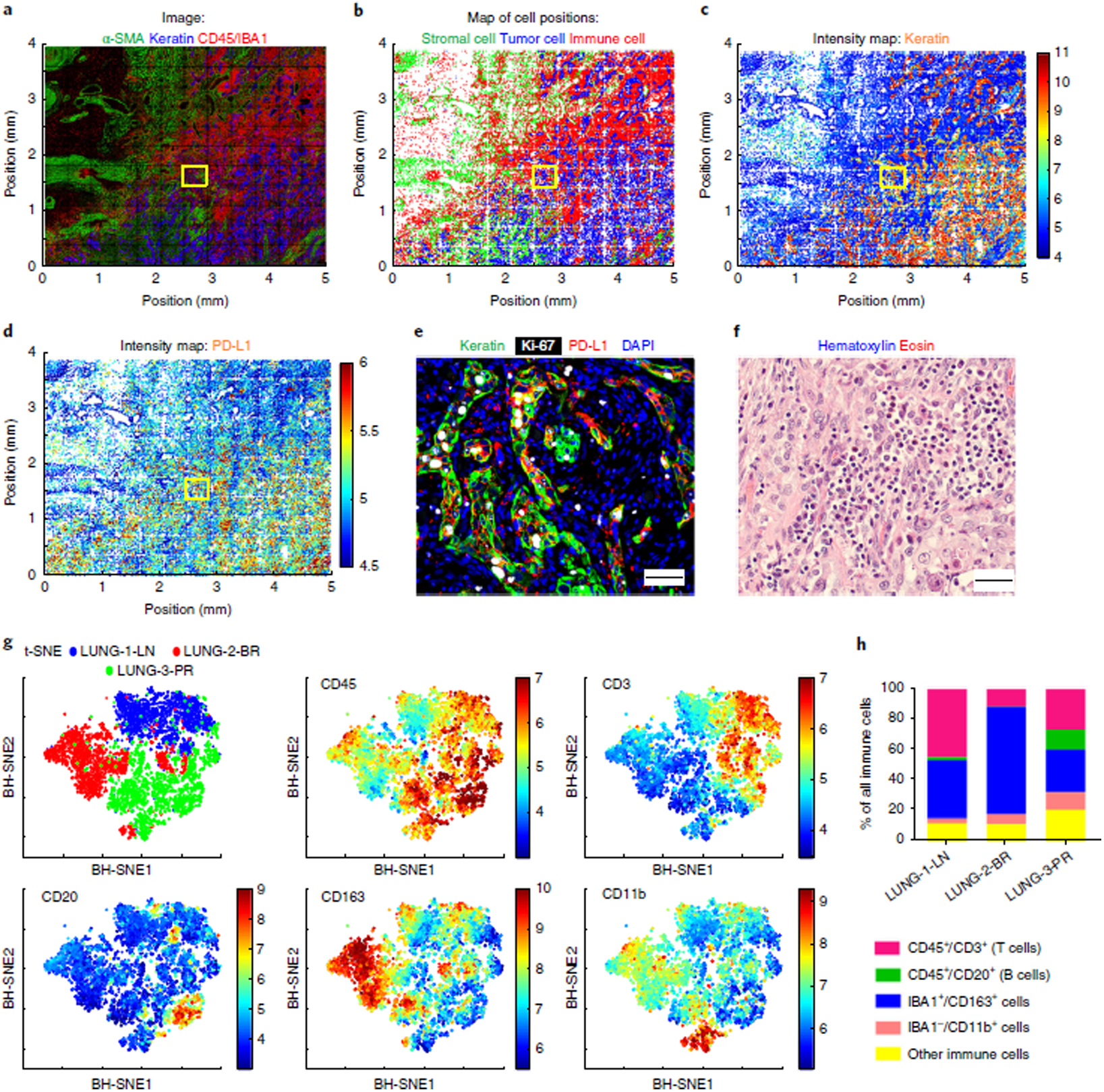
a, Montage of t-CyCIF immunofluorescence staining in a primary lung cancer resection sample (LUNG-3-PR) for α-SMA (green) for stromal myofibroblastic cells, pan-keratin (blue) for tumor cells, and CD45 or IBA1 (red) for immune cells. b, Corresponding map of cell positions, in which the intensity of the immunofluorescence data was integrated over each entire cell, with dots representing the computed centroid for each cell and colors representing the identity of each cell, using the same coding as in a. c,d, 2D spatially resolved intensity maps (red = high, blue = low) showing relative levels of expression of pan-keratin (c) and PD-L1 (d). e, A representative merged image of pan-keratin (green), Ki-67 (white), and PD-L1 (red) immunofluorescence corresponding to the yellow boxes in a–d. Scale bars, 50 μm. f, A representative image of H&E staining from a similar region in a serial section of LUNG-3-PR adjacent to that shown in e (scale bar, 20 μm). g, t-SNE plots for immune cell markers CD45, CD3, CD20, CD163, and CD11b from a random sampling of 2,000 immune cells from LUNG-1-LN, LUNG-2-BR, and LUNG-3-PR. The upper-left panel shows the discrete clustering of the immune populations from each resected specimen. The other panels show the intensity of staining for the indicated markers, where red = high and blue = low. h, Bar graph showing the percentage of each immune cell type relative to the total number of immune cells in the lung cancer samples (quantified in Supplementary Table 7). BH-SNE, Barnes–Hut stochastic neighbor embedding.

Fig. 6 |. Illustration of low-frequency CD45⁺/CD3⁺/FOXP3⁺/CD4⁻/CD8a⁺ T cells detected and confirmed by t-CyCIF.

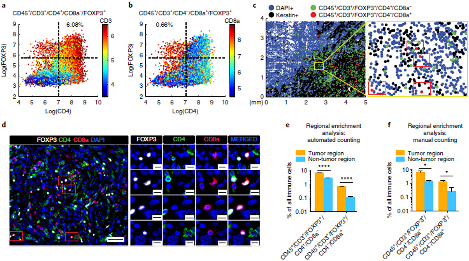
a,b, Scatter plots of CD4 and FOXP3 expression in lung cancer sample LUNG-3-PR with CD3 (a) and CD8a (b) expression mapped by color (red = high, blue = low). 6.08% of the immune cells were CD45⁺/CD3⁺/CD4⁺/FOXP3⁺/CD8a⁻, whereas 0.66% of the immune cells were CD45⁺/CD3⁺/CD4⁻/CD8a⁺/FOXP3⁺ (see Supplementary Table 8 for additional details). c, 2D dot plot map of the spatial distribution of CD45⁺/CD3⁺/FOXP3⁺/CD4⁺/CD8a⁻ cells (green dots) and CD45⁺/CD3⁺/FOXP3⁺/CD4⁻/CD8a⁺ cells (red dots) in LUNG-3-PR. We found four CD45⁺/CD3⁺/FOXP3⁺/CD4⁻/CD8a⁺ cells within the yellow framed region, and confirmed the presence of these four cells (red rectangles) by visual review of the t-CyCIF data (d; scale bars, 50 μm (left), 10 μm (right)). e,f, Bar graphs of regional enrichment analysis by automated counting (e) and manual counting (f) of t-CyCIF data showing that CD45⁺/CD3⁺/FOXP3⁺/CD4⁺/CD8a⁻ cells and CD45⁺/CD3⁺/FOXP3⁺/CD4⁻/CD8a⁺ cells were significantly enriched in the tumor region compared to the non-tumor region (see Supplementary Table 9 for additional details, including P values). Error bars represent s.e.m. *P < 0.05; ****P < 0.0001, t-test.

For ten critical immune markers, we explicitly tested the impact of order of addition and found that cycle number was not a critical variable. For example, Supplementary Table 5 shows data acquired from eight sequential sections of a human tonsil following addition of the same set of antibodies in either early or late cycles. Signal intensity was then measured from similar regions of the tissue, using the same image acquisition times. The correlation in staining intensity between early and late cycles was high for eight of the ten antibodies (CD14, CD163, CD20, CD3, CD4, CD8a, CD68, FOXP3, IBA1, and keratin; Supplementary Table 6 and Supplementary Figs. 11 and 12, but staining for anti-CD3 and anti-CD68 antibodies started to decrease after cycle 5 (Supplementary Table 6 and Supplementary Figs. 11 and 12). When anti-CD3 and anti-CD68 antibodies were used only in early cycles, there was little evidence of batch-to-batch variability (Supplementary Table 6). Moreover, even with the most problematic antibodies, the localization of the signal did not change, and only the intensity varied. These data are consistent with other t-CyCIF experiments showing that 15–20% of antibodies tested to date decrease in intensity with cycle number whereas 15–20% increase in intensity²⁰. In general, even when intensity varies across cycle number, we find that staining morphology is largely preserved. In a similar set of studies using the cyclic MxIF method, Gerdes et al.¹⁶ showed that ~12% of 59 antibodies tested exhibited some dependence on cycle number, and one antibody was extremely sensitive.

In the case of t-CyCIF, we find that reproducibility is high within a single slide and across slides processed in parallel. For most antibodies for which signal changes with cycle number, it is possible to control for intensity changes by processing all samples in parallel. Future work will focus on further mitigating the effects of cycle number by applying gating techniques and cell-calling algorithms that are less sensitive to absolute signal intensity, use of TMA-based calibration standards on each slide and identification of antibodies that are stable to changes in order of use.

When considered from the perspective of a single tissue sample, t-CyCIF can seem rather slow: in most cases, only one or two cycles (eight channels) of staining and imaging are performed per day. However, a single operator can process 30 or more slides in parallel and can image entire tissue sections of ≥4 cm². On a per-cell basis, throughput is higher than that for other multiplex tissue imaging methods, as well as single-cell technologies such as single-cell RNA-seq. For example, in the tissues described in the ‘Anticipated results’ section, ~10⁵ cells were quantified per sample. The analysis and interpretation of data from this many cells remains the most time-consuming aspect of high-dimensional tissue imaging and almost always exceeds the time required for data collection by several fold (estimates are provided in the ‘Timing’ section below). Note that all times in this paper are rough estimates influenced by the instrumentation available, the computing environment used (desktop, cluster, or cloud), the number of markers collected, and the questions being addressed. As instruments improve and analytical pipelines mature, we expect the speed of multiplex tissue imaging to increase greatly.

Materials

Biological materials

• FFPE tissue of interest. The procedure described here is compatible with most human and mouse tissues. In this protocol, we exemplify our approach using human tonsil FFPE tissue and three human lung cancer FFPE tissues (LUNG-1-LN: lung adenocarcinoma metastasis to lymph node; LUNG-2-BR: lung squamous cell carcinoma metastasis to brain; and LUNG-3-PR: primary lung squamous cell carcinoma), all of which were accessed from the archives of the Department of Pathology, Brigham and Women’s Hospital, Harvard Medical School ! CAUTION All experiments involving human tissues should be performed in accordance with the relevant guidelines established by local ethics committees and local biosafety guidelines for handling biohazardous materials. This study was approved by the institutional review boards (IRBs) of Brigham and Women’s Hospital and the Dana-Farber Cancer Institute, Harvard Medical School, as part of a discarded-tissue protocol for de-identified patient samples ▲CRITICAL Generally, optimal results are obtained when using freshly cut 5-μm FFPE sections mounted on glass slides. Unstained sections can be stored at room temperature (RT; 15–25 ° C) or 4 °C with the important caveat that a substantial decrease in signal can occur for some antibodies when staining is performed on slides that have been stored for several months, particularly those kept at RT.

Reagents

• Antibodies for t-CyCIF and IHC (see the antibodies used in this protocol in Table 2 and Supplementary Tables 2–4) ▲CRITICAL Store the antibodies according to the manufacturer’s instructions. In general, fluorophore-conjugated antibodies should be stored in the dark. For antibodies that should be stored at −20 °C according to the manufacturer’s instructions, we recommend dividing the stock into 25-μl aliquots to avoid freeze–thaw cycles.

• HistoGel (VWR, cat. no. HG-4000–012)

• Deionized water

• Formaldehyde (Thermo Fisher Scientific, cat. no. 28906)

• Formalin (Sigma-Aldrich, cat. no. HT501128–4L)

• Pierce 20× PBS (Thermo Fisher Scientific, cat. no. 28348)

• UltraPure glycerol (Life Technologies, cat. no. 15514011)

• Hydrogen peroxide solution (H₂O₂, 30% (wt/vol), ACS grade, including stannate-containing compounds and phosphorus-containing compounds to stabilize the solution; Sigma-Aldrich, cat. no. 216763–500ML) ! CAUTION Hydrogen peroxide is toxic; wear protective personal equipment, such as a lab coat, gloves, mask, and glasses.

• Sodium hydroxide (NaOH, Sigma-Aldrich, cat. no. 221465–500G) ! CAUTION Sodium hydroxide is toxic; wear protective personal equipment, such as a lab coat, gloves, mask, and glasses.

• Odyssey blocking buffer in PBS (500 ml; LI-Cor, cat. no. P/N 927–40003)

• Hoechst 33342 (25 mg; Cell Signaling Technology, cat. no. 4082)

• Bond dewax solution (Leica, cat. no. AR9222)

• Bond epitope retrieval solution 1 (ER1; Leica, cat. no. AR9961)

• HistoGel (VWR, cat. no HG-4000–012)

• Ethanol (Thermo Fisher Scientific, cat. no. 4355451)

Equipment

• Platinum coverslips (25 × 50 mm; VWR, cat. no. 48393–081)

• StainTray 10-slide tray (black; StatLab, cat. no. LWS10BK)

• Tissue-Tek vertical 24-slide rack (StatLab, cat. no. LWS2124)

• Tissue-Tek slide staining set (dishes and baths; StatLab, cat. no. LWS19)

• Damp paper towels (VWR, cat. no. 470308–268)

• Portable 20,000 Lux dimmable LED bright light panel (Amazon, cat. no. B078JCBW9S)

• Bond Universal Covertiles (Leica, cat. no. S21.4611)

• Bond RX machine (Leica, model no. 21.2701)

• T75 flasks (Fisher/Corning, cat. no. 353110)

• Falcon tube (15 ml; Fisher/Corning, cat. no. 352196)

• Graduated cylinders (100-ml, glass; StatLab, cat. no. LWG0726)

• Centrifuge tubes (15 and 50 ml; Corning, cat. nos. 430790 and 430808)

• Pipettes (5, 10, 25, and 50 ml; Corning, cat. nos. 4487, 4488, 4489, 4490)

• Standard micropipettes and tips

• Parafilm (VWR, cat. no. 291–1213)

Slide-scanning microscope

▲CRITICAL The procedures described in this work are optimized for the CyteFinder. We have also tested the IN Cell Analyzer and other instruments (see ‘Experimental design’ section).

• Slide-scanning microscope (CyteFinder; RareCyte, model no. 24-1001-000)

• Filter sets for the CyteFinder. The ‘DAPI channel’ for imaging Hoechst uses an excitation of 48 nm; the ‘488 channel’ has a 475-/28-nm excitation filter and a 525-n/48-nm emission filter; the ‘555 channel’ has a 542-/27-nm excitation filter and a 597-/45-nm emission filter; and the ‘647 channel’ has a 632-/22-nm excitation filter and a 679-/34-nm emission filter

• Filter sets for the IN Cell Analyzer 6000. ‘DAPI channel’ with 455-nm peak excitation/25-nm half-bandwidth, ‘488 channel’ with 525-nm peak excitation/10-nm half-bandwidth, ‘555 channel’ with 605-nm peak excitation/26-nm half-bandwidth, and ‘647 channel’ with 706.5-nm peak excitation/36-nm half-bandwidth

• Objective lenses for the CyteFinder: either a 10× (NA = 0.3) or 40× (NA = 0.6) long-working-distance objective can be used

• Objective lenses for the IN Cell Analyzer 6000: a 10× (NA = 0.3), 20× (NA = 0.75), 40× (NA = 0.95), or 60× (NA = 0.95) long-working-distance objective can be used

Software

• ImageJ (https://imagej.nih.gov/ij/); RRID: SCR_003070

• MATLAB (https://www.mathworks.com/products/matlab.html); RRID: SCR_001622

• ASHLAR (https://github.com/sorgerlab/ashlar); RRID: SCR_016266

• viSNE algorithms from the CYT single-cell analysis package were obtained from D. Pe’er’s laboratory at Columbia University⁹⁶ and were run with MATLAB R2017a

• X-shift: VorteX 29-Jun-2017-rev2 was obtained from G. Nolan’s laboratory at Stanford University School of Medicine⁹⁷ (https://github.com/nolanlab/vortex/releases)

• Venn diagrams are made using Venny 2.1, developed by J. Oliveros at the National Centre for Biotechnology (http://bioinfogp.cnb.csic.es/tools/venny/index.html)

• Aperio ImageScope software (Leica: https://www.leicabiosystems.com/digital-pathology/manage/aperio-imagescope/)

Reagent setup

PBS buffer solution (1×)

Combine 50 ml of Pierce 20× PBS with 950 ml of deionized water. 1× PBS buffer can be prepared in advance and stored at RT for several weeks.

Phosphate-buffered formaldehyde, 4% (wt/vol)

Combine 3 mL of 1× PBS with 1 mL of 16% (wt/vol) formaldehyde (Thermo Fisher Scientific, cat. no. 28906). Phosphate-buffered formaldehyde should be prepared immediately before use.

Hoechst solution

Dilute 25 mg of Hoechst 33342 in 10 ml of deionized water to make a 2.5 mg/ml stock solution and store it at 4 °C in the dark for up to 6 months. To make a working solution, dilute the stock solution in Odyssey blocking buffer (1:1,000 (vol/vol)) to stain the DNA and mark nuclei ▲CRITICAL Hoechst working solution should be prepared immediately before use.

NaOH solution, 1 M

Combine 2 g of sodium hydroxide with 50 ml of deionized water in a 50-ml centrifuge tube. Vortex the solution to allow the sodium hydroxide to dissolve completely. 1 M NaOH can be prepared in advance and stored at RT for several months.

Fluorophore bleaching solution

Combine 25 ml of 1× PBS, 4.5 ml of 30% (wt/vol) H₂O₂, and 0.8 ml of 1 M NaOH in a 50-ml centrifuge tube. The final working concentration is 4.5% (wt/vol) H₂O₂ and 20 mM NaOH in PBS. 30 ml of fluorophore bleaching solution is enough for four standard slides ▲CRITICAL Fluorophore bleaching solution should be prepared immediately before use.

Glycerol solution, 10% (vol/vol)

Combine 1 ml of UltraPure glycerol with 9 ml of 1× PBS in a 15-ml centrifuge tube. 10% (vol/vol) glycerol in PBS can be prepared in advance and stored at RT for several weeks.

Antibody mixture for t-CyCIF

Dilute antibodies of interest in Odyssey blocking buffer according to their optimal dilutions/concentrations (Supplementary Table 3). The antibody mixture can be prepared up to several hours before use and stored at 4 °C in the dark ▲CRITICAL Keep the antibody mixture at 4 °C or on ice.

Procedure

FFPE slide pretreatment, pre-staining, and background determination ● Timing 16–24 h

▲CRITICAL Slide pre-staining (blocking) and background signal determination are particularly important for tissues with high autofluorescence.

• 1Perform the FFPE slide pretreatment procedure. See Box 3 for our recommended procedure.

  ▲CRITICAL STEP We perform FFPE slide pretreatment—involving slide baking, dewaxing, antigen retrieval, and blocking—on a Leica Bond RX automated slide processor in this work. Similar instruments are manufactured by Ventana or Dako and are commonly found in histopathology core facilities. FFPE slide pretreatment can also be accomplished by performing manual dewaxing and antigen retrieval (e.g., microwaving slides in citrate buffer or using a pressure cooker)²⁰.

• 2Place slides flat in a transparent plastic container with the tissue sample facing up, and then gently pour fluorophore bleaching solution into the container to completely cover the tissue. Place the container between two LED light panels (one above and one below) at RT for 45 min.

  ▲CRITICAL STEP The pre-bleaching step is critical for reducing autofluorescence in the tissue and to inactivate the fluorophores of the secondary antibody from the pre-staining step.

  ▲CRITICAL STEP Light sources that produce excessive heat can damage tissues. LED light sources are therefore preferable, and large, flat LED panels are now readily available at low cost (see ‘Equipment’ section for our preferred light panel).

  ▲CRITICAL STEP Completely immerse the tissue sections in fluorophore bleaching solution. During the subsequent bleaching process, bubbles will appear and will gradually increase in size and number. This indicates that the oxidation reaction is proceeding as expected.

  ? TROUBLESHOOTING

• 3Wash the slides four times with 1× PBS at RT for 3–5 min per wash. Slides can be placed into a slide rack and lowered into a staining dish of PBS.
• 4Place the slides in the slide tray, cover the tissue with the secondary antibody solution used in the pretreatment step (see Box 3 and Table 2 for the antibodies used in this protocol), and incubate in the dark at 4 °C overnight to block non-specific binding.

  ▲CRITICAL STEP Place damp paper towels in the slide tray to maintain humidity and prevent evaporation of the antibody solution.

  ▲CRITICAL STEP Do not use a hydrophobic barrier pen on the slides, because we have found that this adversely affects subsequent cycles.

  ▲CRITICAL STEP Be careful not to scratch the tissue with the pipette tip when applying the antibody solution.

• 5Bleach the fluorophores for 45 min at RT as described in Step 2.
• 6Wash the slides four times with 1× PBS at RT for 3–5 min per wash.

  ▲CRITICAL STEP Wash the slides to remove the fluorophore bleaching solution completely, because this may affect subsequent t-CyCIF steps.

• 7Incubate the slides with Hoechst solution (2.5 μg/ml) in the dark at RT for 10 min.
• 8Wash the slides four times with 1× PBS at RT for 3–5 min per wash.
• 9Mount coverslips onto the slides with 200 μl of 10% (vol/vol) glycerol in 1× PBS to prevent dehydration during imaging. Carefully position the coverslips over the center of each slide and lower slowly onto the slide to avoid producing bubbles between the coverslip and the slide, and to prevent scratching of tissues. Do not allow the coverslip to hang over the edge of the slide. Dry excess liquid by gently pressing the long edges of the slide against a paper towel.

  ▲CRITICAL STEP Wet mounting and positioning of coverslips takes some practice, which should be initially undertaken using non-precious specimens.

• 10Load the slide into the slide scanner (CyteFinder) and image at four wavelengths to record the background signal.

  ▲CRITICAL STEP Typically, only a portion of each slide is covered in tissue and only this region should be scanned; it is important to save this ROI in the imaging software so that precisely the same region can be imaged in subsequent rounds of t-CyCIF.

  ▲CRITICAL STEP Check the images as they are being acquired and adjust exposure times to remain in a linear range.

  ? TROUBLESHOOTING

• 11After image acquisition, remove the coverslips by placing the slides in 1× PBS in a staining dish (which holds slides vertically) for 10 min and then slowly pulling the slides vertically out of the solution, allowing the coverslip to remain behind.

  ▲CRITICAL STEP De-coverslipping is a procedure that requires practice. Always allow coverslips to fall away through gravity. Do not push the coverslips, because this will scratch and damage the tissues. It may take >10 min for the coverslips to detach.

• 12Wash the slides four times with 1× PBS at RT for 3–5 min per wash.

  ■PAUSE POINT Slides can be stored in 1× PBS at 4 °C for several days. Make sure the entire tissue is covered in 1× PBS; otherwise, the tissue will dry out, producing poor results in subsequent staining steps.

Box 3 |. FFPE slide pretreatment in the Bond RX machine ● Timing 3 h.

Procedure

! CAUTION Follow local biosafety guidelines for handling of biohazardous materials.

▲CRITICAL Note that the FFPE slide pretreatment procedure described below involves baking, dewaxing, antigen retrieval, and blocking on a Bond RX automated slide processor; similar instruments are manufactured by Ventana or Dako and are commonly found in histopathology core facilities. Those steps can also be performed following manual dewaxing and antigen retrieval (e.g., microwaving slides in citrate buffer or using a pressure cooker)²⁰.

1. Create a protocol file named ‘t-CyCIF’ on the Bond RX automated slide processor with the following conditions.

   1. Bake FFPE slides at 60 °C for 30 min.
   2. Dewax by rinsing three times with 150 μl of preheated (60 °C) Bond dewax solution, followed by three rinses with 150 μl of 200 proof ethanol.
   3. Remove the Bond dewax solution. Add 150 μl of Bond ER1 solution for antigen retrieval and incubate at 99 °C for 20 min.
   4. Remove the Bond ER1 solution and block for 30 min with 150 μl of Odyssey blocking buffer at RT.
   5. Remove the blocking buffer and incubate with 150 μl of secondary antibody solution (see Table 2 for the antibodies used in this protocol) by incubating for 60 min at RT.
   6. Remove the secondary antibody solution and incubate with 150 μl of Hoechst solution for 30 min at RT.
      ▲CRITICAL STEP We recommend saving the protocol file in the Leica RX machine for future use.

2. Fill chamber 1 with 30 ml of 1× PBS.

3. Fill chamber 2 with 7 ml of Odyssey blocking buffer.

4. Fill chamber 3 with 2 ml of the appropriate secondary antibodies conjugated with Alexa Fluor 488, Alexa Fluor 555, or Alexa Fluor 647 diluted in Odyssey blocking buffer (1:1,000 (vol/vol)) (see Table 2 for the antibodies used in this protocol).

   ▲CRITICAL Before the first cycle of t-CyCIF, a pre-staining (blocking) step is performed by incubating tissues with a mixture of appropriate secondary antibodies to block non-specific binding sites in the tissue. Secondary antibodies are chosen on the basis of the species and isotypes of the unconjugated antibodies used in the first t-CyCIF cycle. Anti-rabbit Alexa Fluor 555 and anti-mouse Alexa Fluor 647 secondary antibodies were used in this study (Table 2).

   ▲CRITICAL Avoid using Alexa Fluor 546–, Alexa Fluor 568– or Alexa Fluor 594–conjugated secondary antibodies, because these fluorophores are resistant to bleaching.

5. Place chambers in the reagent tray and insert it into the Bond RX machine.

6. Create a new study on the Bond RX machine, select the ‘t-CyCIF’ file created in Step 1 as the protocol, add each slide to the study, and print labels for each FFPE slide. The Bond requires barcoded labels on all slides to process them.

   ▲CRITICAL STEP Center the slide stickers evenly, so that the Bond RX machine can scan the barcodes on the stickers correctly.

7. Open the lids of the reagent chambers and insert the reagent chamber tray into the Bond RX machine.

8. Place all labeled slides onto a slide tray, cover the slides with Bond Universal Covertiles, and insert the slide tray into the machine.

   ▲CRITICAL STEP Be sure to place the Covertiles right side up, using the ‘Leica’ etched into each Covertile as an orientation guide.

9. The Bond RX machine will scan the barcodes on the stickers of the slides and reagent chambers. Check the label readings by hovering the mouse over the slide labels. If all the slides have been recognized correctly, then click the ‘START’ button to run the protocol. This will dewax slides and perform antigen retrieval.

   ? TROUBLESHOOTING

10. Remove the slides from the Bond RX machine and place them into 1× PBS.

    ■PAUSE POINT Slides can be stored in 1× PBS at 4 °C for several days after processing on the Bond RX machine. Ensure that the entire tissue is completely covered in 1× PBS; otherwise, the tissue will dry out and yield poor results.

First round of t-CyCIF ● Timing 16–24 h

• 13Dilute up to three unconjugated primary antibodies from different species to the appropriate concentration in Odyssey blocking buffer (see Table 2 for the antibodies used in this protocol), cover all the tissue, and incubate in the dark at 4 °C overnight.

  ▲CRITICAL STEP In the first round of t-CyCIF, unconjugated primary antibodies can be used. As in conventional immunofluorescence, these antibodies must be from different species (e.g., rabbit, mouse, and rat) to allow for detection with species-specific secondary antibodies. The optimal dilution for primary antibodies must be optimized empirically; we usually test across a range of dilutions starting from 1:100 (vol/vol), guided by the manufacturer’s recommendations. The times listed for antibody incubation can be adjusted empirically; we use long incubations at 4 °C for convenience. See Lin et al.²⁰ and https://www.cycif.org/ (RRID: SCR_016267) for information on increasing the throughput of t-CyCIF experiments.

• 14Wash the slides four times with 1× PBS at RT for 3–5 min per wash.
• 15Cover the tissue with secondary antibodies and incubate in the dark at RT for 2 h.
• 16Incubate with Hoechst solution (2.5 μg/ml) in the dark at RT for 10 min.
• 17Wash the slides four times with 1× PBS at RT for 3–5 min per wash.
• 18Mount coverslips onto the slides with 200 μl of 10% (vol/vol) glycerol in PBS and image the saved ROI for each slide with the CyteFinder as described in Step 10.

  ▲CRITICAL STEP Use the saved ROI in the imaging software so that the exact same region of tissue is imaged for each t-CyCIF cycle.

  ? TROUBLESHOOTING

• 19After imaging, remove the coverslips as described in Step 11 and wash the slides four times with 1× PBS at RT for 3–5 min per wash.
• 20Perform fluorophore bleaching for 45 min at RT as described in Step 2.
• 21Wash the slides four times with 1× PBS at RT for 3–5 min per wash.

  ▲CRITICAL STEP Wash the slides thoroughly to remove fluorophore bleaching solution, because carryover can adversely affect subsequent t-CyCIF cycles.

  ■PAUSE POINT The slides can be stored in 1× PBS at 4 °C for several days. Make sure the entire tissue is covered in 1× PBS. Otherwise, the tissue may become dry and yield poor staining results.

Subsequent cycles of t-CyCIF ● Timing 16–24 h per cycle

▲CRITICAL The maximum number of t-CyCIF cycles depends on the tissue type, which is evaluated by counting nuclei in the Hoechst channel. We routinely perform >10 cycles for most tissue types and >20 cycles for some especially resilient tissues, such as tonsil.

• 22Dilute up to three antibodies conjugated with different fluorophores in Odyssey blocking buffer. Cover all tissue with antibody solution and incubate in the dark at 4 °C overnight.

  ▲CRITICAL STEP We typically use Alexa Fluor 488–, Alexa Fluor 555–, and Alexa Fluor 647–conjugated primary antibodies. Dilution is optimized empirically, starting from 1:100 (vol/vol).

  ▲CRITICAL STEP Avoid using Alexa Fluor 546–, Alexa Fluor 568–, and Alexa Fluor 594–conjugated secondary antibodies because these fluorophores are difficult to bleach.

• 23Wash the slides four times with 1× PBS at RT for 3–5 min per wash.
• 24Incubate with Hoechst solution (2.5 μg/ml) in the dark at RT for 10 min.
• 25Wash the slides four times with 1× PBS at RT for 3–5 min per wash.
• 26Mount coverslips onto slides with 200 μl of 10% (vol/vol) glycerol in PBS and image the saved ROI with the CyteFinder as described in Step 10.
• 27Remove the coverslips as described in Step 11.
• 28Wash the slides four times with 1× PBS at RT for 3–5 min per wash.
• 29Bleach the fluorophores for 45 min at RT as described in Step 2.
• 30Wash the slides four times with 1× PBS at RT for 3–5 min per wash.
• 31Repeat Steps 22–30 for each additional t-CyCIF cycle.

  ? TROUBLESHOOTING

Image processing ● Timing Variable

▲CRITICAL The data described here were obtained using pre-processing, registration, segmentation, and quantification software in ImageJ (scripts provided in Sorger Lab GitHub repository: https://github.com/sorgerlab/cycif). As noted in the Introduction, many alternative tools are available.

▲CRITICAL In Steps 32–34, change the parameters in each script to account for the directory and names of the image files, the start and end cycle numbers, and the number of rows and columns used to create montages.

• 32Run the ‘1_Macro-SAVEALLCYCLES.ijm’ script on ImageJ to perform background subtraction and flat-field correction and save .tiff images of individual tiles from the .rcpnl file generated by the CyteFinder for each cycle.
• 33Run the ‘2_Macro-imagereg-forRareCyte.ijm’ script to perform registration of each tile using the Hoechst signal and a rigid-body transformation algorithm. The registration information is applied to all channels of all images from each t-CyCIF cycle to generate a hyperstack of images from all cycles.
• 34Run the ‘3_Macro-CycIF-wholeslidequan.ijm’ script to segment cells using the Hoechst signal from the last cycle, measure the average intensity of each marker for each cell, and output the data as a .cvs file for each image tile.

  ▲CRITICAL STEP Use the Hoechst image from the final cycle to generate a mask.

High-dimensional data analysis and visualization ● Timing Variable

▲CRITICAL All MATLAB scripts used in this section are available in the Sorger Lab GitHub repository (https://github.com/sorgerlab/cycif). As noted in the Introduction, many alternative tools and programming languages can be used.

• 35Run ‘CycIF_readwholeslide.m’ to import the single-cell data generated by Step 34 into MATLAB R2017a.
• 36Identify specific cell populations by manual gating. Set cutoff values for each marker by having a trained user review intensity distributions and fluorescence images.

  ▲CRITICAL STEP Alternatively, GMM can be fitted using the expectation maximization (EM) algorithm in MATLAB. For each GMM, at least 80 different initial guesses are used as starting points for the EM algorithm to find the maximum-likelihood fit.

• 37Generate heatmaps based on the intensity data for a particular marker and the location information of the cells (Xt, Yt as transformed x-y location of each cells) using MATLAB. Dot plots can be generated by applying cutoff values for particular markers.
• 38Generate cluster plots, cross-correlation plots, and scatter plots from intensity data using MATLAB.
• 39Perform t-SNE analysis using the viSNE implementation from the CYT single-cell analysis package⁹⁶ and run in MATLAB.
• 40(Optional) Perform X-shift analysis using VorteX 29-Jun-2017-rev2 from the Nolan lab (https://github.com/nolanlab/vortex/releases/tag/29-Jun-2017) (plots not shown).
• 41(Optional) Generate Venn diagrams using the online Venny 2.1 tool from the Centro Nacional de Biotecnología (CNB) in Spain (http://bioinfogp.cnb.csic.es/tools/venny/) (diagrams not shown).

Troubleshooting

Troubleshooting advice can be found in Table 3.

Table 3 |.

Troubleshooting table

Step	Problem	Possible reason	Solution
2	No bubbles in fluorophore bleaching solution	Incorrect lighting source or bleaching solution used	Use white LED light for fluorophore inactivation; use freshly made bleaching solution
10	Blurry images	The slide is not flat on microscope stage or there are bubbles between the slide and the coverslip	Examine the slide holder for precipitate and remove it; ensure slides are loaded properly in the slide holder; re-coverslip; adjust the focus points
18	Weak signal	Low signal can occur because of low-level antigen expression. Direct immunofluorescence using conjugated antibodies does not provide the signal amplification that can be generated in indirect immunofluorescence	Increase the exposure time while acquiring the image; increase the antibody concentration during the staining step; use the corresponding unconjugated antibodies in the first round instead of the conjugated antibody to see if signal amplification from indirect immunofluorescence improves signal; if necessary, find an alternative antibody
	Saturated signal	Abundant antigen in sample or excessive amount of antibody. Exposure time too long	Decrease the antibody concentration used during the staining step; decrease the incubation time of the sample with antibody; decrease the exposure time during image acquisition
31	Cell loss	Difficult tissue type (very low cell density). Insufficient tissue fixation. Damage from t-CyCIF procedure (e.g., rough handling of samples during washing)	Check pre-analytical variables. Be cautious in handling of samples during application of antibodies and washing steps, as well as during manipulation of coverslips
	Signal present after fluorophore bleaching step	Insufficient fluorophore inactivation	Avoid Alexa Fluor 546-, Alexa Fluor 568-, and Alexa Fluor 594-conjugated antibodies because they are difficult to inactivate; dilute conjugated antibodies further; extend fluorophore bleaching time; check that light is hitting the sample
Box 3, step 9	Leica Bond RX machine fails to start	Incorrect setup of machine	Read the manufacturer’s instructions; check the protocol and reagent setup carefully; contact vendor

Timing

Steps 1–12, FFPE slide pretreatment, pre-staining, and background recording: 16–24 h

Steps 13–21, first round of t-CyCIF: 16–24 h

Steps 22–31, subsequent cycles of t-CyCIF: 16–24 h per cycle

Steps 32–34, image processing: variable (~8 h computing time for a 12-GB dataset of images using a computer with 32 GB of RAM, or one slide using the 16-marker panel described here)

Steps 35–41, high-dimensional data analysis and visualization: variable (several days to weeks, depending on the research question and the investigators’ computational expertise)

Box 1, creating FFPE cell line microarrays for antibody testing: 17 h

Box 3, FFPE slide pretreatment in Bond RX machine: 3 h

Anticipated results

Immune profiling of lung cancer samples

We analyzed three human primary and metastatic lung carcinoma specimens to demonstrate the performance of the immune profiling panels validated and assembled through this protocol. The tissues represent contexts typically encountered when evaluating malignancies; a lymph node metastasis (LUNG-1-LN), a brain metastasis (LUNG-2-BR), and a primary lung tumor (LUNG-3-PR), each from a different patient. We performed nine-cycle t-CyCIF in parallel on the three specimens, followed by image segmentation, computational analysis, and visual review by board-certified pathologists (Figs. 5–8, Supplementary Figs. 13–23, Supplementary Tables 7–10 and Supplementary Movie 2). We then enumerated and mapped high- and low-frequency immune cell types, visualizing their spatial distribution within the tumors.

Fig. 8 |. Systematic automated identification of rare subpopulations using t-CyCIF.

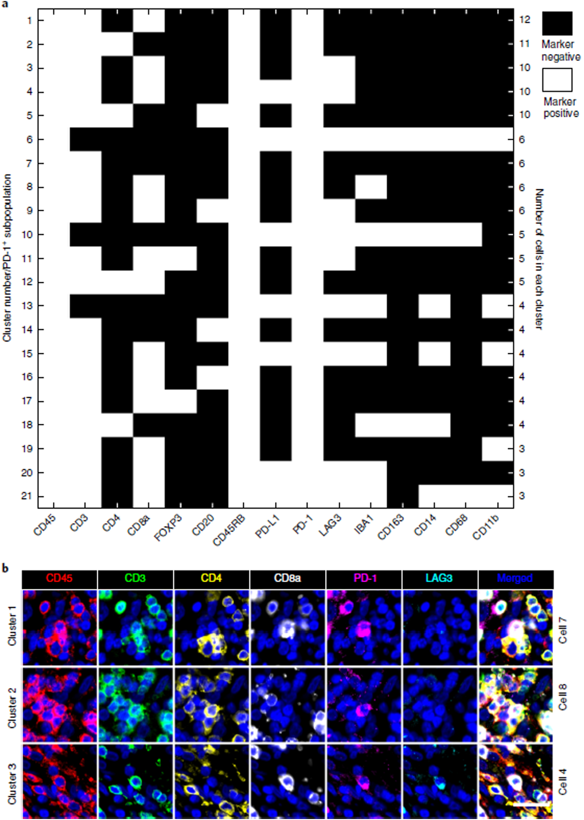
a, All PD-1⁺ cells (n = 273) from LUNG-3-PR were further separated using binary gating of all 15 immune markers. 21 putative subpopulations comprising three or more cells are shown. Cluster 3 is the subpopulation with PD-1⁺/LAG3⁺/CD8a⁺/CD3⁺ (described by visual review of scatter plots in Fig. 7). Images of all 125 cells binned into putative rare cell clusters 1 through 21 are shown in Supplementary Figs. 17–22. Supplementary Table 10 indicates whether visual review of the images by a trained pathologist was deemed to be consistent or inconsistent with the automated calls. Nine of the 21 clusters (1–4, 6, 8, 10, 11, and 17) were validated by visual review (38 of 125 individual rare cell calls). b, A gallery of images of individual markers from single cells from clusters 1 (CD45⁺/CD45RB⁺/CD3⁺/CD8a⁺/PD1⁺), 2 (CD45⁺/CD45RB⁺/CD3⁺/CD4⁺/PD1⁺), and 3 (CD45⁺/CD45RB⁺/CD3⁺/CD8a⁺/PD1⁺/LAG3⁺) are shown (with the exception of CD45RB). Images are shown for representative cells from each of these three clusters (scale bar, 25 μm).

The antibodies described in Supplementary Table 3 generated staining at intensities sufficiently above background to enable both manual and automated analysis. Manual review of images overlaid with segmentation masks revealed an overall accuracy of 80 ± 2% for computer-based cell identification, with visual analysis by a pathologist serving as the gold standard. We identified three types of computer-based segmentation errors: cells that were missed by the segmentation algorithm, fusion of two or more cells into a single segmented entity, and splitting of a single cell into two or more entities (Supplementary Fig. 9). Segmentation accuracy was similar in cancer samples and tonsil, but the types of errors differed with the sample. For example, artifactual fusion of densely packed lymphocytes in tonsil was common, whereas tumor cells in lung cancer specimens (which are larger than lymphocytes) tended to be split. We do not yet know whether these errors are random or systemic, and their effects on the accuracy of cell enumeration have not been evaluated. As noted in the ‘Experimental design’ section, the segmentation methods we applied are standard functions in ImageJ. More sophisticated segmentation algorithms using machine learning or multiple-features approaches (including nuclear, cytosolic, or membrane markers) would probably improve segmentation accuracy. Machine learning from pixel-level data—which avoids the need for image segmentation altogether and has been shown to yield superhuman performance in other medical imaging applications¹⁰³—is another possibility.

The panels we used were 20-plex with the inclusion of tumor and stromal markers (Table 2, Supplementary Table 3). 37 of these antigen-defined states comprise >0.5% of the total immune cell population in primary lung tumor LUNG-3-PR (the tumor type used as a reference in the current work), and 19 of these states are commonly encountered immune cell subtypes (Supplementary Fig. 1). In Fig. 5a, we show the immunofluorescence signal from a section of LUNG-3-PR that demonstrates the expression of four antigens: α-SMA (green), pan-keratin (blue), and CD45 or IBA1 (both red). A yellow box highlights a frame shown at high power in Fig. 5e, which depicts a representative merged image of pan-keratin (green), Ki-67 (white), and PD-L1 (red). An image from this region of an H&E stain from an adjacent serial section is also shown (Fig. 5f). To generate a map of cell positions, we integrated staining intensity over each successfully segmented cell across the image (following background subtraction) and used this information to call out distinct cell types: we labeled α-SMA⁺ cells as stromal cells, pan-keratin⁺ cells as tumor cells, and CD45⁺ or IBA1⁺ cells as immune cells. Dots mark the computed centroid of each cell, and colors represent each cell’s identity (Fig. 5b and Supplementary Fig. 14). In Figs. 6 and 7, we use multiple markers to define distinct cell states and present their locations in cell position plots. To facilitate visualization and assessment of the relative expression levels of individual antigens, we also generated intensity maps across the image. Maps are shown for keratin in Fig. 5c and for PD-L1 in Fig. 5d. The maps reveal substantial spatial heterogeneity of PD-L1 expression in the tumor cell compartment (Fig. 5d,e), suggesting dynamic and variable effects on immune surveillance. We also found that proliferating tumor cells, immune cells, and fibroblast populations were unevenly distributed, revealing additional forms of heterogeneity.

Fig. 7 |. Illustration of low-frequency CD45⁺/CD3⁺/PD-1⁺/LAG3⁺ T cells detected and confirmed by t-CyCIF.

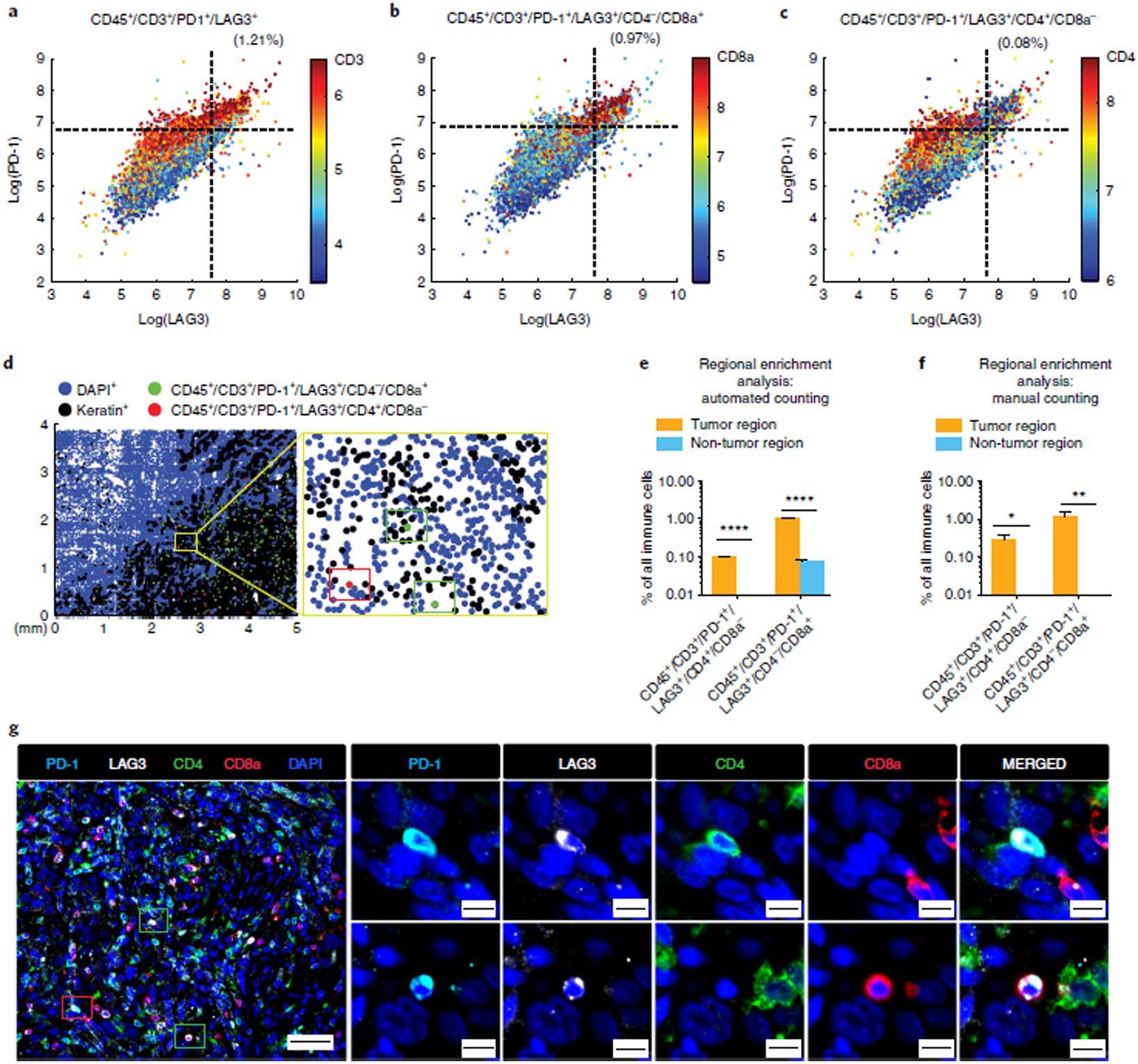
a–c, Scatter plots of LAG3 and PD-1 expression in LUNG-3-PR with CD3 (a), CD8a (b), and CD4 (c) expression mapped by color (red = high, blue = low). 2.49% of the immune cells were CD45⁺/CD3⁺/PD-1⁺, 1.21% of the immune cells were CD45⁺/CD3⁺/PD-1⁺/LAG3⁺, 0.97% of the immune cells were CD45⁺/CD3⁺/PD-1⁺/LAG3⁺/CD4⁻/CD8a⁺ and 0.08% of immune cells were CD45⁺/CD3⁺/PD-1⁺/LAG3⁺/CD4⁺/CD8a⁻ (see Supplementary Table 8 for details). d, 2D dot plot map of the spatial distribution of CD45⁺/CD3⁺/PD-1⁺/LAG3⁺/CD4⁻/CD8a⁺ cells (green dots) and CD45⁺/CD3⁺/PD-1⁺/LAG3⁺/CD4⁺/CD8a⁻ cells (red dots) in LUNG-3-PR. d,g, We found one CD45⁺/CD3⁺/PD-1⁺/LAG3⁺/CD4⁺/CD8a⁻ cell and two CD45⁺/CD3⁺/PD-1⁺/LAG3⁺/CD4⁻/CD8a⁺ cells in the yellow framed region (d, left; closeup on right) and confirmed the presence of these T-cell subpopulations by visual review of the t-CyCIF data (g), with the two different cell subpopulations indicated by red and green rectangles, respectively. (scale bars, 50 μm i(left), 10 μm (right)). e,f, Bar graphs showing regional enrichment analysis by automated counting (e) and by manual counting (f) of t-CyCIF data showing that CD45⁺/CD3⁺/PD-1⁺/LAG3⁺/CD4⁺/CD8a⁻ cells and CD45⁺/CD3⁺/PD-1⁺/LAG3⁺/CD4⁻/CD8a⁺ cells were significantly enriched in the tumor region compared to the non-tumor region (see Supplementary Table 9 for details, including P values). Error bars represent s.e.m. *P < 0.05; **P < 0.01; ****P < 0.0001, t-test.

We used t-SNE^1,3 to visualize and characterize the immune cell infiltrates from the tumor sections. t-SNE projects the 15D vectors of integrated staining intensity for each cell onto two dimensions in a manner that optimally preserves high-dimensional relationships. We performed t-SNE on 2,000 randomly selected immune cells from each of the three lung cancer specimens (Fig. 5g and Supplementary Fig. 15). This revealed clustering of immune cell populations by specimen and reflects marked specimen-specific differences in resident immune cell populations. When we projected the levels of expression of specific immune cell markers onto the t-SNE plots, we found that the LUNG-2-BR had few CD8⁺ T cells but many myeloid-derived immune cells (IBA1⁺/CD163⁺). By contrast, LUNG-3-PR was enriched in B cells (CD45⁺/CD20⁺) and T_reg cells (CD45⁺/CD3⁺/CD4⁺/FOXP3⁺). LUNG-1-LN was enriched specifically in CD45⁺/CD3⁺/CD8⁺ T cells (Fig. 5g,h and Supplementary Table 8). Thus, the immune environments of these tumors are very different, presumably reflecting tumor-intrinsic differences as well as differences in the location of the tumor at the time of resection.

Identifying and mapping low-frequency immune cell types

Many aspects of the tumor immune microenvironment remain enigmatic. A comprehensive understanding of the effects of the microenvironment on tumorigenesis and on response to therapy would probably involve characterizing the prevalence and locations of both high- and low-frequency immune cell populations. Highly multiplexed imaging is a powerful way to enumerate rare cell types because it provides data on cell morphology and environment as well as differentiation marker expression. Moreover, cells that are outliers in biomarker distributions can be revisited for visual re-review to confirm their presence and, potentially, to perform additional t-CyCIF staining. By contrast, re-review is not possible with flow cytometry data.

In our samples, multi-axis scatter plots of the three lung cancer specimens revealed three very-low-frequency immune cell populations: (i) CD8-expressing FOXP3⁺ T_reg cells (CD45⁺/CD3⁺/CD4⁻/CD8a⁺/FOXP3⁺ cells), which represented 0.01–0.66% of all immune cells; (ii) CD8-expressing LAG3/PD-1 double-positive T cells (CD45⁺/CD3⁺/CD4⁻/CD8a⁺/PD-1⁺/LAG3⁺ cells), which represented 0.01–0.97% of all immune cells; and (iii) CD4-expressing LAG3/PD-1 double-positive T cells (CD45⁺/CD3⁺/CD4⁺/CD8a⁻/PD-1⁺/LAG3⁺ cells), which represented 0.03–0.08% of all immune cells (Figs. 6 and 7, Supplementary Figs. 16 and 17, and Supplementary Table 8).

CD8-expressing FOXP3⁺ T_reg cells (CD45⁺/CD3⁺/CD4⁻/CD8a⁺/FOXP3⁺ cells) have been reported previously in both human and mouse lymph nodes, spleen, and blood, as well as in prostate cancer and hepatocellular carcinoma, and have been implicated in immune evasion and consequent disease progression^104–106. We confirmed by visual review the presence of small round cells with lymphocyte morphology that were clearly positive for CD45, CD3, FOXP3, and CD8 (marked with red dots and boxes in Fig. 6c,d), and negative for CD4. The presence of nearby cells staining positive for CD4 (marked in green) provided an internal positive control for CD4 staining. Compared to directly adjacent non-neoplastic lung tissue in the histologic section, both automated and manual analysis showed that this rare cell population was sixfold enriched in the tumor component (P < 0.0001; t-test). Conventional T_reg cells (which are FOXP3⁺/CD4⁺/CD8⁻) were also enriched in the tumor region, but to a lesser extent (2.3-fold; P < 0.001; t-test) (Fig. 6e,f and Supplementary Table 9).

Similarly, double-positive PD-1/LAG3 cells (CD45⁺/CD3⁺/CD4⁻/CD8a⁺/PD-1⁺/LAG3⁺ cells and CD45⁺/CD3⁺/CD4⁺/CD8a⁻/PD-1⁺/LAG3⁺ cells) were substantially enriched in the tumor domain. The ~1% of immune cells that were CD8⁺/PD-1⁺/LAG3⁺ were 14-fold more abundant in the tumor region (P < 0.0001; t-test) and the ~0.1% of immune cells that were CD4⁺/PD⁻1⁺/LAG3⁺ were found nearly exclusively in the tumor (P < 0.0001; t-test) (Fig. 7 and Supplementary Table 9). CD8⁺ T cells double-positive for PD-1 and LAG3 have been described previously in tumor-bearing animal models and shown to have an exhausted phenotype¹⁰⁷. They have also been found in human ovarian and triple-negative breast cancer resection specimens^108,109. However, the rarer CD4⁺ subtype is largely uncharacterized.

Multiplex imaging can also be used to identify truly rare cells. A surprising number of marker combinations that are currently either undescribed in the literature or only recently found can be observed in tissue biopsies¹¹⁰. For example, use of a systematic automated assessment of PD-1⁺ cells in the LUNG-3-PR specimen revealed the presence of up to 125 PD-1⁺ cells with one of 21 different marker combinations at a frequency of 3 cells per 2,000 or greater (Fig. 8). A trained pathologist reviewed galleries of 125 rare cell images across 15 immune cell markers (LAG3, PD-1, CD45RB, CD3, PD-L1, CD4, CD45, CD8a, CD163, CD68, CD14, CD11b, FOXP3, IBA1, and CD20) (Supplementary Figs. 17–23). The staining pattern could be confirmed for 38 cells, representing nine different marker combinations; in other cases, the data were unclear or cells had been fused during automated segmentation (Supplementary Table 10). This approach demonstrates the utility of combining automated identification methods that screen for potentially interesting biomarker combinations with visual review of immunofluorescence by human experts. Whether the rare immune cells represent intermediates in the differentiation of known cell types or have unique and undescribed functions remains to be determined.

Together, the data presented in this section show how multiplexed tissue imaging can be used to enumerate common, low-frequency, and very rare immune cell subtypes in stromal and tumor tissue. In this application, imaging has two advantages over flow cytometry: (i) the locations of cell types are preserved with respect to each other and the overall architecture of the tissue or tumor, and (ii) visual review can be used to confirm that outliers in marker distributions in fact represent cells in which the markers have the expected spatial distribution, thereby increasing confidence that the cell type is real. More broadly, the use of multiplexed, spatially resolved tissue imaging offers great potential for providing unprecedented insights into patient stratification^8,39, tissue architecture^8,19,20,67, and fundamental aspects of cellular biology.

Fig. 3 |. Validation of antibodies for immune profiling by comparison to clinical-grade antibodies.

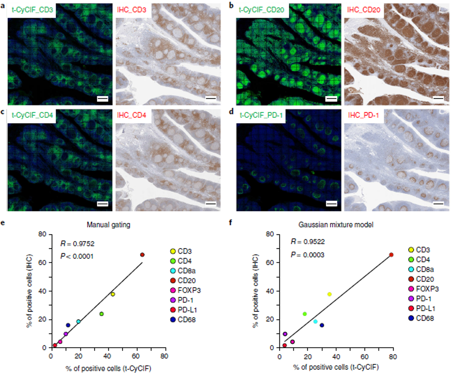
a–d, Representative images for t-CyCIF and IHC are shown for CD3 (a), CD20 (b), CD4 (c), and PD-1 (d) in human FFPE tonsil sections (scale bars, 500 μm). e,f, Correlation plots comparing the percentage of positive cells detected by t-CyCIF and IHC for each immune marker. Positive cells from the t-CyCIF data were identified using either manual gating (e) or GMM analysis (f), and thresholds for positive cells in IHC were set using Aperio ImageScope software. Similar plots for CD8a, FOXP3, PD-L1, and CD68 are presented in Supplementary Fig. 10.

References

- 1.Cyriac G & Gandhi L Emerging biomarkers for immune checkpoint inhibition in lung cancer. Semin. Cancer Biol 52, 269–277 (2018). [DOI] [PubMed] [Google Scholar]
- 2.Epstein JI, Egevad L, Humphrey PA, Montironi R & Members of the ISUP Immunohistochemistry in Diagnostic Urologic Pathology Group. Best practices recommendations in the application of immunohistochemistry in the prostate: report from the International Society of Urologic Pathology consensus conference. Am. J. Surg. Pathol 38, e6–e19 (2014). [DOI] [PubMed] [Google Scholar]
- 3.Falcon BL et al. High-content multiplexed tissue imaging and quantification for cancer drug discovery. Drug Discov. Today 18, 510–522 (2013). [DOI] [PubMed] [Google Scholar]
- 4.Bodenmiller B Multiplexed epitope-based tissue imaging for discovery and healthcare applications. Cell Syst. 2, 225–238 (2016). [DOI] [PubMed] [Google Scholar]
- 5.Carvajal-Hausdorf DE, Schalper KA, Neumeister VM & Rimm DL Quantitative measurement of cancer tissue biomarkers in the lab and in the clinic. Lab. Invest 95, 385–396 (2015). [DOI] [PMC free article] [PubMed] [Google Scholar]
- 6.Giesen C et al. Highly multiplexed imaging of tumor tissues with subcellular resolution by mass cytometry. Nat. Methods 11, 417–422 (2014). [DOI] [PubMed] [Google Scholar]
- 7.Angelo M et al. Multiplexed ion beam imaging of human breast tumors. Nat. Med 20, 436–442 (2014). [DOI] [PMC free article] [PubMed] [Google Scholar]
- 8.Keren L et al. A structured tumor-immune microenvironment in triple negative breast cancer revealed by multiplexed ion beam imaging. Cell 174, 1373–1387.e19 (2018). [DOI] [PMC free article] [PubMed] [Google Scholar]
- 9.Decalf J, Albert ML & Ziai J New tools for pathology: a user’s review of a highly multiplexed method for in situ analysis of protein and RNA expression in tissue. J. Pathol 247, 650–661 (2018). [DOI] [PubMed] [Google Scholar]
- 10.Glass G, Papin JA & Mandell JW SIMPLE: a sequential immunoperoxidase labeling and erasing method. J. Histochem. Cytochem 57, 899–905 (2009). [DOI] [PMC free article] [PubMed] [Google Scholar]
- 11.Tóth ZE & Mezey E Simultaneous visualization of multiple antigens with tyramide signal amplification using antibodies from the same species. J. Histochem. Cytochem 55, 545–554 (2007). [DOI] [PubMed] [Google Scholar]
- 12.Pirici D et al. Antibody elution method for multiple immunohistochemistry on primary antibodies raised in the same species and of the same subtype. J. Histochem. Cytochem 57, 567–575 (2009). [DOI] [PMC free article] [PubMed] [Google Scholar]
- 13.Remark R et al. In-depth tissue profiling using multiplexed immunohistochemical consecutive staining on single slide. Sci. Immunol 1, aaf6925(2016). [DOI] [PMC free article] [PubMed] [Google Scholar]
- 14.Goltsev Y et al. Deep profiling of mouse splenic architecture with CODEX multiplexed imaging. Preprint at bioRxiv, 10.1101/203166 (2017). [DOI] [PMC free article] [PubMed] [Google Scholar]
- 15.Wang Y et al. Rapid sequential in situ multiplexing with DNA exchange imaging in neuronal cells and tissues. Nano Lett. 17, 6131–6139 (2017). [DOI] [PMC free article] [PubMed] [Google Scholar]
- 16.Gerdes MJ et al. Highly multiplexed single-cell analysis of formalin-fixed, paraffin-embedded cancer tissue. Proc. Natl. Acad. Sci. USA 110, 11982–11987 (2013). [DOI] [PMC free article] [PubMed] [Google Scholar]
- 17.Schubert W et al. Analyzing proteome topology and function by automated multidimensional fluorescence microscopy. Nat. Biotechnol 24, 1270–1278 (2006). [DOI] [PubMed] [Google Scholar]
- 18.Friedenberger M, Bode M, Krusche A & Schubert W Fluorescence detection of protein clusters in individual cells and tissue sections by using toponome imaging system: sample preparation and measuring procedures. Nat. Protoc 2, 2285–2294 (2007). [DOI] [PubMed] [Google Scholar]
- 19.Hillert R et al. Large molecular systems landscape uncovers T cell trapping in human skin cancer. Sci. Rep 6, 19012(2016). [DOI] [PMC free article] [PubMed] [Google Scholar]
- 20.Lin J-R et al. Highly multiplexed immunofluorescence imaging of human tissues and tumors using t-CyCIF and conventional optical microscopes. Elife 7, e31657(2018). [DOI] [PMC free article] [PubMed] [Google Scholar]
- 21.Wählby C, Erlandsson F, Bengtsson E & Zetterberg A Sequential immunofluorescence staining and image analysis for detection of large numbers of antigens in individual cell nuclei. Cytometry 47, 32–41 (2002). [PubMed] [Google Scholar]
- 22.Ståhl PL et al. Visualization and analysis of gene expression in tissue sections by spatial transcriptomics. Science 353, 78–82 (2016). [DOI] [PubMed] [Google Scholar]
- 23.Lee JH et al. Highly multiplexed subcellular RNA sequencing in situ. Science 343, 1360–1363 (2014). [DOI] [PMC free article] [PubMed] [Google Scholar]
- 24.Lee JH et al. Fluorescent in situ sequencing (FISSEQ) of RNA for gene expression profiling in intact cells and tissues. Nat. Protoc 10, 442–458 (2015). [DOI] [PMC free article] [PubMed] [Google Scholar]
- 25.Larsson C, Grundberg I, Söderberg O & Nilsson M In situ detection and genotyping of individual mRNA molecules. Nat. Methods 7, 395–397 (2010). [DOI] [PubMed] [Google Scholar]
- 26.Chen KH, Boettiger AN, Moffitt JR, Wang S & Zhuang X RNA imaging. Spatially resolved, highly multiplexed RNA profiling in single cells. Science 348, aaa6090(2015). [DOI] [PMC free article] [PubMed] [Google Scholar]
- 27.Moffitt JR et al. High-performance multiplexed fluorescence in situ hybridization in culture and tissue with matrix imprinting and clearing. Proc. Natl. Acad. Sci. USA 113, 14456–14461 (2016). [DOI] [PMC free article] [PubMed] [Google Scholar]
- 28.Stewart JP et al. Standardising RNA profiling based biomarker application in cancer-The need for robust control of technical variables. Biochim. Biophys. Acta 1868, 258–272 (2017). [DOI] [PubMed] [Google Scholar]
- 29.True LD Methodological requirements for valid tissue-based biomarker studies that can be used in clinical practice. Virchows Arch. 464, 257–263 (2014). [DOI] [PMC free article] [PubMed] [Google Scholar]
- 30.Bordeaux J et al. Antibody validation. BioTechniques 48, 197–209 (2010). [DOI] [PMC free article] [PubMed] [Google Scholar]
- 31.Srivastava S, Ghosh S, Kagan J & Mazurchuk R The making of a PreCancer atlas: promises, challenges, and opportunities. Trends Cancer 4, 523–536 (2018). [DOI] [PubMed] [Google Scholar]
- 32.Coy S et al. Multiplexed immunofluorescence reveals potential PD-1/PD-L1 pathway vulnerabilities in craniopharyngioma. Neuro Oncol. 20, 1101–1112 (2018). [DOI] [PMC free article] [PubMed] [Google Scholar]
- 33.Dunn IF et al. Mismatch repair deficiency in high-grade meningioma: a rare but recurrent event associated with dramatic immune activation and clinical response to PD-1 blockade. JCO Precis. Oncol 10.1200/PO.18.00190 (2018). [DOI] [PMC free article] [PubMed] [Google Scholar]
- 34.Ke R et al. In situ sequencing for RNA analysis in preserved tissue and cells. Nat. Methods 10, 857–860 (2013). [DOI] [PubMed] [Google Scholar]
- 35.Krzywkowski T & Nilsson M Padlock probes to detect single nucleotide polymorphisms. Methods Mol. Biol 1649, 209–229 (2018). [DOI] [PubMed] [Google Scholar]
- 36.Krzywkowski T, Hauling T & Nilsson M In situ single-molecule RNA genotyping using padlock probes and rolling circle amplification. Methods Mol. Biol 1492, 59–76 (2017). [DOI] [PubMed] [Google Scholar]
- 37.Surrette C et al. Microfluidic tissue mesodissection in molecular cancer diagnostics. SLAS Technol. 22, 425–430 (2017). [DOI] [PubMed] [Google Scholar]
- 38.Schulz D et al. Simultaneous multiplexed imaging of mRNA and proteins with subcellular resolution in breast cancer tissue samples by mass cytometry. Cell Syst. 6, 531(2018). [DOI] [PMC free article] [PubMed] [Google Scholar]
- 39.Tsujikawa T et al. Quantitative multiplex immunohistochemistry reveals myeloid-inflamed tumor-immune complexity associated with poor prognosis. Cell Rep. 19, 203–217 (2017). [DOI] [PMC free article] [PubMed] [Google Scholar]
- 40.Wei SC, Duffy CR & Allison JP Fundamental mechanisms of immune checkpoint blockade therapy. Cancer Discov. 8, 1069–1086 (2018). [DOI] [PubMed] [Google Scholar]
- 41.Sharma P & Allison JP Immune checkpoint targeting in cancer therapy: toward combination strategies with curative potential. Cell 161, 205–214 (2015). [DOI] [PMC free article] [PubMed] [Google Scholar]
- 42.Wong PF et al. Multiplex quantitative analysis of tumor-infiltrating lymphocytes and immunotherapy outcome in metastatic melanoma. Clin. Cancer Res 25, 2442–2449 (2019). [DOI] [PMC free article] [PubMed] [Google Scholar]
- 43.Jerby-Arnon L et al. A cancer cell program promotes T cell exclusion and resistance to checkpoint blockade. Cell 175, 984–997.e24 (2018). [DOI] [PMC free article] [PubMed] [Google Scholar]
- 44.Socinski MA et al. Atezolizumab for first-line treatment of metastatic nonsquamous NSCLC. N. Engl. J. Med 378, 2288–2301 (2018). [DOI] [PubMed] [Google Scholar]
- 45.Carbone DP et al. First-line nivolumab in stage IV or recurrent non-small-cell lung cancer. N. Engl. J. Med 376, 2415–2426 (2017). [DOI] [PMC free article] [PubMed] [Google Scholar]
- 46.Forde PM et al. Neoadjuvant PD-1 blockade in resectable lung cancer. N. Engl. J. Med 378, 1976–1986 (2018). [DOI] [PMC free article] [PubMed] [Google Scholar]
- 47.Topalian SL et al. Survival, durable tumor remission, and long-term safety in patients with advanced melanoma receiving nivolumab. J. Clin. Oncol 32, 1020–1030 (2014). [DOI] [PMC free article] [PubMed] [Google Scholar]
- 48.Topalian SL et al. Safety, activity, and immune correlates of anti-PD-1 antibody in cancer. N. Engl. J. Med 366, 2443–2454 (2012). [DOI] [PMC free article] [PubMed] [Google Scholar]
- 49.Ansell SM et al. PD-1 blockade with nivolumab in relapsed or refractory Hodgkin’s lymphoma. N. Engl. J. Med 372, 311–319 (2015). [DOI] [PMC free article] [PubMed] [Google Scholar]
- 50.Leach DR, Krummel MF & Allison JP Enhancement of antitumor immunity by CTLA-4 blockade. Science 271, 1734–1736 (1996). [DOI] [PubMed] [Google Scholar]
- 51.Pardoll DM The blockade of immune checkpoints in cancer immunotherapy. Nat. Rev. Cancer 12, 252–264 (2012). [DOI] [PMC free article] [PubMed] [Google Scholar]
- 52.Weber JS et al. Nivolumab versus chemotherapy in patients with advanced melanoma who progressed after anti-CTLA-4 treatment (CheckMate 037): a randomised, controlled, open-label, phase 3 trial. Lancet Oncol. 16, 375–384 (2015). [DOI] [PubMed] [Google Scholar]
- 53.Gulley JL et al. Avelumab for patients with previously treated metastatic or recurrent non-small-cell lung cancer (JAVELIN solid tumor): dose-expansion cohort of a multicentre, open-label, phase 1b trial. Lancet Oncol. 18, 599–610 (2017). [DOI] [PMC free article] [PubMed] [Google Scholar]
- 54.Hollman-Hewgley D et al. A single slide multiplex assay for the evaluation of classical Hodgkin lymphoma. Am. J. Surg. Pathol 38, 1193–1202 (2014). [DOI] [PubMed] [Google Scholar]
- 55.Jiang Y, Li Y & Zhu B T-cell exhaustion in the tumor microenvironment. Cell Death Dis. 6, e1792(2015). [DOI] [PMC free article] [PubMed] [Google Scholar]
- 56.Chen DS & Mellman I Elements of cancer immunity and the cancer-immune set point. Nature 541, 321–330 (2017). [DOI] [PubMed] [Google Scholar]
- 57.Pearce EL & Pearce EJ Metabolic pathways in immune cell activation and quiescence. Immunity 38, 633–643 (2013). [DOI] [PMC free article] [PubMed] [Google Scholar]
- 58.Baumeister SH, Freeman GJ, Dranoff G & Sharpe AH Coinhibitory pathways in immunotherapy for cancer. Annu. Rev. Immunol 34, 539–573 (2016). [DOI] [PubMed] [Google Scholar]
- 59.Kim JE et al. Combination therapy with anti-PD-1, anti-TIM-3, and focal radiation results in regression of murine gliomas. Clin. Cancer Res 23, 124–136 (2017). [DOI] [PMC free article] [PubMed] [Google Scholar]
- 60.Bendall SC et al. Single-cell mass cytometry of differential immune and drug responses across a human hematopoietic continuum. Science 332, 687–696 (2011). [DOI] [PMC free article] [PubMed] [Google Scholar]
- 61.Chevrier S et al. An immune atlas of clear cell renal cell carcinoma. Cell 169, 736–749.e18 (2017). [DOI] [PMC free article] [PubMed] [Google Scholar]
- 62.Lavin Y et al. Innate immune landscape in early lung adenocarcinoma by paired single-cell analyses. Cell 169, 750–765.e17 (2017). [DOI] [PMC free article] [PubMed] [Google Scholar]
- 63.Korin B, Dubovik T & Rolls A Mass cytometry analysis of immune cells in the brain. Nat. Protoc 13, 377–391 (2018). [DOI] [PubMed] [Google Scholar]
- 64.Fung E, Esposito L, Todd JA & Wicker LS Multiplexed immunophenotyping of human antigen-presenting cells in whole blood by polychromatic flow cytometry. Nat. Protoc 5, 357–370 (2010). [DOI] [PMC free article] [PubMed] [Google Scholar]
- 65.Herring CA et al. Unsupervised trajectory analysis of single-cell RNA-seq and imaging data reveals alternative tuft cell origins in the gut. Cell Syst. 6, 37–51.e9 (2018). [DOI] [PMC free article] [PubMed] [Google Scholar]
- 66.Baker GJ et al. Systemic lymphoid architecture response assessment (SYLARAS): an approach to multiorgan, discovery-based immunophenotyping implicates a role for CD45R/B220+ CD8T cells in glioblastoma immunology. Preprint at bioRxiv, 10.1101/555854 (2019). [DOI] [Google Scholar]
- 67.Goltsev Y et al. Deep profiling of mouse splenic architecture with CODEX multiplexed imaging. Cell 174, 968–981.e15 (2018). [DOI] [PMC free article] [PubMed] [Google Scholar]
- 68.Kedziora KM, Prehn JHM, Dobrucki J & Bernas T Method of calibration of a fluorescence microscope for quantitative studies. J. Microsc 244, 101–111 (2011). [DOI] [PubMed] [Google Scholar]
- 69.Waters JC Accuracy and precision in quantitative fluorescence microscopy. J. Cell Biol 185, 1135–1148 (2009). [DOI] [PMC free article] [PubMed] [Google Scholar]
- 70.Simon RM, Paik S & Hayes DF Use of archived specimens in evaluation of prognostic and predictive biomarkers. J. Natl. Cancer Inst 101, 1446–1452 (2009). [DOI] [PMC free article] [PubMed] [Google Scholar]
- 71.Mandrekar SJ & Sargent DJ Predictive biomarker validation in practice: lessons from real trials. Clin. Trials 7, 567–573 (2010). [DOI] [PMC free article] [PubMed] [Google Scholar]
- 72.Gosho M, Nagashima K & Sato Y Study designs and statistical analyses for biomarker research. Sensors 12, 8966–8986 (2012). [DOI] [PMC free article] [PubMed] [Google Scholar]
- 73.Du Z et al. Meningioma transcription factors link cell lineage with systemic metabolic cues. Neuro Onco. 20, 1331–1343 (2018). [DOI] [PMC free article] [PubMed] [Google Scholar]
- 74.Koch B et al. Generation and validation of homozygous fluorescent knock-in cells using CRISPR-Cas9 genome editing. Nat. Protoc 13, 1465–1487 (2018). [DOI] [PMC free article] [PubMed] [Google Scholar]
- 75.Sood A et al. Multiplexed immunofluorescence delineates proteomic cancer cell states associated with metabolism. JCI Insight 1, e87030(2016). [DOI] [PMC free article] [PubMed] [Google Scholar]
- 76.Lin J-R, Fallahi-Sichani M & Sorger PK Highly multiplexed imaging of single cells using a high-throughput cyclic immunofluorescence method. Nat. Commun 6, 8390(2015). [DOI] [PMC free article] [PubMed] [Google Scholar]
- 77.Engel KB & Moore HM Effects of preanalytical variables on the detection of proteins by immunohistochemistry in formalin-fixed, paraffin-embedded tissue. Arch. Pathol. Lab. Med 135, 537–543 (2011). [DOI] [PubMed] [Google Scholar]
- 78.Vassilakopoulou M et al. Preanalytical variables and phosphoepitope expression in FFPE tissue: quantitative epitope assessment after variable cold ischemic time. Lab. Invest 95, 334–341 (2015). [DOI] [PubMed] [Google Scholar]
- 79.Masucci GV et al. Validation of biomarkers to predict response to immunotherapy in cancer: Volume I–pre-analytical and analytical validation. J. Immunother. Cancer 4, 76(2016). [DOI] [PMC free article] [PubMed] [Google Scholar]
- 80.Swedlow JR, Goldberg I, Brauner E & Sorger PK Informatics and quantitative analysis in biological imaging. Science 300, 100–102 (2003). [DOI] [PMC free article] [PubMed] [Google Scholar]
- 81.Goldberg IG et al. The open microscopy environment (OME) data model and XML file: open tools for informatics and quantitative analysis in biological imaging. Genome Biol. 6, R47(2005). [DOI] [PMC free article] [PubMed] [Google Scholar]
- 82.Moore J et al. Open tools for storage and management of quantitative image data. Methods Cell Biol. 85, 555–570 (2008). [DOI] [PubMed] [Google Scholar]
- 83.Schiffmann DA et al. Open microscopy environment and findspots: integrating image informatics with quantitative multidimensional image analysis. BioTechniques 41, 199–208 (2006). [DOI] [PubMed] [Google Scholar]
- 84.Shen D, Wu G & Suk H-I Deep learning in medical image analysis. Annu. Rev. Biomed. Eng 19, 221–248 (2017). [DOI] [PMC free article] [PubMed] [Google Scholar]
- 85.Mika S, Ratsch G, Weston J, Scholkopf B & Mullers KR Fisher discriminant analysis with kernels. in Neural Networks for Signal Processing IX: Proceedings of the 1999 IEEE Signal Processing Society Workshop (Cat. No. 98TH8468) 41–48 (IEEE Signal Processing Society with support from the THOR Center for Neuromfomtics; 1999).
- 86.Fisher RA The use of multiple measurements in taxonomic problems. Ann. Eugen 7, 179–188 (1936). [Google Scholar]
- 87.Schapiro D et al. histoCAT: analysis of cell phenotypes and interactions in multiplex image cytometry data. Nat. Methods 14, 873–876 (2017). [DOI] [PMC free article] [PubMed] [Google Scholar]
- 88.McKinley ET et al. Optimized multiplex immunofluorescence single-cell analysis reveals tuft cell heterogeneity. JCI Insight 2, 93487(2017). [DOI] [PMC free article] [PubMed] [Google Scholar]
- 89.Grys BT et al. Machine learning and computer vision approaches for phenotypic profiling. J. Cell Biol 216, 65–71 (2017). [DOI] [PMC free article] [PubMed] [Google Scholar]
- 90.Caicedo JC et al. Data-analysis strategies for image-based cell profiling. Nat. Methods 14, 849–863 (2017). [DOI] [PMC free article] [PubMed] [Google Scholar]
- 91.Espina V et al. Tissue is alive: new technologies are needed to address the problems of protein biomarker pre-analytical variability. Proteom. Clin. Appl 3, 874–882 (2009). [DOI] [PMC free article] [PubMed] [Google Scholar]
- 92.Hicks DG & Boyce BF The challenge and importance of standardizing pre-analytical variables in surgical pathology specimens for clinical care and translational research. Biotech. Histochem 87, 14–17 (2012). [DOI] [PubMed] [Google Scholar]
- 93.McLachlan G & Peel D Finite Mixture Models 349–393 (Wiley-Blackwell, 2005). [Google Scholar]
- 94.Wilks SS The large-sample distribution of the likelihood ratio for testing composite hypotheses. Ann. Math. Stat 9, 60–62 (1938). [Google Scholar]
- 95.Schwarz G Estimating the dimension of a model. Ann. Stat 6, 461–464 (1978). [Google Scholar]
- 96.Amir ED et al. viSNE enables visualization of high dimensional single-cell data and reveals phenotypic heterogeneity of leukemia. Nat. Biotechnol 31, 545–552 (2013). [DOI] [PMC free article] [PubMed] [Google Scholar]
- 97.Samusik N, Good Z, Spitzer MH, Davis KL & Nolan GP Automated mapping of phenotype space with single-cell data. Nat. Methods 13, 493–496 (2016). [DOI] [PMC free article] [PubMed] [Google Scholar]
- 98.Uhlen M et al. A proposal for validation of antibodies. Nat. Methods 13, 823–827 (2016). [DOI] [PMC free article] [PubMed] [Google Scholar]
- 99.Dove A Agreeable antibodies: antibody validation challenges and solutions. Sci. 357, 1165–1167 (2017). [Google Scholar]
- 100.Roncador G et al. The European antibody network’s practical guide to finding and validating suitable antibodies for research. MAbs 8, 27–36 (2016). [DOI] [PMC free article] [PubMed] [Google Scholar]
- 101.Ellington AA, Kullo IJ, Bailey KR & Klee GG Antibody-based protein multiplex platforms: technical and operational challenges. Clin. Chem 56, 186–193 (2010). [DOI] [PMC free article] [PubMed] [Google Scholar]
- 102.Wang W, Lilyestrom WG, Hu ZY & Scherer TM Cluster size and quinary structure determine the rheological effects of antibody self-association at high concentrations. J. Phys. Chem. B 122, 2138–2154 (2018). [DOI] [PubMed] [Google Scholar]
- 103.Gulshan V et al. Development and validation of a deep learning algorithm for detection of diabetic retinopathy in retinal fundus photographs. JAMA 316, 2402–2410 (2016). [DOI] [PubMed] [Google Scholar]
- 104.Churlaud G et al. Human and mouse CD8(+)CD25(+)FOXP3(+) regulatory T cells at steady state and during interleukin-2 therapy. Front. Immunol 6, 171(2015). [DOI] [PMC free article] [PubMed] [Google Scholar]
- 105.Kiniwa Y et al. CD8+ Foxp3+ regulatory T cells mediate immunosuppression in prostate cancer. Clin. Cancer Res 13, 6947–6958 (2007). [DOI] [PubMed] [Google Scholar]
- 106.Yang Z-Q et al. Increased liver-infiltrating CD8+FoxP3+ regulatory T cells are associated with tumor stage in hepatocellular carcinoma patients. Hum. Immunol 71, 1180–1186 (2010). [DOI] [PubMed] [Google Scholar]
- 107.Woo S-R et al. Immune inhibitory molecules LAG-3 and PD-1 synergistically regulate T-cell function to promote tumoral immune escape. Cancer Res. 72, 917–927 (2012). [DOI] [PMC free article] [PubMed] [Google Scholar]
- 108.Bottai G et al. An immune stratification reveals a subset of PD-1/LAG-3 double-positive triple-negative breast cancers. Breast Cancer Res. 18, 121(2016). [DOI] [PMC free article] [PubMed] [Google Scholar]
- 109.Matsuzaki J et al. Tumor-infiltrating NY-ESO-1-specific CD8+ T cells are negatively regulated by LAG-3 and PD-1 in human ovarian cancer. Proc. Natl. Acad. Sci. USA 107, 7875–7880 (2010). [DOI] [PMC free article] [PubMed] [Google Scholar]
- 110.Banerjee A, McKinley ET, von Moltke J, Coffey RJ & Lau KS Interpreting heterogeneity in intestinal tuft cell structure and function. J. Clin. Invest 128, 1711–1719 (2018). [DOI] [PMC free article] [PubMed] [Google Scholar]
- 111.Wang C, Hillsamer P & Kim CH Phenotype, effector function, and tissue localization of PD-1-expressing human follicular helper T cell subsets. BMC Immunol. 12, 53(2011). [DOI] [PMC free article] [PubMed] [Google Scholar]
Associated Data
This section collects any data citations, data availability statements, or supplementary materials included in this article.