The principles and methods behind EFSA's Guidance on Uncertainty Analysis in Scientific Assessment

Abstract

To meet the general requirement for transparency in EFSA's work, all its scientific assessments must consider uncertainty. Assessments must say clearly and unambiguously what sources of uncertainty have been identified and what is their impact on the assessment conclusion. This applies to all EFSA's areas, all types of scientific assessment and all types of uncertainty affecting assessment. This current Opinion describes the principles and methods supporting a concise Guidance Document on Uncertainty in EFSA's Scientific Assessment, published separately. These documents do not prescribe specific methods for uncertainty analysis but rather provide a flexible framework within which different methods may be selected, according to the needs of each assessment. Assessors should systematically identify sources of uncertainty, checking each part of their assessment to minimise the risk of overlooking important uncertainties. Uncertainty may be expressed qualitatively or quantitatively. It is neither necessary nor possible to quantify separately every source of uncertainty affecting an assessment. However, assessors should express in quantitative terms the combined effect of as many as possible of identified sources of uncertainty. The guidance describes practical approaches. Uncertainty analysis should be conducted in a flexible, iterative manner, starting at a level appropriate to the assessment and refining the analysis as far as is needed or possible within the time available. The methods and results of the uncertainty analysis should be reported fully and transparently. Every EFSA Panel and Unit applied the draft Guidance to at least one assessment in their work area during a trial period of one year. Experience gained in this period resulted in improved guidance. The Scientific Committee considers that uncertainty analysis will be unconditional for EFSA Panels and staff and must be embedded into scientific assessment in all areas of EFSA's work.

Short abstract

This publication is linked to the following EFSA Journal article: http://onlinelibrary.wiley.com/doi/10.2903/j.efsa.2018.5123/full

Summary

EFSA's role is to provide scientific advice on risks and other issues relating to food safety, to inform decision‐making by the relevant authorities. A fundamental principle of EFSA's work is the requirement for transparency in the scientific basis for its advice, including scientific uncertainty. The Scientific Committee considers that all EFSA scientific assessments must include consideration of uncertainties and that application of the Guidance on uncertainty analysis should be unconditional for the European Food Safety Authority (EFSA). Assessments must say clearly and unambiguously what uncertainties have been identified and what is their impact on the overall assessment outcome.

This Opinion presents the principles and methods behind EFSA's Guidance on Uncertainty Analysis in Scientific Assessments, which is published separately. The Guidance and this Opinion should be used together as EFSA's approach to addressing uncertainty. EFSA's earlier guidance on uncertainty in exposure assessment (EFSA, 2006, 2007) continues to be relevant but, where there are differences (e.g. regarding characterisation of overall uncertainty, for the assessment as a whole), this document and the new Guidance (REF GD) take priority.

Uncertainty is defined as referring to all types of limitations in the knowledge available to assessors at the time an assessment is conducted and within the time and resources available for the assessment. The Guidance is applicable to all areas of EFSA and all types of scientific assessment, including risk assessment and all its constituent parts (hazard identification and characterisation, exposure assessment and risk characterisation). ‘Assessor’ is used as a general term for those providing scientific advice, including risk assessment, and ‘decision‐maker’ for the recipients of the scientific advice, including risk managers.

The Guidance does not prescribe specific methods for uncertainty analysis but rather provides a harmonised and flexible framework within which different methods may be selected, according to the needs of each assessment. A range of methods are summarised in this Opinion and described in more detail in its Annexes, together with simple worked examples. The examples were produced during the development of the Opinion, before the Guidance document was drafted, and therefore do not illustrate application of the final Guidance. The final Guidance will be applied in future EFSA outputs, and readers are encouraged to refer to those for more relevant examples.

As a general principle, assessors are responsible for characterising uncertainty, while decision‐makers are responsible for resolving the impact of uncertainty on decisions. Resolving the impact on decisions means deciding whether and in what way decision‐making should take account of the uncertainty. Therefore, assessors need to inform decision‐makers about scientific uncertainty when providing their advice.

In all types of assessment, the primary information on uncertainty needed by decision‐makers is: what is the range of possible answers, and how likely are they? Assessors should also describe the nature and causes of the main sources of uncertainty, for use in communication with stakeholders and the public, and, when needed, to inform targeting of further work to reduce uncertainty.

The time and resources available for scientific assessment vary from days or weeks for urgent requests to months or years for complex opinions. Therefore, the Guidance provides a flexible framework for uncertainty analysis, so that assessors can select methods that are fit for purpose in each case.

Uncertainty may be expressed qualitatively (descriptive expression or ordinal scales) or quantitatively (individual values, bounds, ranges, probabilities or distributions). It is neither necessary nor possible to quantify separately every uncertainty affecting an assessment. However, assessors should aim to express overall uncertainty in quantitative terms to the extent that is scientifically achievable, as is also stated in EFSA Guidance on Transparency and the Codex Working Principles for Risk Analysis. The principal reasons for this are the ambiguity of qualitative expressions, their tendency to imply value judgements outside the remit of assessors, and the fact that many decisions inherently imply quantitative comparisons (e.g. between exposure and hazard) and therefore require quantitative information on uncertainty.

During the trial period of the Guidance, various concerns were raised about quantifying uncertainty, many of them relating to the role of expert judgement in this. Having considered the advantages of quantitative expression, and addressed the concerns, the Scientific Committee concludes that assessors should express in quantitative terms the combined effect of as many as possible of the identified sources of uncertainty, while recognising that how this is reported must be compatible with the requirements of decision‐makers and legislation.

Any sources of uncertainty that assessors are unable to include in their quantitative expression of overall uncertainty, for whatever reason, must be documented qualitatively and reported alongside it, because they will have significant implications for decision‐making.

During the trial period for this Guidance, it was suggested that uncertainty analysis might not be relevant for some types of EFSA scientific assessment. Having considered the suggested examples, the Scientific Committee confirms that the Guidance applies to all EFSA scientific assessments. There are five key reasons for this: scientific conclusions must be based on evidence, which requires consideration of uncertainties affecting the evidence; decision‐makers need to understand the degree of certainty or uncertainty affecting each assessment, as this determines how much they should rely on it when making decisions; EFSA's Founding Regulation states that risk assessments should be undertaken in a transparent manner, which implies transparency about uncertainty and its impact on conclusions; in some areas, risk managers or legislation require an unqualified positive or negative conclusion, but this can be addressed by agreeing appropriate criteria; and concerns about time and resources have been addressed by making the Guidance scalable to any situation.

Key concepts for uncertainty analysis are introduced:

• Questions and quantities of interest must be well defined, to avoid ambiguity in the scientific assessment and allow uncertainties to be identified and characterised.

• Uncertainty is personal and temporal. The task of uncertainty analysis is to express the uncertainty of the assessors, at the time they conduct the assessment: there is no single ‘true’ uncertainty.

• It is important to distinguish uncertainty and variability and analyse them appropriately, because they have differing implications for decisions about options for managing risk and reducing uncertainty.

• Dependencies between different sources of uncertainty can greatly affect the overall uncertainty of the assessment outcome, so it is important to identify them and take them into account.

• All scientific assessment involves models, which may be qualitative or quantitative, and account must be taken of uncertainties about model structure as well as the evidence that goes into them.

• Evidence, weight of evidence, agreement, confidence and conservatism are distinct concepts, related to uncertainty. Measures of evidence and agreement may be useful in assessing uncertainty but are not sufficient alone. Confidence and conservatism are partial measures of uncertainty, and useful if adequately defined.

• Prioritisation of uncertainties is useful in assessment and decision‐making and can be informed by influence or sensitivity analysis using various methods.

• Conservative approaches are useful in many areas of EFSA's work, but the coverage they provide for uncertainty should be quantified; probability bounds analysis may be helpful for this.

• Expert judgements are essential in scientific assessment and uncertainty analysis; they should be elicited in a rigorous way and, when appropriate, using formal methodology.

• Probability is the preferred measure for expressing uncertainty, as it quantifies the relative likelihood of alternative outcomes, which is what decision‐makers need to know. Uncertainty can be quantified for all well‐defined questions and quantities, using subjective probability, which enables rigorous calculation of their combined impact.

• Overall uncertainty is what matters for decision‐making. Uncertainty analysis should characterise the collective impact of all uncertainties identified by the assessors; unknown unknowns cannot be included.

• When assessors are unable to quantify some uncertainties, those uncertainties cannot be included in quantitative characterisation of overall uncertainty. The quantitative characterisation is then conditional on assumptions made for the uncertainties that could not be quantified, and it should be made clear that the likelihood of other conditions and outcomes is unknown.

• Approaches for uncertainty analysis depend on the type of assessment: four main types are distinguished in the Guidance: standardised assessments (which are especially common for regulated products), case‐specific assessments, urgent assessments and the development or revision of guidance documents.

The following main elements of uncertainty analysis are distinguished: dividing the uncertainty analysis into parts, ensuring the questions or quantities of interest are well defined, identifying uncertainties, prioritising uncertainties, characterising uncertainty for parts of the uncertainty analysis, combining uncertainty from different parts of the uncertainty analysis, characterising overall uncertainty and reporting. Most of these are always required, but others depend on the needs of the assessment. Furthermore, the approach to each element varies between assessments. The Guidance starts by identifying the type of assessment in hand and then uses a series of flow charts to describe the sequence of elements that is recommended for each type.

Assessors should be systematic in identifying uncertainties, checking each part of their assessment for different types of uncertainty to minimise the risk of overlooking important uncertainties. Existing frameworks for evidence appraisal are designed to identify uncertainties and should be used where they are suitable for the assessment in hand. All identified uncertainties should be documented when reporting the assessment, either in the main report or in an annex, together with any initial assessment that is made to prioritise them for further analysis.

The Guidance describes a selection of qualitative and quantitative methods that can contribute to one or more elements of uncertainty analysis and evaluates their suitability for use in EFSA's assessments. The qualitative methods are:

• Descriptive approaches, using narrative phrases or text to describe uncertainties.

• Ordinal scales, characterising uncertainties using an ordered scale of categories with qualitative definitions (e.g. high, medium or low uncertainty).

• Uncertainty matrices, providing standardised rules for combining two or more ordinal scales describing different aspects or dimensions of uncertainty.

• NUSAP method, using a set of ordinal scales to characterise different dimensions of each source of uncertainty, and its influence on the assessment outcome, and plotting these together to indicate which uncertainties contribute most to the uncertainty of the assessment outcome.

• Uncertainty tables for quantitative questions, listing sources of uncertainty affecting a quantitative question and assessing their individual and combined impacts on the uncertainty of the assessment outcome on an ordinal scale.

• Uncertainty tables for categorical questions, listing lines of evidence contributing to answering a categorical question, identifying their strengths and weaknesses, and expressing the uncertainty of the answer to the question.

• Structured tools for evidence appraisal assess risk of bias in individual studies and the overall body of evidence when using data from literature, and can also be applied to studies submitted for regulated products.

The quantitative methods reviewed are:

• Quantitative uncertainty tables, similar to the qualitative versions but expressing uncertainty on scales with quantitative definitions.

• Interval analysis, computing a range of values for the output of a calculation or quantitative model based on specified ranges for the individual inputs.

• Expert knowledge elicitation (EKE), a collection of formal and informal methods for quantification of expert judgements of uncertainty, about an assessment input or output, using subjective probability.

• Confidence intervals quantifying uncertainty about parameters in a statistical model based on data.

• The bootstrap, quantifying uncertainty about parameters in a statistical model on the basis of data.

• Bayesian inference, quantifying uncertainty about parameters in a statistical model on the basis of data and expert judgements about the values of the parameters.

• Probability bounds analysis, a method for combining probability bounds (partial expressions of uncertainty) about inputs in order to deduce a probability bound for the output of a calculation or quantitative model.

• Monte Carlo simulation, taking random samples from probability distributions representing uncertainty and/or variability to: (i) calculate combined uncertainty about the output of a calculation or quantitative model deriving from uncertainties about inputs expressed using probability distributions; (ii) carry out certain kinds of sensitivity analysis.

• Deterministic calculations with conservative assumptions are a common approach to uncertainty and variability in EFSA assessments. They include default values, assessment factors and decision criteria (‘trigger values’) which are generic and applicable to many assessments, as well as conservative assumptions and adjustments that are specific to particular cases.

• Approximate probability calculations replacing probability distributions obtained by EKE or statistical analysis of data with approximations that make probability calculations for combining uncertainties straightforward to carry out using a calculator or spreadsheet.

• Probability calculations for logic models, quantifying uncertainty about a logical argument comprising a series or network of yes/no questions.

• Other quantitative methods described more briefly: uncertainty expressed in terms of possibilities, imprecise probabilities and Bayesian modelling.

• Sensitivity Analysis, a suite of methods for assessing sensitivity, of the output (or an intermediate value) of a calculation or quantitative model, to the inputs and to choices made when expressing uncertainty about inputs. It has multiple objectives: (i) to help prioritise uncertainties for quantification: (ii) to help prioritise uncertainties for collecting additional data; (iii) to investigate sensitivity of final output to assumptions made; (iv) to investigate sensitivity of final uncertainty to assumptions made.

All of the methods reviewed have stronger and weaker aspects. Qualitative methods score better on criteria related to simplicity and ease of use but less well on criteria related to technical rigour and meaning of the output, while the reverse tends to apply to quantitative methods.

The final output of uncertainty analysis should be an overall characterisation of uncertainty that takes all identified uncertainties into account. The methods and results of all steps of the uncertainty analysis should be reported fully and transparently, in keeping with EFSA (2012a,b,c) Guidance on Transparency. Wherever statistical methods have been used, reporting of these should follow EFSA (2014a,b) Guidance on Statistical Reporting.

Various arguments have been made both for and against communicating uncertainty to the general public, but there is little empirical evidence to support either view or to define best practice. From EFSA's perspective, communicating scientific uncertainties is of fundamental importance to its core mandate, reaffirming EFSA's role in the Risk Analysis process. Therefore, EFSA has conducted a focus group study and a web survey to test approaches for handling uncertainty in public communications, and is reviewing the literature on this subject. The results of this work are being used to develop a separate guidance document on communication of uncertainty, and to update EFSA's Handbook on Risk Communication.

1. Introduction

‘Open EFSA’ aspires both to improve the overall quality of the available information and data used for its scientific outputs and to comply with normative and societal expectations of openness and transparency (EFSA, 2009, 2014a). In line with this, the European Food Safety Authority (EFSA) is publishing three separate but closely related guidance documents to guide its expert Panels for use in their scientific assessments (EFSA Scientific Committee, 2015). These documents address three key elements of the scientific assessment: the analyses of Uncertainty, Weight of Evidence and Biological Relevance.

The first topic is the analysis of uncertainty. This current opinion provides the scientific principles, background and methods to guide how to identify, characterise, document and explain all types of uncertainty arising within an individual assessment for all areas of EFSA's remit. This is a supporting document for the concise, practical guidance document which is published separately (EFSA Scientific Committee, 2018). Neither document prescribes which specific methods should be used from the toolbox but rather provide a harmonised and flexible framework within which different described qualitative and quantitative methods may be selected according to the needs of each assessment.

The second topic concerns the weight of evidence approach (EFSA Scientific Committee, 2017a) which provides a general framework for considering and documenting the approach used to evaluate and weigh the assembled evidence when answering the main question of each scientific assessment or questions that need to be answered in order to provide, in conjunction, an overall answer. This includes assessing the relevance, reliability and consistency of the evidence. The guidance document further indicates the types of qualitative and quantitative methods that can be used to weigh and integrate evidence and points to where details of the listed individual methods can be found. The weight of evidence approach carries elements of uncertainty analysis that part of uncertainty which is addressed by weight of evidence analysis does not need to be reanalysed in the overall uncertainty analysis, but may be added to.

The third guidance document (EFSA Scientific Committee, 2017b) provides a general framework to addresses the question of biological relevance at various stages of the assessment: the collection, identification and appraisal of relevant data for the specific assessment question to be answered. It identifies generic issues related to biological relevance in the appraisal of pieces of evidence, in particular, and specific criteria to consider when deciding on whether or not an observed effect is biologically relevant, i.e. adverse (or shows a positive health effect). A decision tree is developed to aid the collection, identification and appraisal of relevant data for the specific assessment question to be answered. The reliability of the various pieces of evidence used and how they should be integrated with other pieces of evidence is considered by the weight of evidence guidance document.

EFSA will continue to strengthen links between the three distinct but related topics to ensure the transparency and consistency of its various scientific outputs while keeping them fit for purpose.

1.1. Background and Terms of Reference as provided by EFSA

Background

The EFSA Science Strategy for the period 2012–2016 identifies four strategic objectives: (i) further develop excellence of EFSA's scientific advice, (ii) optimise the use of risk assessment capacity in the EU, (iii) develop and harmonise methodologies and approaches to assess risks associated with the food chain, and (iv) strengthen the scientific evidence for risk assessment and risk monitoring. The first and third of these objectives underline the importance of characterising in a harmonised way the uncertainties underlying in EFSA risk assessments, and communicating these uncertainties and their potential impact on the decisions to be made in a transparent manner.

In December 2006, the EFSA Scientific Committee adopted its opinion related to uncertainties in dietary exposure assessment, recommending a tiered approach to analysing uncertainties (1/qualitative, 2/deterministic, 3/probabilistic) and proposing a tabular format to facilitate qualitative evaluation and communication of uncertainties. At that time, the Scientific Committee ‘strongly encouraged’ EFSA Panels to incorporate the systematic evaluation of uncertainties in their risk assessment and to communicate it clearly in their opinions.

During its inaugural Plenary meeting on 23–24 July 2012, the Scientific Committee set as one of its priorities to continue working on uncertainty and expand the scope of the previously published guidance to cover the whole risk assessment process.

Terms of reference

The European Food Safety Authority requests the Scientific Committee to establish an overarching working group to develop guidance on how to characterise, document and explain uncertainties in risk assessment. The guidance should cover uncertainties related to the various steps of the risk assessment, i.e. hazard identification and characterisation, exposure assessment and risk characterisation. The working group will aim as far as possible at developing a harmonised framework applicable to all relevant working areas of EFSA. The Scientific Committee is requested to demonstrate the applicability of the proposed framework with case studies.

When preparing its guidance, the Scientific Committee is requested to consider the work already done by the EFSA Panels and other organisations, e.g. WHO, OIE.

1.2. Interpretation of Terms of Reference

The Terms of Reference (ToR) require a framework applicable to all relevant working areas of EFSA. As some areas of EFSA conduct types of assessment other than risk assessment, e.g. benefit and efficacy assessments, the Scientific Committee decided to develop guidance applicable to all types of scientific assessment in EFSA.

Therefore, wherever this document refers to scientific assessment, risk assessment is included, and ‘assessors’ is used as a general term including risk assessors. Similarly, wherever this document refers to ‘decision‐making’, risk management is included, and ‘decision‐makers’ should be understood as including risk managers and others involved in the decision‐making process.

In this document, the Scientific Committee reviews the general applicability of principles and methods for uncertainty analysis to EFSA's work, in order to establish a general framework for addressing uncertainty in EFSA. The Scientific Committee's recommendations for practical application of the principles and methods in EFSA's work are set out in a more concise Guidance document, which is published separately (EFSA Scientific Committee, 2018).

1.3. Definitions of uncertainty and uncertainty analysis

Uncertainty is a familiar concept in everyday language, and may be used as a noun to refer to the state of being uncertain, or to something that makes one feel uncertain. The adjective ‘uncertain’ may be used to indicate that something is unknown, not definite or not able to be relied on or, when applied to a person, that they are not completely sure or confident of something (Oxford Dictionaries, 2015). Its meaning in everyday language is generally understood: for example, the weather tomorrow is uncertain, because we are not sure how it will turn out. In science and statistics, we are familiar with concepts such as measurement uncertainty and sampling uncertainty, and that weaknesses in methodological quality of studies used in assessments can be important sources of uncertainty. Uncertainties in how evidence is used and combined in assessment – e.g. model uncertainty, or uncertainty in weighing different lines of evidence in a reasoned argument – are also important sources of uncertainty. General types of uncertainty that are common in EFSA assessments are outlined in Section 8.

In the context of risk assessment, various formal definitions have been offered for the word ‘uncertainty’. For chemical risk assessment, IPCS (2004) defined uncertainty as ‘imperfect knowledge concerning the present or future state of an organism, system, or (sub) population under consideration’. Similarly, EFSA PLH Panel (2011) guidance on environmental risk assessment of plant pests defines uncertainty as ‘inability to determine the true state of affairs of a system’. In EFSA's previous guidance on uncertainties in chemical exposure assessment, uncertainty was described as resulting from limitations in scientific knowledge (EFSA, 2007) while EFSA's BIOHAZ Panel has defined uncertainty as ‘the expression of lack of knowledge that can be reduced by additional data or information’ (EFSA BIOHAZ Panel, 2012). The US National Research Council's Committee on Improving Risk Analysis Approaches defines uncertainty as ‘lack or incompleteness of information’ (NRC, 2009). The EU non‐food scientific committees SCHER, SCENIHR and SCCS (2013) described uncertainty as ‘the expression of inadequate knowledge’. The common theme emerging from these and other definitions is that uncertainty refers to limitations of knowledge. It is also implicit in these definitions that uncertainty relates to the state of knowledge for a particular assessment, conducted at a particular time (the conditional nature of uncertainty is discussed further in Section 5.2).

In this document, uncertainty is used as a general term referring to all types of limitations in available knowledge that affect the range and probability of possible answers to an assessment question. Available knowledge refers here to the knowledge (evidence, data, etc.) available to assessors at the time the assessment is conducted and within the time and resources agreed for the assessment.

The nature of uncertainty and its relationship to variability are discussed in Sections 5.2 and 5.3. There are many types of uncertainty in scientific assessment. Referring to these may be helpful when identifying the sources of uncertainty affecting a particular assessment, and is discussed further in Section 8.

Uncertainty analysis is defined in this document as the process of identifying and characterising uncertainty about questions of interest and/or quantities of interest in a scientific assessment. A question or quantity of interest may be the subject of the assessment as a whole, i.e. that which is required by the ToR for the assessment, or it may be the subject of a subsidiary part of the assessment which contributes to addressing the ToR (e.g. exposure and hazard assessment are subsidiary parts of risk assessment).

1.4. Scope, audience and degree of obligation

The ToR require the provision of guidance on how to characterise, document and explain all types of uncertainty arising in EFSA's scientific assessments. This document and the accompanying Guidance (EFSA Scientific Committee, 2018) are aimed at all those assessors contributing to EFSA assessments and provides a harmonised, but flexible framework that is applicable to all areas of EFSA, all types of scientific assessment, including risk assessment, and all types of uncertainty affecting scientific assessment. These two documents should be used as EFSA's primary guidance on addressing uncertainty. EFSA's earlier guidance on uncertainty in exposure assessment (EFSA, 2006, 2007) continues to be relevant but, where there are differences (e.g. regarding characterisation of overall uncertainty, for the assessment as a whole), this document and the new Guidance (EFSA Scientific Committee, 2018) take priority.

The guidance on uncertainty should be used alongside other cross‐cutting guidance on EFSA's approaches to scientific assessment including, but not limited to, existing guidance on transparency, systematic review, expert knowledge elicitation (EKE), weight‐of‐evidence assessment, biological relevance and statistical reporting (EFSA, 2009, 2010a, 2014a,b; EFSA Scientific Committee, 2017a,b) and also EFSA's Prometheus project (EFSA, 2015a,b,c).

The Scientific Committee is of the view that all EFSA scientific assessments must include consideration of uncertainties. Therefore, application of the guidance document is unconditional for EFSA. For reasons of transparency and in line with EFSA (2007, 2009), assessments must say what sources of uncertainty have been identified and characterise their overall impact on the assessment conclusion. This must be reported clearly and unambiguously, in a form compatible with the requirements of decision‐makers and any legislation applicable to the assessment in hand.

During the trial period for this Guidance, it was suggested that uncertainty analysis might not be relevant for some types of EFSA scientific assessment. Having considered the suggested examples, the Scientific Committee confirms that the Guidance applies to all EFSA scientific assessments. There are five fundamental reasons for this. First, the conclusions of EFSA's scientific assessments must be based on evidence: this requires evaluation of the evidence, which necessarily involves assessment of uncertainties affecting the evidence and of their implications for the conclusions. Second, EFSA's scientific assessments are used, or may be used in the future, to inform risk management and other types of decision‐making by the Commission and/or other parties. Decision‐makers need to understand the degree of certainty or uncertainty affecting each assessment, as this determines how much they should rely on it when making their decisions (this is discussed in more detail in Section 3.1). Third, the EFSA Founding Regulation (EC No 178/2002) states that risk assessments should be undertaken in a transparent manner: this implies a requirement for transparency about scientific uncertainty and its impact on scientific conclusions (EFSA, 2009); this and the two preceding points apply to all types of scientific assessment and conclusions including self‐tasking by EFSA and assessments prepared in response to open questions, such as reviews of the literature. Fourth, although in some areas of EFSA's work risk managers or legislation require an unqualified positive or negative conclusion, this is not incompatible with the Guidance. The conclusions should still be evidence‐based and therefore still require an uncertainty analysis, but they can be expressed in unqualified form if appropriate criteria for this are defined (Section 3.5). Finally, EFSA sometimes receives urgent requests which limit the time available for scientific assessment; however, the Guidance contains specific approaches for this, which are scalable to whatever time is available. This document considers general principles and reviews different approaches and methods which can be used to help assessors to systematically identify, characterise, explain and account for sources of uncertainty at different stages of the assessment process. For brevity, we refer to these processes collectively as ‘uncertainty analysis’. The reader is referred to other sources for technical details on the implementation and use of each method.

The Scientific Committee emphasises that assessors do not have to use or be familiar with every method described in this document. Practical advice on how to select suitable methods for particular assessments is provided in the accompanying Guidance document (EFSA Scientific Committee, 2018).

Uncertainties in decision‐making, and specifically in risk management, are outside the scope of EFSA, as are uncertainties in the framing of the question for scientific assessment. When uncertainties about the meaning of an assessment question are detected, they should be referred to the decision‐makers for clarification, which is likely to be an iterative process requiring discussion between assessors and decision‐makers.

The primary audience for this document and the accompanying Guidance comprises all those contributing to EFSA's scientific assessments. It is anticipated that assessors will use the Guidance document in their day‐to‐day work, and refer to specific sections of the current document when needed. For this reason, some information is repeated in different sections, where cross‐referencing would not suffice. Some sections will be of particular interest to other readers, for example, Sections 3 and 16 are especially relevant for decision‐makers and Section 16 for communications specialists.

2. Approach taken to develop the Guidance

The approach taken to developing the Guidance was as follows. A Working Group was established, comprising members of EFSA's Scientific Committee and its supporting staff, a Panel member or staff member nominated by each area of EFSA's work, some additional experts with experience in uncertainty analysis (identified and invited in accordance with EFSA procedures), and an EFSA communications specialist. Activities carried out by the Scientific Committee and its Working Group included: a survey of sources of uncertainty encountered by different EFSA Panels and Units and their approaches for dealing with them (which were taken into account when reviewing applicable methods); consideration of approaches that deal with uncertainty described in existing guidance documents of EFSA, of other bodies and in the scientific literature; meetings with selected risk managers in the European Commission and communications specialists from EFSA's Advisory Forum; and a public consultation on a Draft of the Guidance Document. These activities informed three main strands of work by the Scientific Committee: development of the harmonised framework and guidance contained in the main sections of this document; development of annex sections focussed on different methods that can be used in uncertainty analysis; and development of illustrative examples using a common case study.

While preparing the Guidance, the Scientific Committee has taken account of existing guidance and related publications by EFSA and other relevant organisations, including (but not limited to) EFSA's guidances on uncertainty in dietary exposure assessment, transparency in risk assessment, selection of default values, probabilistic exposure assessment, expert elicitation and statistical reporting (EFSA, 2006, 2007, 2009, 2012a,b, 2014a,b); the Scientific Committee's opinion on risk terminology (EFSA Scientific Committee, 2012); specific guidance and procedures of different EFSA Panels (e.g. EFSA PLH Panel, 2011); Guidance document on uncertainty analysis in exposure assessment of the German Federal Institute for Risk Assessment (BfR, 2015); opinion on uncertainty in risk assessment of the French Agency for Food, Environmental and Occupational Health & Safety (ANSES, 2016); the European Commission's communication on the precautionary principle (European Commission, 2000); the Opinion of the European Commission's non‐food Scientific Committees on making risk assessment more relevant for decision‐makers (SCHER, SCENIHR, SCCS, 2013); the chapter on uncertainty in the Guidance on Information requirements and safety assessment (ECHA, 2012); the US Environmental Protection Agency's guiding principles for Monte Carlo analysis and risk characterisation handbook (US EPA, 1997, 2000), as well as guidance on science integration for decision making (US EPA, 2012); the US National Research Council publications on science and risk (NRC, 1983, 1996, 2009), the USDA guideline on microbial risk assessment (US DA, 2012); the Codex Working Principles for Risk Analysis (Codex, 2016); the OIE guidance on measurement uncertainty (OIE Validation Guidelines, 2014); the IPCS guidance documents on uncertainty in exposure and hazard characterisation (IPCS, 2004, 2014); the FAO/WHO guidance on microbial hazard characterisation (FAO/WHO, 2009); and the guidance of the Intergovernmental Panel on Climate Change (Mastrandrea et al., 2010).

When evaluating the potential of different methods of uncertainty analysis for use in EFSA's work, the Scientific Committee considered two primary aspects. First, the Scientific Committee identified which of the main elements of uncertainty analysis (introduced in Section 6) each method can contribute to. Second, the Scientific Committee assessed each method against a set of criteria which it established for describing the nature of each method and evaluating the contribution it could make. The criteria used to evaluate the methods were as follows:

• Evidence of current acceptance

• Expertise needed to conduct

• Time needed

• Theoretical basis

• Degree/extent of subjectivity

• Method of propagation

• Treatment of uncertainty and variability

• Meaning of output

• Transparency and reproducibility

• Ease of understanding for non‐specialist

Definitions for these criteria are shown in Section 13 where the different methods are reviewed.

A single draft version of the Guidance was published for public consultation in June 2014.1 The document was then revised in the light of comments received and published as a revised draft for testing by EFSA Panels and Units during a trial period. At the end of the trial period, an internal workshop was held in EFSA to review lessons learned and advice on improvements to the draft Guidance. As part of this, it was agreed to produce a much more concise and standalone Guidance document, focussed on providing specific practical advice, and to publish a revised version of the previous draft as an accompanying document, to provide more detailed information to support the application of the Guidance. The current document comprises that detailed material, and the concise Guidance is published separately (EFSA Scientific Committee, 2018). The main factors considered when selecting approaches to include in the Guidance are summarised in Section 7 of the current document.

2.1. Case study

Worked examples are provided in Annexes to this document to illustrate different elements of uncertainty analysis and different methods for addressing them. To increase the coherence of the document a single case study was selected to enable comparison of the different methods, based on an EFSA Statement on melamine that was published in 2008 (EFSA, 2008). While this is an example from chemical risk assessment for human health, the principles and methodologies illustrated by the examples are general and could in principle be applied to any other area of EFSA's work, although the details of implementation would vary.

The EFSA (2008) statement was selected for the case study in this document because it is short, which facilitates extraction of the key information and identification of the sources of uncertainty and makes it accessible for readers who would like more details, and also because it incorporates a range of types of uncertainty.

An introduction to the melamine case study is provided in Annex A, together with examples of output from different methods used in uncertainty analysis. Details of how the example outputs were generated are presented in Annex B, together with short descriptions of each method.

It is emphasised that the case study is provided for the purpose of illustration only, is limited to the information that was available in 2008, and should not be interpreted as contradicting the subsequent full risk assessment of melamine in food and feed (EFSA, 2010b). Furthermore, the examples were conducted only at the level needed to illustrate the principles of the approaches and the general nature of their outputs. They are not representative of the level of consideration that would be needed in a real assessment and must not be interpreted as examples of good practice.

The melamine case study was produced for an earlier version of this document, before the concise Guidance was developed, and therefore does not illustrate the application of the final Guidance. The final Guidance will be applied in future EFSA outputs, and readers are encouraged to refer to those for more relevant examples.

3. Roles of assessors and decision‐makers in addressing uncertainty

Some of the literature that is cited in this section refers to risk assessment, risk assessors and risk managers, but the principles apply equally to other types of scientific assessment and other types of assessors and decision‐makers. Both terms are used in the plural: generally assessment is conducted by a group of experts and multiple parties contribute to decision‐making (e.g. officials and committees at EU and/or national level).

Risk analysis is the general framework for most of EFSA's work including food safety, import risk analysis and pest risk analysis, all of which consider risk analysis as comprising three distinct but closely linked and interacting parts: risk assessment, risk management and risk communication (EFSA Scientific Committee, 2012). Basic principles for addressing uncertainty in risk analysis are stated in the Codex Working Principles for Risk Analysis:

• ‘Constraints, uncertainties and assumptions having an impact on the risk assessment should be explicitly considered at each step in the risk assessment and documented in a transparent manner’

• ‘Responsibility for resolving the impact of uncertainty on the risk management decision lies with the risk manager, not the risk assessors’ (Codex, 2016).

These principles apply equally to the treatment of uncertainty in all areas of science and decision‐making. In general, assessors are responsible for characterising uncertainty2 and decision‐makers are responsible for resolving the impact of uncertainty on decisions. Resolving the impact on decisions means deciding whether and in what way decision‐making should be altered to take account of the uncertainty.

This division of roles is rational: assessing scientific uncertainty requires scientific expertise, while resolving the impact of uncertainty on decision‐making involves weighing the scientific assessment against other considerations, such as economics, law and societal values, which require different expertise and are also subject to uncertainty. The weighing of these different considerations is defined in Article 3 of the EU Food Regulation 178/20023 as risk management. The Food Regulation establishes EFSA with responsibility for scientific assessment on food safety, and for communication on risks, while the Commission and Member States are responsible for risk management and for communicating on risk management measures. In more general terms, assessing and communicating about scientific uncertainty is the responsibility of EFSA, while decision‐making and communicating on management measures is the responsibility of others.

Although risk assessment and risk management are conceptually distinct activities (NRC, 1983, p. 7), they should not be isolated – two‐way interaction between them is essential (NRC, 1996, p. 6) and needs to be conducted efficiently. Discussions with risk managers during the preparation of this document identified opportunities for improving this interaction, particularly with regard to specification of the question for assessment and expression of uncertainty in conclusions (see below), and indicated a need for closer interaction in future.

3.1. Information required for decision‐making

Given the division of responsibilities between assessors and decision‐makers, it is important to consider what information decision‐makers need about uncertainty. Scientific assessment is aimed at answering questions about risks and other issues, to inform decisions on how to manage them. Uncertainty refers to limitations in knowledge, which are always present to some degree. This means scientific knowledge about the answer to a decision‐maker's question will be limited, so in general a range of answers will be possible. In principle, therefore, decision‐makers need to know the range of possible answers, so they can consider whether any of them would imply risk of undesirable management consequences (e.g. adverse effects).

Decision‐maker's questions relate to real‐world problems that they have responsibility for managing. Therefore, when the range of possible answers includes undesirable consequences, the decision‐makers need information on how likely they are, so they can weigh options for management action against other relevant considerations (economic, legal, etc.). This includes the option of provisional measures when adverse consequences are possible but uncertain (the precautionary principle, as described in Article 7 of the Food Regulation; see also European Commission, 2000).

In principle, then, decision‐makers need assessors to provide information on the range and probability of possible answers to questions submitted for scientific assessment. In practice, partial information on this may be sufficient: for example, an approximate probability (see Section 5.10) or appropriate ‘conservative’ assessment (see Section 5.8) may indicate a sufficiently low probability of adverse consequences, without characterising the full distribution of possible consequences. In some cases a range for a quantity of interest may be sufficient, for example, if all values within the range are considered acceptable by the decision‐makers.

For some types of assessment, e.g. for regulated products, decision‐makers need EFSA to provide an unqualified positive or negative conclusion to comply with the requirements of legislation, or of procedures established to implement legislation. In general, the underlying assessment will be subject to at least some uncertainty, as is all scientific assessment. In such cases, therefore, the positive or negative conclusion refers to whether the level of certainty is sufficient for the purpose of decision‐making, i.e. whether the assessment provides ‘practical certainty’ (see Section 3.4).

Information on the magnitude of uncertainty and the main sources of uncertainty is also important to inform decisions about whether it would be worthwhile to invest in obtaining further data or conducting more analysis, with the aim of reducing uncertainty. Information on the relative importance of different sources of uncertainty may also be useful when communicating with stakeholders and the public about the reasons for uncertainty.

Some EFSA work comprises forms of scientific assessment that do not directly address specific risks or benefits. For example, EFSA is sometimes asked to review the state of scientific knowledge in a particular area. Conclusions from such a review may influence the subsequent actions of decision‐makers. Scientific knowledge is never complete, so the conclusions are always uncertain to some degree and other conclusions might be possible. Therefore, again, managers need information about how different the alternative conclusions might be, and how probable they are, as this may have implications for decision‐making.

All EFSA scientific assessments require at least a basic analysis of uncertainty, for the following reasons. Questions are posed to EFSA because the requestor does not know or is uncertain of the answer and that the amount of uncertainty affects decisions or actions they need to take. The requestor seeks scientific advice from EFSA because they anticipate that this may reduce the uncertainty, or at least provide a more expert assessment of it. If the uncertainty of the answer did not matter, then it would not be rational or economically justified for the requestor to pose the question to EFSA – the requestor would simply use their own judgement, or even a random guess. So the fact that the question was asked implies that the amount of uncertainty matters for decision‐making, and it follows that information about uncertainty is a necessary part of EFSA's response. This logic applies regardless of the nature or subject of the question, therefore providing information on uncertainty is relevant in all cases. It follows that uncertainty analysis is needed in all EFSA scientific assessments, though the form and extent of that analysis and the form in which the conclusions are expressed should be adapted to the needs of each case, in consultation with decision‐makers, as is provided for in the Guidance accompanying this document.

3.2. Time and resource constraints

Decision‐makers generally need information within specified limits of resources and time, including the extreme case of urgent situations where advice might be required within weeks, days or even hours. To be fit for purpose, therefore, EFSA's guidance on uncertainty analysis includes options for different levels of resource and different timescales, and methods that can be implemented at different levels of detail/refinement, to fit different timescales and levels of resource. Consideration of uncertainty is always required, even in urgent situations, because reduced time and resource for scientific assessment increases uncertainty and its potential implications for decision‐making.

Decisions on how far to refine the assessment and whether to obtain additional data may be taken by assessors when they fall within the time and resources agreed for the assessment. Actions that require additional time or resources should be decided in consultation between assessors and decision‐makers. Ultimately, it is for decision‐makers to decide when the characterisation of uncertainty is sufficient for decision‐making and when further refinement is needed, taking into account the time and costs involved.

3.3. Questions for assessment by EFSA

Questions for assessment by EFSA may be posed by the European Commission, the European Parliament, and EU Member State or by EFSA itself.4 Many questions to EFSA request assessment of consequences (risks, benefits, etc.) of current policy, conditions or practice. They may also request scientific assessment of consequences in alternative scenarios, e.g. under different risk management options. It is important that the scenarios and consequences of interest are well‐defined (see Section 5.1). This should be achieved through the normal procedures for initiation of EFSA assessments, including agreement and interpretation of the ToR. Occasionally, decision‐makers pose open questions to EFSA, where the scenarios or consequences of interest are not known in advance, e.g. a request to review the state of scientific knowledge on a particular subject. In such cases, assessors should ensure instead that their conclusions refer to well‐defined scenarios and consequences.

3.4. Acceptable level of uncertainty

The Food Regulation and other EU law relating to risks of different types frequently refer to the need to ‘ensure’ protection from adverse effects. The word ‘ensure’ implies a societal requirement for some degree of certainty that adverse effects will not occur, or be managed within acceptable limits. Complete certainty is never possible, however. Deciding how much certainty is required or, equivalently, what level of uncertainty would warrant precautionary action, is the responsibility of decision‐makers, not assessors. This level of certainty could be described as ‘practical certainty’, as it is sufficient for the practical purpose at hand: this concept may be helpful in situations where decision‐makers need an unqualified positive or negative conclusion (see Sections 3.1 and 3.5). It may be helpful if the decision‐makers can specify in advance how much uncertainty is acceptable for a particular question, e.g. about whether a quantity of interest will exceed a given level. This is because the required level of certainty has implications for what outputs should be produced from uncertainty analysis, e.g. what probability levels should be used for confidence intervals. Also, it may reduce the need for the assessors to consult with the decision‐makers during the assessment, when considering how far to refine the assessment. Often, however, the decision‐makers may not be able to specify in advance the level of certainty that is sought or the level of uncertainty that is acceptable, e.g. because this may vary from case to case depending on the costs and benefits involved. Another option is for assessors to provide results for multiple levels of certainty, e.g. confidence intervals with a range of confidence levels, so that decision‐makers can consider at a later stage what level of uncertainty to accept. Alternatively, as stated in Section 3.1 above, partial information on uncertainty may be sufficient for the decision‐makers provided it meets or exceeds their required level of certainty: e.g. an approximate probability (see Section 5.10) or appropriate ‘conservative’ assessment (see Section 5.8).

3.5. Expression of uncertainty in assessment conclusions

In its Opinion on risk terminology, the EFSA Scientific Committee recommended that ‘Scientific Panels should work towards more quantitative expressions of risk and uncertainty whenever possible, i.e. quantitative expression of the probability of the adverse effect and of any quantitative descriptors of that effect (e.g. frequency and duration), or the use of verbal terms with quantitative definitions. The associated uncertainties should always be made clear, to reduce the risk of over‐precise interpretation’ (EFSA Scientific Committee, 2012). The reasons for quantifying uncertainty are discussed in Section 4, together with an overview of different forms of qualitative and quantitative expression. This section considers the implications for interaction between assessors and decision‐makers in relation to the assessment conclusions.

Ranges and probabilities are the natural metric for quantifying uncertainty and can be applied to any well‐defined question or quantity of interest (see Section 5.1). This means that the question for assessment, or at least the eventual conclusion, needs to be well‐defined, in order for its uncertainty to be assessed. For example, in order to say whether an estimate might be an over‐ or under‐estimate, and to what degree, it is necessary to specify what the assessment is required to estimate. Therefore, if this has not been specified precisely in the ToR (see Section 3.1), assessors should provide a series of alternative estimates (e.g. for different percentiles of the population), each with a characterisation of uncertainty, so that the decision‐makers can choose which to act on.

If qualitative terms are used to describe the degree of uncertainty, they should be clearly defined with objective scientific criteria (EFSA Scientific Committee, 2012). Specifically, the definition should identify the quantitative expression of uncertainty associated with the qualitative term as is done, for example, in the approximate probability scale shown in Table 3 (Section 11.3.3).

Table 3.

Summary evaluation of which types of assessment subject (questions or quantities of interest, see Section 5.1) each method can be applied to, and which forms of uncertainty expression the provide (defined in Section 4.1)

Method	Types of assessment subject	Forms of uncertainty expression provided
Expert group judgement	Questions and quantities	All
Expert knowledge elicitation (EKE)	Questions and quantities	All
Descriptive expression	Questions and quantities	Descriptive
Ordinal scales	Questions and quantities	Ordinal
Matrices	Questions and quantities	Ordinal
NUSAP	Questions and quantities	Ordinal
Uncertainty table for quantities	Quantities	Ordinal, range or probability bound
Uncertainty table for questions	Questions	Ordinal and probability
Evidence appraisal tools	Questions and quantities	Descriptive and ordinal
Interval Analysis	Quantities	Range
Confidence Intervals	Quantities	Range (with confidence level)
The Bootstrap	Quantities	Distribution
Bayesian inference	Questions and quantities	Distribution/probability
Probability calculations for logic models	Questions	Probability
Probability bounds analysis	Quantities	Probability bound
Monte Carlo	Questions and quantities	Distribution/probability
Approximate probability calculations	Quantities	Distribution
Conservative assumptions	Quantities	Bound or probability bound
Sensitivity analysis	Questions and quantities	Sensitivity of output to input uncertainty

The Scientific Committee recognises, however, that while the impact of uncertainty must be reported clearly and unambiguously, this must be done in a form that is compatible with the requirements of decision‐makers and any legislation applicable to the assessment in hand (Section 1.4). For some types of assessment, decision‐makers need EFSA to provide an unqualified positive or negative conclusion, for reasons explained in Section 3.1. The positive or negative conclusion does not imply that there is complete certainty, since this is never achieved, but that the level of certainty is sufficient for the purpose of decision‐making (‘practical certainty’, see Section 3.4). In such cases, the assessment conclusion and summary may simply report the positive or negative conclusion but, for transparency, the justification for the conclusion should be documented somewhere, e.g. in the body of the assessment or an annex. In some cases, justification would comprise a quantitative expression of the uncertainty that is present and confirmation that this reaches the level of practical certainty set by, or agreed with, decision‐makers. However, in cases where a standardised procedure has been used, and no non‐standard uncertainties have been identified, this is sufficient to justify practical certainty without further analysis (see Section 7.1.2). In all cases, if the criteria for practical certainty are not met, then either the uncertainty should be expressed quantitatively, or assessors should report that their assessment is inconclusive and that they ‘cannot conclude’ on the question.

Sometimes it may not be possible to quantify uncertainty (Section 5.12). In such cases, assessors must report that the probability of different answers is unknown and avoid using any language that could be interpreted as implying a probability statement (e.g. ‘likely’, ‘unlikely’), as this would be misleading. In addition, as stated previously by the Scientific Committee (EFSA Scientific Committee, 2012b), the assessors should avoid any verbal expressions that have risk management connotations in everyday language, such us ‘negligible’ and ‘concern’. When used without further definition, such expressions imply two simultaneous judgements: a judgement about the probability (or approximate probability) of adverse effects, and a judgement about the acceptability of that probability. The first of these judgements is within the remit of assessors, but the latter is not.

In all cases, it is essential that there should be no incompatibility between the detailed reporting of the uncertainty analysis and the assessment conclusions or summary. In principle, no such incompatibility should occur, because sound scientific conclusions will take account of relevant uncertainties, and therefore, should be compatible with an appropriate analysis of those uncertainties. If, for example, an unqualified positive or negative conclusion is reported, implying practical certainty, the supporting analysis should justify this. If there appears to be any incompatibility, assessors should review and if necessary revise both the uncertainty analysis and the conclusion to ensure that they are compatible with one another and with what the science supports.

The remainder of this document sets out a framework and principles for assessing uncertainty using methods and procedures that address the needs identified above, including the need to distinguish appropriately between risk assessment and risk management, and the requirement for flexibility to operate within varying limitations on timescale and resource so that each individual assessment can be fit for purpose.

4. Qualitative and quantitative approaches to expressing uncertainty

This section considers the role of qualitative and quantitative approaches to expressing uncertainty. The role of qualitative and quantitative approaches in other parts of scientific assessment, and their implications for uncertainty analysis, are discussed in Section 5.14.

4.1. Types of qualitative and quantitative expression

Expression of uncertainty requires two components: expression of the range of possible true answers to a question of interest, or a range of possible true values for a quantity of interest, and some expression of the probabilities of the different answers or values. Quantitative approaches express one or both of these components on a numerical scale. Qualitative approaches express them using words, categories or labels. They may rank the magnitudes of different uncertainties, and are sometimes given numeric labels, but they do not quantify the magnitudes of the uncertainties nor their impact on an assessment conclusion.

It is useful to distinguish descriptive expression and ordinal scales as different categories of qualitative expression: descriptive expression allows free choice of language to characterise uncertainty, while ordinal scales provide a standardised and ordered scale of qualitative expressions facilitating comparison of different uncertainties. It is also useful to distinguish different categories of quantitative expression, which differ in the extent to which they quantify uncertainty. A complete quantitative expression of uncertainty would specify all the answers or values that are considered possible and probabilities for them all. Partial quantitative expression provides only partial information on the probabilities and in some cases partial information on the possibilities (specifying a selection of possible answers or values). Partial quantitative expression requires less information or judgements but may be sufficient for decision‐making in some assessments, whereas other cases may require fuller quantitative expression.

Different types of qualitative and quantitative expression of uncertainty are described in Box 1 below. Note that when the answer to a question is expressed qualitatively uncertainty about it can still be expressed quantitatively, provided the question is well‐defined (see Section 5.1). Methods that can provide the different forms of qualitative and quantitative expression are summarised in Section 11.

Box 1: Differing ways of expressing uncertainty

Qualitative expression

Descriptive expression: Uncertainty described in narrative text or characterised using verbal terms without any quantitative definition.

Ordinal scale: Uncertainty described by ordered categories, where the magnitude of the difference between categories is not quantified.

Quantitative expression

Individual values: Uncertainty partially quantified by specifying some possible values, without specifying what other values are possible or setting upper or lower limits.

Bound: Uncertainty partially quantified by specifying either an upper limit or a lower limit on a quantitative scale, but not both.

Range: Uncertainty partially quantified by specifying both a lower and upper limit on a quantitative scale, without expressing the probabilities of different values within the limits.

Probability: Uncertainty about a binary outcome (including the answer to a yes/no question) fully quantified by specifying the probability or approximate probability of both possible outcomes.

Probability bound: Uncertainty about a non‐variable quantity partially quantified by specifying a bound or range with an accompanying probability or approximate probability.

Distribution: Uncertainty about a non‐variable quantity fully quantified by specifying the probability of all possible values on a quantitative scale.

When using bounds or ranges it is important to specify whether the limits are absolute, i.e. contain all possible values, or contain the ‘true’ value with a specified probability (e.g. 95%), or contain the true value with at least a specified probability (e.g. 95% or more). When an assessment factor (e.g. for species differences in toxicity) is said to be ‘conservative’, this implies that it is a bound that is considered or assumed to have sufficient probability of covering the uncertainty (and, in many cases, variability) which the factor is supposed to address. What level of probability is considered sufficient involves a risk management judgement and should, for transparency, be specified.

As well as differing in the amount of information or judgements they require, the different categories of quantitative expression differ in the information they provide to decision‐makers. Individual values give only examples of possible values, although often accompanied by a qualitative expression of where they lie in the possible range (e.g. ‘conservative’). A bound for a quantity can provide a conservative estimate, while a range provides both a conservative estimate and an indication of the potential for less adverse values, and therefore, the potential benefits of reducing uncertainty. A distribution provides information on the probabilities of all possible values of a quantity: this is useful when decision‐makers need information on the probabilities of multiple values with differing levels of adversity.

Assessments using probability distributions to characterise variability and/or uncertainty are often referred to as ‘probabilistic’. The term ‘deterministic’ is often applied to assessments using individual values without probabilities (e.g. IPCS, 2005, 2014; EFSA, 2007; ECHA, 2008).

The term ‘semi‐quantitative’ is not used in this document. Elsewhere in the literature it is sometimes applied to methods that are, in some sense, intermediate between fully qualitative and fully quantitative approaches. This might be considered to include ordinal scales with qualitative definitions, since the categories have a defined order but the magnitude of differences between categories and their probabilities are not quantified. Sometimes, ‘semi‐quantitative’ is used to describe an assessment that comprises a mixture of qualitative and quantitative approaches.

4.2. The role of quantitative expression in uncertainty analysis

The Codex Working Principles on Risk Analysis (Codex, 2016) state that ‘Expression of uncertainty or variability in risk estimates may be qualitative or quantitative, but should be quantified to the extent that is scientifically achievable’. A similar statement is included in EFSA's (2009) guidance on transparency. Advantages and disadvantages of qualitative and quantitative expression are discussed in the EFSA Scientific Committee (2012) Scientific Committee Opinion on risk terminology, which recommends that EFSA should work towards more quantitative expression of both risk and uncertainty.

The principal reasons for preferring quantitative expressions of uncertainty are as follows:

• Qualitative expressions are ambiguous. The same word or phrase can mean different things to different people as has been demonstrated repeatedly (e.g. Theil, 2002; Morgan, 2014). As a result, decision‐makers may misinterpret the assessors’ assessment of uncertainty, which may result in suboptimal decisions. Stakeholders may also misinterpret qualitative expressions of uncertainty, which may result in overconfidence or unnecessary alarm.

• Decision‐making often depends on quantitative comparisons, for example, whether a risk exceeds some acceptable level, or whether benefits outweigh costs. Therefore, decision‐makers need to know whether the uncertainty affecting an assessment is large enough to alter the comparison in question, e.g. whether the uncertainties around an estimated exposure of 10 and an estimated safe dose of 20 are large enough that the exposure could in reality exceed the safe dose. This requires uncertainty to be expressed in terms of how different each estimate might be, and how probable that is.

• If assessors provide only a single answer or estimate and a qualitative expression of the uncertainty, decision‐makers will have to make their own quantitative interpretation of how different the real answer or value might be. Even if this is not intended or explicit, such a judgement will be implied when the decision is made. Therefore, at least an implicit quantitative judgement is, in effect, unavoidable, and this is better made by assessors, since they are better placed to understand the sources of uncertainty affecting the assessment and judge their effect on its conclusion.

• Qualitative expressions often imply, or may be interpreted as implying, judgements about the implications of uncertainty for decision‐making, which are outside the remit of EFSA. For example, ‘low uncertainty’ tends to imply that the uncertainty is too small to influence decision‐making, and ‘no concern’ implies firmly that this is the case. Qualitative terms can be used if they are based on scientific criteria agreed with decision‐makers, so that assessors are not making risk management judgements (see Section 3.5). However, for transparency they need to be accompanied by quantitative expression of uncertainty, to make clear what range and probability of consequences is being accepted.

• When different assessors work on the same assessment, e.g. in a Working Group, they cannot reliably understand each other's assessment of uncertainty if it is expressed qualitatively. Assessors may assess uncertainty differently yet agree on a single qualitative expression, because they interpret it differently.

• Expressing uncertainties in terms of their quantitative impact on the assessment conclusion will reveal differences of opinion between experts working together on an assessment, enabling a more rigorous discussion and hence improving the quality of the final conclusion.

• It has been demonstrated that people often perform poorly at judging combinations of probabilities (Gigerenzer, 2002). This implies they may perform poorly at judging how multiple uncertainties in an assessment combine. It may therefore be more reliable to divide the uncertainty analysis into parts and quantify uncertainty separately for those parts containing important sources of uncertainty, so that they can be combined by calculation (see Section 7.2).

• Quantifying uncertainty enables decision‐makers to weigh the probabilities of different consequences against other relevant considerations (e.g. cost, benefit). Unquantified uncertainties cannot be weighed in this way and make decision‐making more difficult (Section 5.13). It is therefore important to quantify the overall impact of as many as possible of the identified uncertainties, and identify any that cannot be quantified. The most direct way to achieve this is to try to quantify the overall impact of all identified uncertainties, as this will reveal any that cannot be quantified.

Many concerns and objections to quantitative expression of uncertainty have been raised by various parties during the public consultation and trial period for this document and in the literature. These are listed in Box 2; many, not all, relate to the role of expert judgement in quantifying uncertainty. The Scientific Committee has considered these concerns carefully and concludes that all of them can be addressed, either by improved explanation of the principles involved or through the use of appropriate methods for obtaining and using quantitative expressions. These are also summarised in Box 2.

Having considered the advantages of quantitative expression, and addressed the concerns, the Scientific Committee concludes that assessors should express in quantitative terms the combined effect of as many as possible of the identified sources of uncertainty, while recognising that how this is reported must be compatible with the requirements of decision‐makers and legislation (Section 3.5). Any sources of uncertainty that assessors are unable to include in their quantitative expression, for whatever reason, must be documented qualitatively and reported alongside it, because they will have significant implications for decision‐making (see Section 5.13). Together, the quantified uncertainty and the description of unquantified uncertainties provide the overall characterisation of uncertainty, and express it as unambiguously as is possible. The role of qualitative approaches in this is discussed in Section 4.3.

This recommended approach is thus consistent with the requirement of the Codex Working Principles for Risk Analysis (Codex, 2016) and the EFSA Guidance on Transparency (EFSA, 2010a,b), which state that uncertainty be ‘quantified to the extent that is scientifically achievable’. However, the phrase ‘scientifically achievable’ requires careful interpretation. It does not mean that uncertainties should be quantified using the most sophisticated scientific methods available (e.g. a fully probabilistic analysis); this would be inefficient in cases where simpler methods of quantification would provide sufficient information on uncertainty for decision‐making. Rather, scientifically achievable should be interpreted as referring to including as many as possible of the identified sources of uncertainty within the quantitative assessment of overall uncertainty, and omitting only those which the assessors are unable to quantify.

The recommended approach does not imply a requirement to quantify ‘unknown unknowns’ or ignorance. These are always potentially present, but cannot be included in assessment, as the assessors are unaware of them (see Section 5.13). The recommended approach refers to the immediate output of the assessment, and does not imply that all communications of that output should also be quantitative. It is recognised that quantitative information may raise issues for communication with stakeholders and the public. These issues and options for addressing them are discussed in Section 16.

Box 2: Common concerns and objections to quantitative expression of uncertainty, and how they are addressed by the approach developed in this document and the accompanying Guidance.

1. Quantifying uncertainty requires complex computations, or excessive time or resource: most of the options in the Guidance do not require complex computations, and the methods are scalable to any time and resource limitation, including urgent situations.

2. Quantifying uncertainty requires extensive data: uncertainty can be quantified by expert judgement for any well‐defined question or quantity (Section 5.1), provided there is at least some relevant evidence.

3. Data are preferable to expert judgement: the Guidance recommends use of relevant data where available (see Section 5.9).

4. Subjectivity is unscientific: All judgement is subjective, and judgement is a necessary part of all scientific assessment. Even when good data are available, expert judgement is involved in evaluating and analysing them, and when using them in risk assessment.

5. Subjective judgements are guesswork and speculation: all judgements in EFSA assessments will be based on evidence and reasoning, which will be documented transparently (Section 5.9).

6. Expert judgement is subject to psychological biases: EFSA's guidance on uncertainty analysis and expert knowledge elicitation use methods designed to counter those biases (EFSA, 2014a; EFSA Scientific Committee, 2018).

7. Quantitative judgements are over‐precise: EFSA's methods produce judgements that reflect the experts’ uncertainty – if they feel they are over‐precise, they should adjust them accordingly.

8. Uncertainty is exaggerated: identify your reasons for thinking the uncertainty is exaggerated, and revise your judgements to take them into account.

9. There are too many uncertainties: whenever experts draw conclusions, they are necessarily making judgements about all the uncertainties they are aware of. The Guidance provides methods for assessing uncertainties collectively that increase the rigour and transparency of those judgements (Section 14).

10. Probability judgements are themselves uncertain: take the uncertainty of your judgement into account as part of the judgement, e.g. by giving a range, or making it wider (Section 14.4).

11. Giving precise quantiles for uncertainty is over‐confident: the quantiles will not be treated as precise, but as a step in deriving a distribution for you to review and adjust. If there is concern about the choice of distribution, its impact on the analysis can be assessed by sensitivity analysis (EFSA, 2014a,b). Alternatively, approximate probabilities could be used (Section 5.11, 11.3.3).

12. There are some uncertainties I cannot make a probability judgement for: in principle, probability judgements can be given for all well‐defined questions or quantities (Section 5.1). However, the Guidance recognises that experts may be unable to make probability judgements for some uncertainties, and provides options for dealing with this (Sections 5.12 and 14).

13. Different experts will make different judgements: this is expected and inevitable, whether the judgements are quantitative or not. An advantage of quantitative expression is that those differences are made explicit and can be discussed, leading to better conclusions. These points apply to experts working on the same assessment, and also to different assessments of the same question by different experts or institutions.

14. I cannot give a probability for whether a model is correct: no model is entirely correct. Model uncertainty is better expressed by making a probability judgement for how different the model result might be from the real value (Section 5.5).

15. Uncertainty should be addressed by conservative assumptions: choosing a conservative assumption involves two judgements – the probability that the assumption is valid, and the acceptability of that probability. The Guidance improves the rigour and transparency of the first judgement, providing a better basis for the second (which is part of risk management).

16. Probabilities cannot be given for qualitative conclusions: Probability judgements can be made for any well‐defined conclusion (Section 5.1), and all EFSA conclusions should be well‐defined.

17. You cannot make judgements about unknown unknowns: no such judgements are implied (Section 5.13). All scientific advice is conditional on assumptions about unknown unknowns.

18. Uncertainty is unquantifiable by definition: this is the Knightian view (Stirling, 2010). The Guidance uses subjective probability, which Knight recognised as an option (Section 5.12).

19. Probabilities cannot be given unless all the possibilities can be specified (Stirling, 2010): provided an answer to a question is well‐defined, a probability judgement can be made for it without specifying or knowing all possible alternative answers. However, assessors should guard against a tendency to underestimate the probability of other answers when they are not differentiated.

20. None of the ranges in the approximate probability scale properly represent my judgement: specify a range that does (Section 11.3.3).

21. Lack of evidence: if there really is no evidence, no probability judgement can be made – and no scientific conclusion can be drawn.

22. It is not valid to combine probabilities derived from data with probabilities derived by expert judgement: there is a well‐established theoretical basis for using probability calculations to combine probability judgements elicited from experts (including probability judgements informed by non‐Bayesian statistical analysis) with probabilities obtained from Bayesian statistical analysis of data (see Section 5.10).

23. The result of the uncertainty analysis is incompatible with, or undermines, our conclusion: reconsider both the uncertainty analysis and the conclusion, and revise one or both so they (a) match and (b) properly represent what the science supports. A justifiable conclusion takes account of uncertainty, so there should be no inconsistency (Section 3.5).

24. Decision‐makers require us to say whether a thing is safe or not safe, not give a probability for being safe: ‘safe’ implies some acceptable level of certainty, so if that is defined then positive or negative conclusion may be given without qualification (Section 3.5).

25. Risk managers and the public do not want to know about uncertainty: actually many do, and as a matter of principle, decision‐makers need information on uncertainty to make rational decisions (EFSA, 2018b, in prep.).

26. Communicating uncertainty will undermine public confidence in scientific assessment: some evidence supports this, but other evidence suggests communicating uncertainty can increase confidence. EFSA's approach on communicating uncertainty (EFSA, 2018b, in prep.) is designed to achieve the latter.

4.3. The role of qualitative expression in uncertainty analysis

The requirement for assessors to express in quantitative terms the overall impact of as many as possible of the identified sources of uncertainty does not mean there is no role for qualitative methods in uncertainty analysis. On the contrary, they have an important role. Specifically, they are recommended for the following purposes:

1. As a simple approach for prioritising uncertainties (Section 5.7).

2. At intermediate points in an uncertainty analysis, to characterise individual sources of uncertainty qualitatively, as an aid to quantifying their combined impact by probability judgement. This may be useful either for individual parts of the uncertainty analysis, or as a preliminary step when characterising the overall uncertainty of the conclusion (Section 14).

3. When quantifying uncertainty by expert judgement, and when communicating the results of that, it may in some cases be helpful to use an approximate probability scale with accompanying qualitative descriptors (Section 11.3.3).

4. At the end of uncertainty analysis, for describing uncertainties that the assessors are unable to include in their quantitative evaluation (Section 15).

5. When reporting the assessment, for expressing the assessment conclusion in qualitative terms when this is required by decision‐makers or legislation (Section 3.5).

5. Key concepts for uncertainty analysis

5.1. Well‐defined questions and quantities of interest

The purpose of most EFSA scientific assessments is to determine what science can say about a quantity, event, proposition or state of the world that is of interest for decision‐makers. Examples from different areas of EFSA's work include adverse or beneficial effects on human health or animal welfare; entry of pests and diseases of plants and animals into the EU, and the economic and environmental impacts of that; and adverse effects of genetically modified organisms. In most cases, the question or quantity of interest is identified in the ToR for assessment. In some cases, the ToR are more open, e.g. when they request a review of an area of science without posing a specific question. In those cases, however, the conclusions of the assessment will still refer to questions or quantities of interest, or at least potential interest, to decision‐makers.

Many scientific assessments are divided into smaller parts, e.g. a chemical risk assessment is divided into exposure and hazard assessment. Each of these may then be further divided, e.g. exposure is divided into different routes, and dietary exposure into occurrence, consumption and other factors. Each part of an assessment will also address a question or quantity of interest. In this case, the question or quantity is of interest to the assessor, because an assessment of it is a necessary part of assessing the question or quantity of interest for the assessment as whole.

In order to express uncertainty about a question or quantity of interest in a clear and unambiguous way, it is necessary that the question or quantity itself is well‐defined, so that it is interpreted in the same way by different people. This applies both to the uncertainty analysis as a whole and to its parts. If questions or quantities of interest are not well‐defined, different assessors may interpret them in different ways, causing confusion in the assessment, increasing uncertainty in the overall conclusion, and possibly leading to inappropriate conclusions.

In practice, it is difficult to ensure that different people understand a question or quantity of interest in precisely the same way. However, it is sufficient if each question or quantity is defined in terms of the result of an experiment or study that those involved agree would determine the question or quantity with certainty. For the question or quantity of interest for the assessment as a whole, agreement is needed between assessors and decision‐makers while, for the questions or quantities of subsidiary parts of the uncertainty analysis, agreement amongst the assessors is sufficient.

The experiment or study used to define a question or quantity of interest is a hypothetical one, of sufficiently large size that it would determine the question or quantity with certainty. It is not necessary that the experiment or study should be feasible in practice, but it should be feasible in principle, at least conceptually. For example, the mean body weight of the human population of the EU at a specified point in time is a well‐defined quantity, even though it would not be feasible to weigh every member of the EU population at the same point in time. Note that variable quantities should be defined in terms of non‐variable quantities such as the mean, as in the above example of body weight, or other quantities that describe the variability such as the variance or a specified percentile.

The questions or quantities of interest in some EFSA assessments refer to things that may seem challenging to define in terms of the result of a hypothetical experiment or study. Examples include the condition or property of being genotoxic, and calculated quantities such as a Margin of Exposure (EFSA, 2012c), neither of which can be directly measured or observed. In practice, however, such questions or quantities can be defined by the procedures for determining them, as established in legislation or official guidance, i.e. the data that are required, and the criteria for interpreting those data.

Having well‐defined questions or quantities of interest is important for uncertainty analysis because uncertainty can, in principle, be quantified using subjective probabilities for any well‐defined question or quantity (Section 5.10). If assessors are unable to specify a question or quantity in a well‐defined manner, then use of subjective probability is not appropriate. However, in such cases, it is doubtful whether scientific assessment of any kind is appropriate, since the scientific method relies on working with well‐defined concepts. Hence, the emphasis placed by the guidance on ensuring questions and quantities of interest are well‐defined.

Questions or quantities of interest must be defined in terms specific to each assessment, but will generally take one of four general forms. These general forms have implications for the way uncertainty can be quantified, and are therefore referred to repeatedly in later parts of this document and also in the accompanying Guidance.

• Quantities of interest can take one of two forms:

  • 1—  Non‐variable quantities that have a single real value, e.g. the total number of animals infected with a specified disease entering the EU in a given year. Many non‐variable quantities in scientific assessment are parameters that describe variable quantities, which is potentially confusing. A common example of this is the mean body weight for a specified population at a specified time. The term non‐variable is used in preference to ‘fixed’, to avoid giving the impression that the value is known with certainty.
  • 2—  Variable quantities that take multiple values, such the body weights in a population.

• Categorical questions of interest: it is useful to distinguish between:

  • 1—  Yes/no questions – e.g. questions referring to the presence or absence of some condition or state of the world, the occurrence or not of some event, or the exceedance or not of some quantitative threshold.
  • 2—  Questions with more than two categories of answer, e.g. different types of effect.

Readers may be surprised that the list of types of questions of interest does not include ‘qualitative’. This is because if a question of interest is well‐defined, which it should always be for the reasons discussed above, then it can be treated as a yes/no question. This is very important, because it makes uncertainty analysis possible for all types of scientific assessment, including those regarded as ‘qualitative’ (see Section 5.10).

Questions that relate to quantities can also be defined as categorical questions, when appropriate for the needs of the assessment; for example, whether the quantity exceeds a specified value of interest for decision‐making. A common example in chemical risk assessment is whether a specified measure of exposure exceeds a specified reference dose: a yes/no question.

Distinguishing these different types of question and quantity of interest is useful because different forms of expression are required to quantify their uncertainty. The uncertainty of a yes/no question can be expressed by a probability for the answer being yes, since this determines also the probability for the answer being no. Expressing the uncertainty of a question with more than two categories requires probabilities for all of its categories. Probability calculations for yes/no questions are simpler than those for questions with more categories, so it may be convenient to define questions with more than two categories as a series of yes/no questions for the purpose of assessment, or to focus on one category of particular interest for decision‐making. The uncertainty of a non‐variable quantity can be expressed by a probability distribution. Expressing the uncertainty of a variable quantity requires a statistical model for the variability. The parameters in the statistical model are then non‐variable quantities and uncertainty about them can be quantified using probability distributions. Uncertainty can also be quantified using approximate probability expressions, for all four types of question and quantity. Different types of probability expression are discussed in more detail in Section 5.11.

5.2. Conditional nature of uncertainty

The uncertainty affecting a scientific assessment is a function of the knowledge that is relevant to the assessment and available to those conducting the assessment, at the time that it is conducted (Section 1.3). Limits in the information that exists are a major part of this; however, if relevant information exists elsewhere but is not accessible, or cannot be evaluated within the time and resources permitted for assessment, those limitations are also part of the uncertainty of the assessment, even though more information may be known to others. This is one of the reasons why uncertainty tends to be higher when a rapid assessment is required, e.g. in urgent situations. With more time and resources, more knowledge may be generated, accessed and analysed, so that if the assessment is repeated the uncertainty would be different.

Expressions of uncertainty are also conditional on the assessors involved. The task of uncertainty analysis is to express the uncertainty of the assessors regarding the question under assessment, at the time they conduct the assessment: there is no single ‘true’ uncertainty. Even a form of uncertainty for which there is a widely accepted statistical model, such as measurement or sampling uncertainty, is ultimately conditional because different individuals may prefer different models.

The uncertainty of an assessment is conditional not only on the knowledge, time and resources that are available, and the expert judgements that are made, but also on the specific question being addressed. The same data may give rise to differing levels of uncertainty for different questions, e.g. if they require different extrapolations or involve different dependencies.

Individuals within a group of assessors will have different expertise and experience. They will also have different social contexts (Nowotny et al., 2001; Jasanoff, 2004). EFSA establishes Panels and Working Groups consisting of experts selected for the complementary contributions they make to the assessments they conduct (see Section 5.9). However, the conditional nature of knowledge and uncertainty means it is legitimate, and to be expected, that different experts within a group may give differing judgements of uncertainty for the same assessment question. Some structured approaches to eliciting judgements and characterising uncertainty elicit the judgement of the individual experts, explore the reasons for differing views and provide opportunities for convergence. A similar process occurs in reaching the consensus conclusion that is generally produced by an EFSA Panel. Where significant differences of view remain, EFSA procedures provide for the expression of Minority Opinions. Expert elicitation methodology offers a variety of techniques to elicit and aggregate the judgements of experts, and mitigate the social and psychological biases that can affect expert judgement (see Section 5.9). Either way, remaining variation between experts is part of their collective uncertainty and relevant information for decision‐making.

The conditional nature of knowledge and uncertainty also contributes to cases where different groups of assessors reach diverging opinions on the same issue; again this is relevant information for decision‐making. Where differences in opinion arise between EFSA and other EU or Member State bodies, Article 30 of the Food Regulation includes provision for resolving or clarifying them and identifying the uncertainties involved.

5.3. Uncertainty and variability

It is important to take account of the distinction between uncertainty and variability, and also how they are related. Uncertainty refers to the state of knowledge, whereas variability refers to actual variation or heterogeneity in the real world. Both can be represented by probability distributions, as illustrated in the left and central graphs in Figure 1. Uncertainty may be altered (either reduced or increased) by further research, because it results from limitations in knowledge, whereas variability cannot, because it refers to real differences that will not be altered by obtaining more knowledge. Therefore, it is important that assessors distinguish uncertainty and variability because they have different implications for decision‐making, informing decisions about whether to invest resources in research aimed at reducing uncertainty or in management options aimed at influencing variability (e.g. to change exposures). This applies whether the assessment is qualitative or quantitative.

Figure 1.

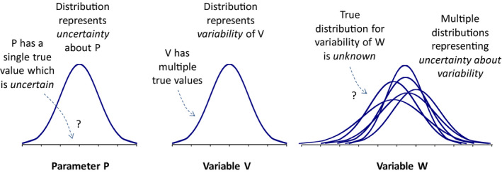
Illustration of the distinction between uncertainty and variability (left and central graphs), and that both can affect the same quantity (right hand graph)

Variability is a property of the real world, referring to real differences between the members of a population of real‐world entities. Although the term population is commonly used in relation to biological organisms (e.g. humans), the same concepts apply to populations of other types of entity (e.g. a class of related chemicals). Our knowledge of variability is generally incomplete, so there is uncertainty about variability (see graph on right side of Figure 1). Some types of variability, for example, the variation in human body weight, are much less uncertain than others, e.g. the variation of chemical concentrations in a type of food for which few measurements are available. When dealing with variability in scientific assessment, it is important to define clearly the population involved, and identify any relevant subpopulations. If the population, or individual values changes over time, it is necessary also to specify the time period of interest.

Although distinct, variability and uncertainty are also related, because some types of uncertainty are caused by variability. Variability in a population causes uncertainty about parameters such as the mean when they are estimated by measuring samples from that population (sampling uncertainty). The more variability there is in the population, the larger the sample that is needed to measure it with a given degree of precision. Imprecision is a form of measurement uncertainty, due to variability in repeated measurements of the same quantity. Uncertainty caused by variability is sometimes referred to as ‘aleatory’ uncertainty and distinguished from ‘epistemic’ uncertainty, which refers to other types of limitations in knowledge (e.g. Vose, 2008).

How variability and uncertainty for each component of an assessment should be treated depends on whether the assessment question refers to the population or to a particular member of that population, how each component of the assessment contributes to that, and how those contributions are represented in the assessment model. Many assessment questions refer to populations, e.g. what proportion of a population will experience a given level of exposure. Whether it is appropriate to quantify variability in a particular input depends on the question to be addressed. For example, variability in chemical concentrations needs to be quantified in assessments of acute exposure to chemicals, but mean concentrations are generally used when assessing long‐term exposure. An important example of a risk assessment component relating to a particular instance of a variable quantity is provided by the default assessment factors used in chemical risk assessment, as discussed in Annex B.16. The actual difference between animals and humans will vary between chemicals, and the extent of this variation is uncertain, so a default assessment factor needs to address both the variability and the uncertainty (as can be seen from the right graph of Figure 1). In an assessment for a single chemical, the variability should be treated as part of the uncertainty, whereas in an assessment of cumulative risk for multiple chemicals, the variability and uncertainty should be separated. Care is needed to determine when variability and uncertainty should be separated and when they should be combined, as inappropriate treatment may give misleading results.

5.4. Dependencies

Variables are often interdependent. In some cases, this is explicitly represented by models used in scientific assessment, e.g. dose–response models. But it can also apply to other variables: for example, body weight tends to be positively correlated with height and both are correlated with age. It is important to take account of dependencies between variables in assessment, because they can have a large effect on the result. This means that different combinations of values must be considered in proportion to their expected frequency, taking account of any dependencies, and excluding unrealistic or impossible combinations.

Sources of uncertainty can also be interdependent. This happens when learning more about one question or quantity in an assessment would alter the assessor's uncertainty about another question or quantity. For example, given two previously untested chemicals with similar structures, obtaining information about the toxicity of one of them might alter one's expectation about the toxicity of the other. Another example, which may be surprising, is that while it is well known that the means and variances of repeated samples from a normal distribution vary independently, the uncertainties of the population mean and variance for a normal distribution are interdependent, when estimated from a measured sample. This is because, if one discovered that the population mean was a long way from the sample mean, this would change the uncertainty of the variance, because high variances would become more likely. Where learning more about one source of uncertainty would not alter uncertainty about another and vice versa, they may be treated as independent; for example, information on the toxicity of one chemical may not alter one's expectation about the toxicity of other chemicals if they have very different structures.

Dependencies between sources of uncertainty can greatly alter the overall uncertainty, so it is important to identify them and take them into account. This is true not only when using distributions to take account of uncertainty. For example, in a deterministic assessment using conservative assumptions, it is important to consider dependencies between the assumptions when assessing the overall conservatism of the assessment (Section 11.6.3). It is very difficult to make reliable expert judgements about the effect of dependencies, whether for variability or uncertainty, and it is therefore preferable to assess them by probabilistic calculations than by expert judgement when possible (see Section 11.4.6). A simpler alternative is to use probability bounds methods, which do not require information or assumptions about dependencies (see Section 11.4.5).

Dependencies are not limited to assessments using quantitative methods. In assessments using qualitative methods, the assessors should also consider whether learning more about each element of the assessment would affect their uncertainty about other elements, and take this into account when evaluating the uncertainty of the assessment conclusions. For example, if ordinal scales are used to assess the uncertainty of different assessment inputs, it is important to consider the potential dependencies between those sources of uncertainty when assessing the uncertainty of the assessment as a whole. Again, this is difficult to do by expert judgement, and may be a reason to reformulate the assessment and/or uncertainty analysis in quantitative terms.

5.5. Models and model uncertainty

All scientific assessments involve some form of model, which may be qualitative or quantitative, and most assessments are based on specialised models relevant to the type of assessment. Many assessments combine models of different kinds.

Examples of types of model used by EFSA:

• Conceptual models representing fundamental scientific understanding of physical, chemical and biological processes and their interactions in organisms, environment and ecology.

• Models that do not estimate real observable quantities, but give structure to assessments and are useful for decision‐making. For example, hazard/exposure ratios in human and environmental risk assessment.

• Deterministic and probabilistic models of specific processes relevant to assessments. For example, chemical kinetics and dynamics, exposure, environmental fate, introduction and spread of species, agricultural practices, microbial contamination, cumulative effects of multiple stressors.

• Individual‐based probabilistic models. For example, individual based dietary exposure modelling, individual animals in the landscape.

• Statistical models. For example, standard statistical models of experimental measurements and sampling processes, regression and dose–response models, models of absorption/excretion of nutrients, and models of interchemical, interspecies and intraspecies variability of toxicity.

• Logic models: models expressing a yes/no conclusion as a logical deduction from the answers to a series of yes/no questions. The logic is represented using logical operators such as ‘AND’, ‘OR’ and ‘NOT’, e.g. if a AND b then c.

Types of uncertainties affecting the structure and inputs of models are discussed in Section 8.1. If uncertainties affecting inputs to quantitative models (including logic models) are quantified, they can be ‘propagated’ through the models to calculate the impact of those uncertainties on the model outputs.

Some types of uncertainty about model structure can be quantified statistically, e.g. by model averaging (Section 11.5.2). Other types of uncertainty about model structure must be assessed by expert judgement, and taken into account when characterising overall uncertainty (see Section 14). As is commonly said, all models are wrong but some are useful (Box, 1976). Therefore, judgements about model uncertainties should be expressed not as a probability that the model is correct, but as probability distributions or probability bounds for the difference between the model output and the real quantity it is intended to represent. While this is challenging for assessors, it should be possible because the decision to use a model already implies a judgement that the output will be reliable enough to provide a justifiable basis for scientific advice; if the assessors cannot make that judgement explicit then it is difficult to justify using the model.

All models are simplified abstractions of the real world. Nevertheless, some models directly address the scenario and question or quantity of interest to decision‐makers, for example, it is possible to model the proportion of people experiencing a specified effect in the EU population (IPCS, 2014). In other cases, to simplify the assessment, assessors develop models addressing simplified scenarios and/or surrogate questions or quantities. For example, they might assess the same effect only for a subset of EU countries, or (commonly) the proportion of people exceeding a specified exposure (e.g. a Health‐Based Guidance Value) rather than the proportion who experience effects. Ideally, extrapolation from the output of such a simplified model to the scenario and question or quantity of interest should be considered as a model uncertainty, and included in the characterisation of overall uncertainty (Section 14). However, this is not necessary if the decision‐makers and assessors agree that the model output can be used as the basis for decision‐making without such extrapolation. In effect, they have then agreed, or are willing to assume, that the difference between the model output and the scenario and question or quantity of interest will be too small to impact decision‐making. When a simplified model is used repeatedly for different assessments, the assumed extrapolation should be tested through an appropriate analysis: this is the reason for ‘calibration’ of standardised assessment procedures, which are a type of simplified model and common in many areas of EFSA's work (see Section 7.1.3).

5.6. Evidence, agreement, confidence and weight of evidence

Evidence, weight of evidence, agreement (e.g. between studies or between experts) and confidence are all concepts that are related to uncertainty. Increasing the amount, quality, consistency and relevance of evidence or the degree of agreement between experts tends to increase confidence and decrease uncertainty. Therefore, scales for evidence, agreement, etc. are sometimes used as measures of uncertainty. However, the relationship between these concepts is complex and variable. For example, obtaining more evidence or consulting more experts may reveal new issues that were previously not considered, and if so confidence decreases and uncertainty increases. As another example, two experimental studies may provide the same amount and quality of evidence for the same measurement, but differing confidence intervals. Furthermore, measures of evidence and agreement do not, on their own, provide information on the range and probability of possible answers or values, which is what matters for decision‐making (Section 3.1). Therefore, they are insufficient and may be misleading if used alone as measures of uncertainty. This is why EFSA Scientific Committee (2017a) recommends expressing the conclusions of weight of evidence assessment in terms of the relative support for possible answers to a question.

Nevertheless, because the amount, quality, consistency and relevance of evidence and the degree of agreement are related to the degree of uncertainty, consideration of evidence and agreement is useful as part of the process for assessing weight of evidence (EFSA Scientific Committee, 2017a,b) and in uncertainty analysis. Expressing evidence and agreement on defined qualitative scales can be helpful in structuring the assessment, facilitating discussion between experts and increasing consistency in the expression of their judgements (Section 10). Such scales also provide a summary of evidence and agreement that may be helpful to assessors when they are making judgements about the range and probability of possible answers or values for a question or quantity. An example of this is provided by Mastrandrea et al. (2010), who use categorical scales for evidence and agreement to inform judgements about the level of confidence in a conclusion and (when confidence is high) its probability.

The term ‘confidence’ is used in different ways, both quantitative and qualitative. The familiar quantitative use is in statistical analysis, where a confidence interval for a statistical estimate (e.g. a mean) provides a measure of its uncertainty. The level of confidence for the interval is specified as a (frequentist) probability, and quantifies only that part of uncertainty that is reflected in the sampling scheme and the variability of the data being analysed (see Section 5.10). The use of confidence intervals in uncertainty analysis is discussed in Section 5.10 and 11.2.1.

The term ‘confidence’ has also been used as a qualitative measure of trust in a conclusion, expressed on a qualitative scale. Such scales are subject to the same limitations as other qualitative expressions of uncertainty, but again may be useful as an aid to assessors when making more quantitative judgements. For example, Mastrandrea et al. (2010) propose an ordinal scale for confidence with five levels (‘very low’, ‘low’, ‘medium’, ‘high’ and ‘very high’). They emphasise that this is different from statistical confidence, and describe it as synthesising assessors’ judgements about the validity of findings as determined through evaluation of evidence and agreement (see Section 11.3.3 and Annex B.3 for further aspects of their approach, and Section 10.2 and Annex B.2 for more on ordinal scales in general).

The term ‘weight of evidence’ is often used in situations where there are multiple studies on the same topic, or multiple lines of evidence for the same question, which may be of differing relevance and reliability or show contrasting results. A weight of evidence approach involves weighing the different studies or lines of evidence against each other, taking account of their reliability and their relevance to the question being assessed, and assessing the balance of evidence for or against different conclusions. Methods for weight of evidence assessment are the subject of a separate guidance document (EFSA Scientific Committee, 2017a,b). Weight of evidence assessment and uncertainty analysis are closely related: the former characterises part of the uncertainty affecting the conclusion but not all. In particular, it does not include uncertainties affecting the selection of evidence to include, and the choice of methods for evaluating and integrating the evidence, which must therefore be taken into account by uncertainty analysis (see Sections 2.6 and 4.5 in EFSA Scientific Committee, 2017a,b).

5.7. Influence, sensitivity and prioritisation of uncertainties

Influence and sensitivity are terms used to refer to the extent to which plausible changes in the overall structure, parameters and assumptions used in an assessment produce a change in the results. Analysis of sensitivity and influence has several uses in uncertainty analysis. It can be used to evaluate the overall robustness of the conclusion with respect to choices made in the assessment (including methods used to assess the uncertainty). As such, it can help to inform judgements about the contribution of these choices to uncertainty of the question or quantity of interest. It also plays an important role in prioritising the most important uncertainties for additional analysis or data collection. In various fields, these terms are given specific technical meanings which however are not universal. In this document, they are used with specific meanings described below.

In general, and specifically in the context of uncertainty analysis (Saltelli et al., 2008), the term sensitivity analysis is used in the context of a quantitative model. There it refers to the quantitative measurement of the impact, on the output of the model, of changes to the values of inputs to the model. For consistency with this usage, in this document, the concept of sensitivity is restricted to the quantitative influence of uncertainty about inputs on uncertainty about the output of a mathematical model. The results of a sensitivity analysis can quantify the relative contribution of different input uncertainties to the uncertainty of the assessment output.

The term ‘influence’ is used in the Guidance in a broader sense and for all types of assessment, not just mathematical models. It refers to any possible change in the assessment output resulting not just from uncertainties about inputs to the assessment but also from uncertainties about choices made in the assessment. The latter might include the structure to use for the assessment, structure of models, choice of factors to include in models, etc. Quantitative assessment of influence is more complex than assessment of sensitivity and cannot be carried out using only the methods described in the annex on Sensitivity Analysis (B.17). It often requires replicating the assessment with different assumptions, models, etc. (e.g. what‐if calculations or scenario analysis). If time and resource constraints do not permit such replication, this needs to be taken into account in the characterisation of overall uncertainty (see Section 14). Influence can also be assessed qualitatively, e.g. using ordinal scales to express qualitative judgements about the relative influence of different uncertainties on the assessment output.

Prioritisation of uncertainties is useful both during an assessment and at its end. Early in the assessment, after identifying sources of uncertainty and before commencing quantitative analysis, qualitative assessment of influence can help assessors to decide which uncertainties to analyse in detail and which will be evaluated collectively later in the analysis, when characterising overall uncertainty. The initial prioritisation of sources of uncertainty is necessarily an approximate exercise, but this is sufficient because the contribution of the sources of uncertainty that are prioritised will be considered again when characterising overall uncertainty (Section 14). They can then be selected for further evaluation in a subsequent iteration of the uncertainty analysis if needed. During the course of the analysis, either influence or sensitivity analysis may be used to target the use of more refined and rigorous methods on the most important uncertainties. A specific example of this is the combination of ‘minimal assessment’ and sensitivity analysis, which was described by EFSA (2014a,b) as an approach to prioritising uncertainties for formal EKE. Sensitivity and influence analysis have therefore a key role to play in the iterative refinement of an assessment. Finally, at the end of the assessment, sensitivity and influence analysis can provide the basis for recommendations on priorities for future monitoring, data collection or research.

5.8. Conservative assessments

Many areas of EFSA's work use deterministic assessments that are designed to be ‘conservative’. The meaning of being conservative is discussed in detail by IPCS (2014) in the context of chemical hazard characterisation, but the same principles apply to all types of conservative assessment.

IPCS (2014) state that the word ‘conservative’ is generally used in the sense of being ‘on the safe side’ and can be applied either to the choice of protection goals, and hence to the question for assessment, or to dealing with uncertainty in the assessment itself.

The question for assessment might be framed in a conservative way (e.g. focussing on conservative scenario or subpopulation or on a mild level of effect) for various reasons. A common reason is to simplify the assessment of a complex set of conditions by focussing it on a conservative subset, which is protective of the rest. Another possible reason would be to deal with uncertainty in risk management considerations influencing the setting of protection goals, which causes uncertainty in the framing of the assessment question.

When used to deal with uncertainty in the scientific assessment, the term ‘conservative’ can refer to two different but related concepts. It can be used to mean that there is a high probability that the assessment result is ‘on the safe side’, i.e. more adverse than the real answer or value. On the other hand, ‘conservative’ can also be used to mean it is possible that a real value is much less adverse than the assessors’ estimate. IPCS (2014) refer to these two concepts of conservatism as ‘coverage’ and ‘degree of uncertainty’, respectively. When applied to a conservative estimate of a quantity, coverage refers to the probability that the real value is less adverse and degree of uncertainty to the amount by which the real value might be less adverse, measured by the width of a suitable credible interval for it. The concepts are related, but distinct: point estimates for two quantities might have the same coverage, but very different degrees of uncertainty (see Figure 2). IPCS (2014) illustrates these concepts in relation to the estimation of a point of departure in chemical hazard characterisation, which is intended to provide a conservative estimate of the dose of chemical required to cause an adverse effect. IPCS (2014) also explains why both concepts are of interest for decision‐making: coverage expresses the probability of less adverse values, while degree of uncertainty indicates how much the estimate might be reduced by further analysis or investigation. If coverage is low, decision‐makers may consider the assessment to be insufficiently conservative. On the other hand, if the real value could be much less adverse (high degree of uncertainty), decision‐makers may consider the assessment to be over‐conservative.

Figure 2.

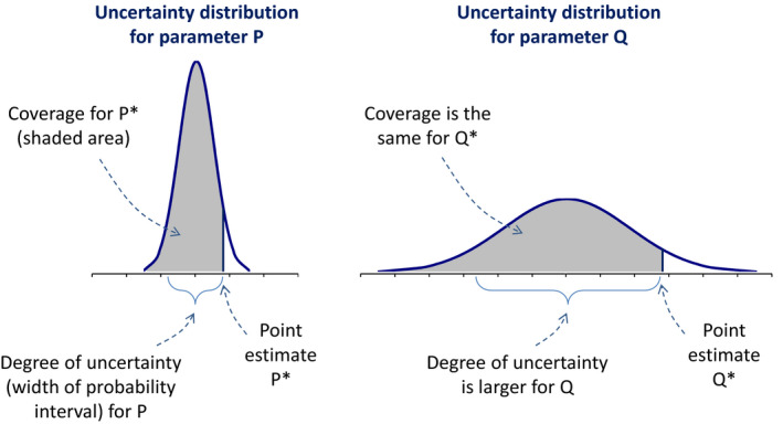
Illustration of the distinction between ‘coverage’ and ‘degree of uncertainty’ as measures of degree of conservatism. The distributions show uncertainty for two parameters P and Q. The point estimates P* and Q* have equal coverage (probability of lower values) but different degrees of uncertainty

Describing a quantitative estimate as conservative requires or implies three elements: specification of the quantity of interest and the management objective or protection goal, e.g. what is the maximum acceptable value; what maximum probability of more adverse values is acceptable; and derivation of a point estimate such that real values more adverse than the acceptable maximum are expected with no more than the specified probability. The first two elements involve risk management judgements that should ultimately be made by decision‐makers, although they may need help from assessors to interpret information on adversity, while the third element requires assessment of the uncertainty of the quantity of interest and should be done by assessors. Asserting that an estimate is conservative without specifying the target quantity and probability conflates the roles of decision‐makers and assessors and is not transparent, because it implies acceptance of some probability of more adverse values without making clear either what is meant by adverse or what the probability is. Therefore, if the decision‐makers wish to receive a single conservative estimate, they should specify the quantity of interest, an acceptable limit for the value, and the maximum acceptable probability of breaching that limit when setting the ToR for the assessment, as has been proposed by IPCS (2014) for chemical hazard characterisation. Alternatively, the assessors could provide a range of estimates for different levels of adversity and probability, so that the final choice remains with the decision‐maker.

Similar considerations apply to qualitative assessments and assessments of categorical questions (e.g. yes/no questions), which may also be designed to be ‘conservative’. Uncertainty about what category or qualitative descriptor should apply may be dealt with by assigning a more adverse category or descriptor. As for quantitative assessments, asserting that a categorical assessment is conservative implies both a scientific judgement (what is the probability that the adverse category actually applies) and a value judgement (what probability would justify assigning the adverse category for management purposes). If the decision‐maker wishes the assessor to assign a single category, they should specify the level of probability required. Otherwise, the assessor should report their assessment of the probability of each category, and leave value judgements to the decision‐maker.

Deterministic assessments with conservative assumptions are simple and quick to use and provide an important tool for EFSA, provided that the required level of conservatism is defined and that the assessment procedure has been demonstrated to provide it. These requirements are discussed in more detail for quantitative assessments in Section 11.6.3 and Annex B.16. If the same set of conservative assumptions will be used repeatedly in different assessments, as is common in standardised procedures, it becomes especially important to calibrate the degree of conservatism they provide, as described in Section 7.1.3.

It is not necessary for the assessor to express estimates or their probability as precise values, nor for the decision‐maker to express the required level of conservatism precisely. For example, if the purpose is to be conservative, then it may be sufficient to give a bound for the estimate and/or a lower bound for probability, providing information on coverage but not degree of uncertainty (as defined above). However, decision‐makers may also wish to place an upper limit on the degree of conservatism, to avoid disproportionate precaution in decision‐making. This requires information on degree of uncertainty as well as coverage, although again bounded values might be sufficient for this. Approximate probabilities are discussed further in Section 5.10 (below) and probability bounds (approximate probabilities for ranges) in Section 5.11 (below). If a probability bound is elicited for each input to a deterministic assessment, probability bounds analysis can be used to calculate a probability bound for the assessment output. This is much simpler than a fully probabilistic calculation and much more rigorous than a direct expert judgement about the conservatism of the assessment as a whole. It is therefore recommended that consideration be given to increased use of probability bounds analysis in case‐specific assessments and when calibrating standardised procedures.

5.9. Expert judgement

Assessing uncertainty relies on expert judgement, which includes an element of subjectivity because different people have different knowledge and experience and therefore different uncertainty (Section 5.2). Indeed, this is true of science in general. Choosing a model or chain of reasoning for the assessment involves expert judgements. The choice of assessment scenarios requires judgement, as does the decision to use a default assessment factor or the choice of a non‐standard factor specific to the case in hand. In probabilistic assessments, the choice of distributions and assumptions about their dependence or independence are subjective. Even when working with ‘hard’ data, assessing the reliability and relevance (internal and external validity) of those data is subjective. Even ideal data are rarely truly representative, so implicit or explicit judgements about extrapolation are needed (e.g. from one country to another or the EU as a whole, between age groups or sexes, and from the past to the present or future). And when using a confidence interval, or other representation of uncertainty deriving from statistical analysis of data, assessors must consider, explicitly or implicitly, if it accounts for all uncertainties that affect its use in the assessment, or whether some adjustment is required (see Section 11.2.1). When these various types of choices are made, the assessors implicitly consider the range of alternatives for each choice and how well they represent what is known about the problem in hand: in other words, their uncertainty. Thus, the subjective judgement of uncertainty is fundamental, ubiquitous and unavoidable in scientific assessment.

The Scientific Committee emphasises that expert judgement is not guesswork or a substitute for evidence. On the contrary, expert judgement must always be based on reasoned consideration of relevant evidence and expertise, which must be documented transparently, and experts should be knowledgeable or skilled in the topics on which they advise.

Well‐reasoned judgements are an essential ingredient of good science. However, judgements are made by psychological processes that are vulnerable to various cognitive biases (Kahneman et al., 1982). These include anchoring and adjustment, availability, range‐frequency compromise, representativeness and others. Additional psychological and social factors operate when experts work in groups, such as disproportionate influence of some individuals within the group and a tendency for over‐confidence in consensus judgements. An overview of these issues and references to more detailed literature are provided by EFSA (2014a). In addition, the judgements of individuals could be influenced, intentionally or unintentionally, by any personal interests they have in the issue under assessment: to guard against this, EFSA has stringent procedures which require experts to declare potential interests and exclude them from discussion of topics where conflicts of interest are identified.

Formal approaches for ‘expert knowledge elicitation’ have been developed to counter the psychological biases affecting expert judgement and to manage the sharing and aggregation of judgements between experts (see Section 11.3). EFSA has published guidance on the application of these approaches to eliciting judgements for quantitative parameters (EFSA, 2014a). This includes guidance on the selection and number of experts, and is designed to enable participation of individuals who would not normally be members of EFSA Panels and Working Groups when appropriate to the needs of the question, including people with practical knowledge of relevant processes such as food production. Some approaches to addressing uncertainty favour extending participation in the assessment beyond scientific experts, to include stakeholders and the public, especially when the limits to knowledge are severe (e.g. Stirling, 2010; IRGC 2012). This is discussed further in Section 5.12.

EFSA (2014a) describes procedures for formal EKE, which require significant time and resources. It is recognised that more streamlined approaches will be needed in many cases. Furthermore, in some parts of EFSA's work, legal deadlines and resource limitations require that some judgements will be made by small groups or even a single expert. Modified EKE procedures to deal with these issues are described in Section 11.3.1. In all cases, the basic principles for eliciting expert judgements should be respected.

Experts often have differing views on the same question. This is natural, because they have different experience, knowledge and expertise, and is beneficial because it broadens the evidence base for assessment. Where a wide range of scientific opinion exists, the experts should be selected to represent it. Interaction between experts may produce a degree of consensus, as information is shared and interpretations are discussed. However, consensus should not imply compromise (EFSA, 2014a): where differences of opinion remain between experts this is part of scientific uncertainty and should be reflected in the assessment report, either within the uncertainty analysis or, when appropriate, through EFSA's procedure for minority opinions, so it can be taken into account by decision‐makers.

The Scientific Committee stresses that where suitable data provide most of the available information on an issue and are amenable to statistical analysis, this should be used in preference to relying solely on expert judgement. However, as noted above, most data are subject to some limitations in reliability or relevance, and further uncertainties arise in the choice of statistical model; the greater these limitations and uncertainties, the more the results of statistical analysis will need to be interpreted and/or augmented by expert judgement (Section 11.2.1).

The Scientific Committee recognises that some assessors have concerns about quantifying uncertainty using expert judgement, for various reasons. Those concerns have been considered and addressed in developing this document and the accompanying Guidance, as summarised in Section 4.2 (Box 2). When making probability judgements in EFSA assessments, suitable training should be provided to the experts involved (EFSA, 2014a), and any concerns they may have should be discussed.

It has been demonstrated that people often perform poorly at judging combinations of probabilities (Gigerenzer, 2002). This implies they may perform poorly at judging how multiple sources of uncertainty in an assessment combine. Therefore, the Guidance recommends that uncertainties should be combined by calculation when possible, even if the calculation is very simple (e.g. a series of what‐if calculations with alternative assumptions, or approximate probability calculations (see Section 11.6)), to help inform judgements about the overall uncertainty from the identified sources. When doing this, assessors should take account of the additional uncertainties associated with choosing the calculation model, and avoid using combinations of inputs that could not occur together in reality. If sources of uncertainty are combined by expert judgement, then the assessors should try to take account of the added uncertainty that this introduces (e.g. widen their range or distribution for the overall uncertainty until they judge that it represents the range of results they consider plausible).

5.10. Probability

When dealing with uncertainty, decision‐makers need to know the range and probability of possible answers for questions or quantities they submit for scientific assessment (Section 3.1). There are two major views about the scope of probability as a measure for quantifying uncertainty. One, sometimes known as the frequentist view, considers that the use of probability should be restricted to uncertainties caused by variability and should not be applied to uncertainties caused by limitations in knowledge. As a result, it offers no solution for characterising the many other types of uncertainty that are not caused by variability (e.g. data quality, extrapolation), which are frequently important in EFSA assessments.

The other, subjectivist (Bayesian), view asserts that a probability is a direct personal statement of uncertainty and that the uncertainty of any well‐defined question or quantity (see Section 5.1) can be quantified using probability. It can therefore represent uncertainties caused by limitations in knowledge as well as those caused by variability.

A key advantage of subjective probability as a quantitative measure of uncertainty is that there are ways to enhance comparability when probabilities are expressed by different individuals. Informally, an individual can compare any particular uncertainty to situations where there is a shared understanding of what different levels of probability mean: tossing a fair coin, rolling fair dice, etc. Formally, an operational definition of subjective probability was developed by de Finetti (1937) and Savage (1954), in part to ensure comparability. An important consequence of this is that subjective probabilities or approximate probabilities can be given for any well‐defined quantity or categorical question (de Finetti, 1937; Walley, 1991). In everyday language, it is possible to give a subjective probability for anything that one could bet on, that is, if it would be possible in principle to determine without ambiguity whether the bet was won or lost. For example, one can bet on the final score of a sports event, but not on whether it will be a ‘good game’ because different people will interpret that in different ways.

The operational definition of subjective probability leads to a second key advantage. It shows that the extensive mathematical and computational tools of probability can legitimately be applied to subjective probabilities. In particular, those tools aid expression of judgements about combinations of sources of uncertainty (e.g. in different parts of an uncertainty analysis) which the human mind would otherwise find difficult. In other words, it can help the assessors make more rational judgements about questions such as: if I can express my uncertainty about hazard and exposure, then what should my uncertainty be about risk? For these reasons, the Guidance encourages the use of subjective probability to express uncertainty, except when assessors find it too difficult to quantify uncertainty (see Section 5.12).

The subjectivist interpretation of probability does not exclude the frequentist interpretation. However, it is necessary to reinterpret a frequentist probability as a subjective probability before it can properly be combined with subjective probabilities in calculations involving multiple sources of uncertainty. This has implications for how probabilities based on statistical analysis of data are combined with probabilities derived directly from expert judgement. If the statistical analysis is Bayesian, the result is already a subjective probability. However, if the analysis results in a confidence interval, reinterpretation would be needed, since the associated confidence level is a frequentist probability. For more details of how such reinterpretation works, and when it is appropriate, see the discussion of confidence intervals in Section 11.2.1. Any probability arising from a statistical analysis is likely to be subject to additional uncertainties, not addressed by the analysis, which need to be taken into account and which must be addressed by expert judgement.

It is not necessary to express probabilities fully or precisely, and in practice they will always be approximate to some degree (assessors will not specify them to an infinite number of decimal places). An approximate probability, specified as a range for the probability, may be easier for assessors to provide, and may be more acceptable to those who consider that giving an exact probability exaggerates the precision of subjective judgement. For example, it may be simpler for assessors to judge that an adverse consequence has less than a given probability, rather than giving a specific probability, and if that probability is low enough it may be sufficient for decision‐making. This type of judgement is implicit in many conservative assessment procedures: they do not provide a precise probability, but they indicate at least a sufficient probability of avoiding adverse consequences. Approximate probabilities can also be used by assessors to express their confidence in their probability judgements: for example, a wider range of probability might be given when the evidence is weaker, or when the assessors’ expertise is less directly relevant to the question (this would be acceptable to proponents of imprecise probability such as Walley (1991), though not to traditional subjectivist Bayesians who use only precise probabilities). Thus, assessors might give an approximate probability either because it is simple and sufficient, or because they are unable to provide a more complete probability statement. Although the reasons for specifying approximate probabilities may vary, the mathematics for computing with them are the same.

5.11. Overall uncertainty

The recommendation to express uncertainty quantitatively applies specifically to overall uncertainty (Section 4.2). It is important to be clear what is meant by the term overall uncertainty, when used in this document and the accompanying Guidance. It refers to the assessors’ uncertainty about the assessment conclusion at the time of reporting, taking account of the combined effect of all sources of uncertainty identified by the assessors as being relevant to the assessment.

Assessors should try to express the overall impact of all identified uncertainties in quantitative terms. Where this is not possible, they should document qualitatively those uncertainties they were unable to include in the quantitative expression. Taken together, the quantitative and (if any) qualitative expressions constitute the assessors’ characterisation of their overall uncertainty.

In some areas of EFSA's work, decision‐makers or legislation may require that conclusions be reported qualitatively, or require unqualified positive or negative conclusions. This should be dealt with as described in Section 3.5. However, quantitative evaluation of overall uncertainty is still needed in such cases, to determine what conclusion is justified, even though the conclusion itself will be in qualitative form (see Section 3.5). The exception to this is in standardised assessments where no non‐standard uncertainties are identified.

It is important to note that overall uncertainty cannot and does not include any information about unknown unknowns, i.e. uncertainties not known to the assessors. Since these are unknown, they cannot be either quantified or described. Furthermore, it must be remembered that the characterisation of uncertainty is conditional on the assessors who provide it, and on the evidence, time and resources available to them (Section 5.2). These things should be understood by decision‐makers and taken into account by them when interpreting and using the assessment conclusions (see Section 5.13).

5.12. Unquantified uncertainties

The term unquantified uncertainties is used in this document and the accompanying Guidance to refer to uncertainties which the assessors have identified as relevant to their assessment, but are unable to include in their quantitative expression of overall uncertainty. This section discusses different perspectives on the limits to what can be quantified, including what makes an uncertainty literally unquantifiable, and what can be done about those uncertainties that assessors are unable to quantify.

Assessors should seek to ensure that all questions or quantities considered in their assessments are well‐defined. If they are unable to achieve this, then the uncertainty of those questions or quantities is literally unquantifiable (Section 5.10). However, even when a question or quantity is well‐defined, an assessor may sometimes be unable to quantify one or more uncertainties affecting it, if they cannot make any quantitative judgement of the magnitude of a source of uncertainty or its impact on the assessment. In such cases it is, for that assessor, not possible to quantify those uncertainties, with the evidence available to them at the time of the assessment. Sources of uncertainty that are not quantified for either reason (inability to define or inability to quantify) are sometimes referred to as ‘deep’ uncertainties and are most likely to arise in problems that are novel or complex (Stirling, 2010).

A number of authors including Stirling, especially in social science, economics and some in environmental science, give precedence to a concept of uncertainty based on the work of the economist Frank Knight (1921). They regard uncertainty as unquantifiable by definition and distinguish it from quantifiable incertitude, which they term ‘risk’. This tends to be linked to a frequentist view of probability, and to a view that uncertainty can only be quantified when all possibilities can be enumerated. However, as noted by Cooke (2015), Knight said ‘We can also employ the terms ‘objective’ and ‘subjective’ probability to designate the risk and uncertainty, respectively, as these expressions are already in general use with a signification akin to that proposed’. The Guidance uses subjective probability, for the reasons explained in Section 5.10. Subjective probability can be used to express any type of uncertainty, including that caused by variability, provided the question or quantity of interest is well defined. It does not require enumeration of all possibilities, only that the possibilities considered are well defined (e.g. the occurrence or non‐occurrence of a well‐defined consequence). However, the Scientific Committee acknowledges that assessors may not be able to quantify some sources of uncertainty, even when the questions or quantities of interest are well defined.

Stirling (2010) presents a matrix which defines 4 conditions of incertitude (risk, uncertainty, ambiguity and ignorance), relates them to the extent of understanding about possibilities and probabilities. In practice, these conditions relate to individual sources of uncertainty, rather than to the assessment as a whole. Some uncertainties are well defined, and some of those are quantifiable. Other uncertainties are poorly defined (ambiguous), and some relate to unidentified, unknown or novel possibilities (ignorance or ‘unknown unknowns’). Most assessments are affected by multiple sources of uncertainty, some of which can be assigned to one condition and some to others. For this reason, the Guidance emphasises the need to identify, within each assessment, which sources of uncertainty are quantified and which are not. It recommends seeking to include as many as possible of the identified sources of uncertainty in a quantitative expression of overall uncertainty, for the reasons explained in Section 4.2; in addition, trying to quantify sources of uncertainty is a practical way for assessors to identify which uncertainties they cannot quantify. Stirling's (2010) matrix indicates different methods for dealing with each of the 4 conditions of incertitude. Some of these methods involve participation of stakeholders or other parties, some include consideration of values as well as scientific considerations, and some are strategies for managing uncertainty and risk rather than assessing it. Other authors also recommend involving stakeholders in dealing with uncertain and ambiguous risks (e.g. IRGC, 2012). Such approaches are outside the remit of EFSA, which is restricted to scientific assessment, produced by a Scientific Committee and Panels constituted of independent scientific experts (with the option to hold public hearings). The role EFSA can serve is to identify scientific sources of uncertainty, quantify them where possible, identify and describe uncertainties it cannot quantify, and report these in a transparent way to those requesting the assessment. It is then for others to decide whether to submit the uncertainties to additional processes or consultation to assist decision‐making.

When assessors are unable to quantify some of the identified uncertainties affecting an assessment, it is essential that they describe them qualitatively and report this together with their quantitative expression of overall uncertainty, as the latter will then be conditional on assumptions made in the assessment regarding the sources of uncertainty that were not quantified. This has important implications for reporting and decision‐making, which are considered in Section 5.13.

5.13. Conditionality of assessments

Assessments are conditional on any sources of uncertainty that have not been included in the quantitative assessment of overall uncertainty. This is because the assessment will necessarily imply assumptions about those sources of uncertainty, and therefore, the output of the assessment is that which would apply if the assumptions were true.

It is important to recognise that all assessments are conditional to some extent. They are conditional on the current state of scientific knowledge, on that part of existing knowledge that is available to the assessors at the time of assessment, and on their judgements about the question under assessment (Section 5.2). Therefore, all assessments refer to what would apply if the assessors had identified all relevant sources of uncertainty, and if there were no ‘unknown unknowns’ affecting the question under assessment. These sources of conditionality are general, in the sense that they apply to all assessments.

In addition to this general conditionality, further, case‐specific conditionality is added when one or more of the identified sources of uncertainty in a particular assessment are not included in the quantitative expression of overall uncertainty. That quantitative expression then becomes conditional also on the assumptions made for those identified sources of uncertainty that remain unquantified. In effect, these assumptions define a scenario, on which the assessment is conditional. Since the assumptions relate to sources of uncertainty that the assessors could not quantify, they will be unable to say anything about the probability that the scenario will actually occur, although they may be able to say it is possible. An example of explicit reporting of the conditionality of an assessment is provided by EFSA's (2008) statement on melamine, summarised in Annex A.2, which reported that exposure estimates for a high exposure scenario exceeded the tolerable daily intake (TDI), but stated that it was unknown whether such a scenario may occur in Europe.

Conditionality has important implications for decision‐making, because it means the assessment conclusion is valid only if the assumptions on which it is conditional are valid, and provides no information about the probability those assumptions are valid, nor about what might happen if they are invalid. In such cases, therefore, assessors should consider whether it is justified to offer the conditional conclusion as scientific advice or, instead, report that the assessment is inconclusive. If they do report a conclusion, it is essential that decision‐makers are made aware of the assumptions on which it depends.

Decision‐makers should understand that all assessments are conditional on the current state of scientific knowledge, and do not take account of ‘unknown unknowns’, and take this into account in decision‐making (e.g. they might treat novel issues differently from those with a long history of scientific research). Similarly, they should understand that assessments are conditional on the experts who provide them, and the time and resources allocated for assessment, and take these into account (e.g. by giving more time and resource to assessments of more critical issues). However, they cannot be expected to identify for themselves which of the identified sources of uncertainty the assessors have not included in their quantitative assessment of overall uncertainty, nor what assumptions have been made about them.

Every assessment report must therefore include a list of those identified sources of uncertainty that the assessors have not included in their quantitative assessment of overall uncertainty. These sources of uncertainty will need to be described in detail, since the decision‐makers must decide how to deal with them, e.g. whether to ignore them, commission further research, or take precautionary action. These decisions will necessarily imply judgements about the potential magnitude of the unquantified uncertainties, which generally would be better made by assessors (if they are scientific uncertainties). This underlines the need for assessors to include them in their quantitative expression of overall uncertainty. If this is not possible, assessors should state the locations of the sources of unquantified uncertainty within the assessment, describe as far as possible the cause and nature of each one, explain why the assessors were unable to include it in the quantitative assessment and, most importantly, state what assumptions about each uncertainty have been made or implied in the assessment. In addition, they should identify any further analysis or research that might make it possible to quantify these sources of uncertainty, so that decision‐makers can consider whether to invest in it.

The assessor should communicate clearly to the decision‐maker – as was done in the 2008 melamine statement (see above) – that they are unable to say anything about the probability of assumptions about unquantified sources of uncertainty being true, or about how different the real consequences might be from what is indicated by the assessment. They must not use any language that implies a quantitative judgement about the probability of other conditions or their effect on the conclusion (e.g. ‘unlikely’, ‘negligible difference’). If the assessor feels able to use such language, this implies that they are in fact able to make a quantitative judgement. If so, they should express it quantitatively or use words with quantitative definitions (e.g. Table 3, Section 11.3.3) – for transparency, to avoid ambiguity, and to avoid the risk management connotations that verbal expressions often imply (Section 4.2).

Although assessors can provide only limited information about the sources of uncertainty they cannot quantify, it is still important information for decision‐makers. It makes clear what science can and cannot contribute to informing their decisions, and assists them in targeting further analysis or research. In some cases, the unquantified sources of uncertainty may relate to factors the decision‐makers can influence, e.g. uptake or enforcement of particular practices.

5.14. Types of assessment distinguished for uncertainty analysis

It is useful for later parts of this document to introduce some terms and concepts that will be used to distinguish different types of scientific assessment, which require different approaches to uncertainty analysis as outlined below and discussed in more detail in Section 7.1. Four main types of EFSA assessment are distinguished, described below. The boundaries between the four types are not sharply defined: for example, there are varying degrees of urgency. However, the purpose of the types is not to classify assessments, but to aid assessors in deciding what approach to take to uncertainty analysis, as set out in different sections of the accompanying Guidance. It is expected that most assessments will be readily assigned to one of the four types. In cases where more than one type could apply, assessors should consider directly which of the approaches in the Guidance is most suitable for the needs of their assessment. The four types are as follows:

• Standardised procedures with accepted provision for uncertainty. These include standardised elements to take account of uncertainty (e.g. assessment factors, default values, conservative assumptions), which are accepted by assessors and decision‐makers as appropriate and sufficient to address the sources of uncertainty affecting the class of assessments they are used in. Such procedures can be regarded as part of risk assessment policy in the sense of Codex (2016),5 and are commonly used in the assessment of regulated products. In many cases, these approaches have developed over time and are accepted as a matter of convention (see Section 7.1.2). In assessments using standardised procedures, a minimal uncertainty analysis may be sufficient to confirm that the standard provision is appropriate for the case in hand. This should include a check for any case‐specific uncertainties that are not adequately covered by the standardised procedure; if any are found, case‐specific assessment will be needed instead (see below).

• Case‐specific assessments. These are needed in the following situations:

  • 1—  there is no standardised procedure for the type of assessment in hand;
  • 2—  there is a standardised procedure, but there are case‐specific sources of uncertainty that are not included, or not adequately covered, by the standardised procedure;
  • 3—  a standardised procedure has identified a potential concern, which is being addressed by a refined assessment involving data, methods or assumptions that are not covered by the standardised procedure;
  • 4—  assessments where elements of a standardised procedure are being used but other aspects are case‐specific.

• In such assessments, a case‐specific uncertainty analysis is needed, following the general approach outlined in Section 7.1.1 of this document.

• Review of an existing standardised procedure or development of a new one, for example, when reviewing existing guidance documents or developing new ones. This will require a case‐specific uncertainty analysis of the procedure to support the acceptance of a new procedure or continued acceptance of an established one. This will ensure that it provides an appropriate level of coverage for the sources of uncertainty that will be encountered in the assessments for which it is used (see Section 7.1.3).

• Urgent assessments, for which there are exceptional limitations on time and resources. For such assessments, a minimal uncertainty analysis is still essential but can be scaled to fit within the time and resources available (see Section 7.1.4).

In some areas of EFSA's work, the result of a standardised assessment may indicate the need for a ‘refined’ or ‘higher tier’ assessment in which one or more standardised elements are replaced by case‐specific approaches. In principle, the assessment becomes case‐specific at this point for the purpose of uncertainty analysis, although it may be possible to treat it as a standardised assessment with some non‐standard uncertainties; both options are included in the accompanying Guidance.

Assessors often distinguish between quantitative and qualitative assessments. This sometimes refers to the form in which the conclusion of the assessment is expressed: either as an estimate of a quantity of interest (quantitative), or as a verbal response to a question of interest (qualitative). In other cases, an assessment may be described as qualitative because the methods used to reach the conclusion do not involve calculations; e.g. when the conclusions are based on a combination of literature review and narrative reasoning. In all cases, the conclusions of qualitative assessments must be expressed in a well‐defined manner, for the reasons explained in Section 5.1. Any well‐defined qualitative conclusion can therefore be considered as an answer to a yes/no question; this is important for uncertainty analysis, because uncertainty about a well‐defined yes/no question can be expressed quantitatively, using probability. This is very important for uncertainty analysis, because it means uncertainty can be quantified using probability for qualitative assessments as well as for quantitative ones. In general, therefore, the fact that an assessment uses qualitative methods or its conclusion is expressed in qualitative terms does not imply that the uncertainty analysis must be qualitative: on the contrary, assessors should try to express uncertainty quantitatively, for the reasons discussed in Section 4.2. Qualitative methods of expressing uncertainty also have important uses in uncertainty analysis, however (Section 4.3).

6. Main elements of uncertainty analysis

The main elements of uncertainty analysis are listed in Box 3. As indicated in Box 2, some of the elements are required in every assessment, while others are needed in some assessments but not others. What is needed depends in part on the general type of the assessment (standardised assessment, case‐specific assessment, development or review of a standardised procedure, urgent assessment) as discussed in Sections 5.14 and 7.1, and partly on the specific needs of the individual assessment, which need to be decided by assessors. Some elements are only needed when the uncertainty analysis is divided into parts, the motivation and approaches for which are discussed in Section 7.2. Furthermore, there are multiple options and methods available for implementing each element, the choice of which also depends on the needs of each assessment. Assessors therefore need first to identify which type of assessment they have in hand and what its specific needs are, decide which elements of uncertainty analysis are required and, within each element, choose which methods or options to apply. Detailed advice on these choices is provided in the form of flow charts in the accompanying Guidance (EFSA Scientific Committee, 2018). By following the flow charts, assessors should be able to construct an appropriate uncertainty analysis for each assessment, comprising the relevant elements and appropriate options and methods. Some of the major factors considered when developing the flow charts are discussed in Section 7.

Box 3: Main elements of uncertainty analysis. Some assessments require only some elements, and each element can be implemented in various ways with various methods. Flow charts in the accompanying Guidance (EFSA Scientific Committee, 2018) provide guidance on the choice of elements, options and methods for different types of assessment.

Identifying uncertainties affecting the assessment. This is necessary in every assessment, and should be done in a structured way to minimise the chance of overlooking relevant uncertainties, as described in Section 8. In assessments that follow standardised procedures, it is only necessary to identify non‐standard uncertainties (examples of these are given in Section 7.1.2).

Prioritising uncertainties within the assessment plays an important role in the planning the uncertainty analysis, enabling the assessor to focus detailed analysis on the most important uncertainties and address others collectively when evaluating overall uncertainty. Often prioritisation will be done by expert judgement during the planning process, but in more complex assessments it may be done explicitly, using influence or sensitivity analysis (see Section 5.7 and 12).

Dividing the uncertainty analysis into parts (when appropriate). In some assessments, it may be sufficient to characterise overall uncertainty for the whole assessment directly, by expert judgement. In other cases, it may be preferable to evaluate uncertainty for some or all parts of the assessment separately and then combine them, either by calculation or expert judgement. These options are discussed in more detail in Section 7.2.

Ensuring the questions or quantities of interest are well‐defined. This is necessary in every assessment, for reasons discussed in Section 5.1. Some assessments follow standardised procedures, within which the questions and/or quantities of interest should be predefined. In other assessments, the assessors will need to identify and define the questions and/or quantities of interest case by case, as described in Section 5.1.

Characterising uncertainty for parts of the uncertainty analysis. This is needed for assessments where the assessors choose to divide the uncertainty analysis into parts, but may only be done for some of the parts, with the other parts being considered when characterising overall uncertainty (see Section 8). Methods for expressing uncertainty are reviewed in Sections 10 and 5.11.

Combining uncertainty from different parts of the uncertainty analysis. This is needed for assessments where the assessors quantify uncertainty separately for two or more parts of the uncertainty analysis. Methods for combining uncertainties are reviewed in Section 11.4.

Characterising overall uncertainty. Expressing quantitatively the overall impact of as many as possible of the identified uncertainties, and describing qualitatively any that remain unquantified. This is necessary in all assessments except standardised assessments where no non‐standard uncertainties are identified. See Section 14.

Prioritising uncertainties for future investigation. This is implicit or explicit in any assessment where recommendations are made for future data collection or research, and may be informed by influence or sensitivity analysis (see Section 12).

Reporting uncertainty analysis. Required for all assessments, but extremely brief in standardised assessments where no non‐standard uncertainties are identified. See Section 15.

7. Scaling uncertainty analysis to the needs of the assessment

All aspects of scientific assessment, including uncertainty analysis, must be conducted at a level of scale and complexity that is proportionate to the needs of the problem and within the time and resources agreed with the decision‐makers: achieving this is a fundamental practical requirement in EFSA's work. An important role of guidance documents is to advise on the options and methods that are available, and what factors to consider when deciding which options and methods are relevant for each assessment.

As explained in the preceding section, there are a number of elements to uncertainty analysis, not all of which are needed for every assessment. Furthermore, there is a wide variety of methods available for implementing those elements: these are critically reviewed in Sections 10–12 and the associated annexes. This section discusses some of the key considerations that are relevant for deciding which elements to include, and which methods to use, to construct an appropriate and efficient uncertainty analysis for each assessment. A primary consideration is the type of scientific assessment in hand: the implications of this are discussed first, in Section 7.1. A second important consideration is whether to evaluate uncertainty for the assessment as a whole, or to first evaluate uncertainty in subsidiary parts of the uncertainty analysis and then combine them: this is discussed in Section 7.2. Section 7.3 discusses more specific considerations, including the degree of uncertainty that is present, which affect more detailed choices of options and methods and how far to refine the uncertainty analysis. The considerations in Sections 7.1–7.3 were all taken into account, together with experience and feedback during the trial period of the guidance, when developing the practical approaches and flow charts in the guidance document (EFSA Scientific Committee, 2018).

7.1. Influence of assessment type on approach to uncertainty analysis

As explained in Section 5.14, it is useful to distinguish between assessments using standardised procedures, case‐specific assessments, review of an existing standardised procedure or development of a new one, and situations where urgent assessment is required. It is efficient to describe first the approach to uncertainty analysis for case‐specific assessments, as the other types are variations of this.

7.1.1. Case‐specific assessments

A case‐specific assessment is needed when there is no standardised procedure for the type of assessment in hand, and when parts of the assessment use standardised procedure but other parts are case‐specific or deviate from the standardised procedure (e.g. for refinement or urgency), and for calibrating standardised procedures when they are first established or revised (see Section 7.1.3).

Key principles when conducting case‐specific assessments are as follows:

1. The uncertainty analysis should start at a level that is appropriate to the assessment in hand. For assessments where data to quantify uncertainty is available and/or where suitable quantitative methods are already established, this may be included in the initial assessment. In other assessments, it may be best to start with a simple approach, unless it is evident at the outset that more complex approaches are needed.

2. Uncertainty analysis should be refined as far as is needed to inform decision‐making. This point is reached either when there is sufficient certainty about the question or quantity of interest for the decision‐makers to make a decision with the level of certainty they require, or if it becomes apparent that achieving the desired level of uncertainty is unfeasible or too costly and the decision‐makers decide instead to manage the uncertainty without further refinement of the analysis.

3. Refinements of the uncertainty analysis using more complex or resource‐intensive methods and options should be targeted on those sources of uncertainty where they will contribute most efficiently to improving the characterisation of uncertainty, taking account of their influence on the assessment conclusion and the cost and feasibility of the refinement. This targeting of refinement means that, in many case‐specific assessments, different sources of uncertainty will be analysed at different levels of refinement. Strategies for combining the contributions of sources of uncertainty treated at different levels of quantification are described in Section 11.4.

4. The characterisation of overall uncertainty must integrate the contributions of identified sources of uncertainties that have been expressed in different ways (e.g. qualitatively, with ranges, or with distributions). This key element of uncertainty analysis is discussed in Section 14.

When refinement is needed, the options include refining the uncertainty analysis, obtaining additional data, refining other aspects of the scientific assessment (e.g. considering additional factors, or using more sophisticated models), or a combination of these. Options for refining the uncertainty analysis include dividing it into smaller parts (Section 7.2) and/or using more refined methods (Section 7.3). Although the aim of refinement is to reduce uncertainty, assessors and decision‐makers should be aware that additional data or analysis sometimes increases uncertainty, e.g. by uncovering new issues or requiring additional assumptions. The choice of refinement option should take account of the expected contribution of each option to informing decision‐making and also its cost in terms of time and resources. If the preferred refinement option would involve exceeding the agreed time or resources, the assessors will need to consult with the decision‐makers before proceeding.

It can be seen from this discussion that uncertainty analysis plays an important role in decisions about whether and how far to refine the overall assessment, and in what way. Therefore, uncertainty analysis should be an integral part of the overall assessment from its beginning, not added at the end of the process. It is also apparent that there may be a need for interaction between assessors and decision‐makers at key decision points during the assessment, to decide when refinement is needed, as well as at the start and end of the process.

7.1.2. Assessments using standardised procedures

Standardised assessment procedures with accepted provision for uncertainty were briefly introduced in Section 5.14. They are common in many areas of EFSA's work, especially for regulated products, and are subject to periodic review. Some, such as the International Estimate of Short‐Term Intake used in pesticides regulation (WHO/FAO 2013), are agreed at international level. Most standardised procedures involve deterministic calculations using a combination of standard study data, default assessment factors and default values (see Annex B.16): for example, choice of test species or system, conduct of studies following standard guidelines, default assessment factors for inter‐ and intraspecies differences in toxicity, default values for body weight, default values for consumption, and a legal limit or proposed level of use for concentration. These procedures are considered appropriate for routine use on multiple assessments because it is judged (implicitly or explicitly) that they are sufficiently conservative, providing adequate cover for the uncertainties affecting the assessment. This does not mean they will never underestimate risk, but that they will do so sufficiently rarely to be acceptable. This implies that, for each individual assessment, the probability of the standardised procedure underestimating the risk is considered to be acceptably low, at least implicitly, by both assessors and decision‐makers.

Using a standardised procedure can greatly simplify uncertainty analysis in routine assessments. The documentation or guidance for a standardised procedure should specify the question or quantity of interest, the standardised elements of the procedure (equation and default inputs), the type and quality of case‐specific data to be provided and the generic sources of uncertainty considered when calibrating the level of conservatism. It is then the responsibility of assessors to check the applicability of all these elements to each new assessment and check for any non‐standard aspects, such as required studies not performed to the appropriate standard, or the availability of non‐standard studies or other information relevant to the question under assessment. Any deviations that would increase the uncertainties considered in the calibration or introduce additional sources of uncertainty, will mean that it cannot be assumed that the calibrated level of conservatism and certainty will be achieved for that assessment. Therefore, assessors should check for non‐standard uncertainties in every assessment using a standardised procedure. In assessments where none are identified, it is sufficient to record that a check was made and none were found. When non‐standard uncertainties are present, a simple evaluation of their impact may be sufficient for decision‐making, depending on how much scope was left for non‐standard uncertainties when calibrating the standardised procedure (see Section 7.1.3 below). In other cases, where the non‐standard uncertainties are substantial or the standardised assessment procedure is not applicable, the assessors may need to carry out a case‐specific assessment and uncertainty analysis, as described in Section 7.1.1.

Experience in the trial period for the uncertainty guidance suggests that assessors may find it helpful to develop a list of the standard uncertainties that are covered by each standardised procedure, and a list of non‐standard uncertainties frequently encountered when using it. This may help them to identify non‐standard uncertainties and distinguish them from those that are covered by the procedure.

7.1.3. Development or review of a standardised procedure

The use of standardised procedures in the manner described above is compatible with the principles of uncertainty analysis described in the present Guidance, provided that the basis for using them is justified and transparent. This requires that the level of conservatism provided by each standardised procedure should be assessed by an appropriate uncertainty analysis, to ensure they provide an appropriate degree of coverage for the sources of uncertainty that are generally associated with the class of assessments to which they apply (which should be specified). Consultation with decision‐makers will be required to confirm that the level of conservatism is appropriate. These steps can be regarded as ‘calibrating’ the level of conservatism for standardised procedures, and as a logical part of quality assurance in EFSA's work. This should consider all relevant uncertainties, including uncertainties about how the standard study designs used to generate data, and any default factors, assumptions, scenarios and calculations used in the assessment, relate to conditions and processes in the real world. Such an analysis requires a full, case‐specific scientific assessment, following the general process described in Section 7.1.1, should make use of any available data that can help to quantify the sources of uncertainty involved, and should be conducted to an appropriate level of refinement. However, some additional elements are required when calibrating a standardised procedure, as described in Section 6 of the accompanying guidance (EFSA Scientific Committee, 2018). These include defining the management objective for the procedure, and how often and/or to what extent that objective should be achieved in the future standardised assessments where the procedure will be used. A case‐specific assessment and uncertainty analysis are then conducted to evaluate the probability of meeting the defined requirements, and the procedure is adjusted if necessary to achieve an appropriate level of probability. This calibrates the procedure to achieve an appropriate degree of conservatism. Note that, if the procedure is calibrated so as to achieve exactly the desired probability of achieving the defined requirements (e.g. by including an assessment factor just large enough to achieve this), this implies that the presence of non‐negligible non‐standard uncertainties in a particular assessment may result in not achieving the desired probability. Although if the procedure was calibrated to be somewhat more conservative than required (e.g. by rounding up the assessment factor), this would leave more scope to accommodate non‐standard uncertainties in individual assessments.

Where a standardised procedure has not previously been calibrated by an appropriate uncertainty analysis, providing this may require significant work. However, existing standardised procedures are currently accepted by assessors and decision‐makers. Therefore, a practical strategy may be to start by quantifying specific sources of uncertainty affecting data used in individual assessments, conditional on the assumptions implied by the existing standardised procedure (see Section 5.13), and move towards fuller quantification of the uncertainties and calibration of the procedure over a longer period, when guidance documents containing standardised procedures are reviewed (EFSA Scientific Committee, 2015). Alternatively, use of existing standardised procedures could continue unchanged until the guidance for each procedure is revised and the procedure is calibrated: this would imply a more gradual implementation of uncertainty analysis, especially in those areas of EFSA's work involving multiple procedures and guidance documents (e.g. assessment of plant protection products).

Where an existing procedure is used in more than one area of EFSA's work, e.g. by more than one Panel, its calibration and, if necessary, revision should be undertaken jointly by those involved. Similarly, where a standardised procedure is part of an internationally agreed protocol, any changes to it would need to be made in consultation with relevant international partners and the broader scientific community.

7.1.4. Urgent assessments

In some situations, e.g. emergencies, EFSA may be required to provide an urgent assessment in very limited time and the approach taken must be adapted accordingly. Uncertainty is generally increased in such situations, and may be a major driver for decision‐making. Characterisation of uncertainty is therefore still necessary, despite the urgency of the assessment. However, the approach to providing it must be scaled to fit within the time and resources available.

Even in urgent situations, some time should be reserved for identifying sources of uncertainty, to reduce the risk of missing a major source of uncertainty that could be important for decision‐making. Assessors should decide how much time can be spent on this task, and use it in a manner that is most conducive to identifying the most important sources of uncertainty, e.g. ‘brainstorming’ the main parts of the assessment in turn.

Every uncertainty analysis should express in quantitative terms the combined effect of as many as possible of the identified sources of uncertainty affecting each assessment (Section 4.2). When time is severely limited, this may have to be done by a streamlined expert judgement procedure in which the contributions of all identified sources of uncertainty are evaluated and combined collectively, without dividing the uncertainty analysis into parts. This initial assessment may need to be followed by more refined assessment and uncertainty analysis, including more detailed consideration of the most important sources of uncertainty, after the initial assessment has been delivered to decision‐makers.

7.2. Dividing the uncertainty analysis into parts

This section repeats what is written on this topic in the guidance document (EFSA Scientific Committee, 2018) and is included here for completeness. Questions addressed by EFSA assessments are specified in ToR. Initial steps of a scientific assessment include interpretation (and if necessary clarification) of the ToR and planning of the assessment strategy, including the data or evidence and methods to be used (EFSA, 2015a,b,c). Often an assessment will comprise a number of main parts (e.g. exposure and hazard in a chemical risk assessment) and smaller, subsidiary parts (e.g. individual parameters, studies, or lines of evidence within the exposure or hazard assessment). Assessors must choose at which of these levels of granularity to conduct the uncertainty analysis. Options include:

• Evaluate all uncertainties collectively, for the assessment as a whole.

• Divide the uncertainty analysis into parts, which evaluate uncertainties separately in some or all main parts of the scientific assessment (e.g. exposure and hazard in a risk assessment), assessing collectively the uncertainties within each part. Then combine the parts of the uncertainty analysis and include also any other identified uncertainties that relate to other parts of the scientific assessment as a whole, so as to characterise the overall uncertainty.

• Divide the uncertainty analysis into still smaller parts, corresponding to still smaller parts of the scientific assessment (e.g. every input of a calculation or model). Evaluate uncertainty collectively within each of the smaller parts, combine them into the main parts, and combine those to characterise overall uncertainty for the whole assessment.

Note that the concept of dividing into parts applies to both the scientific assessment and the uncertainty analysis. In some cases, the division into parts is the same for both, if uncertainty is evaluated separately for every assessment input before being combined (an extreme case of the third option above). If the uncertainty analysis will be divided into parts, assessors will need to combine them to characterise overall uncertainty. Assessors should define in advance how the parts will be combined, as this will increase transparency and rigour. It is recommended to use a conceptual model diagram to show how the parts will be combined. The parts may be combined by expert judgement, or by calculation if assessors quantify the uncertainty for each part and can specify an appropriate quantitative or logical model to combine them. Calculation is likely to give more reliable results, but must be weighed against the additional work involved.

Assessors must judge what is best suited to the needs of each assessment. For example, it may be more efficient to evaluate uncertainty for different parts separately if they require different expertise (e.g. toxicity and exposure). Evaluating all uncertainties collectively (first option) is generally quicker and superficially simpler but requires integrating them all subjectively by expert judgement, which may be less reliable than evaluating different parts of the uncertainty analysis separately, if they are then combined by calculation. For this reason, it is recommended to treat separately those parts of the assessment that are affected by larger uncertainties.

When a part of the scientific assessment is treated separately in the uncertainty analysis, it is not necessary to evaluate immediately all of the uncertainties affecting it; some of them can be set to one side and considered later as part of the overall characterisation of uncertainty, if this is more convenient for the assessor. However, it is recommended that only the lesser uncertainties are deferred to the overall characterisation, since it will be more reliable to combine the larger uncertainties by calculation.

When the scientific assessment comprises a mathematical model, assessors may find it convenient to quantify uncertainty separately for every parameter of the model. In such cases, it will still be necessary to identify additional uncertainties that are not quantified within the model, e.g. uncertainties relating to the structure of the model (see Section 8) and take them into account in the characterisation of overall uncertainty (Section 14). In other cases, assessors might find it sufficient to analyse all the uncertainties affecting a model collectively (simplest option), or for major parts of the model without separating the individual parameters (intermediate option).

7.3. General considerations affecting the choice of methods and options for uncertainty analysis

The Scientific Committee identified a number of general considerations, listed below, which it would be relevant to take into account when deciding how to conduct uncertainty analysis to suit the needs of specific assessments. These were taken into account when developing the accompanying Guidance, and are also relevant for assessors when designing individual assessments.

1. The time and resources agreed for uncertainty analysis should always be respected, and the methods chosen for uncertainty analysis should be proportionate to the needs of the assessment.

2. Assessors will need to consider whether and where separation of variability and uncertainty is needed (Section 5.3), and identify practical options for doing this.

3. In practice, the choice of methods for uncertainty analysis will usually be influenced by the methods that are being used for the scientific assessment as a whole. For example, if the main assessment uses a probabilistic model for variability, assessors may choose to represent uncertainty in the probabilistic model as well. Although if the scientific assessment is conducted using a deterministic calculation, it may be more convenient to use probability bounds for the uncertainty analysis.

4. Combining uncertainties by calculation is more reliable than using expert judgement or qualitative approaches (Section 5.9).

5. Where data provide most of the information to quantify uncertainty and are amenable to statistical analysis this is generally preferable to relying solely on expert judgement (Section 5.9). However, the choices made when using data and statistical analysis also involve expert judgements, which need to be considered when using statistical estimates in the uncertainty analysis (Section 5.10).

6. Probability distributions provide the most complete description of uncertainty. In many assessments, however, partial uncertainty quantification such as ranges, approximate probabilities or probability bounds may be sufficient to support decision‐making and simpler for assessors to provide (Section 5.10).

7. Qualitative expressions of uncertainty are ambiguous (Section 4.2) and a general theoretical basis for combining them is lacking (Section 10). Nevertheless, they are useful to prioritise sources of uncertainty for quantitative evaluation (Section 5.7), as a structured way of characterising sources of uncertainty to support quantitative expert judgements about them (Section 5.9), and to describe any unquantified uncertainties (Section 5.12).

8. More complex methods may be considered as options for later iterations of the uncertainty analysis, when this is needed to refine the assessment. Refinement should be targeted on those sources of uncertainty where it will most cost effectively improve the usefulness of the analysis for decision‐making.

9. A range of methods are described briefly in Sections 10–12, and in more detail with examples in Annexes B.1–B.17. Assessors are free to consider other methods that they consider suitable. An overview of all the methods is provided in Section 13. Table 4 in Section 13 indicates which of these methods can be used for which types of assessment subject (questions or quantities of interest) and what types of uncertainty expression they provide. Table 5 shows which methods are applicable to which elements of uncertainty analysis, and Table 6 evaluates each method against 10 criteria that the Scientific Committee considers important in EFSA uncertainty analysis.

10. The choices of methods for different sources of uncertainty and different elements of the uncertainty analysis will depend on each other to some extent. For example, methods for combining uncertainties place constraints on the methods which can be used to assess individual sources of uncertainty, and vice versa. Both of these also constrain what methods can be chosen for investigating influence.

11. In practice, the choice of methods will also be influenced in part by which methods the assessors are familiar with and which they can readily obtain expert assistance for, especially in refined assessments.

Table 4.

Summary evaluation of which methods can contribute to which elements of uncertainty analysis. Yes/No = yes, with limitations, No/Yes = no, but some indirect or partial contribution. Blank = no. Grey shading highlights the primary purpose(s) of each method. See Annex B for detailed evaluations

Methods	Elements of uncertainty analysis
	Qualitative or quantitative	Dividing the analysis	Define question or quantity of interest	Identifying uncertainties	Characterising uncertainties	Combining uncertainties	Prioritise uncertainties	Characterise overall uncertainties	Describe unquantified uncertainties
Expert group judgement	Both	Yes	Yes	Yes	Yes	Yes	Yes	Yes	Yes
Semi‐formal expert knowledge elicitation	Both			Yes	Yes	Yes	Yes	Yes
Formal expert knowledge elicitation	Both			Yes	Yes	Yes		Yes
List of types of uncertainty	Both			Yes					Yes
Descriptive expression	Quali				Yes	Yes	Yes		Yes
Ordinal scales	Quali				Yes	Yes	No/Yes		Yes
Matrices	Quali					Yes	Yes/No
NUSAP	Quali			Yes	Yes		Yes		Yes
Uncertainty table for quantities	Both				Yes	Yes	Yes		Yes
Uncertainty table for questions	Both			Yes	Yes	Yes	Yes		Yes
Evidence appraisal tools	Quali			Yes	Yes	Yes	Yes		Yes
Interval Analysis	Quanti				Yes	Yes
Confidence Intervals	Quanti				Yes
The Bootstrap	Quanti				Yes	No/Yes
Bayesian inference	Quanti				Yes
Logic models	Quanti					Yes
Probability bounds analysis	Quanti					Yes
Monte Carlo	Quanti					Yes	Yes
Approx. probability calculations	Quanti					Yes
Conservative assumptions	Quanti				Yes	Yes
Sensitivity analysis	Quanti						Yes

Table 5.

Summary evaluation of methods against the performance criteria established by the Scientific Committee. The entries A–E represent varying levels of performance, with A representing stronger characteristics and E representing weaker characteristics. See Table 6 for definition of criteria, Annexes B.1–B.17 for detailed evaluations. Hyphens indicate a range or set of scores (e.g. C‐E or C, E), depending on how the method is used

Method	Evidence of current acceptance	Expertise needed to conduct	Time needed	Theoretical basis	Degree/extent of subjectivity	Method of propagation	Treatment of uncertainty and variability	Meaning of output	Transparency and reproducibility	Ease of understanding for non‐specialist
Expert group judgement	B	A	A	E	C‐E	C, E	C, E	A–E	D–E	A
Semi‐formal elicitation	B	C	B	D	C	C		A	C	C, D
Formal elicitation	B	D	D	C	C	E	A	A	B	B
Descriptive expression	A	A	A	E	C, E	E	C, E	E	D, E	A, B
Ordinal scales	B	A, B	A	E	D	C, D	C	E	B	D
Matrices	A, D	B	A, B	E	C, D	B, C	C	E	B	B
NUSAP	C	C	A, B	C	D	B, C	C, E	E	B	B
Uncertainty tables for quantitative questions	B, D	B, C	A, B	D, E	C, D	B, C	B, C	C	B	B
Uncertainty tables for categorical questions	D	A, B	A, B	D, E	C, D	B, C	E	A	B	B
Evidence appraisal tools	A	B	A–B	C	D	C, E	E	E	B	B
Interval analysis	C	B	A	C	B, C	A	E	C	B	A
Confidence intervals	A	C	A	A	A	E	B	B	A	B
The Bootstrap	C	C–E	A–B	A	A	A, E	B	A	A	C
Bayesian inference	C, D	D, E	A–E	A	A,B	A	A	A	A	C
Logic models	C, D	B, C	A	A	A	A	A	A	A	B
Probability bounds analysis	C, D	C, D	A	A	A	A	A	A	A	B
1D Monte Carlo	A	D	A	A	A	A	B	A	A	C
2D Monte Carlo	B	E	A	A	A	A	A	A	A	D
Approx. prob. calcs.	D	B, C	A	A, B	B, C	A	E	A	B, C	B
Conservative assumptions	A	A, B	A	C	B, C	A, D	C, E	A	B, C	B
Sensitivity analysis (deterministic)	B	B	A	C	B	E	E	–	A	B
Sensitivity analysis (probabilistic)	D	D, E	A, B	A	B	E	E	–	A	C

Table 6.

Criteria used in Table 6 for assessing performance of methods

Criteria		Evidence of current acceptance	Expertise needed to conduct	Time needed	Theoretical basis	Degree/extent of subjectivity	Method of propagation	Treatment of uncertainty and variability	Meaning of output	Transparency and reproducibility	Ease of understanding for non‐specialist
Stronger characteristics	A	International guidelines or standard scientific method	No specialist knowledge required	Hours	Well established, coherent basis for all aspects	Judgement used only to choose method of analysis	Calculation based on appropriate theory	Different types of uncertainty & variability quantified separately	Range and probability of possible answers	All aspects of process and reasoning fully documented	All aspects fully understandable
	B	EU level guidelines or widespread in practice	Can be used with guidelines or literature	Days	Most but not all aspects supported by theory	Combination of data and expert judgement	Formal expert judgement	Uncertainty and variability quantified separately	Range and relative possibility of answers	Most aspects of process and reasoning well documented	Outputs and most of process understandable
	C	National guidelines, or well established in practice or literature	Training course needed	Weeks	Some aspects supported by theory	Expert judgement on defined quantitative scales	Informal expert judgement	Uncertainty and variability distinguished qualitatively	Range of answers but no weighting	Process well documented but limited explanation of reasoning	Outputs and principles of process understandable
	D	Some publications and/or regulatory practice	Substantial expertise or experience needed	A few months	Limited theoretical basis	Expert judgement on defined ordinal scales	Calculation or matrices without theoretical basis		Quantitative measure of degree of uncertainty	Limited explanation of process and/or basis for conclusions	Outputs understandable but not process
Weaker characteristics	E	Newly developed	Professional statistician needed	Many months	Pragmatic approach without theoretical basis	Verbal description, no defined scale	No propagation	No distinction between variability and uncertainty	Ordinal scale or narrative description for degree of uncertainty	No explanation of process or basis for conclusions	Process and outputs only understandable for specialists

How far it is useful to refine the uncertainty analysis depends on whether the overall uncertainty is large enough to make a difference in decision‐making. When it is clear from a simple and approximate uncertainty analysis (e.g. quantifying all uncertainties collectively by expert judgement) that the uncertainty is too small to influence decision‐making, no refinement of the analysis is required. In other cases, assessors and decision‐makers need to consider together whether refined uncertainty analysis is likely to be helpful for decision‐making, and how much time and resource it will require.

8. Identification of potentially relevant sources of uncertainty

Sources of uncertainty can affect scientific assessment at different levels. An obvious component of this is uncertainties affecting the inputs used in the scientific assessment. These are normally identified during the process of appraising the evidence, which is an intrinsic part of scientific assessment (EFSA 2015a). Structured approaches to appraising evidence have been established in many areas of science and are increasingly used in EFSA's work, and provide useful frameworks for identifying uncertainties affecting assessment inputs.

Besides the uncertainty in the inputs other sources of uncertainties can be identified in relation to how the evidence is used in the assessment, including any models or reasoning that are used to draw conclusions. This section provides an overview of general types of uncertainty that may be encountered and discusses how existing approaches to appraising evidence can be expanded to consider all sources of uncertainty and tailored to the varying needs of EFSA assessments.

Some areas of EFSA undertake multiple assessments of similar nature, with similar structure and types of inputs but differing data. This applies especially, but not only, to assessments of regulated products using standardised procedures, where the types of data and method of assessment are prescribed by regulations or formal guidance. It is therefore recommended that EFSA Panels should consider establishing generic lists of standard and non‐standard uncertainties which they encounter regularly in their work, and use these in conjunction with the approaches described below (e.g. incorporate them into evidence appraisal tools for their area of work). However, assessors should always check whether the case in hand is affected by any additional sources of uncertainty, which would need to be added to the generic list.

8.1. Identification of sources of uncertainty

Although it will often be efficient to concentrate detailed analysis on the most important sources of uncertainty, the identification of uncertainties needs to be as comprehensive as possible, including all types of uncertainty with potential to alter the assessment conclusion, to minimise the risk that important sources of uncertainty will be overlooked. It is therefore recommended that, in general, a structured approach is taken to identifying sources of uncertainty. This can be facilitated by having a structured classification of general types of uncertainty according to their characteristics, that is, a typology of uncertainties. When using such a typology, it may sometimes be difficult to decide which of the listed types some sources of uncertainty belong to. However, this is less important than identifying as many as possible of the potential sources of uncertainty that are present.

Various approaches to classify uncertainties into a typology exist, ranging from practically oriented lists of types of uncertainties encountered in a particular domain (e.g. EFSA, 2007; IPCS, 2014) to more theoretically based typologies (e.g. Regan et al., 2022; Walker et al., 2003; Knol et al., 2009; Hayes, 2011). Others include Morgan and Henrion (1990), IPCS (2014) and many more. The main purposes of using a typology of uncertainties in risk assessment are to help identify, classify and describe the different sources of uncertainty that may be relevant. Another important role of a typology is that it provides a structured, common framework and language for describing sources of uncertainty. This facilitates effective communication during the assessment process, when reporting the finished assessment and when communicating it to decision‐makers and stakeholders, and therefore contributes to increasing both the transparency and reproducibility of the risk assessment.

It is recommended to take a practical approach to identifying sources of uncertainty in EFSA's work, rather than seek a theoretical classification. It is therefore recommended that assessors should be systematic in searching for sources of uncertainty affecting their assessment, by considering every part or component of their assessment in turn and checking whether different types of uncertainty are present. This is intended to minimise the risk of overlooking important sources of uncertainty. It is consistent with the Codex Working Principles for Risk Analysis (2016), which state that ‘Constraints, uncertainties and assumptions having an impact on the risk assessment should be explicitly considered at each step in the risk assessment’.

Tables 1 and 2 list general types of uncertainty which are thought to be applicable to most areas of EFSA's work. Table 1 lists types of uncertainty that commonly affect assessment inputs, while Table 2 lists types of uncertainty that commonly arise in relation to the methodology of the assessment (including uncertainties about how the assessment inputs should be combined to generate the assessment output, and about any missing inputs). Tables 1 and 2 are not intended to be exhaustive, and assessors should check for any other types or sources of uncertainty that may be specific to particular assessments.

Table 1.

General types of uncertainty affecting inputs to scientific assessment, together with questions that may help to identify them in specific assessments

Type/source of uncertainty	Questions that may help to identify sources of uncertainty
1. Ambiguity	Are all necessary aspects of any data, evidence, assumptions or scenarios used in the assessment (including the quantities measured, the subjects or objects on which measurements are made, and the time and location of measurements) adequately described, or are multiple interpretations possible?
2. Accuracy and precision of the measures	How accurate and precise are methods/tools used to measure data (e.g. analytical methods, questionnaire). How adequate are any data quality assurance procedures and data validation that were followed?
3. Sampling uncertainty	Is the input based on measurements or observations on a sample from a larger population? If yes: How was the sample collected? Was stratification needed or applied? Was the sampling biased in any way, e.g. by intentional or unintentional targeting of sampling? How large was the sample? How does this affect the uncertainty of the estimates used in the assessment?
4. Missing data within studies	What is the frequency of missing data within the studies that are available? Is the mechanism causing the missing data random, or may it have introduced bias or imbalance among experimental groups (if any)? Was imputation of missing data performed, and did it use sound methodologies?
5. Missing studies	Is all the evidence needed to answer the assessment question available? Are the published studies reflecting all the available evidence? Where required studies are specified in guidance or legislation, are they all provided?
6. Assumptions about inputs	Is the input partly or wholly based on assumptions, such standard scenarios or default values? If so, what is the nature, quantity, relevance, reliability and quality of data or evidence available to support those assumptions?
7. Statistical estimates	Does the input include a statistical measure of uncertainty (e.g. confidence interval)? If so, what uncertainties does this quantify, and what other uncertainties need to be considered? Is the statistical analysis used to produce the evidence appropriate and adequate? Are the implicit and explicit assumptions done in the statistical analysis expected to influence the results. See Sections 5.10 and 11.2.1 for further information on this
8. Extrapolation uncertainty (e.g. limitations in external validity)	Are any data, evidence, assumptions and scenarios used in the assessment (including the quantities they address, and the subjects or objects, time and location to which that quantity refers) directly relevant to what is needed for the assessment, or is some extrapolation or read across required? If the input is based on measurements or observations on a sample from a population, how closely relevant is the sampled population to the population or subpopulation of interest for the assessment? Is some extrapolation implied?
9. Other uncertainties	Is the input affected by any other sources of uncertainty that you can identify, or other reasons why the input might differ from the real quantity or effect it represents?

Table 2.

General types of uncertainty affecting assessment methodology, including how the assessment inputs are combined, together with questions that may help to identify them in specific assessments

Type/source of uncertainty	Questions that may help to identify sources of uncertainty
1. Ambiguity	If the assessment combines inputs using mathematical or statistical model(s) that were developed by others, are all aspects of them adequately described, or are multiple interpretations possible?
2. Excluded factors	Are any potentially relevant factors or processes excluded? (e.g. excluded modifying factors, omitted sources of additional exposure or risk)
3. Distribution choice	Are distributions used to represent variable quantities? If so, how closely does the chosen form of distribution (normal, lognormal, etc.) represent the real pattern of variation? What alternative distributions could be considered?
4. Use of fixed values	Does the assessment include fixed values representing quantities that are variable or uncertain, e.g. default values or conservative assumptions? If so, are the chosen values appropriate for the needs of the assessment, such that when considered together they provide an appropriate and known degree of conservatism in the overall assessment?
5. Relationship between parts of the assessment	If the assessment model or reasoning represents a real process, how well does it represent it? If it is a reasoned argument, how strong is the reasoning? Are there alternative structures that could be considered? Are there dependencies between variables affecting the question or quantity of interest? How different might they be from what is assumed in the assessment?
6. Evidence for the structure of the assessment	What is the nature, quantity, relevance, reliability and quality of data or evidence available to support the structure of the model or reasoning used in the assessment? Where the assessment or uncertainty analysis is divided into parts, is the division into parts and the way they are subsequently combined appropriate?
7. Uncertainties relating to the process for dealing with evidence from the literature	Was a structured approach used to identify relevant literature? How appropriate were the search criteria and the list of sources examined? Was a structured approach used to appraise evidence? How appropriate were the criteria used for this? How consistently were they applied? Were studies filtered or prioritised for detailed appraisal? Was any potentially relevant evidence set aside or excluded? If so, its potential contribution should be considered as part of the characterisation of overall uncertainty (EFSA, 2015a; EFSA Scientific Committee, 2017a)
8. Expert judgement	Identify where expert judgement was used: in obtaining and interpreting estimates based on statistical analysis of data, in obtaining estimates by expert elicitation, in choices about assessment methods, models and reasoning? How many experts participated, how relevant and extensive was their expertise and experience for making them, and to what extent did they agree? Was a structured elicitation methodology used and, if so, how formal and rigorous was the procedure?
9. Calibration or validation with independent data	Has the assessment, or any component of it, been calibrated or validated by comparison with independent information? If so, consider the following: What uncertainties affect the independent information? Assess this by considering all the questions listed above for assessing the uncertainty of inputs How closely does the independent information agree with the assessment output or component to which it pertains, taking account of the uncertainty of each? What are the implications of this for your uncertainty about the assessment?
10. Dependency between sources of uncertainty	Are there dependencies between any of the sources of uncertainty affecting the assessment and/or its inputs, or regarding factors that are excluded? If you learned more about any of them, would it alter your uncertainty about one or more of the others?
11. Other uncertainties	Are there any uncertainties about assessment methods or structure, due to lack of data or knowledge gaps, which are not covered by other categories above?

Some types of uncertainty affecting inputs (Table 1) apply generally to all types of input, but others depend on the way inputs are generated. In particular, they can vary according to whether assessment inputs are collected in a primary study, elicited via EKE or retrieved in the literature. These three sources of inputs are therefore discussed separately in the following sections.

Some frameworks for evidence appraisal distinguish between internal and external validity of studies. Some of the types of uncertainty listed in Table 1 relate to internal validity, others to external validity, and some (e.g. assumptions) contain elements of both.

Note that Tables 1 and 2 are applicable to both quantitative and qualitative assessments. In quantitative assessments, assessment inputs (Table 1) include variables and parameters, and the evidence and expert judgement on which they are based, while assessment methodology (Table 2) generally refers to a statistical or mathematical model or calculation. In qualitative assessments, assessment inputs (Table 1) will again derive from evidence and expert judgement but may be expressed in qualitative form, while assessment methodology (Table 2) might refer to a reasoned argument or an algorithm or set of rules for combining scores.

8.2. Uncertainty that affects assessment inputs: primary data collection

The sources of uncertainty that can affect inputs from a primary data collection by EFSA (e.g. surveys designed and overseen by EFSA) are mainly related to the methods used to perform the study. For instance, these uncertainties can result from the use of analytical methods that have a limit of detection or of an instrument that is not well calibrated (i.e. measurement errors) or from a missing data mechanism that introduces unbalance among groups to be compared. Studies designed by EFSA will be highly relevant for their intended purpose, but some degree of extrapolation may still be required when using the results in an assessment. In observational studies, missing information about important confounders could make the assessment of the causal relationship between exposure and risk more uncertain. Sampling uncertainty always arises, no matter how perfect the study, when using a random sample to infer values in a population. In most cases, primary data will be accompanied by a statistical estimate and a measure of its uncertainty, such as a confidence interval: it is important to identify what uncertainties this includes, and what other uncertainties need to be taken into account (see Section 11.2.1).

8.3. Uncertainty in the assessment inputs: use of evidence retrieved from literature

When the scientific assessment is performed using studies retrieved from the literature, or studies submitted to EFSA for the assessment of regulated products, uncertainties affecting them must be appraised in a systematic and consistent manner. Appraisal of the risk of bias in the individual studies and the overall body of evidence is a standard step when using data from literature (Higgins and Green, 2011, updated 2017). Structured frameworks have been developed for this purpose, sometimes referred to as Critical Appraisal Tools (CATs), and these approaches can be applied to submitted studies for regulated products as well as studies retrieved from the literature. These tools and frameworks are reviewed in more detail in section 10.1.7 and Annex B.19.

The scientific community is gradually establishing and validating CATs tailored to the various study designs (reviewed in Annex B.19). Assessors should consider whether any of the appraisal tools tailored for the specific study design listed in Annex B.19 is applicable or can be adapted for the type(s) of evidence in hand. Studies of the same type should be appraised using the same tool. Where no existing CAT or published framework is appropriate for a particular type of study, Table 1 should be used as an aid for identifying uncertainties when appraising those studies.

8.4. Uncertainty in the assessment inputs: use of evidence from expert elicitation

When evidence is limited in quantity, relevance or reliability, expert elicitation can be used to estimate the assessment inputs, taking account of the evidence that is available. Uncertainty in these cases stems from the process used for the elicitation that can include different levels of formalism (from semi‐formal to formal), a variable number of experts, choice of a methodological approach (e.g. Sheffield, Cooke, Delphi or other method), and the details of how that is implemented.

8.5. Structured approach to identifying uncertainties

It is recommended to use a systematic approach for identifying uncertainties, to minimise the risk of overlooking important ones.

For assessment inputs derived from the literature, it is recommended that EFSA Panels and Units should use validated Critical Appraisal Tools and related approaches to evaluate uncertainty in the studies and whole body of evidence (Tables B.45 and B.46 in Annex B.19). Assessors should where possible select and adapt an appropriate appraisal tool from the literature (based on the study design) or (if no appropriate tool is available) use Table 1 above.

For assessment inputs derived from primary studies or expert elicitation, it is recommended that assessors use the generic list in Table 1 as starting point, and adapt it as appropriate to the needs of their work.

For uncertainties affecting assessment methodology, all Panels and Units will need to use Table 2 as a starting point, since existing CATs are focussed mainly or entirely on validity of the assessment inputs. Again, assessors should adapt Table 2 as appropriate to the needs of their area of work.

With these considerations in mind, it is recommended to proceed in the following manner:

1. List any major parts into which the scientific assessment is divided (e.g. exposure and hazard).

2. List all the inputs (data, estimates, default values, expert judgements, etc.) that are used in each part of the scientific assessment, or the assessment as a whole if it is not divided into parts.

3. Identify uncertainties affecting each assessment input, using an appropriate appraisal tool or list of uncertainties:

   1. In case of primary data collection and EKE, refer to the list of uncertainties in Table 1 (or a modified version adapted to your area of work). For each assessment input, identify and list which types of uncertainties it may be affected by. Be aware that a single input may be affected by multiple types of uncertainty, and a single type of uncertainty may affect multiple inputs. To be systematic, consider all the inputs, and all the types of uncertainty shown in Table 1, and any other types that may be relevant.

   2. When using evidence from studies retrieved in the literature and/or studies submitted by an applicant, identify an appropriate evidence appraisal tool (see Annex B.19), adapt it if necessary to the needs of your assessment. Check the list of uncertainties in the appraisal tool and add any relevant ones that are missing. Specialist advice on evidence appraisal methodology is available internally in EFSA, to help choose the most appropriate appraisal tool and framework and to adequately adapt them to the domain at hand as appropriate. Appraise all uncertainties, including additional ones, consistently across all studies with the same design, using the same tool.

4. Identify which types of uncertainty affect the structure of the assessment (Table 2) for each part of the scientific assessment and also the assessment as a whole (i.e. how the parts of the assessment are combined), and add these to the list from steps 1–3 above. To be systematic, consider all the types shown in Table 2 and also any other types that may be relevant.

When using Tables 1 and 2, or any other appraisal tool, it may sometimes be difficult to decide which of the listed types some sources of uncertainty belong to. However, this is less important than identifying as many as possible of the potential sources of uncertainty that are present. Assessors should focus on identifying the uncertainties, and avoid spending too long trying to classify the uncertainties.

8.6. Relevance of identified sources of uncertainty

The identification of sources of uncertainty involves judgements about what might give rise to uncertainty and whether it is potentially relevant to the assessment, i.e. whether it could potentially affect the assessment conclusion; in effect, an initial subjective assessment of their impact on the assessment. These judgements require expertise on the issue under assessment, the scientific disciplines relevant to it, and the assessment inputs and structure chosen to address it. Identifying sources of uncertainty will therefore require multidisciplinary expertise and all the assessors and experts involved in the assessment may need to contribute to it. Usually, the initial judgements involved in identifying potentially relevant sources of uncertainty will themselves be subject to uncertainty. This is addressed here by requiring inclusion of all potentially relevant sources of uncertainty, i.e. including those for which relevance is uncertain. In other words, assessors should initially include all sources of uncertainty that might be relevant, not only those they are sure are relevant. This is necessary to minimise the risk of overlooking sources of uncertainty which, while initially of doubtful significance, may prove on further analysis to be important.

In many assessments, the number of potentially relevant sources of uncertainty identified may be large. All the sources of uncertainty that are identified must be recorded in a list. This is necessary to inform the assessors’ judgement of the overall uncertainty (which should take all identified sources of uncertainty into account, see Section 14) and ensure a transparent record of the assessment. However, a long list of sources of uncertainty will not automatically lead to a large or complex uncertainty analysis: the flexible described in the accompanying Guidance will enable assessors to ensure the analysis is proportionate and fit for purpose. Furthermore, if the full list of sources of uncertainty is long, assessors may list only those with most impact on the assessment conclusion in the main report or Opinion, provided readers are given access to a full list elsewhere, e.g. in an annex or appendix.

In case of evidence retrieved from literature the relevance of the sources of uncertainty is implicitly addressed by the critical appraisal tool, that includes by definition only sources of bias that are expected to affect the results, and the appraisal process that aims to conclude on the certainty in the whole body of evidence.

9. Methods for obtaining expert judgements

This section provides an overview of selected methods for use of expert judgement in uncertainty analysis. Details of selected methods are reviewed in Section 11.3 and Annexes B.8 and B.9.

All scientific assessment involves the use of expert judgement (Section 5.9). The Scientific Committee stresses that where suitable data are available, this should be used in preference to relying solely on expert judgement. When data are strong, uncertainty may be quantified by statistical analysis, and any additional extrapolation or uncertainty addressed by ‘minimal assessment’ (EFSA, 2014a), or collectively as part of the assessment of overall uncertainty (Section 14). When data are weak or diverse, it may be better to quantify uncertainty by expert judgement, supported by consideration of the data.

Expert judgement is subject to a variety of psychological biases (Section 5.9). Formal approaches for ‘expert knowledge elicitation’ (EKE) have been developed to counter these biases and to manage the sharing and aggregation of judgements between experts. EFSA has published guidance on the application of these approaches to eliciting judgements for quantitative parameters (EFSA, 2014a). Some parts of EFSA's guidance, such as the approaches to identification and selection of experts, are also applicable to qualitative elicitation, but other parts including the detailed elicitation protocols are not. Methods have been described for the use of structured workshops to elicit qualitative judgements in the NUSAP approach (e.g. van der Sluijs et al., 2005 and 2005; Bouwknegt and Havelaar, 2015) and these could also be adapted for use with other qualitative methods.

The detailed protocols in EFSA (2014a) can be applied to judgements about uncertain variables, as well as parameters, if the questions are framed appropriately (e.g. eliciting judgements on the median and the ratio of a higher quantile to the median). EFSA (2014a) does not address other types of judgements needed in EFSA assessments, including prioritising uncertainties and judgements about dependencies, model uncertainty, categorical questions, approximate probabilities or probability bounds. More guidance on these topics, and on the elicitation of uncertain variables, would be desirable in future.

Formal elicitation requires significant time and resources, so it is not feasible to apply it to every source of uncertainty affecting an assessment. This is recognised in the EFSA (2014a) guidance, which includes an approach for prioritising parameters for formal EKE and ‘minimal assessment’ for more approximate elicitation of less important parameters. Therefore, in the present guidance, the Scientific Committee describes an additional, intermediate process for ‘semi‐formal’ expert elicitation (Section 11.3.1 and Annex B.8).

It is important also to recognise that generally, further scientific judgements will be made, usually by a Working Group of experts preparing the assessment: these are referred to in this document as judgements by ‘expert group judgement’. Normal Working Group procedures include formal processes for selecting relevant experts, and for the conduct, recording and review of discussions. These processes address some of the principles for EKE. Chairs of Working Groups should be aware of the potential for psychological biases, mentioned above, and seek to mitigate them when managing the discussion (e.g. discuss ranges before central estimates, encourage consideration of alternative views).

In practice, there is not a dichotomy between more and less formal approaches to EKE, but rather a continuum. Individual EKE exercises should be conducted at the level of formality appropriate to the needs of the assessment, considering the importance of the assessment, the potential impact of the uncertainty on decision‐making, and the time and resources available.

10. Qualitative methods for analysing uncertainty

This section provides an overview of qualitative methods for analysing uncertainty. More details on each method are provided in Annex B.

Qualitative methods characterise uncertainty using descriptive expression or ordinal scales, without quantitative definitions (Section 4.1). They range from informal description of uncertainty to formal, structured approaches, aimed at facilitating consistency of approach between and within both assessors and assessments. In contrast to quantitative methods (see Section 11), the Scientific Committee is unaware of any well‐developed or rigorous theoretical basis for qualitative approaches, which rely instead on careful use of language and expert judgement. Qualitative methods may also provide a useful aid for experts when making quantitative judgements.

The Scientific Committee identified the following broad types of qualitative methods that can be used in uncertainty analysis:

• Descriptive methods, using narrative phrases or text to describe uncertainties.

• Ordinal scales, characterising uncertainties using an ordered scale of categories with qualitative definitions (e.g. high, medium or low uncertainty).

• Uncertainty matrices, providing standardised rules for combining two or more ordinal scales describing different aspects or dimensions of uncertainty.

• NUSAP method, using a set of ordinal scales to characterise different dimensions of each source of uncertainty, and its influence on the assessment conclusion, and plotting these together to indicate which sources of uncertainty contribute most to the uncertainty of the assessment conclusion.

• Uncertainty tables for quantitative questions, a template for listing sources of uncertainty affecting a quantitative question and assessing their individual and combined impacts on the uncertainty of the assessment conclusion.

• Uncertainty tables for categorical questions, a template for listing lines of evidence contributing to answering categorical questions (including yes/no questions), identifying their strengths and weaknesses, and expressing the uncertainty of answers to the questions.

• Structured tools for evidence appraisal, which include templates for identifying and evaluating sources of uncertainty affecting validity of a single study and the whole body of evidence retrieved from the literature, and can also be adapted to evaluate studies submitted to EFSA for the assessment regulated products.

The first four methods could be applied to either quantitative or categorical questions of interest, whereas the fifth is specific to quantitative questions and the sixth to categorical questions. The seventh is a family of structured tools for evidence appraisal. These seven methods are described briefly in the following sections, and in more detail in Annexes B.1–B.6 and B.19.

10.1. Descriptive methods (Annex  B.1 )

Descriptive expression is currently the main approach to characterising uncertainty in EFSA assessments. Descriptive methods characterise uncertainty using verbal expressions only, without any defined ordinal scale, and without any quantitative definitions of the words. Whenever a descriptive expression of uncertainty is used, the inherent ambiguity of language means that care is needed to avoid misinterpretation. Dialogue between risk assessors and the risk managers could reduce ambiguity.

Even when uncertainty is quantified, the intuitive nature and general acceptance of descriptive expression make it a useful part of the overall communication. Where quantification is not possible, descriptive expression of the nature and causes of uncertainty is essential.

Verbal descriptions are important for expressing the nature or causes of uncertainty. They may also be used to describe the magnitude of an individual uncertainty, the impact of an individual uncertainty on the assessment conclusion, or the collective impact of multiple sources of uncertainty on the assessment conclusion.

Descriptive expression of uncertainty may be explicit or implicit. Explicit descriptions refer directly to the presence, magnitude or impact of the uncertainty, for example, ‘the estimate of exposure is highly uncertain’. In implicit descriptions, the uncertainty is not directly expressed but instead implied by the use of words such as ‘may’, ‘possible’ or ‘unlikely’ that qualify, weaken or strengthen statements about data or conclusions in a scientific assessment, for example, ‘it is unlikely that the exposure exceeds the ADI’.

Special care is required to avoid using language that implies risk management judgements, such as ‘negligible’, unless accompanied by objective scientific definitions (EFSA Scientific Committee, 2012).

Potential role in main elements of uncertainty analysis: descriptive expression can contribute to qualitative characterisation of the nature and cause of uncertainties, their individual and combined magnitude, and their relative contribution to combined uncertainty.

Form of uncertainty expression: descriptive.

Principal strengths: intuitive, requiring no special skills from assessors and accessible to audience.

Principal weaknesses: verbal expressions are ambiguous and mean different things to different people, leading to miscommunication, reduced transparency and decision‐makers having to make quantitative inferences for themselves.

10.2. Ordinal scales (Annex  B.2 )

An ordinal scale is a scale that comprises two or more categories in a specified order without specifying anything about the degree of difference between the categories. For example, an ordinal scale of low – medium – high has a clear order but does not specify the magnitude of the differences between the categories (e.g. whether moving from low to medium is the same as moving from medium to high).

Categories in an ordinal scale should be defined, so that they can be used and interpreted in a consistent manner. Often the definitions refer to the causes of uncertainty (e.g. amount, quality and consistency of evidence, degree of agreement among experts), rather than degree of uncertainty, although the two are related: e.g. limited, poor quality evidence is likely to lead to larger uncertainty.

Ideally, ordinal scales for degree of uncertainty should represent the magnitude of uncertainty (an ordinal expression of the range and probability of different answers to the question or quantity of interest). Scales of this type are used in uncertainty tables (see Sections 10.5 and 10.6 below).

Potential role in main elements of uncertainty analysis: can contribute to describing and assessing individual sources of uncertainty and/or combined uncertainty, and inform judgements about the relative contributions of different sources of uncertainty.

Form of uncertainty expression: ordinal.

Principal strengths: provides a structured approach to rating sources of uncertainty which forces assessors to discuss and agree the ratings (what is meant by, e.g. low, medium and high).

Principal weaknesses: does not express how different the assessment conclusion could be and how likely that is, or does so only in ambiguous qualitative terms.

10.3. Uncertainty matrices (Annex  B.3 )

‘Risk matrices’ are widely used as a tool for combining ordinal scales for different aspects of risk (e.g. probability and severity) into an ordinal scale for level of risk. Matrices have also been proposed by a number of authors as a means of combining two or more ordinal scales representing different sources or types of confidence or uncertainty into a third scale representing a combined measure of confidence or uncertainty. The matrix defines what level of the output scale should be assigned for each combination of the two input scales. Ordinal scales themselves are introduced in the preceding section; here the focus is on the use of matrices to combine them.

Matrices can be used to combine ordinal scales for different sources of uncertainty affecting the same assessment component. When used to combine ordinal scales for uncertainty in different parts of an uncertainty analysis, the output expresses their combined contribution to the overall uncertainty of the assessment as a whole.

The matrix shows how the uncertainties represented by the input scales contribute to the overall uncertainty represented by the output scale, but does not identify any individual contributions within each input.

Potential role in main elements of uncertainty analysis: matrices can be used to assess how (usually two) different uncertainties combine, but suffer from significant weaknesses that are likely to limit their usefulness as a tool for assessing uncertainty in EFSA's work (see Annex B.3).

Form of uncertainty expression: ordinal.

Principal strength: conceptually appealing and simple to use, aiding consistency in how pairs of uncertainties are combined.

Principal weakness: shares the weaknesses of ordinal scales (see preceding section) and lacks theoretical justification for how it combines uncertainties.

10.4. NUSAP approach (Annex  B.4 )

NUSAP stands for Numeral, Unit, Spread, Assessment and Pedigree. The first three dimensions are related to commonly applied quantitative approaches to uncertainty, expressed in numbers (N) with appropriate units (U) and a measure of spread (S) such as a range or standard deviation. Methods to address spread include statistical methods, sensitivity analysis and expert elicitation. The last two dimensions are specific to NUSAP and are related to aspects of uncertainty than can less readily be analysed by quantitative methods. Assessment (A) expresses qualitative expert judgements about the quality of the information used in the model by applying a Pedigree (P) matrix, which involves a multi‐criteria evaluation of the process by which the information was produced.

A Pedigree matrix typically has four dimensions for assessing the strength of parameters or assumptions, and one dimension for the influence on results. The method is flexible, in that customised scales can be developed. In comparison to using single ordinal scales, the multicriteria evaluation provides a more detailed and formalised description of uncertainty. The median scores over all experts for the strength and influence are combined for all uncertainty sources in a diagnostic diagram, which will help to identify the key sources of uncertainty in the assessment, i.e. those sources with a low strength and a large influence on the model output. The NUSAP approach therefore can be used to evaluate sources of uncertainty that are not quantified, but can also be useful in identifying the most important sources of uncertainty for further quantitative evaluation and/or additional work to strengthen the evidence base of the assessment.

The NUSAP method is typically applied in a workshop involving multiple experts but in principle can also be carried out less formally with fewer experts.

Potential role in main elements of uncertainty analysis: contributes to describing sources of uncertainty, assessing their individual magnitudes and relative influence on the assessment conclusion, but does not assess their combined impact.

Form of uncertainty expression: ordinal.

Principal strength: systematic approach using expert workshop to describe the strength and influence of different elements in an assessment, even when these are not quantified, thus informing prioritisation of further analysis.

Principal weakness: qualitative definition of pedigree criteria is abstract and ambiguous and may be interpreted in different ways by different people. It is questionable whether taking the median across multiple ordinal scales leads to an appropriate indication of uncertainty.

10.5. Uncertainty tables for quantitative questions (Annex  B.5 )

EFSA (2007) suggested using a tabular approach to list and describe sources of uncertainty and evaluate their individual and combined impacts on the assessment conclusion, using plus and minus symbols to indicate the direction and magnitude of the impacts. In early examples of the approach, the meaning of different numbers of plus and minus symbols was described qualitatively (e.g. small, medium, large impacts), but in some later examples they have quantitative definitions (e.g. +/−20%, < 2x, 2x–5x). The quantitative version is discussed further in Section 11.6.1.

The purpose of the table is threefold: to provide an initial qualitative evaluation of the uncertainty that helps in deciding whether a quantitative assessment is needed; to assist in targeting quantitative assessment (when needed) on the most important sources of uncertainty; and to provide a qualitative assessment of those sources of uncertainty that remain unquantified.

The approach is very general in nature and can be applied to uncertainties affecting any type of quantitative estimate. It is flexible and can be adapted to fit within the time available, including urgent situations. The most up‐to‐date detailed description of the approach is included in a paper by Edler et al. (2013).

The table documents expert judgements about uncertainties and makes them transparent. It is generally used for semi‐formal expert judgements (see Annex B.8), but formal elicitation (see Annex B.9) could be incorporated where appropriate, e.g. when the uncertainties considered are critical to decision‐making.

The method uses expert judgement to combine multiple sources of uncertainty. The results of this will be less reliable than calculation, which can be done by applying interval analysis or probability bounds to the intervals represented by the +/− symbols. Calculations should be preferred when time permits and especially if the result is critical to decision‐making. However, the method without calculation provides a useful option for two important needs: the need for an initial screening of sources of uncertainty to decide which to include in calculations, and the need for a method to assess those sources of uncertainty that are not included in calculations so that they can be included in the final characterisation of uncertainty.

Potential role in main elements of uncertainty analysis: structured format for describing sources of uncertainty, evaluating their individual and combined magnitudes, and identifying the largest contributors to overall uncertainty.

Form of uncertainty expression: ordinal (when used with a qualitative scale). For use with quantitative scales see Section 11.6.1.

Principal strength: provides a concise, structured summary of sources of uncertainty and their impact on the conclusion of the assessment, which facilitates and documents expert judgements, increases transparency and aids decisions about whether to accept uncertainties or try to reduce them.

Principal weakness: less informative than quantifying uncertainties on a continuous scale and less reliable than combining them by calculation.

10.6. Uncertainty tables for categorical questions (Annex  B.6 )

This method provides a structured approach for addressing uncertainty in weight of evidence assessment of categorical questions and expressing the uncertainty of the conclusion.

The method uses a tabular format to summarise the lines of evidence that are relevant for answering the question, their strengths, weaknesses, uncertainties and relative influence on the conclusion, and the probability of the conclusion.

The tabular format provides a structured framework, which is intended to help the assessors develop the assessment and improve its transparency. The expression of conclusions as probabilities is intended to avoid the ambiguity of narrative forms. The approach relies heavily on expert judgement, which can be conducted informally (expert group judgement) or using semi‐formal or formal elicitation techniques.

This approach is relatively new and would benefit from further case studies to evaluate its usefulness and identify improvements.

Potential role in main elements of uncertainty analysis: this approach addresses all elements of uncertainty analysis for categorical questions and could be the starting point for more quantitative assessment.

Form of uncertainty expression: ordinal (for individual lines of evidence) and probability (for conclusion).

Principal strength: promotes a structured approach to weighing multiple lines of evidence and taking account of their uncertainties, and avoids the ambiguity of narrative terms by expressing the conclusion as a probability.

Principal weakness: relatively new method; very few examples and little experience of application so far.

10.7. Structured approaches for evidence appraisal (Annex  B.19 )

Appraisal of the risk of bias in the individual studies and the overall body of evidence is a standard step when using data from literature (Higgins and Green, 2011, updated 2017). Structured frameworks have been developed for this purpose, sometimes referred to as CATs, and these approaches can be applied to submitted studies for regulated products as well as studies retrieved from the literature.

CATs take the form of check lists and are tailored by study design (e.g. randomised controlled trials). These include a standardised list of items representing potential sources of uncertainty (e.g. lack of randomisation in a randomised controlled trial) that need to be evaluated in the light of the potential bias they could have introduced in the results. Generally these tools include items related to the internal validity only (i.e. extent to which systematic error is minimised). External validity or directness (i.e. the extent to which the results are generalisable to a target question) and precision (i.e. measurement of the variability in the sampling estimate of a parameter) are generally assessed when looking at the whole body of evidence.

Sometimes the tools are part of a broader framework aimed at evaluating the uncertainty in the whole body of evidence (i.e. the set of studies used for the assessment), as in a weight of evidence approach (EFSA Scientific Committee, 2017a). These frameworks include considerations of a set of criteria to evaluate the overall risk of bias and other sources of uncertainties potentially affecting several studies and lines of evidence across the body of evidence.

Potential role in main elements of uncertainty analysis: can be used to identify and evaluate uncertainties affecting studies retrieved from the literature or submitted for assessment of regulated products, and to evaluate the combination of these uncertainties within a study and across multiple studies in a body of evidence.

Form of uncertainty expression: qualitative or ordinal.

Principal strength: provide a structured approach for consistent identification and evaluation of uncertainties in multiple studies of the same type, or different studies comprising a body of evidence.

Principal weakness: do not express the impact of uncertainties in terms of how different the assessment conclusion could be and how likely that is.

11. Methods for quantifying uncertainty

This section discusses probabilistic and deterministic approaches to quantifying uncertainty. An overview is provided of methods of both kinds and suggestions are made for how to use the methods to quantify sources of uncertainty and to combine uncertainties by calculation using models. More details of each method are given in Annex B.

If uncertainty is to be quantified in a way which makes it possible to express a judgement that some answers to questions, or values of quantities, are more likely than others, then probability is the natural language to use. As discussed in Section 5.10, the subjectivist view of probability is particularly well suited to EFSA scientific assessment. In what follows, probability means subjective probability unless explicitly indicated otherwise. The use of subjective probability does not mean that data are somehow less important; data provide most of the available information on an issue and when they are amenable to statistical analysis, this should be used in preference to relying solely on expert judgement (see Section 5.9).

A key principle of the guidance is that probability is the best measure to use to quantify uncertainty. A major benefit of using probability is that it offers a well‐defined scale for quantifying uncertainty, and provides comparability between uncertainties of different kinds. A second major benefit is that the mathematics of probability shows how to arrive at an expression of uncertainty for the output of a model when uncertainty about inputs to a model is expressed using probability. When a model is used together with probability in this way, the effect is to quantify the combined uncertainty about the output of the model resulting from the quantified uncertainties about the inputs to the model. This process is discussed in detail in Section 11.4 and applies to all three kinds of model which are considered below: logic models, deterministic models (calculations) and probabilistic models. A logic model represents a reasoning process leading to a yes/no conclusion (output) on the basis of the answers (inputs) to a sequence of yes/no questions. A deterministic model (or calculation) calculates one quantity (output) from the values of other quantities (inputs). A probabilistic model calculates a random output quantity using random values for other (input) quantities. All three kinds of model can arise within a part of a scientific assessment or uncertainty analysis, or as the connection between parts leading to the final question or quantity of interest. A third benefit of using probability is that the results of Bayesian statistical analysis of data are expressed using subjective probability and the results of non‐Bayesian statistical methods can often be a sound basis for subjective probabilities, enabling outputs from Bayesian and non‐Bayesian methods to be combined in uncertainty analysis.

Assessments where the quantity of interest is a variable are more challenging. The first step is to decide how the variability will be addressed in the assessment. This is in part a management judgement to be exercised in the framing of the assessment: when the quantity of interest is a variable, the decision‐maker(s) should state what aspect of the variability is of interest. The decision‐maker(s) may be interested in the entire distribution of variability or want an estimate of some particular aspect of interest, for example, the true worst case or a specified percentile or other summary of variability. The best way to quantify uncertainty about the quantity of interest then depends on what aspect is of interest and on any model which is used to relate the quantity of interest for the assessment as a whole to other quantities and variables. This is discussed further in Section 11.4.

11.1. Expressing uncertainty using probability and alternatives to probability

For yes/no questions (and for binary quantities in general), uncertainty can be expressed quantitatively by specifying a probability for one of the two answers; this determines the probability for the other answer since the two probabilities must sum to 100%.

For an uncertain non‐variable quantity, uncertainty may be fully quantified by specifying a probability distribution for the quantity; the distribution then determines the probability that any specified range of values includes the true value of the quantity. Uncertainty may be partially quantified by specifying a credible interval: a range of values of interest, which might consist of all values above or below some limit, and the probability that the true value lies in the range. In doing so, no indication is made of judgements about the relative likelihood of different values in the range. If additional ranges and associated probabilities are specified the quantification becomes more complete. Making partial specifications is potentially much less onerous for experts but it also severely limits the scope of subsequent calculations.

Probabilities and probability distributions may be specified directly by expert judgement or may arise from statistical analysis of data or from calculations involving other probabilities or probability distributions. When a probability is being specified directly by expert judgement, it may be simpler and quicker to specify an approximate probability, i.e. to specify a range of values which is judged to include the probability which would result from taking more time to specify it exactly. There is a formal philosophical and mathematical framework for such approximate probabilities and this is discussed in more depth in Section 11.5.1. The approximate probability scale in Section 11.3.3 offers some verbal terms which can be used to indicate particular ranges of probabilities.

A probability bound for an uncertain non‐variable quantity is a probability or approximate probability for a specified range of values. A probability bound generalises the notion of credible interval to allow the probability associated with the range to be approximate. Probability bounds have a special role in what follows because it is possible to combine probability bounds for multiple uncertain quantities which are inputs to a deterministic model in order to arrive at a probability bound for the output of the model (see Sections 11.4.2 and 11.4.5). It is also possible to combine probability bounds for specified percentiles of multiple variables which are inputs to a deterministic model in order to arrive at a probability bound for a percentile of the variable output of the model.

Probabilities and probability distributions are expressions of expert judgement about uncertainty. Methods to obtain them directly from expert judgement are discussed in Sections 9 and 11.3. Where data amenable to statistical analysis are available, it is usually preferable to use statistical analysis to quantify relevant uncertainties (see Section 11.2) and then to combine the results of statistical analyses with expert judgements about other uncertainties. Section 11.4 discusses calculations, based on models, to combine uncertainties expressed using probability.

11.1.1. Addressing variability

Quantifying uncertainty about a variable quantity is more difficult than quantifying uncertainty about a quantity which has a single uncertain true value (see Section 5.3). The first step is to ensure that the variable itself is well‐defined and also to specify the context/scope of the variability: population, time‐period, etc.

A full quantification of uncertainty about a variable involves modelling the variability. This requires some form of statistical model; in simple cases, this will be a family of probability distributions chosen to represent the variability; in more complex cases, it may be a model of relationships between variables. Uncertainty about the variability can then be expressed by using probability distributions to make a full expression of uncertainty about parameters in the statistical model. There will always be some uncertainty about the choice of statistical model and this should be taken into account at some point in the uncertainty analysis. As an illustration, consider a simple linear regression model. It describes the dependence of a response variable on another predictor variable (the covariate) and also describes variability of the response which is not explained by the covariate. The model has three parameters: the slope and intercept of the regression line and the so‐called error variance quantifying variation away from the line. If the parameters are not uncertain, it is possible to calculate percentiles of the response, or predict with uncertainty an individual response value, based on the corresponding covariate value. Uncertainty about the parameters leads to uncertainty about percentiles of the response and increases uncertainty about an individual response value. If uncertainty about the parameters is expressed using a joint probability distribution, the result, for any percentile of interest or for an individual response, is a probability distribution which represents uncertainty about the percentile or individual response and which depends on the covariate. In case of predicting an individual response, the distribution combines uncertainty and variability and this approach is the basis of the so‐called prediction interval for linear regression.

A slightly less complete quantification of uncertainty about a variable replaces the full expression of uncertainty about parameters in the statistical model by partial expression. However, although in principle possible using the mathematics of imprecise probability, the resulting computations for combining uncertainties require very specialised knowledge, and therefore, this approach is not often likely to be useful. Consequently, if the entire distribution of variability is of interest, this can only practically be addressed by a full quantification.

Alternatively, a particular aspect, for example, a specified percentile, of the variability may be of interest. That aspect is then an uncertain parameter about which uncertainty can be expressed fully using a probability distribution or partially by specifying a probability bound.

The way in which uncertainty about variables is addressed has significant consequences for calculating uncertainty about the output of a model when the output is a variable. This is discussed in more detail in Section 11.4.

11.1.2. Deterministic alternatives to probability

If probability is not used to quantify uncertainty for a categorical question of interest, there is no deterministic alternative; instead the expression of uncertainty must either be qualitative or be included in a later expression of uncertainty for a combination of sources, for example, the final expression of overall uncertainty (see Section 14).

For an uncertain quantity, the minimal quantitative expression of uncertainty is to specify a range of values for the quantity; the range may be just an upper or lower bound for the quantity. A range by itself makes no statement either about how probable it is that the range includes the true value of the quantity or about the relative likelihood of different values within the range. An expression of this form is fundamentally incomplete unless a probability, or approximate probability, is also provided for the range. This means that if an uncertainty is quantified in this way, the missing probability information must be provided later, for example, at the stage of quantifying overall uncertainty.

An absolute upper or lower limit for a variable or a parameter may sometimes derive from theoretical considerations, for example, that a concentration cannot exceed 100%. A range where both limits are absolute has an implied probability content of 100%. If such a range is used, the probability judgement should be made explicit and the expression is then probabilistic.

Deterministic methods for working with bounds and ranges are discussed in section 11.6.

11.1.3. Expressing uncertainty using possibility

Possibility theory (Dubois and Prade, 1988; Zadeh and Lotfi, 1999) and the related theories of fuzzy logic and fuzzy sets have been proposed as an alternative way to quantify uncertainty.

Fuzzy set theory has been applied to quantify uncertainty in risk assessment (Kentel and Aral, 2005; Arunraj et al., 2013). It has mostly been used in combination with probabilistic methods such as Monte Carlo, often called hybrid approaches: Li et al. (2007) used an integrated fuzzy‐probabilistic approach in the assessment of the risk of groundwater contamination by hydrocarbons. Li et al. (2008) applied a similar approach to assessing the health‐impact risk from air pollution. Matbouli et al. (2014) reported the use of fuzzy logic in the context of prospective assessment of cancer risks.

However, it is not yet clear how much benefit there is from using fuzzy methods as compared to methods that use the concept of probability. The IPCS (2014) Guidance Document on Characterizing and Communicating Uncertainty in Exposure Assessment discussed fuzzy methods briefly, concluding that they ‘can characterize non‐random uncertainties arising from vagueness or incomplete information and give an approximate estimate of the uncertainties’ but that they ‘cannot provide a precise estimate of uncertainty’ and ‘might not work for situations involving uncertainty arising from random sampling error’. Moreover, the fuzzy/possibility measure does not have an operational definition of the kind provided by de Finetti (1937) and Savage (1954) for subjective probability. Therefore, these methods are not covered in our overall assessment of methods.

11.2. Obtaining probabilities by statistical analysis of data

This section discusses three statistical inference methodologies (confidence intervals, the bootstrap and Bayesian inference) for quantifying uncertainty about parameters in statistical models based on analysis of data. Each methodology has its own strengths and weaknesses. Only Bayesian inference directly quantifies parameter uncertainty using a subjective probability distribution which can then be combined with other subjective probabilities using the mathematics of probability. However, in order to do so, it requires that expert judgement is used to specify a probability distribution which represents uncertainty about the parameters prior to observing the data. Confidence intervals and the bootstrap require the use of expert judgement to translate the output into probability bounds or probability distributions suitable for combining with other subjective probabilities (see Section 11.2.1).

All statistical methods require first that a statistical model be chosen which specifies the distribution family or families to be used to describe variability. For regression, dose–response and other more complex statistical models, the model also specifies the mathematical form of dependencies between variables. The statistical model also depends on the experimental design and/or sampling scheme.

It should be recognised that any statistical analysis only addresses those uncertainties which are explicitly included in the analysis; expert judgement is still required for selection of data, choice of statistical model(s) and the method of statistical analysis. These judgements are themselves subject to uncertainty regarding the relevance and reliability of the available data and the suitability of potential models. This uncertainty needs to be taken into account either in relation to the specific analysis or as part of the assessment of overall uncertainty (Section 14). If being addressed at the level of the specific analysis, the mechanism depends on the nature of the expression of uncertainty. If the expression is a probability bound, it will be necessary to consider whether the range needs to be widened or the associated probability lowered. If this is too difficult to do by expert judgement or if the expression is a distribution, it is more likely to be helpful to build a Bayesian graphical model which incorporates the original statistical model and has components representing additional uncertainties (see Sections 11.4.2 and 11.5.2 below). Note that uncertainty about choice of statistical model can be addressed to some extent within the analysis by statistical model averaging (see Section 11.5.2).

11.2.1. Confidence intervals (Annex  B.10 )

Other than p‐values and hypothesis tests, which do not quantify uncertainty, confidence intervals are the most familiar form of statistical inference for most scientists. They are a method for quantifying uncertainty about parameters in a statistical model on the basis of data. The ingredients are a statistical model for some form of variability, data which may be considered to have arisen from the model, and a defined procedure for calculating confidence intervals for parameters of the statistical model from the data. The result is a range of values for a parameter, which has a specified level of confidence. By varying the confidence level, it is possible to build a bigger picture of the uncertainty. The so‐called prediction interval in linear and multiple regression modelling is a confidence interval for an individual value of the response.

For statistical models having more than one parameter, it is in principle possible to construct a confidence region which addresses dependence in the uncertainties about parameters. However, such methods are technically more challenging and are less familiar (see brief discussion in Annex B.10).

The probability associated with a confidence interval is a frequentist probability (see Section 5.10) relating to hypothetical repetitions of an experiment or study. In order to combine a frequentist probability with subjective probabilities for other sources of uncertainty, it is necessary to reinterpret the frequentist probability as a subjective probability. The technically correct interpretation of a 95% confidence interval is the frequency property: 95% of confidence intervals computed from repetitions of the experiment or study would include the true value of the uncertain parameter. The common misinterpretation of a 95% confidence interval is that it means that the probability that the uncertain parameter lies in the interval is 95%. However, it is often reasonable to reinterpret a reported confidence interval in this way provided some conditions are met. The first is that assessors do not have knowledge, from sources other than the data being analysed, which gives them significant information about the value of the parameter; if they have such information, it should be used as the basis for a prior distribution in a Bayesian inference (see Section 5.10). The second, related condition is that the reported confidence interval does not itself convey information that would lead to a different probability (e.g. it includes parameter values that assessors judge to be impossible or extremely unlikely). The third is that other information reported along with the confidence interval (e.g. concerning the reliability of the experiments or their relevance to the assessment) would not lead assessors to assign a different probability. These reinterpretations require judgement and so the resulting probability is subjective rather than frequentist. If assessors are aware of issues with reliability or relevance, they may wish to adjust either the probability or the interval or conduct a weight of evidence analysis (EFSA Scientific Committee, 2017a) of a form which delivers a probabilistic expression of uncertainty. One approach to the latter is to embed the statistical model in a Bayesian graphical model (see Section 11.5.2) which includes components representing additional uncertainties.

With the exception of a small number of special cases, confidence interval procedures are approximate, in the sense that the actual success rate of a confidence procedure corresponds to the nominal rate (often chosen to be 95%) when a large enough sample of data is being used. When this is not the case, the direction and/or magnitude of the difference from the nominal rate are often themselves uncertain unless they have been studied in the statistical literature. The mathematical justification of the confidence interval procedure is usually based on assuming a large sample size (and balanced experimental design in more complex models).

Potential role in main elements of uncertainty analysis: provides limited probabilistic information about individual uncertainties relating to parameters in statistical models.

Form of uncertainty expression: range with confidence level (frequency property).

Principal strengths: very familiar method of statistical inference, often used to report uncertainty in literature and often easy to apply.

Principal weaknesses: does not quantify uncertainty using a probability distribution; the confidence level needs re‐interpretation to arrive at a probability for the range; does not easily address dependence between parameters.

11.2.2. The Bootstrap (Annex  B.11 )

The bootstrap is a method for quantifying uncertainty about parameters in a statistical model on the basis of data. The ingredients are a statistical model based on random sampling, data which may be considered to have arisen from the model, and a choice of statistical estimator(s) to be applied to the data. The technical term ‘estimator’ means a statistical calculation which might be applied to a data set of any size: it may be something simple, such as the sample mean or median, or something complex such as a percentile of an elaborate Monte Carlo calculation based on the data.

The basic output of the bootstrap is a sample of possible values for the estimator(s) obtained by applying the estimator(s) to hypothetical data sets, of the same size as the original data set, obtained by resampling the original data with replacement. This provides a measure of the sensitivity of the estimator(s) to the sampled data. It also provides a measure of uncertainty for estimators for which standard confidence interval procedures are unavailable without requiring advanced mathematics. The bootstrap is often easily implemented using Monte Carlo.

Various methods can be applied to the basic output to obtain a confidence interval for the ‘true’ value of an estimator: the value which would be obtained by applying the estimator to the whole distribution of the variable. Each of the methods is approximate and makes some assumptions which apply well in some situations and less well in others. As for all confidence intervals, they have the weakness that the confidence interval probability needs reinterpretation before being used as a subjective probability (see Section 11.2.1).

Although the basic output from the bootstrap is a sample from a probability distribution for the estimator, that distribution does not directly represent uncertainty about the true value of the estimator using subjective probability and is subject to a number of biases which depend on the model, data and estimator used. However, in many cases, it may be reasonable for assessors to make the judgement that the distribution does approximately represent uncertainty. In doing so, assessors would be adopting the distribution as their own expression of uncertainty. In such situations, the bootstrap output might be used as an input to subsequent calculations to combine uncertainties, for example, using either probability bounds analysis or Monte Carlo (see Section 11.4).

Potential role in main elements of uncertainty analysis: can be used to obtain limited probabilistic information, and in some cases full probability distributions relevant to uncertainty, about general summaries of variability.

Form of uncertainty expression: range with approximate confidence level or distribution (represented by a sample) which does not directly represent uncertainty.

Principal strengths: can be used to evaluate uncertainty for non‐standard estimators, even in non‐parametric models, and provides a probability distribution which assessors may judge to be an adequate representation of uncertainty for an estimator.

Principal weaknesses: the distribution from which the output is sampled does not directly represent uncertainty and expertise is required to decide whether or not it does adequately represent uncertainty.

11.2.3. Bayesian inference (Annex  B.12 )

Bayesian inference is a method for quantifying uncertainty about parameters in a statistical model on the basis of data and expert judgements about the values of the parameters. The ingredients are a statistical model for some form of variability, a prior distribution for the parameters of the model, and data which may be considered to have arisen from the model. The prior distribution represents uncertainty about the values of the parameters in the model prior to observing the data. The prior distribution should preferably be obtained by expert knowledge elicitation (see Section 11.3). For some models, there exist standard choices of prior distribution which are intended to represent lack of knowledge. If such a prior is used, it should be verified that the probability statements it makes are acceptable to relevant experts for the parameter in question. The result of a Bayesian inference is a (joint) probability distribution for the parameters of the statistical model. That distribution combines the information provided by the prior distribution and the data and is called the posterior distribution. It represents uncertainty about the values of the parameters and incorporates both the information provided by the data and the prior knowledge of the experts expressed in the prior distribution. It is a good idea in general to assess the sensitivity of the posterior distribution to the choice of prior distribution. This is particularly important if a standard prior distribution was used, rather than a prior elicited from experts.

The posterior distribution from a Bayesian inference is suitable for combination with subjective probability distributions representing other uncertainties (see Section 11.4).

Potential role in main elements of uncertainty analysis: provides a quantitative assessment of uncertainty, in the form of a probability distribution, about parameters in a statistical model.

Form of uncertainty expression: distribution (for a quantity of interest) or probability (for a question of interest), often represented in practice by a large sample.

Principal strengths: output is a subjective probability distribution representing uncertainty and which may incorporate information from both data and expert judgement.

Principal weakness: limited familiarity with Bayesian inference amongst EFSA assessors – likely to need specialist support.

11.3. Obtaining probabilities by expert judgement

Concepts and principles relating to the use of expert judgement are discussed in Section 5.9, and methods for expert judgement are discussed in general (not specific to quantitative judgements) in Section 9. This section focusses on methods for obtaining probabilities by expert judgement. Sections 11.3.1 and 11.3.2 summarise informal and formal EKE for non‐variable quantities, based on EFSA (2014a). These methods are described in more detail in Annexes B.8 and B.9, respectively, and quantify expert judgements of uncertainty using subjective probability. Usually, the initial elicitation provides a partial probability statement in the form of quantiles, instead of a full distribution. Subsequently, the partial statement may be extended to a full probability distribution which provides the probability of values between the quantiles.

The EFSA guidance on EKE does not describe elicitation methods for variable quantities, categorical or yes/no questions, dependencies or approximate probabilities. It is recommended that EFSA develop guidance for these in the future.

Section 11.3.3 describes an approximate probability scale that is recommended for harmonised use in EFSA, and can be used to quantify uncertainty about both questions and quantities of interest.

11.3.1. Semi‐formal EKE (Annex  B.8 )

Annex B.8 describes a semi‐formal protocol, which is a reduced and simplified version of the formal protocols described by EFSA (2014a). It is intended for use when there is insufficient time/resource to carry out a formal EKE.

Potential role in main elements of uncertainty analysis: provides probabilistic judgements about individual sources of uncertainty and may also be applied to suitable combinations of uncertainties.

Form of uncertainty expression: Annex B.8 describes semi‐formal EKE for quantitative expressions of uncertainty, but many of the principles are also applicable to qualitative expressions.

Principal strength: less vulnerable to cognitive biases than expert group judgement and more flexible and less resource intensive than formal EKE.

Principal weakness: more vulnerable than formal EKE to cognitive biases; and more subject to bias from expert selection since this is less formal and structured.

11.3.2. Formal EKE (Annex  B.9 )

The EFSA (2014a) guidance on EKE specifies a protocol which provides procedures for: (i) choosing experts, (ii) eliciting selected probability judgements from the experts; (iii) aggregating and/or reconciling the different judgements provided by experts for the same question; (iv) feeding back the distributions selected for parameter(s) on the basis of the aggregated/reconciled judgements.

The formal EKE procedure is designed to reduce the occurrence of a number of cognitive biases affecting the elicitation of quantitative expert judgements.

Potential role in main elements of uncertainty analysis: provides probabilistic judgements about individual sources of uncertainty and may also be applied to suitable combinations of uncertainties.

Form of uncertainty expression: Annex B.9 describes formal EKE for quantitative expressions of uncertainty, but many of the principles are also applicable to qualitative expressions.

Principal strength: provides a structured way to elicit expert uncertainty in the form of a probability distribution.

Principal weakness: doing it well is resource‐intensive.

11.3.3. Approximate probability scale

In many situations, it may be sufficient for experts to express their judgement about the uncertainty of a quantity or yes/no question using approximate probability, rather than as a precise probability or distribution. These judgements may be further facilitated by using a standard scale of approximate probabilities, similar to that used by the Intergovernmental Panel on Climate Change (IPCC) (Mastrandrea et al., 2010). The Scientific Committee noted in a previous opinion that a scale of this type might be useful for expressing uncertainty in EFSA opinions (EFSA Scientific Committee, 2012).

The IPCC scale as presented by Mastrandrea et al. (2010) was used in an opinion on bisphenol A, to express uncertainties affecting hazard characterisation (EFSA, 2015b). In an earlier draft of the present document, a modified version of the IPCC scale was proposed. This was used in some case studies conducted during the trial period for this document. Based on experience and feedback from those case studies, further modifications were made, resulting in the scale shown in Table 7. This version is recommended as a harmonised scale for use in EFSA.

Table 7.

Scale recommended by the Guidance for harmonised use in EFSA to express uncertainty about questions or quantities of interest. See text for details and guidance on use

Probability term	Approximate probability	Additional options
Almost certain	99–100%	More likely than not: > 50%	Unable to give any probability: range is 0–100% Report as ‘inconclusive’, ‘cannot conclude’ or ‘unknown’
Extremely likely	95–99%
Very likely	90–95%
Likely	66–90%
About as likely as not	33–66%
Unlikely	10–33%
Very unlikely	5–10%
Extremely unlikely	1–5%
Almost impossible	0–1%

Table 7 remains closely similar to the IPCC scale but with several modifications. In Table 7, the ranges have been changed to be non‐overlapping. This was done because it is expected that experts will sometimes be able to bound their probability on both sides, rather than only on one side as in the IPCC scale. For example, when experts consider a conclusion to be ‘Likely’ (more than 66% probability), they will sometimes be sure that the probability is not high enough to reach the ‘Very likely’ category (> 90% probability). This was evident in the elicitation for the BPA opinion, and was confirmed in the trial period of this document. The ranges in Table 7 overlap at the boundaries, but if the expert was able to express their probability precisely enough for this to matter, then they could express their probability directly without using a range from the Table.

Another change in Table 7, compared to the IPCC table, is that the title for the second column is given as ‘Approximate probability’, as this describes the judgements more accurately than ‘Likelihood of outcome’, and avoids any confusion with other uses of the word ‘likelihood’ (e.g. in statistics). The terms for the first and last probability terms were revised in the preceding draft of this document, because the Scientific Committee considered that the common language interpretation of the IPCC terms ‘Virtually certain’ and ‘Exceptionally unlikely’ is too strong for probabilities of 99% and 1%, respectively. Those terms have now been revised again, to ‘Almost certain’ and ‘Almost impossible’, to allow ‘Extremely likely’ and ‘Extremely unlikely’ to be used for the additional ranges of 95–99% and 1–5%, respectively. These additional ranges were in fact also identified as an option in a footnote to the IPCC table (Mastrandrea et al., 2010). Furthermore, these ranges may have particular relevance if the probability levels of 5% and 95%, which are conventionally used in many areas of science, are of interest for decision‐makers.

Further changes introduced in the current draft are the addition of two wider ranges in the right hand half of Table 7. ‘More likely than not’ is another option that was listed in the footnote to the IPCC table. Furthermore, this is the form of probability judgement that experts often find easier to make, and which has been used in the past in some areas of EFSA's work where it is stated that uncertainties are more likely to cause overestimation than underestimation of risk, e.g. EFSA (2011). The second addition is the full range of probability, from 0% to 100%. This is included to accommodate situations where assessors are unable to exclude any of the ranges in the second column, and to make explicit that this implies a range of 0–100% and corresponds to the terms ‘cannot conclude’, ‘inconclusive’ or ‘unknown’, which are used in some EFSA assessments.

Table 7 is intended as an aid to EKE, not an alternative to it: the principles of EKE should be followed when using it. Judgements should be made by the experts conducting the assessment, who should previously receive general training in making probability judgements (of the type described in Section 5.2 of EFSA, 2014a). The question or quantity of interest must be well‐defined (Section 5.1), and the experts should review and discuss the relevant evidence and uncertainties before making their judgements. If the experts are able to specify their judgements as a probability or range of probabilities, without using Table 7, this is preferred. Otherwise, Table 7 may be used as an aid to support the development of judgements. The experts should be asked to select one or more categories from the table, to represent their probability judgement for the question or quantity of interest. If they feel that choosing a single category would overstate what they can say about the probability, then they should choose two or more categories to express their judgement appropriately. If an expert finds it difficult to express a judgement, it may be helpful to ask them whether they would like to select all nine ranges (i.e. give an approximate probability of 0–100%, in effect complete uncertainty) or whether their judgement would be better represented by fewer of the individual categories. The judgements of the experts might then be shared, discussed and aggregated to provide a group conclusion, depending on what type of EKE procedure is considered appropriate for needs and context of the assessment (see Section 9 and EFSA (2014a)).

It is not intended that experts should be restricted to using the approximate probabilities in Table 7. On the contrary, they should be encouraged to specify other ranges, or precise probabilities, whenever these express better their judgement for the question or quantity under assessment. However, care should be taken if assessors use any of the words shown in the first column of Table 7 when reporting their assessment, to avoid confusion with the harmonised use of those terms.

In principle, all well‐defined uncertainties can be quantified with subjective probability, as explained in Section 5.10. Therefore, Table 7 can be used to express uncertainty for any well‐defined question or quantity. This contrasts with the view of Mastrandrea et al. (2010), who advise that uncertainty may be quantified using the IPCC scale when there is either ‘robust evidence’ or ‘high agreement’ or both, which they assess on ordinal scales. The present Guidance shares instead the position of Morgan et al. (2009) who, when discussing the IPCC approach, state that all states of evidence and agreement can be appropriately handled through the use of subjective probability, so long as the question to be addressed is well‐defined. However, as discussed in Section 5.12, assessors may not be able to quantify some sources of uncertainty. In such cases, they should make a conditional assessment, applying Table 7 to those sources of uncertainty they can quantify and describing those they cannot.

There are challenges in communicating probability judgements about uncertainty, including when they are made using a standard scale such as Table 7. To avoid misinterpretation, it is important to distinguish them from probabilities derived by statistical analysis of data (e.g. confidence intervals or significance levels), and from probabilities used to express frequencies (e.g. the incidence of effects in a population). Research has shown that presenting the numerical probabilities alongside verbal expressions of probability, e.g. ‘Likely (> 66% probability)’, increases the consistency of interpretation (Budescu et al., 2012, 2014). There is also evidence that communication can be improved by defining the approximate probabilities for verbal terms based on analysis of how people interpret them (Ho et al., 2015). However, this has to be weighed against the advantage of using approximate probabilities about which judgements can more readily be made (e.g. < 33%, < or > 50%, > 66%). Therefore, the Scientific Committee recommends that the ranges in Table 7 are used in EFSA assessments, and that the verbal terms should always be accompanied by the corresponding numerical ranges to aid correct interpretation (or use the ranges alone). The exception to this is where decision‐makers require unqualified positive or negative conclusions, which should be dealt with as described in Section 3.5.

11.4. Combining uncertainties for model inputs by probability calculations

As discussed at the start of Section 11, calculating uncertainty about the output of a model based on uncertainty about inputs to the model is a process of combining uncertainties by calculation. In this section, it is assumed for now that there is a model of interest and that uncertainty has been expressed about inputs using probability. The first three subsections consider strategies for different types of model and the following four subsections consider specific methods that are used by the strategies. When combining uncertainties, dependence is always a potential issue and this is considered as part of each strategy.

11.4.1. Logic models

If the model is a simple logic model (Section 11.4.4 and Annex B.18) expressing a yes/no conclusion (output of model) as a logical deduction from the answers to a number of yes/no questions (inputs to model), the probability that the conclusion is yes can be calculated straightforwardly by hand from probabilities for the inputs, assuming independence (see Annex B.18). If any of the input probabilities is approximate, the result is also approximate and Interval Analysis (Section 12) can be used to calculate the range for the approximate probability for the conclusion. If there is dependence between uncertainties about the inputs, the calculation is more complex.

For more complex logic models or situations involving dependence, hand calculations may be challenging. Then, one‐dimensional (1D) Monte Carlo (Section 11.4.6) could be used instead to do the calculation. Bayesian Belief Nets (Section 11.5.2) are another approach to quantifying uncertainty for categorical questions.

If a model combines logic and quantitative components it should be treated as a deterministic or probabilistic model according to the treatment of quantitative components in the model.

11.4.2. Deterministic models (calculations)

The methods described in Sections 9, 11.2 and 11.3 can be used to quantify uncertainty about inputs to the model in the form of probability distributions or probability bounds. The mathematics of probability then leads in principle to an expression of uncertainty about the output using probability. Calculating that expression is easier in some situations than others.

Models having no variable inputs

There are three situations:

• If uncertainty about each input is fully quantified by a probability distribution and the inputs are independent, uncertainty about the output can be calculated using 1D Monte Carlo (Section 11.4.6). The result is full quantification by a probability distribution.

• In some special situations, analytical calculations are available but Monte Carlo can always be used and is often the only practical tool for accurate computation. An approximate calculation may be possible by replacing distributions specified for inputs by approximations which lead to an analytical calculation (see Section 11.6) but the accuracy is usually difficult to establish without carrying out a Monte Carlo calculation

• If there is dependence between uncertainties about two or more inputs, this needs to be addressed by expressing the uncertainty for them using a joint probability distribution and 1D Monte Carlo can then still be applied.

• If uncertainty about each input is partially quantified by a probability bound, uncertainty about the output can be calculated using probability bounds analysis (Section 11.4.5). The result will be a probability bound for the output. Dependence does not need to be considered as the probability bound obtained by the output is valid for any form of dependence. Calculations are more straightforward for some models than others (see Annex B.18 for details).

• When the probability bound for the output is calculated, it may be found that the limits on the resulting approximate probability are too low or too high to be useful for decision‐making. In order to arrive at a useful probability bound for the output, it may be necessary to consider alternative probability bounds, having different levels of associated probability, for inputs. There is nothing wrong in doing so as long as the bounds are genuine expressions of expert judgement and that different bounds for the same input are not inconsistent with each other, i.e. they do not make conflicting probability statements. There would be conflict, for example, if a probability bound for a quantity specified that there was a lower probability for a range which included all values in the range for which another probability bound specified a higher probability.

• However, it may not actually be possible to obtain a useful probability bound due to the fact that probability bounds analysis makes no assumptions about dependence or distributions. If so, it will be necessary to move to full quantification of uncertainty about inputs using probability distributions, as described in the first bullet.

• If uncertainty about at least one input is partially quantified by a probability bound and about other inputs is fully quantified by probability distributions, the theory of imprecise probability (Section 11.5.1) determines the resulting uncertainty about the output. However, in practice, such imprecise probability calculations are challenging. It is likely to be much easier, and more useful, to deduce a suitable probability bound from each probability distribution and then to combine the probability bounds as in the previous bullet point.

• There are infinitely many probability bounds implied by any probability distribution. In order to arrive at a useful probability bound for the output, it may be necessary to experiment with different choices of probability bounds for the inputs for which distributions were used to express uncertainty. There is nothing wrong in doing so as long as all the probability bounds used are consistent with the original probability distributions.

• In situations where the model includes a submodel for which uncertainties about all inputs are fully quantified, it may be better first to use 1D Monte Carlo to arrive at a probability distribution for the output of the submodel and then deduce probability bounds for the outputs of the submodel to use in a probability bounds analysis of the model as a whole.

Models having one or more variable inputs

There are four situations:

• If uncertainty about each variable input is fully quantified as described in Section 11.1.1 and uncertainties about any non‐variable inputs are fully quantified using probability distributions, then fully quantified uncertainty about the variable output may be calculated using two‐dimensional (2D) Monte Carlo (Section 11.4.6). Dependence between variables can be addressed by specifying a joint statistical model for the dependent variables. Dependence between parameters needs to be addressed by expressing the uncertainty using a joint probability distribution and then 2D Monte Carlo can still be applied. If the dependence arises from a Bayesian statistical analysis of data, it will already be addressed by the posterior distribution. For example, if two parameters are dependent, the dependence may be represented by a Monte Carlo sample of pairs of values from the posterior distribution.

• If data are available for each variable and it is considered reasonable to treat each set of data as though it was a random sample, the bootstrap may be applied to the model to estimate uncertainty about variability of the output. The resulting estimate has the usual strengths and weaknesses of the bootstrap (Section 11.2.2).

• If the model is suitable (see Annex B.18 for details), a probability bound for a percentile of the variable output may be calculated, using probability bounds analysis (see Section 11.4.5) from probability bounds specified for all non‐variable inputs and for a chosen percentile of each variable input. The percentile of the output to which the probability bound applies is itself determined by a probability bounds analysis calculation using the percentiles chosen for the variable inputs (see Annex B.13 for an example).

• if uncertainty is fully quantified for some inputs and using probability bounds for others, it will in practice be easiest to deduce probability bounds from the full quantifications and then proceed as in the third bullet point.

An important feature of most models with more than one variable input is that it is not possible to say what percentile of the variable output corresponds to chosen percentiles of the variable inputs without doing a full 2D Monte Carlo analysis as described in the first bullet point. Even when uncertain parameters in statistical models are assumed known, a 1D Monte Carlo calculation, or equivalent mathematical probability calculation, is needed. Consequently, when quantifying uncertainty about the output of models with variable inputs and a specific percentile of the output is of interest, it is not generally possible to obtain a full expression of uncertainty about that percentile without carrying out a 2D Monte Carlo analysis.

Additional sources of uncertainty

If additional sources of uncertainty are identified that do not directly affect inputs to the model, it is better, if possible, to refine the model to include them rather than have to address them later in the analysis. Bayesian graphical models (see Section 11.5.2) have the potential to help with this by embedding the deterministic model in a larger probabilistic model of uncertainty. However, some sources of uncertainty might not easily be addressed in this way, for example, the family of distributions to use when modelling a variable statistically. Such uncertainties may be better addressed by scenario or sensitivity analysis.

11.4.3. Probabilistic models

Some probabilistic models are really just deterministic models with variable inputs. They can be handled as described in Section 11.4.2.

Other models are more innately probabilistic and Monte Carlo simulation has a fundamental role in representing the processes involved, as well as quantifying variable inputs. Examples of this might include models of disease transmission, infection and recovery in a mixed population of susceptible and resistant individuals, or probabilistic modelling of cumulative exposures in a population of individuals to multiple contaminants via multiple routes. While there may be possibilities for some special form of Probability Bounds Analysis in such cases, it is likely to be easier to embed the model in a 2D Monte Carlo analysis or a Bayesian graphical model (see Section 11.5.2) in order to calculate uncertainty for the output of the model from uncertainties expressed about inputs using probability distributions.

11.4.4. Probability calculations for logic models (Annex  B.18 )

A logic model is a representation of the reasoning process in situations where a yes/no conclusion would be a logical deduction from the answers to a number of yes/no questions if there were no uncertainty about the answers to the questions. In such situations, if the answers to the questions are uncertain, the conclusion is consequently also uncertain.

Annex B.18 shows how to use diagrams to make transparent the structure of the reasoning and also shows, assuming independence of uncertainties, how to calculate the probability that the conclusion is yes from probabilities for the answers to the questions, thereby combining the uncertainties. Advice is given on how to proceed if some or all probabilities are approximate or if there is judged to be dependence between uncertainties about answers to questions.

Potential role in main elements of uncertainty analysis: provides a way to combine uncertainties relating to a series of yes/no questions in order to arrive at a probability for a yes/no conclusion.

Form of uncertainty expression: probability or approximate probability.

Principal strengths: relatively straightforward calculations which are based on a transparent representation of a process of logical reasoning.

Principal weaknesses: only applicable to situations involving a yes/no conclusion which could in principle be determined without uncertainty from the answers to a series of yes/no questions if those answers were not uncertain.

11.4.5. Probability Bounds Analysis (Annex  B.13 )

Probability bounds analysis is a method for combining probability bounds for inputs in order to obtain a probability bound for the output of a deterministic model. It is a special case of the general theory of imprecise probability (Section 11.5.1) which provides more ways to obtain partial expressions of uncertainty for the output based on more general partial expressions for inputs.

The simplest form of probability bounds analysis applies to models which do not involve variables and where the output depends monotonically on each input: increasing a particular input either always increases the output or always decreases the output. Suppose that the focus is on high values for the output of the model. For each model input, the assessors specify a probability bound of the following form: they specify a threshold for the input and an upper bound for the probability that the input exceeds the threshold in the direction where the output of model increases. A threshold for the output of the model is obtained by combining the threshold values for the inputs using the assessment calculation. Probability bounds analysis then provides an upper bound on the probability that the output of the model exceeds that threshold: the upper bound is the sum of the upper bounds specified for probabilities relating to the individual inputs.

The method can also be applied more generally, using a range for each input rather than just exceedance of a threshold value. The resulting version of probability bounds analysis includes interval analysis (Section 12) as a special case if the probabilities for ranges are all specified to be 100%.

Probability bounds analysis can be extended to handle a limited range of situations where variability is part of the assessment calculation (see Annex B.13 for details).

The calculation makes no assumptions about dependence or about distributions. Because no such assumptions are made, the upper bound on the final probability may be much higher than would be obtained by a more refined probabilistic analysis of uncertainty.

Potential role in main elements of uncertainty analysis: provides a way to combine probability bounds for individual inputs to a model in order to obtain a probability bound for the combined uncertainty about the output of a model. Potentially important to assist characterisation of overall uncertainty (section 14).

Form of uncertainty expression: probability bound.

Principal strengths: relatively straightforward calculations which need only probability bounds for inputs and which make no assumptions about dependence or distributions.

Principal weaknesses: provides only a probability bound for the output of the model and the range for the approximate probability may not be tight compared to the result that would be obtained by a refined analysis.

11.4.6. Monte Carlo simulation for uncertainty analysis (1D‐MC and 2D‐MC) (Annex  B.14 )

Monte Carlo simulation can be used for: (i) combining uncertainty about inputs to a deterministic or probabilistic quantitative model by numerical simulation when analytical solutions are not available; (ii) carrying out certain kinds of sensitivity analysis. Random samples from probability distributions representing uncertainty for non‐variable quantities and variability for variables, are used as approximations to those distributions. Monte Carlo calculations are governed by the laws of probability. Distinction is often made between 2D Monte Carlo (2D‐MC) and 1D Monte Carlo (1D‐MC) (see below).

Potential role in main elements of uncertainty analysis: provides a way to combine uncertainties, expressed as probability distributions, about inputs to a model in order to obtain a probability distribution representing combined uncertainty about the model output. Also useful as part of a method for quantifying contributions of individual sources of uncertainty to combined uncertainty.

2D‐MC separates distributions representing uncertainty from distributions representing variability and allows the calculation of combined uncertainty about any summary of interest of variability (e.g. a specified percentile of interest to decision‐makers). The output from 2D‐MC has two parts. The first is a random sample of values for all non‐variable quantities, including parameters in statistical models, drawn from the joint distribution expressing uncertainty about them. The second part is, for each value of the non‐variable quantities, a random sample of values for all variables, including the output of the model and any intermediate values arising from calculations. The first part of the output represents combined uncertainty about the non‐variable quantities. The second part represents variability conditional on the parameter values. From the second part of the output, for each variability sample, one can calculate any summary statistic of interest such as the mean, standard deviation, specified percentile, fraction exceeding a specified threshold. The result is a sample of values representing uncertainty about the summary. More than one summary can be considered simultaneously if dependence is of interest.

Form of uncertainty expression: distribution (represented by a sample).

Principal strengths: rigorous probability calculations without advanced mathematics which provide a probability distribution representing uncertainty about the output of the assessment calculation.

Principal weakness: requires understanding of when and how to separate variability and uncertainty in probabilistic modelling. Results may be misleading if important dependencies are omitted.

1D‐MC does not distinguish uncertainty from variability and is most useful if confined to either variability or uncertainty alone. In the context of uncertainty analysis, it is most likely to be helpful when variability is not part of the model. It then provides a random sample of values for all parameters, representing combined uncertainty about the output of the model.

Form of uncertainty expression: distribution (represented by a sample).

Principal strengths (relative to 2D‐MC): conceptually simpler and communication of results is more straightforward.

Principal weakness (relative to 2D‐MC): restricted in application to assessments where variability is not part of the model.

11.4.7. Approximate probability calculations (Annex  B.15 )

Approximate probability calculations provide an alternative to Monte Carlo for combining uncertainties for which probability distributions are available. They are based on replacing probability distributions obtained by EKE or statistical analysis of data by approximations which make probability calculations for combining uncertainties straightforward to carry out using a calculator or spreadsheet. Details are provided in Annex B.15.

The distributions which are used in such approximations come from families having only two parameters. A member of the family can be determined from a suitable partial probability specification obtained by EKE (see Section 9). One such possibility is to elicit two percentiles of uncertainty, for example, the median of uncertainty and a high percentile. However, it should be recognised that this provides no information about the accuracy of the resulting approximation.

Potential role in main elements of uncertainty analysis: provides a way to combine uncertainties expressed as probability distributions in order to obtain a probability distribution approximately representing combined uncertainty from those sources.

Form of uncertainty expression: distribution.

Principal strengths: rigorous probability calculations without advanced mathematics which provide a probability distribution approximately representing uncertainty about the output of the assessment calculation.

Principal weakness: difficult to judge the accuracy of the approximations involved without carrying out the full probability calculation it replaces. Results may be misleading if important dependencies are omitted or if full probability distributions are not elicited.

11.5. Other probabilistic methods

11.5.1. Imprecisely specified probabilities

For all probabilistic methods, there is the possibility to specify probabilities imprecisely or approximately, i.e. rather than specifying a single number as their probability for a question of interest or for a range for a quantity of interest, the assessors specify an upper and a lower bound. The theory of imprecise probability gives a precise meaning to the lower and upper bounds. Walley (1991) gives a detailed account of the foundational principles, which extend those of de Finetti (1937) and Savage (1954) for precise subjective probabilities. The basis of the de Finetti approach was to define a probability to be the value one would place on a contract which pays one unit (on some scale) if an uncertain event happens and which pays nothing if the event does not happen. The basic idea of Walley's extension is that one does not have a single value for the contract but that there is both some maximum amount one would be willing to pay to sign the contract and some minimum amount one would be willing to accept as an alternative to signing the contract. These maximum and minimum values, on the same scale as the contract's unit value, are one's lower and upper probabilities for the event. The implication of Walley's work is that the accepted mathematical theory of probability extends to a rational theory for imprecise probabilities. Computationally, imprecise probabilities are more complex to work with and so there is not yet a large body of applied work although there are clear attractions to allowing experts to express judgements imprecisely.

The method of probability bounds analysis (Section 11.4.5) can be justified as a consequence of the standard theory of probability applied in situations where the exact value of a probability has not been provided but a range or bound for the probability has been. It can also be justified as a consequence of the theory of imprecise probability where the range or bound is seen as an imprecise probability specification.

11.5.2. Advanced statistical and probabilistic modelling methodologies

Statistical model averaging provides a partial solution to the problem of addressing model uncertainty. Both Bayesian and non‐Bayesian versions exist which have, respectively, many of the same strengths and weaknesses identified above for Bayesian inference (Section 5.10) and confidence intervals (Section 11.2.1). Examples of application include Bailer et al. (2005) and Wheeler and Bailer (2007).

There are several advanced statistical modelling approaches which are suitable for addressing more complex situations. These include random effects models, Bayesian belief networks (BBNs) and Bayesian graphical models (also known as Bayesian networks). Random effects models are suitable for modelling sources of heterogeneity, random factors affecting multiple observations and multiple clusters of correlated observations and were used by EFSA PPR Panel (2015) and EFSA (2017).

As well as modelling variability, BBNs and Bayesian graphical models can also incorporate probabilistic modelling of uncertainty and provide a possible solution to the problem of dealing with dependent uncertainties. They provide a framework for computation for both questions and quantities of interest. There exist a number of software packages for both tools but they are not designed specifically for scientific assessments of risk or benefit. These methods have considerable potential for application in food‐related scientific assessment in the future. Examples of applications of Bayesian networks include EFSA Scientific Committee (2015), Paulo et al. (2005), Kennedy and Hart (2009), Stein and van Bruggen (2003), Albert et al. (2011) and Teunis and Havelaar (2000). Graphical representations of Bayesian models are used by EFSA Scientific Committee (2015), Albert et al. (2011) and Garcia et al. (2013). BBNs are used by Smid et al. (2010, 2011).

A common application of random effects models and Bayesian graphical models is to the statistical reasoning aspect of meta‐analysis. Meta‐analysis is a way of addressing the uncertainty arising from the availability of multiple studies measuring the same parameter. Heterogeneity of studies due to differing internal or external validity can be taken into account using methods for bias‐adjusted meta‐analysis (Turner et al., 2009).

11.6. Deterministic methods for quantifying uncertainty

As discussed in Section 11.1.2, the methods described in this section result in fundamentally incomplete quantifications of uncertainty. Nonetheless, they are widely used and can contribute to quantifying uncertainty provided that the absence of probability information is addressed at later stage. The method of interval analysis (Section 12) also has a potential role in applying probability bounds analysis (Section 11.4.5).

11.6.1. Quantitative uncertainty tables (Annex  B.5 )

Uncertainty tables for quantitative questions were described earlier in Section 10.5. Here, more detail is provided about the case where quantitative definitions are made for the ranges, corresponding to the various +/− symbols, used in an uncertainty table. In practice, it will often be easiest to express each such range relative to some nominal value for the corresponding input or output.

In effect, judgements are being expressed as a range on an ordinal scale where each point on the ordinal scale corresponds to a specified range on a suitable numerical scale for the corresponding assessment input or output. The range on the ordinal scale translates directly into a range on the numerical scale. As well as recording judgements about assessment inputs, the table may also record ranges representing judgements about the combined effect of subgroups of sources of uncertainty and/or the combined effect of all the sources of uncertainty considered in the table.

Judgements about the combined effect of multiple sources of uncertainty can be made directly by assessors. However, calculation should in principle be more reliable if assessors can establish a deterministic model which has uncertain inputs representing the sources of uncertainty and which has as output a quantity of interest for the scientific assessment. Where the range for each input covers 100% of uncertainty, interval analysis (see below) can be used to find a range for the output which also covers 100% of uncertainty. Alternatively, assessors might also assign a probability, or approximate probability, for each input range. However, they would then be specifying probability bounds and it would be more appropriate to apply probability bounds analysis (Section 11.4.5 and Annex B.13) to calculate a probability bound for a quantity of interest for the scientific assessment.

Potential role in main elements of uncertainty analysis: As for uncertainty tables for quantitative questions in general (Section 10.5).

Form of uncertainty expression: range (or probability bound, if probability or approximate probability specified).

Principal strength (relative to non‐quantitative uncertainty tables): provides numerical ranges for uncertainties.

Principal weaknesses: As for uncertainty tables for quantitative questions in general (Section 10.5).

11.6.2. Interval analysis (Annex  B.7 )

Interval analysis is a method to compute a range of values for the output of an assessment calculation based on specified ranges for the individual inputs.

The output range includes all values which could be obtained from the assessment calculation by selecting a single value for each input from its specified range. Implicitly, any combination of values from within individual ranges is allowed. If it was felt to be appropriate to make the range for one parameter depend on the value of another parameter, the effect would be to specify a two‐dimensional set of values for the pair of parameters and a modified version of the interval analysis calculation would be needed.

If the range for each individual input covers all possibilities, i.e. values outside the range are considered impossible, then the resulting range for the output also covers all possibilities. The result may well be a range which is so wide that it does not provide sufficient information to support decision‐making.

It is acceptable in such situations to narrow down the ranges if a probability is specified for each input range. However in such cases, interval analysis does not provide a meaningful output range as it does not provide a probability for the output range. Instead, probability bounds analysis (Section 11.4.5 and Annex B.13) could be applied to calculate an approximate probability attached to the range. If ranges are narrowed without specifying any probabilities, for example, using verbal descriptions such as ‘reasonable’ or ‘realistic’, it is then not possible to state precisely what the output range means.

One simplification which may sometimes have value is to avoid specifying both ends of the ranges, restricting instead to specifying a suitable bound for each input. If high levels of the output are of interest, one would specify the end of the input range, or intermediate point in more complex situations, which corresponds to the highest level of the output. Deciding whether to specify the lower limit or the upper limit of each input range requires an understanding of how the individual inputs affect the output of the assessment calculation.

Potential role in main elements of uncertainty analysis: assesses the combined impact of multiple sources of uncertainty and contributes to assessing the magnitudes of individual uncertainties and their relative contributions.

Form of uncertainty expression: range.

Principal strength: simplicity in the representation of uncertainty and in calculation of uncertainty for the output.

Principal weakness: provides no indication of the probability attached to the output range unless inputs ranges cover all possibilities, in which case the output range may well be very wide.

11.6.3. Calculations with conservative assumptions

Any assessment calculation, deterministic or probabilistic, can be carried out using conservative assumptions. Conservative assumptions can relate to uncertainty or variability. For example, assessors might:

• replace an uncertain variability distribution by a fixed distribution for variability which could be shown/judged to be sufficiently conservative relative to the uncertainty; or

• replace a distribution representing uncertainty or variability by a constant which could be shown/judged to be sufficiently conservative relative to the distribution. Examples of this kind are common and are discussed in Section 11.6.3.1.

Making the judgement that such replacement is sufficiently conservative may well require input from decision‐makers. A more sophisticated analysis of uncertainty may be required in order to establish the basis for such a judgement. If so, the approach may be better suited to situations where the assessment, or similar assessments, will be repeated many times (standardised procedures, see Section 7.1.2).

11.6.3.1. Deterministic calculations with conservative assumptions (Annex  B.16 )

A deterministic calculation uses fixed numbers as input and will always give the same answer, in contrast to a probabilistic calculation where one or more inputs are distributions and repeated calculations give different answers. Deterministic calculations for risk and benefit assessment are usually designed to be conservative (see Section 5.8), in the sense of tending to overestimate risk or underestimate benefit, and are among the most common approaches to uncertainty in EFSA's work.

Various types of assumptions are used in such assessments, not all of which are conservative:

• default assessment factors such as those used for inter‐ and intraspecies extrapolation in toxicology

• chemical‐specific adjustment factors used for inter‐ or intraspecies differences when suitable data are available

• default values for various parameters (e.g. body weight), including those reviewed by the Scientific Committee (EFSA, 2012a)

• conservative assumptions specific to particular assessments, e.g. for various parameters in the exposure assessment for bisphenol A (EFSA, 2015b)

• quantitative decision criteria with which the result of a deterministic calculation is compared to determine whether refined assessment is required, such as the trigger values for Toxicity Exposure Ratios in environmental risk assessment for pesticides (e.g. EFSA, 2009).

Some assumptions represent only uncertainty, but many represent a combination of variability and uncertainty. Those described as default are intended for use as a standard tool in many assessments in the absence of specific relevant data. Those described as specific are applied within a particular assessment and are based on data or other information specific to that case. Default factors may be replaced by specific factors in cases where suitable case‐specific data exist.

What the different types of conservative assumptions have in common is that they use a single number to represent something that in reality is uncertain and in many cases also variable, and that the numbers are chosen in a one‐sided way that is intended to make the assessment conservative.

Deterministic calculations generally involve a combination of several default and specific values, each of which may be more or less conservative in themselves. Assessors need to use a combination of values that results in an appropriate degree of conservatism for the assessment as a whole, since that is what matters for decision‐making. In order to be transparent and avoid implying risk management judgements, the degree of conservatism needs to be quantified and agreed with decision‐makers. This can be done by providing a probability or approximate probability that the result of the calculation is conservative relative to the quantity of interest. For deterministic calculations that are part of a standardised procedure, this should be done when calibrating the procedure (Section 7.1.3). Where deterministic calculations are used in case‐specific or urgent assessments, their conservatism could be quantified by expert judgement when characterising overall uncertainty, or the deterministic calculation could be replaced by a probability bounds analysis.

Potential role in main elements of uncertainty analysis: provide a way to represent individual sources of uncertainty and to account for their impact on the assessment conclusion.

Form of uncertainty expression: bound which is considered to be appropriately conservative or, if the degree of conservatism is quantified probabilistically, probability bound.

Principal strength: simple to use, especially default calculations and assumptions that can be applied to multiple assessments of the same type.

Principal weakness: the difficulty of assessing the conservatism of individual assumptions, and the overall conservatism of a calculation involving multiple assumptions, and lack of transparency when this has not been done.

12. Investigating influence and sensitivity

As discussed in Section 5.7, this document uses the term influence to refer generally to the extent to which plausible changes in the overall structure, parameters and assumptions used in an assessment produce a change in the results. Sensitivity is restricted in meaning to the quantitative influence, of uncertainty about inputs, on uncertainty about the output of a quantitative model.

Tools for investigating sensitivity are discussed in 12.1. Other forms of influence can be investigated quantitatively by trying different scenarios and observing the effect on the assessment conclusion. Influence can also be investigated using qualitative methods, such as the NUSAP approach (Section 10.4) and uncertainty tables (Sections 10.5 and 10.6). In addition, influence can be assessed by expert group judgement or by formal or semi‐formal elicitation. Techniques such as these are needed when deciding which parameters to subject to formal sensitivity analysis.

12.1. Sensitivity analysis (Annex  B.17 )

Sensitivity analysis (SA) comprises a suite of methods for assessing the sensitivity of the output of a quantitative model (or an intermediate value) to the model inputs and to choices made expressing uncertainty about inputs. It has multiple objectives: (i) to help prioritise sources of uncertainty for refined quantification: (ii) to help prioritise sources of uncertainty for collecting additional data; (iii) to investigate sensitivity of output to assumptions made; (iv) to investigate sensitivity of final uncertainty to assumptions made. SA is most commonly performed for quantitative models, but can also be applied to a logic model to investigate sensitivity of the conclusion to the probabilities specified for inputs to the model.

All SA involves expert judgements, to specify the ranges of values to be investigated and to choose the formal method for analysing their impact.

In the context of a quantitative model, SA allows the apportionment of uncertainty about the output to sources of uncertainty about the inputs (Saltelli et al., 2008). Consequently, it is possible to identify the inputs and assumptions making the main contributions to output uncertainty. In its purpose, it complements uncertainty analysis whose objective is instead to provide probabilities for output values, with those probabilities arising from uncertainty about input values. Two fundamental approaches to SA have been developed in the literature. The first (local) approach looks at the effects on the output of infinitesimal changes of default values of the inputs while the second (global) approach investigates the influence on the output of changes of the inputs over their whole range of values. Local SA is considered to be of limited relevance in the context of EFSA assessments, as it is important to investigate the full range of possible values. Therefore, the following discussion will focus only on methods for global SA.

The simplest form of a SA consists of changing one parameter at a time taking all other fixed at a nominal value (Nominal Range SA, Annex B.17). However it is also crucial to consider methods allowing the investigation of the combined effect of multiple changes, particularly in case of high interactions between the effects of different inputs on the output.

SA cannot be used to inform choices about the initial design of the quantitative model, or what sources of uncertainty to include in quantitative uncertainty analysis. These initial choices must therefore be done by expert judgement, which should consider subjectively the same things that are assessed in quantitative sensitivity analysis: the degree of uncertainty about each element, and its influence on the assessment output. The same approach may also be required later in the assessment process, to inform decisions about whether to expand the quantitative model to include additional factors or sources of uncertainty that were initially omitted or which emerge during the analysis. Although these subjective considerations of sensitivity are less formal than quantitative analysis, they need to be done carefully and documented in the assessment report. Where they might have a significant impact on the assessment, it may be appropriate to subject them to semi‐formal expert elicitation. The EFSA (2014a,b) guidance on EKE describes a ‘minimal assessment’ approach which uses Nominal Range SA.

Methods for assessing sensitivity of the output can be classified in various ways. Patil and Fray (2004) suggest grouping the methodologies that can be used to perform SA in three categories:

• Mathematical (deterministic) methods: these methods involve evaluating the variability of the output with respect to a range of variation of the input with no further consideration of the probability of occurrence of its values.

• Statistical (probabilistic) methods: the input range of variation is addressed probabilistically so that not only different values of the inputs but also the probability that they occur are considered in the sensitivity analysis.

• Graphical methods: these methods are normally used to complement mathematical or statistical methodology especially to represent complex dependence and to facilitate the interpretation of the results of other methods.

Collectively, these methods have the capacity to reveal which data sets, assumptions or expert judgements deserve closer scrutiny and/or the development of new knowledge. Simple methods can be applied to assessment calculations to assess the relative sensitivity of the output to individual variables and parameters.

A key issue in SA is clear separation of the contribution of uncertainty and variability. 2D Monte Carlo sampling (see Section 11.4.6) makes it possible in principle to disentangle the influence of the two components on output uncertainty. However, methodologies for SA in such situations are still under development. Annex B.17 includes an example of SA for uncertainty about a specified percentile of variability.

Potential role in main elements of uncertainty analysis: sensitivity analysis provides a collection of methods for analysing the contributions of individual sources of uncertainty to uncertainty of the assessment conclusion.

Form of uncertainty expression: expresses sensitivity of assessment output, quantitatively and/or graphically, to changes in input.

Principal strengths: it provides a structured way to identify sources of uncertainty/variability which are more influential on the output.

Principal weakness: assessment of the sensitivity of the output to sources of uncertainty and variability separately is difficult and lacks well established methods.

13. Overview and evaluation of methods

The methods reviewed in this document are summarised and evaluated in the Annex B. Table 3 summarises the types of assessment subject (questions or quantities of interest) that the different qualitative and quantitative methods can be applied to, and the types of uncertainty expression they produce. The applicability of each method to the different elements of uncertainty analysis is summarised in Table 4. Each method was also evaluated against performance criteria established by the Scientific Committee and the results of this are summarised in Table 5. These tables may provide some assistance to readers in considering which methods to use in particular assessments, but should not be interpreted as definitive guidance. For a more detailed evaluation of each method, see the respective Annex.

It can be seen from Table 4 that each method addresses only some of the main elements required for a complete uncertainty analysis. Most quantitative methods address two or three elements: evaluating and combining uncertainties and assessing their relative contributions. In general, therefore, assessors will need to select two or more methods to construct a complete uncertainty analysis.

All of the approaches have stronger and weaker aspects, as can be seen from assessing them against the evaluation criteria (Table 5). Broadly speaking, qualitative methods tend to score better on criteria related to simplicity and ease of use but less well on criteria related to theoretical basis, degree of subjectivity, method of propagation, treatment of variability and uncertainty and meaning of the output, while the reverse tends to apply to quantitative methods.

14. Characterisation of overall uncertainty

The final output of uncertainty analysis should be a characterisation of the overall uncertainty of the question or quantity of interest that takes into account all identified sources of uncertainty, in all parts of the assessment, and also any dependencies between different sources of uncertainty. This is because decision‐makers need as complete a picture as possible of the assessors’ overall uncertainty to inform decision‐making (Section 3.1).

Characterising overall uncertainty is simplest for assessments using standardised procedures where the assessors find no case‐specific sources of uncertainty. In such cases, assessors should simply record that non‐standard uncertainties were checked for but none were found. Standard uncertainties will be present, but they are covered by the provisions of the standardised procedure (Section 7.1.2).

In all other assessments, when characterising overall uncertainty, assessors should try to quantify the combined impact of as many as possible of the uncertainties on the question or quantity of interest. In standardised assessments where non‐standard uncertainties have been identified, only the non‐standard uncertainties need be considered, whereas in case‐specific or urgent assessments and when developing or reviewing a standardised procedure, all identified uncertainties must be considered.

There are three options for quantifying the overall uncertainty, depending on the context:

• Option 1: Make a single judgement of the overall impact of all the identified uncertainties.

• Option 2: Quantify uncertainty separately in some parts of the assessment, combine them by calculation, and then adjust the result of the calculation by expert judgement to account for the additional uncertainties that are not yet included.

• Option 3: Quantify uncertainty separately in some parts of the assessment and combine them by calculation, as in Option 2. Then quantify the contribution of the additional uncertainties separately, by expert judgement, and combine it with the previously quantified uncertainty by calculation.

These three options are illustrated graphically in Figure 3. Options 2 and 3 are progressively more rigorous because combining uncertainties by calculation is more reliable than doing so by expert judgement, but are also progressively more complex. Option 1 is quicker to perform, but the judgement required may be more challenging and the result is more approximate. It may be efficient to start by using Option 1, and then proceed to Option 2 or 3 if a more refined evaluation of the uncertainty is needed, e.g. if the result of Option 1 indicates that the degree of uncertainty may have substantial implications for decision‐making. Approaches for the three options are discussed in more detail in the following sections.

Figure 3.

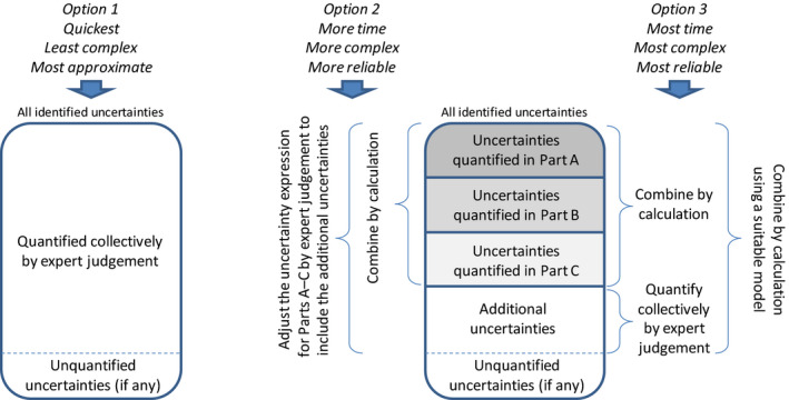
Illustration of options for characterising overall uncertainty. See text for further explanation

In some assessments, there may be some identified sources of uncertainty that the assessors are unable to include in their quantitative expression of overall uncertainty (Section 5.12): this is also illustrated in Figure 3. When this happens, the unquantified uncertainties must be characterised qualitatively and reported alongside the quantitative expression of uncertainty. The quantitative expression will then be conditional on the assumptions that have been made about these unquantified uncertainties. This has major implications for decision‐making, so assessors should try to include as many uncertainties as possible in their quantitative expression (see Section 5.13).

14.1. Option 1 – quantifying all uncertainties by expert judgement

In assessments where the uncertainty analysis has not been divided into parts, assessors should quantify the collective impact of as many as possible of the identified uncertainties directly, by expert judgement. The judgements should be made as described in Section 14.4. If assessors find it too challenging to express their judgement of the overall uncertainty as a distribution, it may be sufficient to give an approximate probability, e.g. using the approximate probability scale (Section 11.3.3).

14.2. Option 2 – incorporating additional uncertainties by expert judgement

Options 2 and 3 can be used in assessments where the uncertainty analysis has been divided into parts, and the assessors have quantified and combined at least some of the uncertainties in at least some parts of the assessment earlier in the uncertainty analysis. The task that remains is to characterise the overall uncertainty, including those already quantified and the additional uncertainties that are not yet quantified. Some of the additional uncertainties may be uncertainties that were not included in the parts that were previously quantified, while others may relate to the model used for combining the parts. In Option 2, the contribution of the additional uncertainties is combined with the previously quantified uncertainties by expert judgement. Expert judgement is simpler, because it does not require explicit specification of a model for combining the uncertainties by calculation, but is more approximate because the combination must be done by subjective judgement.

If the assessors judge that all the additional sources of uncertainty are so unimportant that, collectively, they would make no difference to the probability, probability bound or distribution obtained for the sources of uncertainty that have been quantified previously, then the latter can be taken as representing the overall uncertainty from all those sources that have been identified. This is the simplest form of the option where the additional uncertainties are incorporated by expert judgement rather than calculation. However, it should only be done if there is good reason to believe the additional uncertainties make no difference, and the basis for this must be documented and justified.

In other cases, where the additional uncertainties are judged to contribute to the magnitude of overall uncertainty, this contribution will need to be quantified. In Option 2, this is achieved by adjusting the quantitative expression for uncertainties considered earlier in the assessment, in such a way as is judged to take account of the contribution of the additional uncertainties. This can be done by judging by how much the probability for a question of interest, or the probability in a probability bound for a quantity of interest, needs to be changed to represent the contribution of the additional uncertainties. For quantities of interest, an alternative is for assessors to judge by how much the distribution accounting for the previously quantified sources of uncertainty should be changed to allow for the effect of the additional sources of uncertainty. In all cases, account should be taken of any dependencies involved. These judgements are challenging and necessarily approximate, but are much better than ignoring the additional uncertainties, which would at best be untransparent and at worst negligent (if it caused a significant under/overestimation of risk). If assessors find it too challenging to express their judgement of the adjusted uncertainty expression as a precise probability or distribution, it may be sufficient to give an approximate probability, e.g. using the approximate probability scale (Section 11.3.3).

14.3. Option 3 – incorporating additional uncertainties by calculation

This option involves judging the impact of the additional uncertainties as an additive or multiplicative factor on the scale of the quantity being assessed, expressed as a distribution or probability bound, and then combining this by calculation with the quantitative expression for uncertainties that were quantified and combined earlier in the assessment. This is analogous to the well‐established practice of using additional assessment factors to allow for additional sources of uncertainty. For example, EFSA (2012a) endorses the use of case‐by‐case expert judgement to assign additional assessment factors to address uncertainties due to deficiencies in available data, extrapolation for duration of exposure, extrapolation from lowest observed adverse effect level (LOAEL) to no observed adverse effect level (NOAEL) and extrapolation from severe to less severe effects. However, the approach proposed here is more rigorous and transparent because it makes explicit the probability judgements that are implied when using such assessment factors.

Option 3 seems less useful when the subject of assessment is a yes/no question. This is because it seems likely that experts would find it easiest to judge the necessary adjustment by thinking first about what the calculated probability needs to be adjusted to and then back‐calculating, so there is no advantage over eliciting the adjusted probability directly.

14.4. Methods for expert judgement when characterising overall uncertainty

All three options described above necessarily involve expert judgements. These expert judgements should be made using a method appropriate to the case in hand. Where an approximate judgement of the overall uncertainty is sufficient to show it is too small to make a difference to decision‐making, it may be obtained by the simpler method of expert group judgement, based on structured discussion within a normal expert group meeting (see Section 9). Where the overall uncertainty is large enough that it may make a difference to decision‐making, then it would be advisable to use a semi‐formal or formal method of expert knowledge elicitation (Sections 11.3.1 and 11.3.2). It may be efficient to start by using expert group judgement, and use this to decide whether a more formal approach is needed.

In all cases, information about the identified uncertainties needs to be provided to the experts in a form that helps them to make careful and balanced judgements: this may be aided by structured listing of the uncertainties (e.g. according to the parameter or part of the assessment each affects) and a description or graphic of the conceptual model for the assessment, to help the experts judge how the uncertainties combine. If any of the uncertainties have been evaluated qualitatively, e.g. using ordinal scales, NUSAP or uncertainty tables (Sections 10.2 and 10.1, 10.2, 10.6), experts may find it helpful to review this when making their quantitative judgement of the overall uncertainty.

All of the options discussed above involve inherently difficult and approximate judgements about how multiple uncertainties combine, including the impact of any dependencies between them. This is one of the reasons for prioritising the largest sources of uncertainty when dividing the uncertainty analysis into parts, so that they can be combined by calculation which is more reliable. This reduces the sensitivity of the final uncertainty analysis to the approximate nature of the collective quantification of the additional uncertainties.

In principle, all three options introduce additional uncertainties, in the judgements made about the additional uncertainties. This might be thought to lead to an ‘infinite regress’ in which each judgement about additional uncertainties creates further additional uncertainties. The practical solution to this is to take the uncertainty of judging the additional uncertainties into account as part of the judgement. Although this sounds challenging, assessors can do this by first considering what range or distribution would represent their judgement of the additional uncertainties, and then considering whether that range or distribution needs to be changed to represent their uncertainty in (a) making that judgement and (b) combining it with the previously quantified sources of uncertainty (whether by expert judgement or calculation). When doing this, the assessors should also make one last check for any further additional uncertainties that have not yet been included, and take them into account in the final characterisation of overall uncertainty.

15. Reporting uncertainty analysis in scientific assessments

This section repeats what is written in the guidance document (EFSA Scientific Committee, 2018) and is included here for completeness.

For standardised assessments where no case‐specific sources of uncertainty have been identified, the EFSA output must at minimum state what standardised procedure was followed and report that non‐standard uncertainties were checked for and none were found. If the applicability of the standardised procedure to the case in hand is not self‐evident, then an explanation of this should be provided.

In all other assessments, the uncertainty analysis should be reported as described below, although the level of detail may be reduced due to time constraints in urgent assessments.

In standardised assessments where non‐standard uncertainties are found, the assessors should report that standard uncertainties in the assessment are accepted to be covered by the standardised procedure and the uncertainty analysis is therefore restricted to non‐standard uncertainties that are particular to this assessment, the analysis of which should then be reported as described below.

Uncertainty analysis is part of scientific assessment, so in all cases, it should be reported in a manner consistent with EFSA's general principles regarding transparency (EFSA, 2007, 2009) and reporting (EFSA, 2014b, 2015a). In particular, it is important to list the sources of uncertainty that have been identified and document how they were identified, how each source of uncertainty has been evaluated and how they have been combined, where and how data and expert judgement have been used, what methodological approaches have been used (including models of any type) and the rationale for choosing them, and what the results were. Where the assessment used methods that are already described in other documents, it is sufficient to refer to those.

The location of information on the uncertainty analysis within the assessment report should be chosen to maximise transparency and accessibility for readers. This may be facilitated by including one or more separate sections on uncertainty analysis, which are identifiable in the table of contents.

The Scientific Committee has stated that EFSA's scientific assessments must report clearly and unambiguously what sources of uncertainty have been identified and characterise their overall impact on the assessment conclusion, in a form compatible with the requirements of decision‐makers and any legislation applicable to the assessment in hand (Section 1.4). In some types of assessment, decision‐makers or legislation may stipulate a specified form for reporting assessment conclusions. In some cases, this may comprise qualitative descriptors such as ‘safe’, ‘no concern’, ‘sufficient evidence’. To enable these to be used by assessors without implying risk management judgements requires that assessors and decision‐makers have a shared understanding or definition of the question or quantity of interest which the qualitative descriptor refers to, and the level of certainty associated with the qualitative descriptor. In other cases, decision‐makers or legislation may require that conclusions be stated without qualification by probability expressions. This can be done if assessors and decision‐makers have a shared understanding or definition of the level of probability required for practical certainty about a question of interest, i.e. a level of probability that would be close enough to 100% (answer certainly yes) or 0% (answer certainly no) for decision‐making purposes. On issues where practical certainty is not achieved, the assessors would report that they cannot conclude, or that the assessment is inconclusive.

In such cases, assessors should also comply with any requirements of decision‐makers or legislation regarding where and how to document the details of the uncertainty analysis that led to the conclusion.

In other cases, where the form for reporting conclusions is not specified by decision‐makers or legislation, the assessment conclusion should include (a) a clear statement of the overall result for those uncertainties that have been quantified and (b) a clear description of unquantified sources of uncertainty, i.e. those that could not be included in the quantitative analysis. The former will generally express the overall quantified uncertainty about the assessment conclusion using probabilities, probability distributions, probability bounds, or ranges from the approximate probability scale (see Sections 5.11 and 11.3.3). For each unquantified source of uncertainty, the assessors should describe (either in the conclusion or another section, as appropriate) which part(s) of the assessment it arises in, the nature of the uncertainty (e.g. whether it is an instance of ambiguity, complexity or lack of knowledge), the cause or reason for it, how it affects the assessment (but not how much), why it is difficult to quantify, what assumptions have been made about it in the assessment, and what could be done to reduce or better characterise it. Assessors must avoid using any words that imply a judgement about the magnitude or likelihood of the unquantified sources of uncertainty (Section 5.12).

In addition to the detailed reporting of the methods and results of the uncertainty analysis, the assessors should prepare a concise summary of the overall characterisation of uncertainty in format and style suitable for inclusion in the executive summary of the assessment report. This should present, in the simplest terms possible, a quantitative expression of the combined effect on the assessment conclusion of those uncertainties that have been quantified, and a brief description of any unquantified sources of uncertainty.

Assessors must check that there is no incompatibility between the reporting of the uncertainty analysis and the assessment conclusions. In principle, no such incompatibility should occur, because sound scientific conclusions will take account of relevant uncertainties, and therefore should be compatible with an appropriate analysis of those uncertainties. If there appears to be any incompatibility, assessors should review and if necessary revise both the uncertainty analysis and the conclusion to ensure that they are compatible with one another and with what the science will support.

In many assessments, information on the main contributors to the uncertainty of the question or quantity of interest may be useful to decision‐makers, to inform decisions about the need for further work such as data gathering, to support refinement of the assessment. Such information may be generated by methods for prioritising uncertainties (see Section 12).

16. Communicating scientific uncertainties

16.1. EFSA's risk communication mandate

EFSA is mandated to ‘be an independent scientific source of advice, information and risk communication in order to improve consumer confidence’. Creating and sustaining such confidence requires coherence and co‐ordination of all three outputs: advice, information and risk communication. The quality, independence and transparency of EFSA's scientific advice and information, supported by the robustness of the working processes needed to develop them, are critical for effective risk communication and for ensuring public confidence. Equally, clear and unambiguous communication of assessment conclusions contextualises the scientific advice and information, aiding political decision‐makers to prioritise policy options and take informed decisions. Through multipliers (e.g. media, NGOs) this also forms a basis for consumers’ greater confidence in their own choices and in risk management action.

Therefore, EFSA communicates the results of its scientific assessments to decision‐makers, stakeholders (e.g. consumer/non‐governmental organisations, media, food chain operators), and the public at large. Besides the huge cultural, linguistic and social diversity in the EU, there is also a vast spectrum of individual needs, values and technical knowledge among these target audiences. Decision‐makers and stakeholders are also responsive to the perceptions of the general public. Effective risk communication, therefore, requires a commonly understood vocabulary, careful crafting of messages and selection of tools keeping in mind the characteristics of the target audience and the perceived sensitivities of the topic.

To be useful to decision‐makers, ensure coherence and limit possible misinterpretation of its scientific assessments, EFSA communicates its scientific results in a manner that aims to be both meaningful to specialists and understandable to informed laypersons. Currently, EFSA does not usually tailor different messages about the same scientific output to different audiences in a wholly structured way. Instead, a variety of communications channels and media, ranging from the simple to the complex, are used to highlight the same messages to different audiences, regardless of the levels of scientific knowledge.

16.2. Risk perception and uncertainty

Perceptions of the risks or benefits for which EFSA is providing an assessment and the meaningful expression of the identified sources of uncertainty, play paramount roles in how recipients of EFSA's communication act upon the results. This varies by target audience and their respective level of technical knowledge.

Understanding of the type and degree of uncertainties identified in the assessment helps to characterise the level of risk to the recipients and is therefore essential for informed decision‐making. Communication helps them to understand the range and likelihood of possible consequences. This is especially useful for technical and political decision‐makers. For audiences with less technical understanding of the topic under assessment, increasing awareness of scientific uncertainties could in some cases reduce the individual's confidence in their own decision‐making or in decisions made by public authorities. Yet, in some cultural contexts, communication of the uncertainties to non‐technical audiences is received positively because of the greater transparency of the process, even if it makes decisions more difficult. The potential decrease in confidence is offset by an increase in trust.

The main roles of risk communication within this process are to contextualise the uncertainties in relation to the perceived risks, to underline the transparency of the process and to explain how scientists can address the information gaps in the future (for example, recommendations on data collection, research priorities).

16.3. Challenges of communicating uncertainty in scientific assessments

Communicating scientific uncertainty requires both simplifying and complicating the normal scientific discourse (Fischhoff and Davis, 2014). Various arguments have been made both for and against communicating uncertainty to the general public (Johnson and Slovic, 1995, 1998). Yet, there is little empirical evidence to support either view (Miles and Frewer, 2003).

In terms of the best methods, the literature is equivocal about the advantages and/or disadvantages of communicating uncertainty to stakeholders in qualitative or quantitative terms. Although the uncertainty analysis is preferably quantitative, quantification can give an exaggerated impression of accuracy. Therefore, it is often expressed qualitatively in risk communication. However, qualitative terms are understood differently by different people and always entail a judgement.

From EFSA's perspective, communicating scientific uncertainties is crucial to its core mandate, reaffirming its role in the Risk Analysis process. As a public institution, EFSA is obliged to be open and transparent to the public. In addition the clear and unambiguous communication of scientific uncertainty is an enabling mechanism, providing decision‐makers with the scientific grounds for risk‐based decision‐making. It increases transparency both of the assessments and of the resulting decision‐making, ensuring that confidence in the scientific assessment process is not undermined.

As a consequence decision‐makers are better able to take account of the uncertainties in their risk management strategies and to explain, as appropriate, how scientific advice is weighed against other legitimate factors. Explaining how decisions or strategies take account of scientific uncertainties will contribute to increased public confidence in the EU food safety system as well.

Although EFSA regularly communicates the scientific uncertainties related to its assessments in its scientific outputs and in its non‐technical communication activities, it has not applied a model consistently across the organisation.

Overall, while developing this document, EFSA identified a need to differentiate more systematically the level of scientific technicality in the communications messages on uncertainties intended for different target audience. This more differentiated and structured approach marks a shift from the current one described in 16.1 above.

16.4. Towards best practice for communicating uncertainty

As indicated above the literature is equivocal about the most effective strategies to communicate scientific uncertainties. The IPCC recommends use of reciprocal statements to avoid value‐laden interpretations: ‘the way in which a statement is framed will have an effect on how it is interpreted (e.g. a 10% chance of dying is interpreted more negatively than a 90% chance of surviving)’ (Mastrandrea et al., 2010). According to IPCS, ‘it would be valuable to have more systematic studies on how risk communication of uncertainties, using the tools presented […] functions in practice, regarding both risk managers and other stakeholders, such as the general public’ (IPCS, 2014). Some scientific assessment and industry bodies have compiled case study information to develop a body of reference materials (BfR, 2013; ARASP, 2015). But, on the whole there is a lack of empirical data in the literature on which to base a working model. In relation to food safety in Europe, more expertise is needed for structured communication on uncertainty.

The development of effective communications messages requires an in‐depth knowledge of target audiences including: their level of awareness and understanding of food safety issues; their attitudes to food in general and food safety in particular; the possible impact of communications on behaviour; the appropriate channels for effective dissemination of messages; and – in relation to scientific uncertainties – the appropriate language to understand and benefit from receiving uncertainty information such as probabilities. Therefore, while EFSA's scientific Panels piloted the draft Guidance on uncertainty, EFSA conducted two target audience research projects on communicating scientific uncertainty among its institutional partners (European Commission, European Parliament, Member States) and its stakeholders (consumer organisations, non‐governmental organisations, food chain operators, scientists, media, the general public).

In a first pilot study using focus groups, the responses of and discussions among individuals directly involved in using EFSA's scientific advice – risk managers (i.e. technical decision‐makers), political decision‐makers, non‐governmental organisations, food chain operators – and members of the general public, were evaluated to ascertain their understanding and use of different types of uncertainty expressions (e.g. qualitative, quantitative, positively framed, negatively framed), and the effects this information might have on their risk perceptions as well as on their trust in scientific advisory bodies such as EFSA. A second follow‐up study was conducted online, in six different European languages and promoted by the communications departments of eight EU national risk assessment bodies belonging to EFSA's Communications Expert Network. With over 1,900 respondents taking part, the results of this online survey broadened the sample pool, further tested the indications from the initial study and provided insights on additional aspects, including how language/culture may influence people's preferences for uncertainty information.

The two studies resulting from this research (EFSA, 2018a; ICF, 2018) provided a rich source of quantitative and qualitative data with which to complement the academic literature on best practices for communicating scientific uncertainties to different audiences. As a consequence of these activities, the Scientific Committee decided in March 2017 to develop a Companion Guidance document on Communicating Uncertainty in Scientific Assessments (EFSA, 2018b),6 aimed at communications practitioners at EFSA and in other organisations working in the food safety, public health and related areas. The Companion Guidance provides practical advice and tools for communicators to explain the significance of the different outputs (e.g. probability distribution, verbal statement) resulting from the types of uncertainty analysis described above in this document, with different target audiences in mind. The Companion Guidance will be applied to EFSA's risk communication activities simultaneously with the implementation of the Guidance document in EFSA's scientific assessments.

17. Way forward and recommendations

This document presents the principles and methods behind the concise guidance document which is intended to guide EFSA panels and staff on how to deal with sources of uncertainty in scientific assessments. Together, the two documents provide a toolbox of methods, from which assessors can select those methods which most appropriately fit the purpose of their individual assessment.

While leaving flexibility in the choice of methods, all EFSA scientific assessments must include consideration of uncertainty. For reasons of transparency, all assessments must report clearly and unambiguously the impact of uncertainty on the assessment conclusion. In assessments where the impact of one or more uncertainties cannot be characterised it must be reported that this is the case and that consequently, the assessment conclusion is conditional on assumptions about those uncertainties, which should be specified.

It is expected that closer interaction will be needed between assessors and decision‐makers both during the assessment process and when communicating the conclusions.

It is recommended that a specific plan for the implementation of the Guidance should be drafted.

Furthermore, the following recommendations are made to support implementation of the Guidance:

1. EFSA should initiate further work to explore best practices and develop further guidance in areas where this will benefit implementation of the Guidance, including types of expert elicitation not covered by EFSA (2014a,b) (e.g. for variables, dependencies, yes/no questions and approximate probabilities).

2. Panels should be encouraged to develop sector‐specific uncertainty guidance document(s) or incorporate relevant approaches from the Guidance into their existing sector‐specific guidance, where this would be helpful.

3. Panels should develop Panel‐specific lists of standard and/or non‐standard uncertainties where this is helpful for use in their assessments. Listing standard uncertainties may also help to prioritise standardised procedures for review and calibration.

4. International collaboration will be needed to calibrate standardised procedures that use internationally agreed approaches. Consideration could be given to initiating this by means of an international workshop on uncertainty analysis.

5. It is recommended that at least one assessor in each Panel and Working Group should have received Panel‐specific training in the use of the Guidance, and that all assessors should have basic training in probability judgements.

6. Some methods for uncertainty analysis require specialist expertise in statistics, modelling or expert knowledge elicitation. This should be provided by including relevant experts in Working Groups where needed, or as internal support from EFSA.

7. It is recommended that EFSA establish a Standing Working Group on uncertainty analysis to provide advice, mentoring and support to Panels and Working Groups as they implement the Guidance.

8. It is recommended that EFSA establish a central repository to collect examples of the application of the Guidance to different types of assessment in different areas of EFSA's work, which will provide a helpful resource to assessors and facilitate sharing of lessons learned.

Abbreviations

ADI

acceptable daily intake

AF

assessment factor

AHAW

EFSA Panel on Animal Health and Welfare

ANOVA

analysis of variance

ANS

EFSA panel on Food Additives and Nutrient Sources added to Food

ANSES

French Agency for Food, Environmental and Occupational Health & Safety

ARASP

Center for Advancing Risk Assessment Science and Policy

BBNs

Bayesian belief networks

BEA

break‐even analysis

BfR

Bundesinstitut für Risikobewertung, Germany

BIOHAZ Panel

EFSA Panel on Biological Hazards

BMDL

benchmark dose modelling

BPA

bisphenol A

BSE

bovine spongiform encephalopathy

bw

body weight

CAT

Critical Appraisal Tool

CDC

Centre for Disease Control and Prevention

CDF

cumulative density function

CONTAM

EFSA Panel on Contaminants

CSAF

chemical‐specific adjustment factor

ECHA

European Chemicals Agency

EKE

expert knowledge elicitation

EPA

Environmental Protection Agency

FAO

Food and Agriculture Organization of the United Nations

FAST

Fourier amplitude sensitivity test

FDA

Food and Drug Administration us

FERA

Food and Environmental Research Agency UK

FOCUS

FOrum for Co‐ordination of pesticide fate models and their USe

GM

genetically modified

HDMI

Target human dose

IESTI

International Estimate of Short‐Term Intake

IPCC

Intergovernmental Panel on Climate Change

IPCS

International Programme on Chemical Safety

IRGC

International Risk Governance Council

JECFA

Joint FAO/WHO Expert Committee on Food Additives

JEMRA

Joint FAO/WHO Expert Meetings on Microbiological Risk Assessment

JMPR

Joint FAO/WHO Meeting on Pesticide Residues

LOAEL

lowest observed adverse effect level

LOD

limit of detection

LoE

lines of evidence

MC

Monte Carlo

MCF

Monte Carlo filtering

MOS

margins of safety

NOAEL

no observed adverse effect level

NQ

not quantified

NRC

National Research Council

NRSA

nominal range sensitivity analysis

NUSAP

Numeral, Unit, Spread, Assessment and Pedigree

OIE

World Organisation for Animal Health

PCC

partial correlation coefficient

PDF

probability density function

PLH Panel

EFSA Panel on Plant Health

PNEC

predicted no effect concentration

POD

point of departure

PPR Panel

EFSA Panel on Plant Protection Products and their Residues

PRAS Unit

EFSA Pesticides and Residues Unit

PRCC

partial rank correlation coefficient

RA

risk assessment

RIVM

National Institute for Public Health and the Environment

RQ

risk quotient

SA

sensitivity analysis

SC

Scientific Committee of EFSA

SCCS

Scientific Committee on Consumer Safety

SCENIHR

Scientific Committee on Emerging and Newly Identified Health Risks

SCHER

Scientific Committee on Health and Environmental Risks

SCF

Scientific Committee for Food

SF

safety factor

SRC

standardised regression coefficient

SRRC

standardised rank regression coefficient

St.dev

standard deviation

SU

sampling for uniformity

TDI

tolerable daily intake

TER

toxicity–exposure ratio

ToR

Terms of Reference

wc

worst case

WHO

World Health Organization

Glossary

Additional uncertainties

Term used when some uncertainties have already been quantified, to refer to other uncertainties that have not yet been quantified and need to be taken into account in the characterisation of overall uncertainty.

Aleatory uncertainty

Uncertainty caused by variability, e.g. uncertainty about a single toss of a coin, or the exposure of a randomly selected member of a population.

Ambiguity

The quality of being open to more than one interpretation. A type or cause of uncertainty that may apply, for example, to questions for assessment, evidence, models or concepts, and assessment conclusions.

Approximate probability

A range or bound for a probability.

Approximate probability scale

A set of approximate probabilities with accompanying verbal probability terms, shown in Section 12.3 of the Guidance and recommended for harmonised use in EFSA scientific assessments.

Assessment conclusion

The answer provided by a scientific assessment to the question it addresses, including characterisation of the overall uncertainty (q.v.).

Assessment factor

A numerical factor used in quantitative assessment, to represent or allow for extrapolation or uncertainty. Related terms: safety factor, uncertainty factor.

Assessment input

Inputs to a calculation or model, including any data, assessment factors, default values, assumed values expert judgements.

Assessment output

The output of a calculation or model.

Assessment question

The question to be addressed by a scientific assessment. Assessment questions may be quantitative (estimation of a quantity) or categorical (e.g. yes/no questions).

Assessor

A person conducting a scientific assessment and/or uncertainty analysis.

Bayesian inference

A form of statistical inference in which probability distributions are used to represent uncertainty.

Bound

The upper or lower limit of a range of possible numbers, or of an approximate probability.

Calibration

Used in the Guidance to refer to the process of evaluating whether a standardised procedure is appropriately conservative and, if necessary, adjusting it to achieve this. More specifically, the process of ensuring a standard procedure provides an appropriate probability of achieving a specified management objective to an acceptable extent.

Case‐specific assessment

Scientific assessments where there is no pre‐established standardised procedure, so the assessors have to develop an assessment plan that is specific to the case in hand. Standardised elements (e.g. default values) may be used for some parts of the assessment, but other parts require case‐specific approaches. Both standardised and case‐specific assessments are used in Applications Management, one of the core processes in EFSA's Process Architecture.

Categorical question

An assessment question that is expressed as a choice between two or more categories, e.g. yes/no or low/medium/high. Many issues that are expressed as categorical questions refer explicitly or implicitly to quantities (e.g. whether exposure is below a threshold value).

Characterising uncertainty

The process of making and expressing an evaluation of uncertainty either for an assessment as a whole or for a specified part of an assessment. Can be performed and expressed either qualitatively or quantitatively.

Chemical‐specific adjustment factor (CSAF)

A quantitative measurement or numerical parameter estimate that replaces a default uncertainty subfactor.

Collective

Used in this document to refer to evaluating the combined impact of two or more uncertainties together.

Combine uncertainties

The process of integrating separate characterisations of two or more uncertainties to produce a characterisation of their combined impact on an assessment or part of an assessment. Can be performed by calculation or expert judgement, and in the latter case either quantitatively or qualitatively.

Combined uncertainty

Expression of the combined impact of multiple sources of uncertainty on the conclusion of an assessment or part of an assessment.

Conceptual model

The reasoning developed by assessors in the course of a scientific assessment, which is then implemented as a narrative argument, a logic model, a calculation or a combination of these. Documenting the conceptual model, e.g. as a bullet list, flow chart or graphic, may be helpful to assessors during the assessment and also for readers, if included in the assessment report.

Conditional

Used in the Guidance to refer to dependence of the quantitative result of an assessment or uncertainty analysis on assumptions made about sources of uncertainty that have not been quantified.

Confidence (interval)

Levels of confidence (e.g. high, low) are often used to express the probability that a conclusion is correct. In frequentist statistics, a confidence interval is a range that would include the true value of the parameter to be estimated in a specified proportion of occasions if the experiment and/or statistical analysis that produced the range was repeated an infinite number of times. In Bayesian statistics it is replaced with credible interval, which is a range within which the true value would lie with specified probability. In a social science context, confidence is the expectation of an outcome based on prior knowledge or experience.

Conservative

Term used to describe assessments, or parts of assessments (e.g. assumptions, default factors), that tend to overestimate the severity and/or frequency of an adverse consequence (e.g. overestimate exposure or hazard and consequently risk). Can also be used to refer to underestimation of a beneficial consequence. Conservatism is often introduced intentionally, as a method to allow for uncertainty.

Coverage

Used in this document to refer to the probability that the real value of a quantity is less adverse than a given estimate of that quantity. A conservative estimate is one providing a level of coverage considered adequate by decision‐makers. The term coverage is used with a broader meaning in statistics.

Credible interval

A range for a non‐variable quantity which has a specified probability of including the true value of the quantity. See also ‘confidence’ and ‘probability bound’.

Decision criteria

Numerical criteria (sometimes called ‘trigger values’) used in some parts of EFSA for deciding what conclusion can be made on risk and/or whether further assessment is needed. In some cases (e.g. pesticides), provision for uncertainty is built into the trigger value instead of, or as well as, being built into the assessment or its inputs.

Decision‐maker

A person with responsibility for making decisions; in the context of this document, a person making decisions informed by EFSA's scientific advice. Includes risk managers but also people making decisions on other issues, e.g. health benefits, efficacy.

Deep uncertainty

A source or sources of uncertainty, the impact of which on the assessment the assessor(s) is not able to quantify.

Default value or factor

Pragmatic, fixed or standard value used in the absence of relevant data, implicitly or explicitly regarded as accounting appropriately for the associated uncertainty.

Dependency

Variable quantities are dependent when they are directly or indirectly related, such that the probability of a given value for one quantity depends on the value(s) of other quantities (e.g. food consumption and body weight). Sources of uncertainty are dependent when learning more about one would alter the assessors’ uncertainty about the other.

Deterministic

A deterministic calculation uses fixed numbers as input and will always give the same answer, in contrast to a probabilistic calculation where one or more inputs are distributions and repeated calculations result in different output and different uncertainty.

Distribution

A probability distribution is a mathematical function that relates probabilities with specified intervals of a continuous quantity or values of a discrete quantity. Applicable both to random variables and uncertain parameters.

Distribution parameters

Numbers which specify a particular distribution from a family of distributions.

Epistemic uncertainty

Uncertainty due to limitations in knowledge.

Evidence appraisal

The process of evaluating the internal validity of evidence and its external validity for the question at hand, in addition to other sources of uncertainties such as imprecision.

Expert

A knowledgeable or skilled person.

Expert group judgement

The process of eliciting a judgement or judgements from a group of experts without using a formal or semi‐formal elicitation procedure.

Expert judgement

The judgement of a person with relevant knowledge or skills for making that judgement.

Expert knowledge elicitation (EKE)

A systematic, documented and reviewable process to retrieve expert judgements from a group of experts, often in the form of a probability distribution.

External validity

Extent to which the findings of a study can be generalised or extrapolated to the assessment question at hand. It is not an inherent property of the evidence.

Frequency

The number of occurrences of something, expressed either as the absolute number or as a proportion or percentage of a larger population (which should be specified)

Identifying uncertainties

The process of identifying sources of uncertainty affecting a scientific assessment.

Ignorance

Absence of knowledge, including ‘unknown unknowns’.

Individual expert judgement

The process of eliciting a judgement or judgements from a single expert without using a formal or semi‐formal elicitation procedure.

Infinite regress

In relation to uncertainty, refers to the problem that assessment of uncertainty is itself uncertain, thus opening up the theoretical possibility of an infinite series of assessments, each assessing the uncertainty of the preceding one. See Section 14.4 for proposed solution in the context of this document.

Influence analysis

The extent to which plausible changes in the overall structure, parameters and assumptions used in an assessment produce a change in the results.

Internal validity

Extent to which systematic error is minimised by the study design. It is an inherent property of evidence.

Likelihood

In everyday language, refers to the chance or probability of a specific event occurring: generally replaced with ‘probability’ in this document. In statistics, maximum likelihood estimation is one option for obtaining confidence intervals (Annex B.10). In Bayesian statistics, the likelihood function encapsulates the information provided by the data (Annex B.12).

Line of evidence

A set of evidence of similar type.

Logic model

A model expressing a yes/no conclusion as a logical deduction from the answers to two or more yes/no questions.

Management objective

A well‐defined expression of the outcome required by decision‐makers from a decision, policy or procedure, specifying the question or quantity of interest and the temporal and spatial scale for which it should be assessed. Applied in the Guidance to the calibration of standardised procedures.

Markov Chain Monte Carlo

A form of Monte Carlo where values are not sampled independently but instead are sampled from a Markov chain. In many situations where standard Monte Carlo is difficult or impossible to apply, MCMC provides a practical alternative.

Model

In scientific assessment, usually refers to a mathematical or statistical construct, which is a simplified representation of data or of real world processes, and is used for calculating estimates or predictions. Can also refer to the structure of a reasoned argument or qualitative assessment.

Model uncertainty

Bias or imprecision associated with compromises made or lack of adequate knowledge in specifying the structure of a model, including choices of mathematical equation or family of probability distributions. Can also refer to limitations in knowledge affecting the construction of a reasoned argument or qualitative assessment.

Monte Carlo

A method for making probability calculations by random sampling from distributions.

Monte Carlo: 1D

A method for making probability calculations by random sampling from one set of distributions, all representing uncertainty about non‐variable quantities or categorical questions.

Monte Carlo: 2D

A method for making probability calculations by random sampling from two sets of distributions, one set describing the variability of variable quantities, and the second set representing uncertainty, including uncertainty about the parameters of the distributions describing variability.

Non‐standard uncertainties

Any deviations from a standardised procedure or standardised assessment element that lead to uncertainty regarding the result of the procedure. For example, studies that deviate from the standard guidelines or are poorly reported, cases where there is doubt about the applicability of default values, or the use of non‐standard or ‘higher tier’ studies that are not part of the standard procedure.

Non‐variable quantity

A quantity that has a single real or true value.

Ordinal scale

A scale of measurement comprised of ordered categories, where the magnitude of the difference between categories is not quantified.

Overall uncertainty

The assessors’ uncertainty about the question or quantity of interest at the time of reporting, taking account of the combined effect of all sources of uncertainty identified by the assessors as being relevant to the assessment.

Parameter

Parameter is used in this document to refer to quantitative inputs to an assessment or uncertainty analysis, without specifying whether they are variable or not. In most places a non‐variable quantity is implied, consistent with the use of parameter in statistics. However, in some places parameter could refer to a variable quantity, as it is sometimes used in biology (e.g. glucose level is referred to as a blood parameter).

Parts of the scientific assessment

Components of a scientific assessment that it is useful to distinguish for the purpose of assessment, e.g. a risk assessment comprises hazard and exposure assessment, and each of these can be subdivided further (e.g. to distinguish individual model parameters, studies, or lines of evidence).

Parts of the uncertainty analysis

Parts of an uncertainty analysis that it is useful to distinguish, evaluating uncertainties within each part collectively, and then combining the parts and any additional uncertainties to characterise overall uncertainty. Not necessarily the same as the parts into which the scientific assessment is divided (see text).

Practical certainty

A level of probability that would be close enough to 100% (answer is certain to be yes) or 0% (certain to be no) for the purpose of decision‐making. What levels of probability will comprise practical certainty will vary, depending on the context for the decision including the decision options and their respective costs and benefits.

Prior distribution

In Bayesian inference, a probability distribution representing uncertainty about parameters in a statistical model prior to observing data. The distribution may be derived from expert judgements based on other sources of information.

Prioritising uncertainties

The process of evaluating the relative importance of different sources of uncertainty, to guide decisions on how to treat them in uncertainty analysis or to guide decisions on gathering further data with the aim of reducing uncertainty. Prioritisation is informed by influence or sensitivity analysis.

Probabilistic

(1) Representation of uncertainty and/or variability using probability distributions. (2) Calculations where one or more inputs are probability distributions and repeated calculations give different answers. Related term: deterministic.

Probability

Defined depending on philosophical perspective: (1) the frequency with which sampled values arise within a specified range or for a specified category; (2) quantification of judgement regarding the likelihood of a particular range or category.

Probability bound

A probability or approximate probability for a specified range of values.

Probability bounds analysis

A method for combining probability bounds for inputs in order to obtain a probability bound for the output of a deterministic model. It is a special case of the general theory of imprecise probability which provides more ways to obtain partial expressions of uncertainty for the output based on more general partial expressions for inputs.

Probability judgement

A probability, approximate probability or probability bound obtained by expert judgement.

Propagation of uncertainty

Propagation refers to the process of carrying one or more uncertainties through an assessment in order to evaluate their impact on the assessment conclusion. It may be done by calculation or expert judgement.

Protection goal

A management objective for protection of an entity of interest.

Qualitative assessment

Sometimes refers to the form in which the conclusion of an assessment is expressed (e.g. a verbal response to a question of interest), or to the methods used to reach the conclusion (not involving calculations), or both.

Qualitative expression of uncertainty

Expression of uncertainty using words or ordinal scales.

Quantitative assessment

Sometimes refers to the form in which the conclusion of an assessment is expressed (i.e. quantitatively), or to the methods used to reach the conclusion (involving calculations), or both.

Quantitative expression of uncertainty

Expression of uncertainty using numeric measures of the range and relative likelihood of alternative answers or values for a question or quantity of interest.

Quantitative question

A question requiring estimation of a quantity. E.g. estimation of exposure or a reference dose, the level of protein expression for a GM trait, the infective dose for a pathogen, etc.

Quantity

A property or characteristic having a numerical scale.

Quantity of interest

A quantity that is the subject of a scientific assessment as a whole, or of a part of such an assessment.

Question of interest

A categorical question that is the subject of a scientific assessment as a whole, or of a part of such an assessment.

Range

A set of continuous values or categories, specified by an upper and lower bound

Real value

A synonym for true value (q.v.).

Resolved

The actual or hypothetical process of removing an uncertainty by making the measurement or observation needed to obtain the true answer or value for the question or quantity of interest.

Risk analysis

A process consisting of three interconnected components: risk assessment, risk management and risk communication.

Risk assessment

A scientifically based process consisting of four steps: hazard identification, hazard characterisation, exposure assessment and risk characterisation.

Risk communication

The interactive exchange of information and opinions throughout the risk analysis process as regards hazards and risks, risk‐related factors and risk perceptions, among risk assessors, risk managers, consumers, feed and food businesses, the academic community and other interested parties, including the explanation of risk assessment findings and the basis of risk management decisions.

Risk management

The process, distinct from risk assessment, of weighing policy alternatives in consultation with interested parties, considering risk assessment and other legitimate factors, and, if need be, selecting appropriate prevention and control options.

Risk management judgement

The process or result of weighing policy alternatives in consultation with interested parties, considering risk assessment and other legitimate factors, and, if need be, selecting appropriate prevention and control options.

Risk manager

A type of decision‐maker, responsible for making risk management judgements

Scientific assessment

The process of using scientific evidence and reasoning to answer a question or estimate a quantity.

Scope (for non‐standard uncertainties)

The degree to which a standardised procedure was calibrated to be more conservative than required (e.g. by rounding up an assessment factor), which determines how much opportunity there will be to accommodate the presence of non‐standard uncertainties in individual assessments.

Semi‐formal expert knowledge elicitation

A structured and documented procedure for eliciting expert judgements that is intermediate between fully formal elicitation and informal expert judgements.

Sensitivity analysis

A study of how the variation in the outputs of a model can be attributed to, qualitatively or quantitatively, different sources of uncertainty or variability. Implemented by observing how model output changes when model inputs are changed in a structured way.

Severity

Description or measure of an effect in terms of its adversity or harmfulness.

Source of uncertainty

Used in this document to refer to an individual contribution to uncertainty, defined by its location (e.g. a component of the assessment) and its type (e.g. measurement uncertainty, sampling uncertainty). A single location may be affected by multiple types of uncertainty, and a single type of uncertainty may occur in multiple locations.

Standard uncertainties

Sources of uncertainty that are considered (implicitly or explicitly) to be addressed by the provisions of a standardised procedure or standardised assessment element. For example, uncertainties due to within and between species differences in toxicity are often addressed by a default factor of 100 in chemical risk assessment.

Standardised assessment

An assessment that follows a standardised procedure (q.v.).

Standardised procedure

A procedure that specifies every step of assessment for a specified class or products or problems, and is accepted by assessors and decision‐makers as providing an appropriate basis for decision‐making. Often (but not only) used in scientific assessments for regulated products. Both standardised and case‐specific assessments are used in Applications Management, one of the core processes in EFSA's Process Architecture.

Statistical model

A probabilistic model of variability, possibly modelling dependence between variables or dependence of one variable on another, for example, a family of probability distributions representing alternative possible distributions for a variable or regression or dose–response models. Usually has parameters which control the detail of distributions or dependence.

Target quantity

A quantity which it is desired to estimate, e.g. what severity and frequency of effects is of interest.

True value

The actual value that would be obtained with perfect measuring instruments and without committing any error of any type, both in collecting the primary data and in carrying out mathematical operations. (OECD Glossary of Statistical Terms, https://stats.oecd.org/glossary/detail.asp?ID=4557).

Trust (in social science)

The expectation of an outcome taking place within a broad context and not based on prior knowledge or experience.

Typology of uncertainties

A structured classification of types of uncertainties defined according to their characteristics.

Uncertainty

In this document, uncertainty is used as a general term referring to all types of limitations in available knowledge that affect the range and probability of possible answers to an assessment question. Available knowledge refers here to the knowledge (evidence, data, etc.) available to assessors at the time the assessment is conducted and within the time and resources agreed for the assessment. Sometimes ‘uncertainty’ is used to refer to a source of uncertainty (see separate definition), and sometimes to its impact on the conclusion of an assessment.

Uncertainty analysis

The process of identifying and characterising uncertainty about questions of interest and/or quantities of interest in a scientific assessment.

Uncertainty factor

A quantity used in a scientific assessment to account or allow for part or all of the uncertainty affecting that assessment. This document uses the more general term ‘assessment factor’.

Unknown unknowns

A limitation of knowledge that one is unaware of.

Unquantified uncertainty

An identified source of uncertainty in a scientific assessment that the assessors are unable to include, or choose not to include, in a quantitative expression of overall uncertainty for that assessment.

Urgent assessment

A scientific assessment requested to be completed within an unusually short period of time. Part of Urgent Responses Management in EFSA's Process Architecture

Variability

Heterogeneity of values over time, space or different members of a population, including stochastic variability and controllable variability. See Section 5.3 for discussion of uncertainty and variability.

Variable quantity

A quantity that has multiple true v/alues (e.g. body weight measured in different individuals in a population, or in the same individual at different points in time).

Weight of evidence assessment

A process in which evidence is integrated to determine the relative support for possible answers to a scientific question.

Well defined

A question or quantity of interest that has been defined by specifying an experiment, study or procedure that could be undertaken, at least in principle, and would determine the question or quantity with certainty.

Annex A – The melamine case study

A.1. Purpose of case study

Worked examples are presented in annexes to the Guidance Document, to illustrate the different approaches. To increase the coherence of the document and facilitate the comparison of different methods, a single case study was selected, which is introduced in the following section.

Presentation of the case study is arranged as follows:

• Introduction to the melamine example (this Annex, Section A.2)

• Definition of assessment questions for use in the case study (this Annex, Section A.3)

• Overview of outputs produced by the different methods (this Annex, Section A.4)

• Detailed description of how each method was applied to the example (subsections on ‘Melamine example’ within the sections on each method, in Annex B (1–17))

• Description of models used when demonstrating the quantitative methods (Annex C)

A.2. Introduction to melamine example

The example used for the case study is based on an EFSA Statement on melamine that was published in 2008 (EFSA, 2008). This Statement was selected for the case study in this document because it is short, which facilitates extraction of the key information and identification of the sources of uncertainty, and because it incorporates a range of types of uncertainties. However, it should be noted that the risk assessment in this statement has been superseded by a subsequent full risk assessment of melamine in food and feed (EFSA, 2010a,b).

While this is an example from chemical risk assessment for human health, the principles and methodologies illustrated by the examples are general and could be applied to any other area of EFSA's work, although the details of implementation would vary.

It is emphasised that the examples on melamine in this document are provided for the purpose of illustration only, and are based on information that existed when the EFSA statement was prepared in 2008. The examples were conducted only at the level needed to illustrate the principles of the approaches and the general nature of their outputs. They are not representative of the level of consideration that would be needed in a real assessment and must not be interpreted as examples of good practice. Also they must not be interpreted as a definitive assessment of melamine or as contradicting anything in any published assessment of melamine.

The case study examples were developed using information contained in the EFSA (2008) statement and other information cited therein, including a previous US FDA assessment (FDA, 2007). Where needed for the purpose of the examples, additional information was taken from EFSA (2012a,b,c) opinion on default values for risk assessment or from EFSA's databases on body weight and consumption, as similar information would have been available in other forms in 2008.

The EFSA (2008) statement was produced in response to a request from the European Commission for urgent scientific advice on the risks to human health due to the possible presence of melamine in composite food products imported from China into the EU. The context for this request was that high levels of melamine in infant milk and other milk products had led to very severe health effects in Chinese children. The import of milk and milk products originating from China is prohibited into the EU; however, the request noted that ‘Even if for the time being there is no evidence that food products containing melamine have been imported into the EU, it is appropriate to assess, based on the information provided as regards the presence of melamine in milk and milk products, the possible (worst‐case) exposure of the European consumer from the consumption of composite food products such as biscuits and confectionary (in particular chocolate) containing or made from milk and milk products containing melamine’.

The statement identified a number of theoretical exposure scenarios for biscuits and chocolate containing milk powder both for adults and children.

In the absence of actual data for milk powder, the highest value of melamine (2,563 mg/kg) reported in Chinese infant formula was used by EFSA (2008) as the basis for worst‐case scenarios. The available data related to 491 batches of infant formula produced by 109 companies producing infant formula. Melamine at varying levels was detected in 69 batches produced by 22 companies. Positive samples from companies other than the one with the highest value of 2,563 mg/kg, had maximum values ranging from 0.09 to 619 mg/kg. The median for the reported maximum values was 29 mg/kg. Tests conducted on liquid milk showed that 24 of the 1,202 batches tested were contaminated, with a highest melamine concentration of 8.6 mg/kg.

Milk chocolate frequently contains 15–25% whole milk solid. Higher amounts of milk powder would negatively influence the taste of the product and are unlikely in practice; therefore, the upper end of this range (25%) was used in the worst‐case scenario of EFSA (2008).

Data on consumption of Chinese chocolate were not available. The high level consumption of chocolate used in the exposure estimates in the EFSA statement were based on the EU average annual per capita consumption of chocolate confectionary of 5.2 kg (equivalent to an average EU daily per capita consumption of 0.014 kg). The average daily consumption was extrapolated to an assumed 95th percentile of 0.042 kg per day, based on information in the Concise European Food Consumption Database. In estimating melamine intake expressed on a body weight basis, a body weight of 20 kg was used for children.

Because the request was for urgent advice (published 5 days after receipt of the request), the EFSA statement did not review the toxicity of melamine or establish a Tolerable Daily Intake (TDI). Instead it adopted the TDI of 0.5 mg/kg bw set by the former Scientific Committee for Food (SCF) for melamine in the context of food contact materials (European Commission, 1986). The primary target organ for melamine toxicity is the kidney. Because there is uncertainty with respect to the time scale for development of kidney damage, EFSA used the TDI in considering possible effects of exposure to melamine over a relatively short period, such as might occur with repeated consumption of melamine contaminated products.

The assessment in the EFSA (2008) statement used conservative deterministic calculations that addressed uncertainty and variability in a number of ways: through assessment factors used by the SCF in deriving the TDI (though documentation on this was lacking); assuming contaminated foods were imported into the EU and focussing on consumers of those foods; using alternative scenarios for consumers of individual foods or combinations of two contaminated foods; using mean/median and high estimates for three exposure parameters; and comparing short‐term exposure estimates with a TDI that is protective for exposure over a lifetime.

The EFSA statement concluded that, for the scenarios considered, estimated exposure did not raise concerns for the health of adults in Europe, nor for children with mean consumption of biscuits. In worst‐case scenarios with the highest level of contamination, children with high daily consumption of milk toffee, chocolate or biscuits containing high levels of milk powder would exceed the TDI, and children who consumed both such biscuits and chocolate could potentially exceed the TDI by more than threefold. However, EFSA noted that it was unknown at that time whether such high level exposure scenarios were occurring in Europe.

A.3. Defining assessment questions for the case study

When preparing the case study for this document, it was noted that the ToR for the EFSA (2008) Statement included the phrase: ‘it is appropriate to assess…the possible (worst case) exposure of the European consumer from the consumption of composite food products such as biscuits and confectionary (in particular chocolate) containing or made from milk and milk products containing melamine’. It appears from this that the decision‐makers are interested in the actual worst‐case exposure, i.e. the most‐exposed European consumer.

The 2008 Statement included separate assessments for adults and children, consuming biscuits and/or chocolate. For the purpose of illustration, the following examples are restricted to children and chocolate because, of the single‐food scenarios considered in the original Statement, this one had the highest estimated exposure.

On this basis, the first question for uncertainty analysis was defined as follows: does the possible worst case exposure of high‐consuming European children to melamine from consumption of chocolate containing contaminated Chinese milk powder exceed the relevant health‐based guidance value, and if so by how much?

In addition, a second question was specified, concerning a specified percentile of the exposed population. This was added in order to illustrate the application of methods that quantify both variability and uncertainty probabilistically. This second question was defined as follows: does the 95th percentile of exposure for European children to melamine from consumption of chocolate containing contaminated Chinese milk powder exceed the relevant health‐based guidance value, and if so by how much? This question might be of interest to decision‐makers if the answer to the first question raised concerns.

A.4. Identification of sources of uncertainty

Each part of the EFSA (2008) risk assessment was examined for potential sources of uncertainty. Tables A.1 and A.2 below list the sources of uncertainty that were identified in the case study for this document, numbered to show how they relate to the types of uncertainty listed in Tables 1 and 2 in Section 8 of the guidance document.

Table A.1.

List of sources of uncertainty affecting assessment inputs for the EFSA (2008) statement on melamine, as identified in the case study for this document. Note that in some instances other assumptions were used in the different methods of uncertainty analysis (Annex B) in order to explore their applicability. Numbering of uncertainty types as in Table 1 in Section 8 of main document

Assessment components		Types of uncertainty (from Table 1 in the main document)	Specific sources of uncertainty (and related types of uncertainty)
Assessment/subassessment	Assessment inputs
Hazard identification	Identification of toxic effects	Ambiguity (incomplete information) (1) Accuracy and precision of measurements (2) Sampling (e.g. with respect to numbers of animals, power of the study) (3)	No details in the EFSA statement or SCF opinion on the critical studies and what effects were tested for (1) Possibility of more sensitive effects than the measure of kidney damage used in establishing the TDI (2) Lack of information on key study protocol (e.g. numbers of animals, power of the study (1,3)
Hazard characterisation	TDI	Ambiguity (incomplete information) (1) Assumptions (6) Extrapolation (8)	No details available on type of study or derivation of TDI (1) Assumed that TDI of 0.5 mg/kg appropriately derived from adequate study (1,6) Assumed that assessment factor of 100 was used and is appropriate for inter‐ and intraspecies differences (1,6,8) Possibility that TDI would be lower if based on more sensitive endpoints or higher if assessment factor of less than 100 would be appropriate (1,6,8)
Exposure assessment	Maximum concentration of melamine in milk powder	Ambiguity (missing information) (1) Accuracy and precision of measurements (2) Sampling (3) Assumptions (6) Extrapolation (8)	Unknown accuracy of the method used to measure melamine (1,2) 491 batches from 109 companies (3) Used maximum measured value 2,563 mg/kg as proxy for the maximum actual value (6,8) Extrapolation from infant formula to milk powder (8)
	Maximum concentration of milk powder in chocolate	Assumptions (6) Extrapolation (8)	Assumed 25%, based on information about industry practice for chocolate produced in EU (6) Extrapolation from EU chocolate to Chinese chocolate (8)
	Maximum daily consumption of Chinese chocolate	Ambiguity (1) Accuracy and precision of measurements (2) Sampling (3) Assumptions (6) Extrapolation (8)	Estimates based on data for chocolate confectionery (2,3,6) Accuracy of per capita consumption data unknown (1,2,6) Representativeness of consumption data unknown (8) Used an estimate of 95th percentile daily consumption as proxy for maximum actual value (8) Extrapolation from daily average to 95th percentile based on a different database (6,8) Extrapolation from chocolate overall to Chinese chocolate (8)
	Body weight	Assumptions (6)	Default value of 20 kg for children (6)

Table A.2.

List of sources of uncertainty affecting the assessment methodology for the EFSA (2008) statement on melamine, as identified in the case study for this document. Note that in some instances other assumptions were used in the different methods of uncertainty analysis (Annex B) in order to explore their applicability. Numbering of uncertainty types as in Table 2 in Section 8 of main document

Assessment output	Assessment methodology	Types of uncertainty (from Table 2 in Guidance Document)	Specific sources of uncertainty (and related types of uncertainty)
Risk characterisation	Model for estimating exposure as % of TDI	Ambiguity (1) Use of fixed values (4) Relationship between components (5) Evidence for the structure of the assessment (6) Dependency between sources of uncertainty (10)	Used an estimate of 95th percentile daily consumption as proxy for maximum actual value (4) Lack of information on duration of exposure to melamine in chocolate, and how it compares to the timescale required for kidney damage to develop (1,6) Uncertainty about the relation between age, body weight and chocolate consumption (whether the daily chocolate consumption of 0.042 kg applies to children of 20 kg) (3,5,10)

A.5. Example output from each method described in Annex  B

Table A.3 and the following subsections present a short summary of what each method contributes to uncertainty analysis, illustrated by examples for the melamine case study. Some methods provide inputs to the analysis (shown in italics in Table A.3), while others contribute to the output (shown in quotes).

Table A.3.

Short summary of what each method contributes to uncertainty analysis, illustrated by examples for the melamine case study. Some methods provide inputs to the analysis (shown in italics), while others contribute to the output (shown in quotes). The right hand column provides a link to more detail

Method	Short summary of contribution Examples based on melamine case study. Apparent conflicts between results are due to differing assumptions made for different methods.	Section no.
Descriptive expression	Contribution to output: ‘Exposure of children could potentially exceed the TDI by more than threefold, but it is currently unknown whether such high level scenarios occur in Europe’	B.1.
Ordinal scale	Contribution to output: ‘The conclusion of the risk assessment is subject to “Medium to high” uncertainty’	B.2.
Matrices for confidence/uncertainty	Contribution to output: ‘The conclusion of the risk assessment is subject to “Low to medium” to “Medium to high” confidence’	B.3.
NUSAP	Contribution to output: ‘Of three parameters considered, consumption of Chinese chocolate contributes most to the uncertainty of the risk assessment’	B.4.
Uncertainty tables for quantitative questions	Contribution to output: ‘The worst case exposure is estimated at 269% of the TDI but could lie below 30% or up to 1,300%’	B.5.
Uncertainty tables for categorical questions	Contribution to output: ‘It is Very likely (90–100% probability) that melamine has the capability to cause adverse effects on kidney in humans’ (Hazard assessment)	B.6.
Interval analysis	Contribution to output: ‘The worst case exposure is estimated to lie between 11 and 66 times the TDI’	B.7.
Expert knowledge elicitation	Input to uncertainty analysis: A distribution for use in probabilistic calculations, representing expert judgement about the uncertainty of the maximum fraction of milk powder used in making milk chocolate	B.8. and B.9.
Confidence intervals	Input to uncertainty analysis: 95% confidence intervals representing uncertainty due to sampling variability for the geometric mean and standard deviation of body weight were (10.67, 11.12) and (1.13, 1.17) respectively	B.10.
The bootstrap	Input to uncertainty analysis: A bootstrap sample of values for mean and standard deviation of log body‐weight distribution, as an approximate representation of sampling uncertainty for use in probabilistic calculations	B.11.
Bayesian inference	Input to uncertainty analysis: Distributions quantifying uncertainty due to sampling variability about the mean and standard deviation of log body weight, for use in probabilistic calculations	B.12.
Probability bounds	Contribution to output: ‘There is at most a 10% chance that the worst case exposure exceeds 37 times the TDI’	B.13.
1D Monte Carlo (uncertainty only)	Contribution to output: ‘There is a 95% chance that the worst case exposure lies between 14 and 30 times the TDI, with the most likely values lying towards the middle of this range’	B.14.
2D Monte Carlo (uncertainty and variability)	Contribution to output: ‘There is a 95% chance that the percentage of 1–2 year old children exceeding the TDI is between 0.4% and 5.5%, with the most likely values lying towards the middle of this range’	B.14.
Deterministic calculations with conservative assumptions	Contribution to output: ‘The highest estimate of adult exposure was 120% of the TDI, while for children consuming both biscuits and chocolate could potentially exceed the TDI by more than threefold’	B.16.
Sensitivity analysis (various methods)	Contribution to output: ‘Exposure is most sensitive to variations in melamine concentration and to a lesser extent chocolate consumption’	B.17.

Each subsection begins with a short statement of the principle of the method and a short summary statement of its contribution to the uncertainty analysis. Where the output of the method is a contribution to the output of the uncertainty analysis, this is expressed in a summary form that might be used as part of communication with decision‐makers. Where the output of the method is an input to other parts of uncertainty analysis, e.g. a distribution for an assessment input, this is briefly described. These short summaries are presented together in Table A.3, to provide an overview of the types of contributions the different methods can make.

The subsections following Table A.3 also include a limited version of the assessment output behind the summary statement, such as might be provided as a first level of detail from the underpinning assessment, if this was wanted by the decision‐maker. More details of how the outputs were derived are presented in the respective sections of Annex B, and the model of melamine exposure that was used with the quantitative methods is described in Annex C.

It is important to note that while it is unlikely that any single assessment would use all the methods listed in Table A.2, it will be common to use a combination of two or more methods to address different sources of uncertainty affecting the same assessment. See Sections 11.4 and 14 of the main document for further explanation of how the different methods can be combined to produce a characterisation of overall uncertainty.

Note: The results in Table A.3 and the remainder of Section A.5 are examples, the purpose of which is to illustrate the forms of output that can be provided by the different methods. More details on each method and example are provided in Annex B, from which these outputs are copied. The examples should not be interpreted as real evaluations of uncertainty for the EFSA (2008) assessment nor any other assessment. Apparent conflicts between results from different methods are due to differing assumptions that were made in applying them, including differences in which sources of uncertainty were considered, and should not be interpreted as indicators of the performance of the methods.

It should also be noted that some of the methods were only applied to the exposure calculations in Annex B. For the purpose of comparison with other methods, the exposure estimates are expressed as ratios to the TDI of 0.5 mg/kg bw per day in this Annex, without any consideration of uncertainty about the TDI.

A number of observations may be made from Table A.3:

• Four of the methods (expert knowledge elicitation, confidence intervals, the bootstrap and Bayesian inference) provide inputs to other parts of uncertainty analysis. Expert knowledge elicitation can also be applied to the output of uncertainty analysis, as in the characterisation of overall uncertainty (see Section 14 of guidance document).

• The other methods in Table A.3 contribute to the output of uncertainty analysis. It can be observed from Table A.3 that those methods contributing to the output of the uncertainty analysis differ markedly in the nature of the information they provide. The descriptive, ordinal and matrix methods provide only qualitative information, and do not express how different the exposure or risk might be or how likely that is. The quantitative methods do provide information of that sort, but in different forms. Deterministic calculations with conservative assumptions provide conservative (high end) estimates; the probability of those estimates was not quantified in the case study, although this could be added (e.g. by expert judgement). Interval analysis and the uncertainty table for quantities both provide a range of estimates, but no indication of the probability of values outside that range. Probability bounds analysis provides an upper estimate and also information on the probability of higher values. None of the preceding methods provide information on where the most likely values might lie. The two Monte Carlo methods do provide that information, as well as both lower and upper estimates and the probability of lower or higher values. NUSAP provides ordinal information on the relative influence of different assessment inputs to the uncertainty of the assessment output, while sensitivity analysis provides quantitative information on this. Finally, the uncertainty table for questions addresses a different aspect of the risk assessment, providing an expression of the probability that a hazard exists, based on weight‐of‐evidence considerations.

• The examples in Table A.3 illustrate the general types of contribution that the different methods can make to uncertainty analysis, and may be helpful in considering which methods to select for particular assessments. However, the case study was necessarily limited in scope, and does not illustrate the full potential of each method. Finally, it is emphasised again that most assessments will include more than one method, addressing different sources of uncertainty, and all should end with a characterisation of overall uncertainty that provides an integrated evaluation of all the identified sources of uncertainty.

A.5.1. Descriptive expression of uncertainty

Descriptive methods characterise uncertainty using only verbal expressions, without any defined ordinal scale, and without any quantitative definitions of the words that are used.

Short summary of contribution to uncertainty analysis: ‘Exposure of children could potentially exceed the TDI by more than threefold, but it is currently unknown whether such high level scenarios occur in Europe’ (Contribution to output of uncertainty analysis).

This is an abbreviated version of part of the conclusion of the EFSA (2008) statement:

‘Children who consume both such biscuits and chocolate could potentially exceed the TDI by more than threefold. However, EFSA noted that it is presently unknown whether such high level exposure scenarios may occur in Europe’.

The EFSA (2008) statement also includes descriptive expression of some individual sources of uncertainty that contribute to the uncertainty of the assessment conclusion: ‘There is uncertainty with respect to the time scale for the development of kidney damage’ and ‘In the absence of actual data for milk powder, EFSA used the highest value of melamine’. The words expressing uncertainty are italicised.

For more details on descriptive expression, see Annex B.1.

A.5.2. Ordinal scale

An ordinal scale is a scale that comprises two or more categories in a specified order without specifying anything about the degree of difference between the categories.

Short summary of contribution to uncertainty analysis: ‘The conclusion of the risk assessment is subject to “Medium to high” uncertainty’ (Contribution to output of uncertainty analysis).

This is based on evaluation of three sources of uncertainty as follows:

Source of uncertainty	Level of uncertainty
Hazard characterisation (TDI)	‘Low to medium’ to ‘Medium to high’
Concentration of melamine in milk powder	‘Medium to high’
Consumption of Chinese chocolate	‘Medium to high’ to ‘High’
Impact on risk assessment of these three sources of uncertainty combined	‘Medium to high’a

^aThe category ‘Medium to high’ uncertainty was defined as follows: ‘Some or only incomplete data available; evidence provided in small number of references; authors’ or experts’ conclusions vary, or limited evidence from field observations, or moderate data available from other species which can be extrapolated to the species being considered’.

For more details on ordinal scales, see Annex B.2.

A.5.3. Matrices for confidence and uncertainty

Matrices can be used to combine two ordinal scales representing different sources or types of confidence or uncertainty into a third scale representing a combined measure of confidence or uncertainty.

Short summary of contribution to uncertainty analysis: ‘The conclusion of the risk assessment is subject to “Low to medium” to “Medium to high” confidence’ (Contribution to output of uncertainty analysis).

This is based on evaluation of the level of evidence and agreement between experts supporting the assessment, as follows:

• Level of evidence (type, amount, quality, consistency): Low to medium

• Level of agreement between experts: High

• Level of confidence: ‘Low to medium’ to ‘Medium to high’.

Each aspect was rated on a four point scale: Low, Low to medium, Medium to high, High.

For more details on matrices, see Annex B.3.

A.5.4. NUSAP

NUSAP stands for: Numeral, Unit, Spread, Assessment and Pedigree. A Pedigree matrix typically has four ordinal scales for assessing the strength of parameters or assumptions, and one ordinal scale for their influence on the assessment conclusion.

Short summary of contribution to uncertainty analysis: ‘Of three parameters considered, consumption of Chinese chocolate contributes most to the uncertainty of the risk assessment’ (Contribution to output of uncertainty analysis).

This is based on interpretation of the following ‘diagnostic plot’, showing that chocolate consumption has both poor scientific strength and high influence on the assessment conclusion. Each point is the median of judgements by seven assessors on a 5‐point ordinal scale.

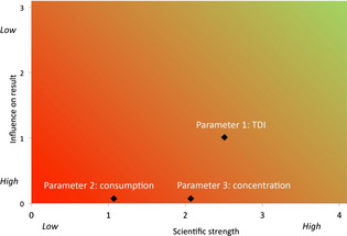
For more details on NUSAP, see Annex B.4.

A.5.5. Uncertainty tables for quantitative questions

Uncertainty tables for quantitative questions list sources of uncertainty affecting the assessment together with expert judgements of their individual and combined impacts on the assessment conclusion, using plus and minus symbols to indicate the direction and magnitude of the impacts.

Short summary of contribution to uncertainty analysis: ‘The worst case exposure is estimated at 269% of the TDI but could lie below 30% or up to 1300%’. This should be accompanied by the same caveat as in EFSA (2008): that it is unknown whether the exposure scenario occurs (Contribution to output of uncertainty analysis).

This is based on expert judgement of uncertainties affecting three inputs to the assessment and their impact on the assessment conclusion, using a defined scale of symbols, followed by conversion of the symbols for the output to quantitative estimates using the same scale.

Parameters		Value in EFSA (2008) assessment	Uncertainty range
Assessment inputs	TDI	0.5 mg/kg bw per day	−−−/++a
	Highest concentration of melamine in milk powder	2,563 mg/kg	−−−/+
	Highest consumption of Chinese chocolate by children	0.044 kg	−−−/++
Assessment output	Ratio of the calculated exposure to the TDI	269%	−−−−/++a (< 30–1,300%)

^aOne expert considered these uncertainties to be unquantifiable.

Scale for ranges shown in the table above (note scale is multiplicative as indicated by ‘x’):

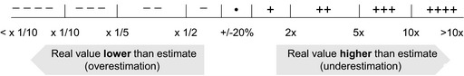
For more details on uncertainty tables for quantitative questions, see Annex B.5.

A.5.6. Uncertainty table for questions

This method provides a structured approach for addressing uncertainty in weight of evidence assessment of categorical questions and expressing the uncertainty of the conclusion.

For the melamine case, it was applied to the question: does melamine have the capability to cause adverse effects on kidney in humans?

Short summary of contribution to uncertainty analysis: ‘It is Very likely (90–100% probability) that melamine has the capability to cause adverse effects on kidney in humans’ (Contribution to output of uncertainty analysis).

This is based on four lines of evidence, as shown in the table below. Expert judgement was used to assess the influence of each line of evidence on the conclusion to the question, expressed using arrow symbols and the probability of a positive conclusion.

Lines of evidence	Influence on conclusiona
Line of Evidence 1 – animal studies	↑↑↑
Line of Evidence 2 – information on effects in humans	↑/↑↑
Line of Evidence 3 – information on mode of action	↑/↑↑
Line of Evidence 4 – evidence of adverse effects in companion animals	↑/↑↑
CONCLUSION on whether melamine has the capability to cause adverse effects on kidney in humans	Very likely (90–100% probability)

^aKey to symbols: ↑, ↑↑, ↑↑↑ represent minor, intermediate and strong upward influence on probability, respectively. Pairs of symbols (↑/↑↑) represent variation of judgements between assessors.

For more details on uncertainty tables for categorical questions, see Annex B.6.

A.5.7. Interval analysis

Interval analysis is a method to compute a range of values for the output of a calculation or quantitative model based on specified ranges for the individual inputs. The output range includes all values which could be obtained from the calculation by selecting a single value from the specified range for each input.

Short summary of contribution to uncertainty analysis: ‘The worst case exposure is estimated to lie between 11 and 66 times the TDI’ (Contribution to output of uncertainty analysis).

This was derived by interval analysis from minimum and maximum possible values for each input to the calculation, specified by expert judgement, as shown in the table below.

Parameters		Minimum possible value	Maximum possible value
Inputs	Maximum concentration (mg/kg) of melamine in milk powder	2,563	6,100
	Maximum fraction, by weight, of milk powder in milk chocolate	0.28	0.30
	Maximum consumption (kg/day) of milk chocolate in a single day by a child aged from 1 up to 2 years	0.05	0.1
	Minimum body weight (kg) of child aged from 1 up to 2 years	5.5	6.5
Outputs	Maximum intake (mg/kg bw per day) of melamine in a single day, via consumption of milk chocolate, by a child aged from 1 up to 2 years	5.5	33.3
	Ratio of maximum intake to TDI for melamine	11	66.6

For more details on interval analysis, see Annex B.7.

A.5.8. Expert Knowledge Elicitation (formal and semi‐formal)

Expert knowledge elicitation (EKE) is a collection of methods for quantification of expert judgements of uncertainty, about an assessment input or output, using subjective probability.

Short summary of contribution to uncertainty analysis: A distribution for use in probabilistic calculations, representing expert judgement about the uncertainty of the maximum fraction of milk powder used in making milk chocolate (Input to uncertainty analysis).

For the purpose of the case study, an illustrative example was constructed, comprising judgements of three fictional experts for minimum, maximum and quartiles, from which the following aggregate distribution was derived (n.b. the vertical axis is probability density).

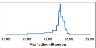
For more details on formal and semi‐formal EKE, see Annex B.8 and B.9.

A.5.9. Statistical Inference from Data

Each of the methods in this section addresses uncertainty about the parameters of a statistical model for variability based on data. Examples are given in relation to (i) variability of (base 10) logarithm of body weight and (ii) variability of consumption of chocolate for children aged from 1 up to 2 years.

Confidence Intervals

Confidence intervals representing uncertainty about the parameters for a statistical model describing variability are estimated from data. The result is a range of values for each parameter having a specified level of confidence.

Short summary of contribution to uncertainty analysis: 95% confidence intervals representing uncertainty due to sampling variability for the geometric mean and standard deviation of body weight were (10.67, 11.12) and (1.13, 1.17) respectively (Input to uncertainty analysis).

This was calculated from the observed mean and standard deviation of a sample of body weights, assuming they were a random sample from a lognormal distribution.

For more details on confidence intervals, see Annex B.10.

The Bootstrap

The bootstrap is a method for obtaining an approximation of uncertainty for one or more estimates, in the form of a sample of possible values, by resampling data to create a number of hypothetical data sets of the same size as the original one.

Short summary of contribution to uncertainty analysis: A bootstrap sample of values for mean and standard deviation of log body‐weight distribution, as an approximate representation of uncertainty due to sampling for use in probabilistic calculations (Input to uncertainty analysis).

The means (μ_logbw) and standard deviations (σ_logbw) for log body weight in the original data and 999 bootstrap samples are plotted in the following Figure.

For more details on the bootstrap, see Annex B.11.

Bayesian Inference

Bayesian inference is a method for quantifying uncertainty about parameters in a statistical model of variability on the basis of data and expert judgements about the values of the parameters.

Short summary of contribution to uncertainty analysis: Distributions quantifying uncertainty due to sampling variability about the mean and standard deviation of log body weight, suitable for use in probabilistic calculations (Input to uncertainty analysis).

The distributions for the uncertainty of the standard deviation (σ_logbw) and mean (μ_logbw) of log body weight are plotted in the following Figures. The distribution for the mean is conditional on the standard deviation as indicated by the values on the horizontal axis, which are functions of σ).

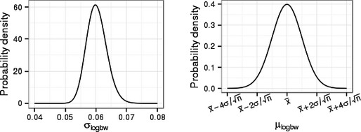
For more details on Bayesian inference, see Annex B.12.

A.5.10. Probability bounds analysis

Probability bounds analysis is general method for combining partial probability statements (i.e. not complete probability distributions) about inputs in order to make a partial probability statement about the output of a calculation or quantitative model.

Short summary of contribution to uncertainty analysis: ‘There is at most a 10% chance that the worst case exposure exceeds 37 times the TDI’ (Contribution to output of uncertainty analysis).

This is one of the outputs produced by probability bounds analysis, shown in the Table below. Also shown are the partial probability statements for each input to the calculation, which were specified by expert judgement.

Parameters		Threshold value	Probability parameter exceeds threshold value
Inputs	Maximum concentration (mg/kg) of melamine in milk powder	3,750	≤ 3.5%
	Maximum fraction, by weight, of milk powder in milk chocolate	0.295	≤ 2%
	Maximum consumption (kg/day) of milk chocolate in a single day by a child aged from 1 up to 2 years	0.095	≤ 2.5%
	Minimum body weight (kg) of child aged from 1 up to 2 years	1/(5.6)	≤ 2%
Outputs	Maximum intake (mg/kg bw per day) of melamine in a single day, via consumption of milk chocolate, by a child aged from 1 to 2 years	18.6	≤ 10%
	Ratio of maximum intake to TDI for melamine	37.2	≤ 10%

For more details on probability bounds analysis, see Annex B.13.

A.5.11. 1D Monte Carlo (uncertainty only)

One‐dimensional (1D) Monte Carlo simulation can be used for combining uncertainty about several inputs to a calculation or quantitative model by numerical simulation when analytical solutions are not available.

Short summary of contribution to uncertainty analysis: ‘There is a 95% chance that the worst case exposure lies between 14 and 30 times the TDI, with the most likely values lying towards the middle of this range’ (Contribution to output of uncertainty analysis).

This is based on a distribution for the uncertainty of the worst‐case exposure (e_max) produced by 1D Monte Carlo, shown in the following figure, calculated by sampling from distributions for the exposure parameters and the TDI of 0.5 mg/kg bw per day.

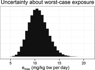
For more details on Monte Carlo for uncertainty only, see Annex B.14.

A.5.12. 2D Monte Carlo (uncertainty and variability)

Two‐dimensional (2D) Monte Carlo simulation separates distributions representing uncertainty from distributions representing variability and provides an uncertainty distribution for any interesting summary of variability, in this case the percentage of 1–2 years old children exceeding the TDI.

Short summary of contribution to uncertainty analysis: ‘The majority of 1 year old children consuming chocolate from China contaminated with melamine will be exposed to levels well below the TDI. There is a 95% chance that the percentage of 1–2 year old children exceeding the TDI is between 0.4% and 5.5%, with the most likely values lying towards the middle of this range’ (Contribution to output of uncertainty analysis).

This is based on a 2D distribution quantifying variability and uncertainty of exposure for 1–2 years old children produced by 2D Monte Carlo, shown in the following figure, based on 2D distributions for the exposure parameters and the TDI of 0.5 mg/kg bw per day. The horizontal axis is the ratio (r) of exposure to the TDI. The vertical line shows where exposure equals the TDI (r = 1), the light grey band corresponds to 95% uncertainty range, and dark grey band corresponds to 50% uncertainty range.

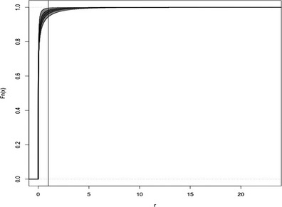
For more details on Monte Carlo for uncertainty and variability, see Annex B.14.

A.5.13. Deterministic calculations with conservative assumptions

These methods deal with uncertainty by using deterministic calculations with assumptions that are conservative, in the sense of tending to overestimate risk.

Short summary of contribution to uncertainty analysis: ‘The highest estimate of adult exposure was 120% of the TDI, while for children consuming both biscuits and chocolate could potentially exceed the TDI by more than threefold’ (Contribution to output of uncertainty analysis).

For more details, see Annex B.16.

A.5.14. Sensitivity analysis

Sensitivity analysis is a suite of methods for assessing the sensitivity of the output of a calculation or quantitative model to the inputs and to choices made expressing uncertainty about inputs.

Short summary of contribution to uncertainty analysis: ‘Exposure is most sensitive to variations in melamine concentration and to a lesser extent chocolate consumption’ (Contribution to output of uncertainty analysis).

This is based on outputs from several methods of sensitivity analysis for the melamine example, two of which are shown below. For both the nominal range sensitivity analysis index and Sobol first‐order index, larger values indicated parameters with more influence on the exposure estimate: melamine concentration and chocolate consumption are more influential than milk powder fraction or body weight which hardly affects the model results.

Input parameters	Nominal range sensitivity analysis index	Sobol first‐order index
Concentration (mg/kg) of melamine in milk powder	1.38	0.54
Fraction, by weight, of milk powder in milk chocolate	0.07	0.01
Consumption (kg/day) of milk chocolate in a single day by a child aged from 1 up to 2 years	1	0.19
Body weight (kg) of child aged from 1 up to 2 years	0.17	0.00

For more details on sensitivity analysis, see Annex B.17.

Annex B – Qualitative and quantitative methods to assess uncertainty

1.

The individual methods are reviewed in detail in the following sections, as shown in the list below:

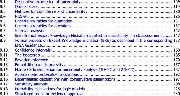
B.1. Descriptive expression of uncertainty

Purpose, origin and principal features

Descriptive expression of uncertainty in this document refers to a form of qualitative assessment of uncertainty using verbal expressions only, without any defined ordinal scale, and without any quantitative definitions of the words. It originates in everyday language rather than any formulated system or theory of uncertainty analysis.

Verbal descriptions are important for expressing the nature or causes of uncertainty. They may also be used to describe the magnitude of an individual uncertainty, the impact of an individual uncertainty on the assessment conclusion or the collective impact of multiple sources of uncertainty on the assessment conclusion.

Descriptive expression of uncertainty may be explicit or implicit. Explicit descriptions refer directly to the presence, magnitude or impact of the uncertainty, for example, ‘the estimate of exposure is highly uncertain’. In implicit descriptions, the uncertainty is not directly expressed but instead implied by the use of words such as ‘may’, ‘possible’ or ‘unlikely’ that qualify, weaken or strengthen statements about data or conclusions in a scientific assessment, for example, ‘it is unlikely that the exposure exceeds the ADI’.

Descriptive information on uncertainty may be presented at different points within a scientific assessment, Report or Opinion. Individual sources of uncertainty may be described at the specific points of the assessment, where they arise. They may also be summarised and/or discussed together, as part of sections that discuss or interpret the assessment. In some cases, the assessment may include a separate section that is specifically identified as dealing with uncertainty.

Applicability in areas relevant for EFSA

Descriptive phrases are the most commonly used method for expressing uncertainty in scientific assessment, by EFSA as well as other authorities. In documents produced by EFSA's Panels, such phrases are produced through an iterative drafting process in a Working Group and in its parent Panel or Scientific Committee. At each stage of this process, phrases that are regarded as important or controversial may attract detailed discussion. The Opinion is finalised and adopted by consensus of the Panel or Scientific Committee. If no consensus can be reached then the minority view(s) are recorded in the Opinion, although this is uncommon (about 14 instances up to October 2014).

In order to inform the development of an Opinion on risk assessment terminology (EFSA, 2012), EFSA commissioned a review by external contractors of the language used in the concluding and summary sections of 219 EFSA Opinions published between 2008 and the beginning of 2010. The review found 1,199 descriptors which were interpreted by the review authors as expressing uncertainty, of which 1,133 were qualitative and 66 quantitative (Table 4 in FERA, 2010). Separate sections dedicated to a type of uncertainty analysis were included in 30 of the 219 documents reviewed.

EFSA's guidance on transparency (EFSA, 2009) states that uncertainties and their relative importance and influence on the assessment conclusion must be described. The Opinion of the EFSA Scientific Committee on risk assessment terminology (EFSA, 2012) recommends the use of defined terminology for risk and uncertainty. The Opinion also notes that some words (e.g. ‘negligible’, ‘concern’ and ‘unlikely’) have risk management connotations in everyday language and recommends that, when used in EFSA Opinions, they should be used carefully with objective scientific definitions so as to avoid the impression that assessors are making risk management judgements.

Selected examples from the review by FERA (2010) are presented in Table B.1 to provide an indication of the types of words that were used in different contexts in EFSA Opinions at that time. The five most frequent descriptors in each category are shown, taken from Tables 17.1–17.9 of FERA (2010). The words that were interpreted as the review authors as expressing possibility or probability are all referring to situations of uncertainty, since they all indicate the possibility of different conclusions. Words expressing difficulty of assessment also imply uncertainty (about what the conclusion of the assessment should be), as do words expressing lack of data or evidence. The data presented in the report do not distinguish the use of words to describe uncertainty from their use to describe benefit, efficacy or risk, therefore not all of the words in the Table B.1 refer exclusively to uncertainty. Even so, many of the words are ambiguous, in that they provide a relative description whose absolute magnitude is unspecified (e.g. High, Rare, Increase). Other words convey certainty, e.g. some of those relating to comparisons (e.g. Higher), change (e.g. Exceed), agreement (e.g. Agrees with) and absence (e.g. No/Not, which is the most frequent of all the descriptors reviewed).

Table B.1.

Examples of descriptive terms used in EFSA Opinions

Context as perceived by authors of FERA (2010)	Most frequent descriptors found by FERA (2010). Numbers are frequency of occurrence, out of 3882 descriptors identified in 219 Opinions
Words perceived as expressing possibility or probability	May 104, Potential 92, Unlikely 79, Can 47, Likely 46
Words perceived as expressing difficulty or inability to assess or evaluate	Cannot 34, Not possible 30, Could not 18, Not appropriate 9, No conclusion(s) 7
Words perceived as expressing magnitude of benefit or efficacy or risk and/or uncertainty	High 105, Low 92, Safety concern(s) 78, Limit/Limited 52, Moderate 49
Words perceived as expressing comparison of benefit, efficacy or risk or uncertainty	Higher 48, Below 32, Increase/Increased/Increasing 26, Lower 25, Highest 23
Words perceived as expressing frequency relevant to the assessment of benefit or efficacy or risk or uncertainty	Rare/Rarely 15, Occasional/Occasionally/On occasion 5, Often 5, Usually 5, Most frequently 3
Words perceived as expressing change or noChange	Increase/Increased/Increasing 43, Reduce/Reduced 26, Exceed/Exceeded/Exceeding 10, Not exceed/Not be exceeded 8, No change/Not changed 5
Words perceived as expressing agreement or disagreement usually referring to a previous assessment	Agrees with 8, Concurs with 4, Does not agree 4, Confirm 3, Remain(s) valid 3
Words perceived as driving a definite yes/noConclusion	No/Not 225, Contributes 11, Cause/Caused/Causing 10, Demonstrated 8, Established 8
Words perceived as contributing in the characterisation of benefit or efficacy or riskand/or uncertainty, and did not belong to any of the above defined categories	No indication/Do not indicate 45, Controlled 39, No evidence 20, Associated with 12, No new data/information 9

The table shows the five most frequently found descriptors found in nine different contexts, as perceived by the authors of the FERA (2010) review. Note that several rows of the table refer to benefit, efficacy and risk as well as uncertainty, and the report does not indicate what proportion of occurrences of descriptors relate to each.

The FERA (2010) review considered Opinions published up to early 2010, and therefore, does not indicate to what extent the recommendations of EFSA (2009, 2012a,b,c) have been implemented in EFSA's subsequent work.

Potential contribution to major elements of uncertainty analysis

Potential contribution of descriptive expression to major elements of uncertainty analysis, as assessed by the Scientific Committee.

Elements in uncertainty analysis	Potential contribution of this approach
Identifying uncertainties	Not applicable
Characterising uncertainties	Verbal description
Combining uncertainties	Verbal description
Prioritising uncertainties	Verbal description

Melamine example

Descriptive narrative is the main method that was used to express uncertainties in the EFSA (2008) statement on melamine. The summary of the statement includes the following phrases, in which the words indicating the presence of uncertainty have been italicised:

‘There is uncertainty with respect to the time scale for the development of kidney damage’.

‘In the absence of actual data for milk powder, EFSA used the highest value of melamine…’

‘Children who consume both such biscuits and chocolate could potentially exceed the TDI by more than threefold. However, EFSA noted that it is presently unknown whether such high level exposure scenarios may occur in Europe’.

Many further examples can be identified within the detailed text of the EFSA (2008) statement.

Strengths

1. Intuitive, requires no special skills (for assessors proficient in the language used for the assessment).

2. Flexibility – language can in principle describe any uncertainty.

3. Single uncertainties and overall uncertainty and its rationale can be expressed in a narrative.

4. Requires less time than other approaches, except when the choice of words provokes extensive discussion (sometimes revisited in multiple meetings).

5. Accepted (or at least not challenged) in most contexts by assessors, decision‐makers and stakeholders (but see below).

Weaknesses and possible approaches to reduce them

1. Verbal expressions without quantitative definitions are ambiguous: they are interpreted in different ways by different people. This causes a range of problems, discussed in Section 4.2 of the Guidance Document and by EFSA (2012a,b,c).; These problems were recognised by some risk managers interviewed during the development of this document, who said they would welcome a move to less ambiguous forms of expression. Ambiguity could be reduced and consistency improved by providing precise (if possible, quantitative) definitions.

2. Where descriptive expression refers to the magnitude of uncertainty, ambiguous wording may leave the decision‐makers to assess for themselves the range and probability of conclusions – which is a scientific question that should be addressed by assessors. Again, this can be avoided by providing precise definitions.

3. Some words that are used in situations of uncertainty imply risk management judgements, unless accompanied by objective scientific definitions.

4. Lack of transparency of the basis for conclusions that are presented as following from a combination of considerations involving descriptive expressions of uncertainty; this could be partially addressed by describing the relative weight given to each uncertainty.

5. Lack of repeatability due to incomplete recording of the individual experts’ involvement and of the chain of arguments leading to the expression of risk and the associated uncertainties; this could in principle be addressed by appropriate recording.

Assessment against evaluation criteria

This method is assessed against the criteria in Table B.2

Table B.2.

Assessment of Descriptive expression of uncertainty (when applied well) against evaluation criteria

Criteria	Evidence of current acceptance	Expertise needed to conduct	Time needed	Theoretical basis	Degree/extent of subjectivity	Method of propagation	Treatment of uncertainty and variability	Meaning of output	Transparency and reproducibility	Ease of understanding for non‐specialist
Stronger characteristics	International guidelines or standard scientific method	No specialist knowledge required	Hours	Well established, coherent basis for all aspects	Judgement used only to choose method of analysis	Calculation based on appropriate theory	Different types of uncertainty & variability quantified separately	Range and probability of possible answers	All aspects of process and reasoning fully documented	All aspects fully understandable
	EU level guidelines or widespread in practice	Can be used with guidelines or literature	Days	Most but not all aspects supported by theory	Combination of data and expert judgement	Formal expert judgement	Uncertainty and variability quantified separately	Range and relative possibility of answers	Most aspects of process and reasoning well documented	Outputs and most of process understandable
	National guidelines, or well established in practice or literature	Training course needed	Weeks	Some aspects supported by theory	Expert judgement on defined quantitative scales	Informal expert judgement	Uncertainty and variability distinguished qualitatively	Range of answers but no weighting	Process well documented but limited explanation of reasoning	Outputs and principles of process understandable
	Some publications and/or regulatory practice	Substantial expertise or experience needed	A few months	Limited theoretical basis	Expert judgement on defined ordinal scales	Calculation or matrices without theoretical basis		Quantitative measure of degree of uncertainty	Limited explanation of process and/or basis for conclusions	Outputs understandable but not process
Weaker characteristics	Newly developed	Professional statistician needed	Many months	Pragmatic approach without theoretical basis	Verbal description, no defined scale	No propagation	No distinction between variability and uncertainty	Ordinal scale or narrative description for degree of uncertainty	No explanation of process or basis for conclusions	Process and outputs only understandable for specialists

Conclusions

1. Descriptive expression is currently the main approach to characterising uncertainty in EFSA and elsewhere. However, there are reasons to move towards more quantitative forms of expression, (see EFSA 2012 and Section 4 of Guidance Document).

2. When a descriptive expression of uncertainty is used, the inherent ambiguity of language means that care is needed to avoid misinterpretation. Ambiguity can be reduced by providing precise definitions that are consistently used across Panels, and by increased dialogue between assessors and decision‐makers.

3. When uncertainty is quantified, it may be useful to accompany it with descriptive expression, as the intuitive nature and general acceptance of descriptive expression make it a useful part of the overall communication.

4. Special care is required to avoid using language that implies value judgements, unless accompanied by objective scientific definitions.

5. Descriptive expression should be used to communicate the nature and causes of uncertainty. This is especially important for any uncertainties that are not included in the quantitative assessment (see Sections 5.12, 5.13 and 14).

References

EFSA, 2009. Guidance of the Scientific Committee on transparency in the scientific aspects of risk assessment carried out by EFSA. Part 2: general principles. The EFSA Journal (2009) 1051, 1–22.

EFSA, 2012. Scientific Opinion on Risk Assessment Terminology. EFSA Journal 2012;10(5):2664.

FERA (Food and Environmental Research Agency, UK), 2010. Flari and Wilkinson: Terminology in risk assessment used by the scientific panels and scientific committee of EFSA. http://www.efsa.europa.eu/en/supporting/pub/101e.htm

B.2. Ordinal scale

B.2.1.

B.2.1.1.

Purpose, origin and principal features

An ordinal scale is one that comprises two or more categories in a specified order without specifying anything about the degree of difference between the categories. For example, an ordinal scale of low – medium – high has a clear order, but does not specify the magnitude of the differences between the categories (e.g. whether moving from low to medium is the same as moving from medium to high). Ordinal scales provide more information than nominal scales (descriptive categories with no specified order), but less than interval and ratio scales, which quantify the distance between different values (Stevens, 1946). Ordinal scales may therefore be useful when the purpose is to describe the degree of uncertainty in relative terms, e.g. low, medium or high, but should be accompanied by quantitative expressions of uncertainty when possible.

Numerical values can be assigned to the categories as labels, but should then not be interpreted as representing the magnitude of differences between categories. Ordinal scales can be used to rank a set of elements, e.g. from lowest to highest; either with or without ties (i.e. some elements may have the same rank).

Ordinal scales can be used to describe the degree of uncertainty in a qualitative or quantitative risk assessment, e.g. low uncertainty, medium uncertainty. Clearly, it is desirable to provide a definition for each category, so that they can be used and interpreted in a consistent manner. In many cases, including the examples provided in the following section, the definitions refer to the causes of uncertainty (e.g. amount, quality and consistency of evidence, degree of agreement amongst experts). Strictly speaking, these are scales for the amount and quality of evidence rather than degree of uncertainty, although they are related to the degree of uncertainty: e.g. limited, poor quality evidence is likely to lead to larger uncertainty. This relationship is reflected in the approach used by IPCC (Mastrandrea et al., 2010), where 3‐point scales for ‘Evidence (type, amount, quality, consistency)’ and ‘Agreement’ are combined to derive the ‘Level of confidence’, which is assessed on a 5‐point scale from ‘very low’ to ‘very high’. Level of confidence is inversely related to degree of uncertainty, as discussed in Section 5.8.

Ordinal scales for degree of uncertainty should ideally represent the magnitude of uncertainty, e.g. the degree to which the true value of a parameter could differ from its estimate. This could be expressed ordinally with categories such as low, medium, high. However, it will usually be important also to provide information on the direction of the uncertainty, e.g. whether the true value is more likely to be higher or lower than the estimate. Perhaps the simplest way to represent this with ordinal scales would be to use a pair of ordinal scales, one indicating how much lower the true value could be, and the other indicating how much higher it could be. An example of this is the +/− scale suggested by EFSA (2006, 2007), described in the following section. For categorical questions of interest (e.g. whether an effect observed in animals can also occur in humans), uncertainty could be expressed on an ordinal scale for probability (ideally with quantitative definitions, e.g. Mastrandrea et al., 2010).

Applicability in areas relevant for EFSA

Some EFSA Panels have used ordinal scales that are described as scales for uncertainty, but defined in terms of evidence (e.g. type, amount, quality, consistency) and the level of agreement between experts. In a joint opinion in 2010, the Animal Health and Animal Welfare Panel (AHAW) and the BIOHAZ Panel defined three levels of uncertainty associated with the assessment of the effectiveness of different disease control options of Coxiella burnetii, the causative agent of Q‐fever (EFSA, 2010a,b).

• ‘Low: Solid and complete data available; strong evidence in multiple references with most authors coming to the same conclusions, or considerable and consistent experience from field observations’.

• ‘Medium: Some or only incomplete data available; evidence provided in small number of references; authors’ or experts’ conclusions vary, or limited evidence from field observations, or solid and complete data available from other species which can be extrapolated to the species being considered’.

• ‘High: Scarce or no data available; evidence provided in unpublished reports, or few observations and personal communications, and/or authors’/or experts’ conclusions vary considerably’.

As can be seen in this example, different emphasis may be given to the different descriptors used in the definitions: some to the availability of data or the strength of evidence provided; and some to the level of agreement, either in the published literature or in expert's opinions.

The Plant Health (PLH) Panel uses ordinal scales for assessing both risk and uncertainty. Risk assessments are considered in sequential components: entry, establishment, spread and impact of the harmful organism. For each of these components, there may be multiple pathways to consider. At each stage of the assessment, risk ratings are made on a 5‐category ordinal scale (e.g. very unlikely – unlikely – moderately likely – likely – very likely), where the descriptors for the categories must be specified and justified in advance. For each rating, a rating of the associated uncertainty (i.e. the level of confidence in the risk rating given) must also be made. Hence, for the risk assessment components – entry, establishment, spread and impact – the level of uncertainty has to be rated separately, usually on a 3‐category scale with prespecified definitions similar to those in the AHAW/BIOHAZ example above. An example of this approach is provided by the Opinion on the plant pest and virus vector Bemisia (EFSA, 2013). For plants‐for‐planting, the risk of entry of Bemisia was rated as likely, for cut flowers and branches moderately likely, and for fruits and vegetables unlikely. The uncertainty of each risk rating was assessed on a 3‐point scale (low, medium and high, defined in terms of quality of evidence and degree of subjective judgement) and then consolidated across the three pathways by expert judgement to give a combined uncertainty of ‘medium’ for entry of Bemisia into the EU. This was accompanied by a narrative justification, summarising the rationale for the assessment of ‘medium’ uncertainty.

Ordinal scales defined in terms of the magnitude and direction of uncertainty, rather than amount or quality of evidence, have been used with ‘uncertainty tables’ in some EFSA opinions. The categories in these scales are often represented by different numbers of plus and minus symbols, e.g. +, ++, +++. Early examples provided qualitative definitions for the categories such as small, medium or large over‐estimation of exposure (EFSA, 2006) and are therefore ordinal scales. Some later examples define the symbols by mapping them on to a quantitative scale, as in the exposure assessment for bisphenol A (EFSA, 2015). This makes the meaning of the categories less ambiguous, and opens the possibility of converting them to intervals for use in quantitative calculations (interval analysis or sensitivity analysis, see Sections B.1 and B.2). However, since a scale of such categories is no longer strictly ordinal, they are not further discussed here (see instead Annex B.3).

Potential contribution to major elements of uncertainty analysis

Potential contribution of ordinal scales to major elements of uncertainty analysis, as assessed by the Scientific Committee.

Elements in uncertainty analysis	Potential contribution of this approach
Identifying uncertainties	Not applicable
Characterising uncertainties	Provides an ordered set of descriptors for expressing magnitude of uncertainty or level of confidence. Can also be used to describe factors that contribute to uncertainty, e.g. the type, amount, quality and consistency of evidence, or the degree of agreement. Categories defined in terms of evidence or agreement may provide indirect measures of magnitude of uncertainty. Assignation of individual uncertainties to the defined categories is assessed by expert judgement.
Combining uncertainties	Ordinal scales can be used to express expert judgements about the combined impact of multiple uncertainties on the assessment output, but provide a more limited expression than quantitative judgements. No theoretically justified methods available for propagating ordinal categories with qualitative definitions.
Prioritising uncertainties	Can be used to rank uncertainties on the ordinal scale that is used. Also, may inform expert judgement of relative contributions to overall uncertainty.

Melamine example

Members of the Working Group applied an ordinal scale to assess three uncertainties affecting the example assessment of melamine. They considered uncertainty of the answer to the following question: does the possible worst‐case exposure of high‐consuming European children to melamine from consumption of chocolate containing contaminated Chinese milk powder exceed the relevant health‐based guidance value, and if so by how much?

The group first defined an ordinal scale for use in the example, based on the 3‐level scale with qualitative definitions in terms of level of evidence and agreement that is shown earlier in this section. The group expanded this to a 4‐point scale, on the grounds that this avoids a potential tendency for assessors to pick the central category. For the purpose of illustration, the group retained wording similar to that of the original categories. The four categories used for the example were as follows:

• Low uncertainty (L): Solid and complete data available; strong evidence in multiple references with most authors coming to the same conclusions, or considerable and consistent experience from field observations.

• Low to medium uncertainty (LM): Moderate amount of data available; evidence provided in moderate number of references; moderate agreement between authors or experts, or moderate evidence from field observations, or solid and complete data available from other species which can be extrapolated to the species being considered.

• Medium to high uncertainty (MH): Some or only incomplete data available; evidence provided in small number of references; authors’ or experts’ conclusions vary, or limited evidence from field observations, or moderate data available from other species which can be extrapolated to the species being considered.

• High uncertainty (H): Scarce or no data available; evidence provided in unpublished (unverified) reports, or few observations and personal communications, and/or authors’/or experts’ conclusions vary considerably.

The group members were asked to use the above scale to assess three selected sources of uncertainty (content of melamine in milk powder, Chinese chocolate consumption of European children and appropriate health guidance value for melamine), by expert judgement, and also to assess the combined impact of these three sources of uncertainty on the uncertainty of the assessment conclusion. The evaluation was conducted in two rounds, with the scores from the first round being collated on‐screen and discussed before the second round. This allowed assessors to adjust their scores in the light of the discussion, if they wished. The results are shown in Table B.3. If it was desired to arrive at a ‘group’ evaluation of uncertainty, this could be done either by seeking a consensus view by discussion, or by ‘enveloping’ the range of categories assigned for each source of uncertainty in the second round. In this example, the latter option would result in evaluations of LM/MH, MH and MH/H for the three individual sources of uncertainty and MH for the combined uncertainty in the second round.

Table B.3.

Example of the use of an ordinal scale (defined in the text above) to evaluate three sources of uncertainty affecting the melamine example assessment

Assessor	Hazard characterisation (TDI)	Concentration of melamine in milk powder	Consumption of Chinese chocolate	Combined
1	LM/LM	MH/MH	H/MH	MH/MH
2	LM/LM	MH/MH	H/H	MH/MH
3	MH/LM	LM/MH	MH/MH	MH/MH
4	H/MH	LM/MH	MH/MH	MH/MH
5	H/MH	H/MH	MH/MH	MH/MH
6	LM/LM	MH/MH	MH/MH	LM/MH
7	MH/LM	MH/MH	MH/H	MH/MH

Pairs of scores (e.g. H/MH) show the first and second rounds of assessment, respectively.

Strengths

1. Guidelines exist and the method is already used by certain EFSA Panels.

2. Structured approach to rating uncertainties which forces assessors to discuss and agree the ratings (what is meant by, e.g. low, medium and high).

3. Ordinal expressions for sources of uncertainty that are not individually quantified may provide a useful summary to inform quantitative expert judgements about the overall uncertainty of the assessment conclusion, and to help document the reasoning behind them.

Weaknesses and possible approaches to reduce them

1. Ordinal categories without definitions or with qualitative definitions are subject to linguistic ambiguity, and will be interpreted in different ways by different people. This can partly be avoided by the use of ordinal categories with quantitative definitions such as the IPCC scale for likelihood (Mastrandrea et al., 2010).

2. Ordinal categories with qualitative definitions are sometimes labelled with numbers rather than words. This increases the chance that they will be interpreted as expressing a quantitative definition of the degree of uncertainty, which is invalid.

3. Statistical approaches are sometimes used to combine and summate numerical ratings of uncertainty made on an ordinal scale (e.g. mean and variance), for different experts or different sources of uncertainty or both, but this is not valid. Use of the mode, median and percentiles may be appropriate, but are better applied to verbal category descriptors (e.g. the modal uncertainty category is ‘high’) to avoid invalid interpretation (see preceding point).

4. Although it is possible to devise rules or calculations for combining ordinal measures of uncertainty or propagating them through an assessment, there is no valid theoretical basis for this.

5. Ordinal scales are often defined in terms of evidence and level of agreement: these are measures of evidence and only an indirect indication of degree of uncertainty. Therefore, interpreting such a scale as a measure of uncertainty is likely to be incomplete and misleading.

6. Ordinal scales defined in terms of confidence are more directly related to uncertainty, but generally lack a clear interpretation in terms of the range and probability of different answers.

7. Use of three categories in an ordinal scale might lead to a bias towards assigning the middle category. This can be avoided by using four categories.

Assessment against evaluation criteria

The use of ordinal scales for evaluating uncertainty is assessed against the Scientific Committee's criteria in Table B.4. The evaluation is based on ordinal scales with qualitative definitions, since a scale with quantitative definitions is no longer ordinal and is closer to an interval approach (see Annex B.1). For some criteria, a range of levels are ticked, as the assessment depends on how ordinal scales are used (with qualitative or quantitative definitions for categories) and where they are applied (to individual uncertainties or overall uncertainty).

Table B.4.

Assessment of Ordinal scales with qualitative definitions for expression of uncertainty (when applied well) against evaluation criteria

Criteria	Evidence of current acceptance	Expertise needed to conduct	Time needed	Theoretical basis	Degree/extent of subjectivity	Method of propagation	Treatment of uncertainty and variability	Meaning of output	Transparency and reproducibility	Ease of understanding for non‐specialist
Stronger characteristics	International guidelines or standard scientific method	No specialist knowledge required	Hours	Well established, coherent basis for all aspects	Judgement used only to choose method of analysis	Calculation based on appropriate theory	Different types of uncertainty & variability quantified separately	Range and probability of possible answers	All aspects of process and reasoning fully documented	All aspects fully understandable
	EU level guidelines or widespread in practice	Can be used with guidelines or literature	Days	Most but not all aspects supported by theory	Combination of data and expert judgement	Formal expert judgement	Uncertainty and variability quantified separately	Range and relative possibility of answers	Most aspects of process and reasoning well documented	Outputs and most of process understandable
	National guidelines, or well established in practice or literature	Training course needed	Weeks	Some aspects supported by theory	Expert judgement on defined quantitative scales	Informal expert judgement	Uncertainty and variability distinguished qualitatively	Range of answers but no weighting	Process well documented but limited explanation of reasoning	Outputs and principles of process understandable
	Some publications and/or regulatory practice	Substantial expertise or experience needed	A few months	Limited theoretical basis	Expert judgement on defined ordinal scales	Calculation or matrices without theoretical basis		Quantitative measure of degree of uncertainty	Limited explanation of process and/or basis for conclusions	Outputs understandable but not process
Weaker characteristics	Newly developed	Professional statistician needed	Many months	Pragmatic approach without theoretical basis	Verbal description, no defined scale	No propagation	No distinction between variability and uncertainty	Ordinal scale or narrative description for degree of uncertainty	No explanation of process or basis for conclusions	Process and outputs only understandable for specialists

Conclusions

1. Ordinal scales are often defined in terms of the nature, amount, quality and consistency of evidence or the degree of agreement between experts. When used in this way, they should be described as scales for evidence or agreement and not as scales for uncertainty, as they do not describe uncertainty directly. However, they may help to inform subsequent judgements about the degree of uncertainty.

2. Ordinal scales can also be used to describe the degree of uncertainty, if they are defined in terms of the range or probability of different answers.

3. Calculations which treat ordinal scales as if they were quantitative are invalid and should not be used.

4. Ordinal scales provide a useful way of summarising multiple sources of uncertainty to inform quantitative judgements about their combined impact, e.g. when assessing the combined effect of uncertainties which are for whatever reason not quantified individually in the assessment.

References

EFSA, 2006. Guidance of the Scientific Committee on a request from EFSA related to Uncertainties in Dietary Exposure Assessment. EFSA Journal 438, 1–54.

EFSA AHAW Panel (EFSA Panel on Animal Health and Welfare), 2010. Scientific Opinion on Q Fever. EFSA Journal 2010;8(5):1595, 114 pp. https://doi.org/10.2903/j.efsa.2010.1595

EFSA PLH Panel (EFSA Panel on Plant Health), 2013. Scientific Opinion on the risks to plant health posed by Bemisia tabaci species complex and viruses it transmits for the EU territory. EFSA Journal 2013;11(4):3162, 302 pp. https://doi.org/10.2903/j.efsa.2013.3162

EFSA CEF Panel (EFSA Panel on Food Contact Materials, Enzymes, Flavourings and Processing Aids), 2015. Scientific Opinion on the risks to public health related to the presence of bisphenol A (BPA) in foodstuffs: Part I – Exposure assessment. EFSA Journal 2015;13(1):3978, 396 pp. https://doi.org/10.2903/j.efsa.2015.3978

Mastrandrea MD, Field CB, Stocker TF, Edenhofer O, Ebi KL, Frame DJ, Held H, Kriegler E, Mach KJ, Matschoss PR, Plattner G‐K, Yohe GW, and Zwiers FW, 2010. Guidance Note for Lead Authors of the IPCC Fifth Assessment Report on Consistent Treatment of Uncertainties. Intergovernmental Panel on Climate Change (IPCC). Available at: http://www.ipcc.ch

Stevens SS, 1946. On the Theory of Scales of Measurement, Science 7 June 1946: 103 (2684), 677–680. https://doi.org/10.1126/science.103.2684.677

B.3. Matrices for confidence and uncertainty

Purpose, origin and principal features

‘Risk matrices’ are widely used as a tool for combining ordinal scales for different aspects of risk (e.g. probability and severity) into an ordinal scale for level of risk. Matrices have also been proposed by a number of authors as a means of combining two or more ordinal scales representing different sources or types of confidence or uncertainty into a third scale representing a combined measure of confidence or uncertainty. The matrix defines what level of the output scale should be assigned for each combination of the two input scales. Ordinal scales themselves are discussed in more detail in Annex B.2; here the focus is on the use of matrices to combine them.

An example of a matrix used to combine two ordinal scales is provided by Figure B.1, used by the Intergovernmental Panel on Climate Change (IPCC, Mastrandrea et al., 2010). The two input scales on the axes of the matrix relate to different sources of confidence in a conclusion: one scale for amount and quality of evidence and the other for degree of agreement (the latter refers to agreement across the scientific community, Kunreuther et al. 2014). These are combined to draw conclusions about the level of confidence in the conclusion. In this example, the relationship between the input and output scales is flexible. IPCC state that, for a given combination of evidence and agreement, different confidence levels could be assigned, but increasing levels of evidence and degrees of agreement are correlated with increasing confidence (Mastrandrea et al., 2010). They also state that level of confidence should be expressed using five qualifiers from ‘very low’ to ‘very high’, synthesising the assessors’ judgements about the validity of findings as determined through evaluation of evidence and agreement. IPCC also state that confidence cannot necessarily be assigned for all combinations of evidence and agreement and, in such cases, the assessors should report only the individual assessments for evidence and agreement.

Searching for ‘uncertainty matrix’ on the internet reveals a substantial number of similar structures from other areas of application.

Applicability in areas relevant for EFSA

The concept of using a matrix to combine ordinal scales representing different sources or types of uncertainty is a general one and could, in principle, be applied to any area of EFSA's work. For example, in an opinion on cattle welfare (EFSA, 2012), the EFSA Animal Health and Welfare Panel expressed the degree of uncertainty in their assessments of exposure and probability using two ordinal scales, and then used a matrix to derive a third ordinal scale for the uncertainty of the resulting risk (Figure B.2).

Figure B.2.

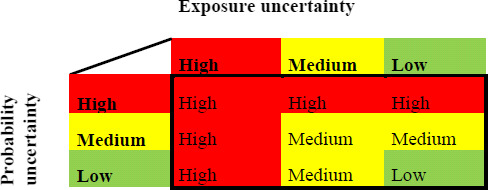
Example of matrix used for combining two ordinal scales representing uncertainty. In this example, the two input scales represent uncertainty in different parts of the uncertainty analysis (uncertainty about exposure to welfare hazards, and uncertainty about the probability of adverse effects given that exposure occurs) and their combination expresses the uncertainty of the assessment as a whole

Potential contribution to major elements of uncertainty analysis

Elements in uncertainty analysis	Potential contribution of this approach
Identifying uncertainties	Not applicable
Characterising uncertainties	Not applicable
Combining uncertainties	Can be used to combine ordinal scales for uncertainty in different parts of an uncertainty analysis, the output expresses the uncertainty of the overall assessment, but cumbersome for more than two sources and lacks a theoretical basis (see below).
Prioritising uncertainties	The matrix shows how the uncertainties represented by the input scales contribute to the combined uncertainty represented by the output scale, but does not identify individual contributions within each input.

Melamine example

The use of an confidence matrix is illustrated here using a modified version of the IPCC matrix (Mastrandrea et al., 2010), in which each of the two input scales has been expanded from 3 to 4 ordinal categories (Table B.5). Note that, as discussed in Section 5.6 of the main text and in Annex B.2 of this annex on ordinal scales, confidence is only a partial measure of uncertainty: it expresses the probability of a specified answer but provides no information on the range or probabilities of alternative answers.

Table B.5.

Confidence matrix combining ordinal scales for evidence and agreement, adapted from Mastrandrea et al. (2010)

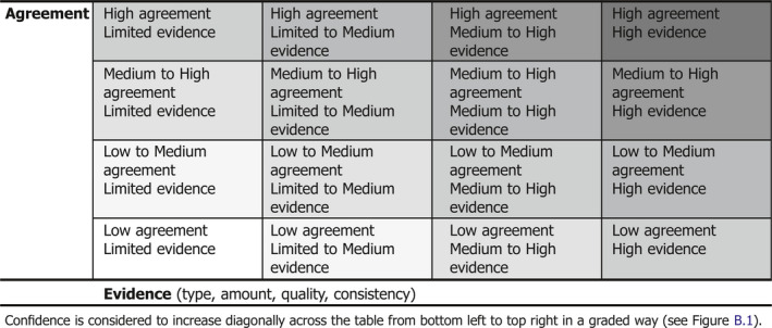
The example considers the uncertainty of the ratio between the worst‐case exposure of the European children from contaminated chocolate and the TDI for melamine, as assessed in the EFSA (2008) melamine statement where the reported estimate was 269%. For the example, six assessors were asked to evaluate the levels Evidence and Agreement supporting the estimate of 269% and then combine these using Table B.5 to assess level of Confidence on the following scale: ‘very low,’ ‘low,’ ‘low to medium,’, ‘medium to high’, ‘high,’ ‘very high’. In doing this, they were invited to make use of the assessment they had conducted immediately previously using a four‐category ordinal scale reported in Annex B.2, where the categories were defined mainly in terms of evidence and the degree of agreement could be judged from the variation in scores between assessors. The assessors’ judgements were collected and displayed on screen for discussion, after which the assessors were given the opportunity to amend their judgements if they wished. The results are shown in Table B.6. Note that although all the assessors gave identical scores for Evidence and Agreement, their assessments for Confidence varied. This is possible because, as in the IPCC matrix, the group did not assign fixed outputs for each cell in their matrix but, instead, assigned the output by expert judgement informed by the combination of inputs.

Table B.6.

Evaluation of evidence, agreement and confidence for assessment of the ratio between the worst‐case exposure of the European children to melamine in contaminated chocolate and the TDI for melamine

Assessor	Evidence	Agreement	Confidence
1	LM	H	MH
2	LM	H	MH
3	LM	H	MH
4	LM	H	LM
5	LM	H	LM
6	LM	H	MH
Range for 6 assessors	LM	H	LM/MH

Key: LM = Low to medium; MH = Medium to high; H = High.

Strengths

1. Simplicity and ease of use: if the matrix gives defined outputs for each combination of inputs (as in Figure B.2), it can be used as a look‐up table. If the matrix gives flexible outputs for each combination of inputs (as in Figure B.1), the user needs to make judgements about what outputs to assign, but these may be informed and facilitated by the matrix.

2. Using a matrix (of either type) provides structure for the assessment that should increase the consistency of the uncertainty analysis and also its transparency (it is easy for others to see what has been done, although not necessarily the reasons for it).

Figure B.1.

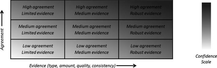
Confidence matrix used by IPCC (Mastrandrea et al., 2010). Confidence increases towards the top‐right corner as suggested by the increasing strength of shading. Generally, evidence is most robust when there are multiple, consistent independent lines of high‐quality evidence

Weaknesses and possible approaches to reduce them

1. Using matrices becomes increasingly cumbersome when more than two inputs are involved.

2. The output of the matrix will only be useful if it has meaning. Bull and Watt. (2013) have demonstrated vastly different evaluations of risk matrices by different individuals and concluded that ‘It appears that risk matrices may be creating no more than an artificial and even untrustworthy picture of the relative importance of hazards, which may be of little or no benefit to those trying to manage risk effectively and rationally’. This requires that unambiguous (preferably quantitative) definitions are provided for the meaning of the output. Ideally, the meaning of each level of the output scale should be defined in terms of its implications for the conclusion of the assessment that is being considered. For example, in the melamine example above, how much higher might the true worst‐case exposure be relative to the relevant health based guidance value, given that confidence in the estimate has been assessed as being in the range ‘Low to medium’ to ‘Medium to high’?

3. Even when the meaning of the output is defined, its reliability will depend on whether the matrix combines the inputs in an appropriate way. Therefore, it is essential that the reasoning for the structure of the matrix should be carefully considered and documented, and take account of the nature and relative importance of the inputs and how they should properly be combined to generate the output. Ideally, it should have an appropriate theoretical basis, e.g. in terms of probability theory. Alternatively, it could be based on subjective judgements about how the inputs combine to produce a meaningful measure of the degree of uncertainty. The latter is likely to be less reliable than the former, because of limitations in human ability to make subjective judgements about probability combinations. The IPCC state that the relation between the inputs and outputs of their matrix is flexible, so the user has to judge it case by case.

4. Superficially, a matrix such as that in Figure B.2 could be applied to any problem, which would be a major strength. However, defining the matrix structure and output scale sufficiently well to have meaning is likely to limit its applicability to the particular problems and uncertainties for which it was designed. The example in Figure B.1 is more generally applicable, but the outputs are not precisely defined and have to be considered by the user, case by case.

5. Even if the matrix structure has a sound basis in probability theory, it will be subject to similar problems to those demonstrated by Cox (2008) for risk matrices. Cox showed that the ordinal input scales discretise the underlying continuous quantities in ways that will cause the matrix outputs to differ, sometimes substantially, from the result that would be obtained by calculation.

6. A matrix does not provide information on the relevant importance of the different sources of uncertainty affecting each of its inputs. If this is needed it should be used in conjunction with other methods.

Assessment against evaluation criteria

The use of uncertainty matrices is assessed against the criteria in Table B.7.

Table B.7.

Assessment of Uncertainty matrices (when applied well) against evaluation criteria

Criteria	Evidence of current acceptance	Expertise needed to conduct	Time needed	Theoretical basis	Degree/extent of subjectivity	Method of propagation	Treatment of uncertainty and variability	Meaning of output	Transparency and reproducibility	Ease of understanding for non‐specialist
Stronger characteristics	International guidelines or standard scientific method	No specialist knowledge required	Hours	Well established, coherent basis for all aspects	Judgement used only to choose method of analysis	Calculation based on appropriate theory	Different types of uncertainty & variability. quantified separately	Range and probability of possible answers	All aspects of process and reasoning fully documented	All aspects fully understandable
	EU level guidelines or widespread in practice	Can be used with guidelines or literature	Days	Most but not all aspects supported by theory	Combination of data and expert judgement	Formal expert judgement	Uncertainty and variability quantified separately	Range and relative possibility of answers	Most aspects of process and reasoning well documented	Outputs and most of process understandable
	National guidelines, or well established in practice or literature	Training course needed	Weeks	Some aspects supported by theory	Expert judgement on defined quantitative scales	Informal expert judgement	Uncertainty and variability distinguished qualitatively	Range of answers but no weighting	Process well documented but limited explanation of reasoning	Outputs and principles of process understandable
	Some publications and/or regulatory practice	Substantial expertise or experience needed	A few months	Limited theoretical basis	Expert judgement on defined ordinal scales	Calculation or matrices without theoretical basis		Quantitative measure of degree of uncertainty	Limited explanation of process and/or basis for conclusions	Outputs understandable but not process
Weaker characteristics	Newly developed	Professional statistician needed	Many months	Pragmatic approach without theoretical basis	Verbal description, no defined scale	No propagation	No distinction between variability and uncertainty	Ordinal scale or narrative description for degree of uncertainty	No explanation of process or basis for conclusions	Process and outputs only understandable for specialists

Conclusions

1. Matrices with ordinal input and output scales that lack quantitative definitions are ambiguous and will be interpreted in different ways by different users.

2. Matrices that specify a fixed relation between input and output should not be used unless a clear justification, based on theory or expert judgement, can be provided for the relationships involved.

3. Matrices that do not specify a fixed relation between input and output might be regarded as a guide for expert judgement, reminding the user of the factors that should be considered when making judgements. However, users may be tempted to apply them as if they represented fixed rules, leading to inappropriate conclusions.

4. Even when the above issues are avoided, matrices become cumbersome when more than two sources or aspects of uncertainty are involved, which is usual in EFSA assessment.

The issues in (1–4) above are likely to limit the usefulness of matrices as a tool for assessing uncertainty in EFSA's work.

References

Ball DJ and Watt J, 2013. Further thoughts on the utility of risk matrices. Risk Anal. 33(11):2068‐78.

Cox LA Jr, 2008. What's wrong with risk matrices? Risk analysis 28, 497–511.

FSA, 2012. Scientific Opinion on the welfare of cattle kept for beef production and the welfare in intensive calf farming systems. The EFSA Journal, 10(5):2669.

Kunreuther H, Gupta S, Bosetti V, Cooke R, Dutt V, Ha‐Duong M, Held H, Llanes‐Regueiro J, Patt A, Shittu E, and Weber E, 2014: Integrated Risk and Uncertainty analysis of Climate Change Response Policies. In: Climate Change 2014: Mitigation of Climate Change. Contribution of Working Group III to the Fifth Assessment Report of the Intergovernmental Panel on Climate Change [Edenhofer, O., R. Pichs‐Madruga, Y. Sokona, E. Farahani, S. Kadner, K. Seyboth, A. Adler, I. Baum, S. Brunner, P. Eickemeier, B. Kriemann, J. Savolainen, S. Schlömer, C. von Stechow, T. Zwickel and J.C. Minx (eds.)]. Cambridge University Press, Cambridge, United Kingdom and New York, NY, USA.

Mastrandrea MD, Field CB, Stocker TF, Edenhofer O, Ebi KL, Frame DJ, Held H, Kriegler E, Mach KJ, Matschoss PR, Plattner G‐K, Yohe GW, and Zwiers FW, 2010. Guidance Note for Lead Authors of the IPCC Fifth Assessment Report on Consistent Treatment of Uncertainties. Intergovernmental Panel on Climate Change (IPCC). Available at http://www.ipcc.ch.

B.4. NUSAP

Purpose, origin and principal features

The purpose of this method is to provide a structured approach to deal with uncertainties in model‐based health risk assessments. The NUSAP acronym stands for: Numeral, Unit, Spread, Assessment and Pedigree. The first three dimensions are related to commonly applied quantitative approaches to uncertainty, expressed in numbers (N) with appropriate units (U) and a measure of spread (S) such as a range or standard deviation. Methods to address spread include statistical methods, sensitivity analysis and expert elicitation. The last two dimensions are specific to NUSAP and are related to aspects of uncertainty than can less readily be analysed by quantitative methods. Assessment (A) expresses qualitative expert judgements about the quality of the information used in the model by applying a Pedigree (P) matrix, implying a multicriteria evaluation of the process by which the information was produced.

The method was first proposed by Funtowicz and Ravetz (1993) and further developed by van der Sluijs et al. (2005) to evaluate the knowledge base in model‐based assessment and foresight studies of complex environmental problems. Such assessments are often characterised by uncertainties in the knowledge base, differences in framing the problem, and high stakes involved in decisions based on these assessments, often with conflicting views between different stakeholders.

The principal features of this method are to consider the background history by which the information was produced, in combination with the underpinning and scientific status of the information. Qualitative judgements about uncertainties are supported by so‐called pedigree matrices, which are then translated in a numerical, ordinal scale. Typically, a pedigree matrix has four dimensions for assessing the strength of parameters or assumptions, and one dimension for their influence on results (e.g. Table B.8).

Table B.8.

Example of NUSAP pedigree matrix for scoring parameter strength and influence

	Strength				Effect
Score	Proxy	Empirical basis	Methodological rigor	Validation	Influence on results
4	Exact measure of the desired quantity (e.g. from the same geographical area)	Large sample, direct measurements (recent data, controlled experiments)	Best available practice (accredited method for sampling/diagnostic test)	Compared with independent measurements of the same variable (long domain, rigorous correction of errors)
3	Good fit or measure (e.g. from another but representative area)	Small sample, direct measurements (less recent data, uncontrolled experiments, low non‐response)	Reliable method (common within established discipline)	Compared with independent measurements of closely related variable (shorter time periods)	No or negligible impact on the results
2	Well correlated (e.g. large geographical differences, less representative)	Very small sample, modelled/derived data (indirect measurements, structured expert opinion)	Acceptable method (limited consensus on reliability)	Compared with measurements of non‐independent variable (proxy variable, limited domain)	Little impact on the results
1	Weak correlation (e.g. very large geographical differences, low representativity)	One expert opinion, rule of thumb	Preliminary method (unknown reliability)	Weak, indirect validation	Moderate impact on the end result
0	Not clearly correlated	Crude speculation	No discernible rigor	No validation	Important impact on the end result

The NUSAP output is a score per uncertainty source for the scientific strength of the information and its influence on the model output. In NUSAP, scientific strength expresses the methodological and epistemological limitations of the underlying knowledge base (van der Sluijs et al., 2005). In comparison to using single ordinal scales, the multicriteria evaluation provides a more detailed and formalised description of uncertainty. The median scores over all experts for the strength and influence are combined for all uncertainty sources in a diagnostic diagram, which will help to identify the key uncertainties in the assessment, i.e. those sources with a low strength and a large influence on the model output. The NUSAP approach therefore can be used to evaluate uncertainties that cannot be quantified, but can also be useful in identifying the most important uncertainties for further quantitative evaluation and/or additional work to strengthen the evidence base of the assessment. Pedigree matrices have been developed to evaluate model parameters and input data as well as assumptions. The method is flexible, in that customised scales can be developed.

The NUSAP method is typically applied in a workshop involving multiple experts with various backgrounds in the subject matter of the assessment. The workshop would build on previous efforts to identify and characterise uncertainties using an appropriate typology. An introductory session would include presentations on the NUSAP methodology, the risk assessment to be evaluated and an open discussion about the identified uncertainties, followed by an introduction to the evaluation methodology and a discussion about the scoring methods. For each assumption, all experts would then be asked to write down their scores on a score‐card and to also describe their rationale. Scores and rationales are then reported by all experts to the group and are the basis for a discussion. Experts are then given the opportunity to adjust their scores and invited to submit their results. Computer‐assisted tools may help to show the key findings of the workshop directly after completing scoring of all uncertainties. The group discussions and iterative process are an important characteristic of the NUSAP process that helps to create a better and collective understanding of uncertainties. However, the method can also be applied by a small number of experts, see e.g. Bouwknegt et al. (2014) in which only two experts provided scores. Data analysis after the workshop involves developing diagnostic diagrams and possibly other data analysis. Also in this respect, the method is flexible and can be adapted to the needs of the risk assessment body.

Applicability in areas relevant for EFSA

The NUSAP methodology has been developed mainly in the environmental sciences, including environmental health risk assessments but is in principle applicable in of EFSA's work. Published examples include an assessment of uncertainties in a Quantitative Microbial Risk Assessment (QMRA) models for Salmonella in the pork chain (Boone et al., 2009) and comparing QMRA‐based and epidemiologic estimates of campylobacteriosis in the Netherlands (Bouwknegt et al., 2014). The method has also been applied in two outsourced projects to support BIOHAZ opinions (Vose Consulting, 2010; Vose Consulting, 2011).

The EFSA BIOHAZ Panel has performed a pilot study with the NUSAP methodology in the context of a Scientific Opinion on risk ranking (EFSA, 2012a). The Panel concluded that ‘the combination of uncertainty typology and NUSAP helped to systematically identify and evaluate the uncertainty sources related to model outputs and to assess their impact on the end results’ and that ‘applying the NUSAP method requires training of the experts involved to overcome ambiguity of language in the pedigree scales’. The Panel recommended that ‘a framework encompassing uncertainty typology and evaluation (for example, by NUSAP) should be part of each risk ranking process to formalise discussions on uncertainties, considering practicality and feasibility aspects’.

Potential contribution to major elements of uncertainty analysis

Elements in uncertainty analysis	Potential contribution of this approach
Identifying uncertainties	Indirectly, by offering a standardised template
Characterising uncertainties	Yes, by standardised pedigree matrices and diagnostic diagrams, qualitatively or using ordinal numbers
Combining uncertainties	No
Prioritising uncertainties	Diagnostic diagrams show the strength and influence of different assumptions, which can be used to judge the relative impact of different sources of uncertainty.

Melamine example

The NUSAP method was applied to evaluate three uncertain parameters in the melamine example. These were: the relevant health‐based guidance value for melamine (referred to below as parameter 1), Chinese chocolate consumption (parameter 2) and melamine concentration in milk powder (parameter 3). The question of interest was defined as: does the possible worst‐case exposure of high‐consuming European children to melamine from consumption of chocolate containing contaminated Chinese milk powder exceed the relevant health‐based guidance value, and if so by how much?

When considering the results, it must be borne in mind that the main goal of this exercise was to illustrate the methodology, and not to provide a full evaluation of all uncertainties in the melamine risk assessment. Time to prepare and execute the NUSAP workshop was limited, and the results must be considered indicative only. The strength of the three parameters is shown in Figure B.3. According to the experts’ judgements, the median strength of the parameter health‐based guidance value was higher than that of melamine concentration in milk powder, which was higher than that for Chinese chocolate consumption. 50% of all scores for the latter two parameters were between 1 and 2. In particular, the strength of the parameter Chinese chocolate consumption was judged low on proxy and validation (both median scores of 1). The strength and influence diagram (Figure B.4) shows that according to the experts, among the two most uncertain parameters, the consumption of chocolate was most influential on the assessment result.

Figure B.3.

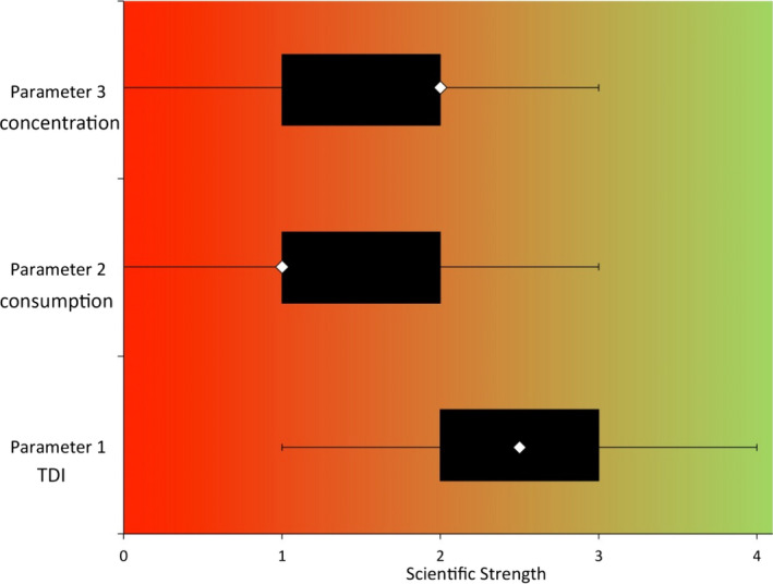
Strength of the information for parameter estimation in the melamine risk assessment. The diamond shows the median of scores of all seven experts on all four dimensions, the black box the interquartile range and the error bars the range of all scores. Colour shading ranges from green to reflect high parameter strength to red to reflect low parameter strength

Figure B.4.

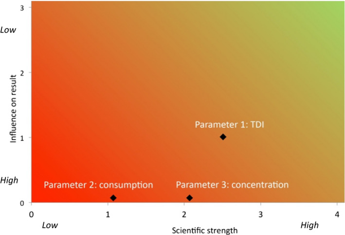
Strength and influence diagram for parameter uncertainty in the melamine risk assessment. The diamond shows the median of scores of all seven experts on all four dimensions for strength and the median score of all seven experts for influence. Colour shading ranges from green to reflect high parameter strength and low influence to red to reflect low parameter strength and high influence

Considering the group's experience, there needs to be a common understanding of interpretation of the risk management question before the NUSAP session starts. The four dimensions to evaluate parameter strength reflected different aspects of the knowledge base, but were also related and personal interpretations of the exact nature of these dimensions and their scales differed between group members. Therefore, precise definitions and training of experts to understand these definitions are prerequisites to a standardised application of the NUSAP methodology. The influence of a parameter on the risk assessment conclusion can be evaluated by only considering the impact of changes in the parameter value on the risk assessment conclusion (comparable to local sensitivity analysis, see Annex B.17). Alternatively, the plausible range over which a parameter may vary and parameter interactions can also be taken into account (comparable to global sensitivity analysis). These two interpretations may lead to different conclusions about parameter influence, and experts need to agree on the interpretation before scoring.

Strengths

1. Pedigree criteria encourage systematic and consistent consideration of different aspects of uncertainty for each element of an assessment, providing a relative measure of its scientific strength.

2. Can inform the prioritisation of uncertain elements in the risk assessment by combining the assessment of scientific strengths with an evaluation of the influence of each element on the assessment conclusion using expert judgement.

3. As for other structured judgement approaches, when used in a workshop format NUSAP provides a framework for involving additional experts in an iterative process which should improve the quality of the uncertainty analysis.

4. The NUSAP method could in principle be applied in any area of EFSA's work provided that training is given.

Weaknesses and how to address them

1. The pedigree criteria may be interpreted in different ways by different participants due to ambiguity of the verbal definitions.

2. The current pedigree matrices may not be fully applicable to EFSA's work. However, users are free to adapt it to their own purposes.

3. Applying the NUSAP method is more complex than working with ordinal scales.

4. The NUSAP method does not provide an evaluation of the combined effect of multiple uncertainties and therefore needs to be used in conjunction with other methods.

5. Combining scores for different criteria and different experts by taking median lacks theoretical basis and produces an ordinal scale for strengths without defined meaning. They can nevertheless be used as relative measure of strength of evidence.

6. Holding workshops to apply the NUSAP method has costs and time implications. In principle, this could be reduced (but not eliminated) by using pedigree matrices and diagnostic diagrams within a normal Working Group procedure.

Assessment against evaluation criteria

This method is assessed against the criteria in Table B.9.

Table B.9.

Assessment of NUSAP approach (when applied well) against evaluation criteria

Criteria	Evidence of current acceptance	Expertise needed to conduct	Time needed	Theoretical basis	Degree/extent of subjectivity	Method of propagation	Treatment of uncertainty & variability	Meaning of output	Transparency and reproducibility	Ease of understanding for non‐specialist
Stronger characteristics	International guidelines or standard scientific method	No specialist knowledge required	Hours	Well established, coherent basis for all aspects	Judgement used only to choose method of analysis	Calculation based on appropriate theory	Different types of uncertainty & variability quantified separately	Range and probability of possible answers	All aspects of process and reasoning fully documented	All aspects fully understandable
	EU level guidelines or widespread in practice	Can be used with guidelines or literature	Days	Most but not all aspects supported by theory	Combination of data and expert judgement	Formal expert judgement	Uncertainty & variability quantified separately	Range and relative possibility of answers	Most aspects of process and reasoning well documented	Outputs and most of process understandable
	National guidelines, or well established in practice or literature	Training course needed	Weeks	Some aspects supported by theory	Expert judgement on defined quantitative scales	Informal expert judgement	Uncertainty & variability distinguished qualitatively	Range of answers but no weighting	Process well documented but limited explanation of reasoning	Outputs and principles of process understandable
	Some publications and/or regulatory practice	Substantial expertise or experience needed	A few months	Limited theoretical basis	Expert judgement on defined ordinal scales	Calculation or matrices without theoretical basis		Quantitative measure of degree of uncertainty	Limited explanation of process and/or basis for conclusions	Outputs understandable but not process
Weaker characteristics	Newly developed	Professional statistician needed	Many months	Pragmatic approach without theoretical basis	Verbal description, no defined scale	No propagation	No distinction between uncertainty & variability	Ordinal scale or narrative description for degree of uncertainty	No explanation of process or basis for conclusions	Process and outputs only understandable for specialists

Conclusions

1. The NUSAP method can be used as a qualitative approach to help prioritise uncertain elements in risk assessment for quantitative analysis by other methods.

2. NUSAP may be especially useful as a structured approach for qualitative characterisation of uncertainties which are not included in quantitative assessment.

3. NUSAP practitioners encourage its use in a structured workshop format with groups of experts. As for other formal approaches, this requires additional time and resources but increases the chance of detecting relevant uncertainties and provides a more considered characterisation of their impact on the assessment.

4. The NUSAP method should be further evaluated in a series of case studies for EFSA.

5. A common terminology should be developed for use in NUSAP assessments, which is understood by all involved.

References

Boone I, Van der Stede Y, Bollaerts K, Vose D, Maes D, Dewulf J, Messens W, Daube G, Aerts M and Mintiens K, 2009 NUSAP method for evaluating the data quality in a quantitative microbial risk assessment model for Salmonella in the pork production chain. Risk Anal 2009;29:502‐517.

Bouwknegt M, Knol AB, van der Sluijs JP and Evers EG, 2014. Uncertainty of population risk estimates for pathogens based on QMRA or epidemiology: a case study of Campylobacter in the Netherlands. Risk Anal 2014;34:847‐864.

Funtowicz SO and Ravetz JR, 1993. Science for the post‐normal age. Futures 1993;25:735‐755.

Van der Sluijs JP, Craye M, Funtowicz S, Kloprogge P, Ravetz J and Risbey J, 2005. Combining quantitative and qualitative measures of uncertainty in model‐based environmental assessment: the NUSAP system. Risk Anal. 2005;25:481‐492.

Vose Consulting, 2010. A quantitative microbiological risk assessment of Campylobacter in the broiler meat chain. Boulder, CO (updated report 2011). EFSA Technical Report 132. http://www.efsa.europa.eu/it/search/doc/132e.pdf

Vose Consulting, 2011. A Quantitative Microbiological Risk Assessment of Salmonella spp. in broiler (Gallus gallus) meat production. Boulder, CO. EFSA Technical report 183. http://www.efsa.europa.eu/it/supporting/doc/183e.pdf

B.5. Uncertainty tables for quantities

Purpose, origin and principal features

An EFSA guidance document on dealing with uncertainty in exposure assessment (EFSA, 2006) suggested using a tabular approach to identify and qualitatively evaluate uncertainties. Three types of tables were proposed, serving complementary functions in the assessment. The first two tables were designed to help assessors identify uncertainties in different parts of exposure assessment. The third table provided a template for assessors to evaluate the individual and combined impacts of the identified uncertainties on their assessment, using plus and minus symbols to indicate the direction and magnitude of the impacts. This section is focussed on this last type of table.

The original purpose of the table was threefold: to provide an initial qualitative evaluation of the uncertainty to assist in deciding whether a quantitative assessment is needed; to assist in targeting quantitative assessment (when needed) on the most important sources of uncertainty; and to provide a qualitative assessment of those uncertainties that remain unquantified. In practice, it has mostly been applied for the latter purpose, at the end of the assessment.

The approach is very general in nature and can be applied to uncertainties affecting any type of quantitative estimate. Therefore, although it was originally designed for evaluating uncertainties in human dietary exposure assessment, it is equally applicable to quantitative estimates in any other area of scientific assessment. It is less suitable for uncertainties affecting categorical questions, for which different tabular approaches have been devised (see Annex B.6).

The principal features of the method are the listing of uncertainties and evaluation of their individual and combined impacts on the quantitative estimate in question, presented in a table with two or more columns. The impacts are usually expressed using plus and minus symbols, indicating the direction and, in some cases, the magnitude of the impact. In early examples of the approach, the meaning of the plus and minus symbols was described qualitatively (e.g. small, medium, large impacts), but in some later examples a quantitative scale is provided (see below). The most up‐to‐date detailed description of the approach is included in a paper by Edler et al. (2013, their Section 4.2).

Applicability in areas relevant for EFSA

EFSA (2006, 2007) introduced the tabular approach and provided an example, but no detailed guidance. The most frequent user has been the CONTAM Panel, which has used a version of the third type of table in almost all of their Opinions since 2008, and extended it to include uncertainties affecting hazard and risk as well as exposure. CONTAM's version of the table lists the uncertainties affecting their assessment, and indicates the direction of the impact of each individual uncertainty on the assessment conclusion: + for uncertainties that cause overestimation of exposure or risk, and – for those that cause underestimation. CONTAM initially attempted to indicate the magnitude of the uncertainty by using one, two or three + or – signs, but ultimately decided to use only one + or −, or a combination of both (+/−), due to the difficulty in assigning magnitude. CONTAM provide a qualitative (verbal) evaluation of the combined impact of the uncertainties in text accompanying the table.

The ANS Panel have for some years used uncertainty tables similar to those of EFSA (2006, 2007) and the CONTAM Panel and the Scientific Committee have included an uncertainty table in one of their Opinions (EFSA, 2014a). Variants of the tabular approach have been used in Opinions and Guidance Documents by PPR Panel (e.g. EFSA, 2007, 2008, 2012), a CEF Panel Opinion on bisphenol A (EFSA, 2015) and an Opinion of the PLH Panel (EFSA, 2014b). Some of these included scales defining quantitative ranges for the + and – symbols (see example below). In some cases, the meaning of the + and – symbols was reversed (+ meaning the real exposure or risk may be higher than the estimate, rather than that the estimate is an overestimate).

The EFSA (2006, 2007) approach has been taken up in modified form by other EU risk assessment authorities. The ECHA (2008) guidance on uncertainty analysis includes two types of uncertainty table, adapted from those in EFSA (2006, 2007). One type of table is used for identifying uncertainties in exposure and effect assessment, while the other is used for evaluating the individual and combined impact of the identified uncertainties on exposure, hazard and risk. The latter table uses + symbols to indicate over‐estimation and – for underestimation. One, two or three symbols indicate low, moderate and high magnitude, respectively. Similarly, a SCENIHR (2012) memorandum on weight of evidence includes a table for evaluating uncertainty that is closely related to the EFSA (2006, 2007) tables. Aspects of uncertainty are listed together with evaluations of their nature, their magnitude and direction, and their importance for the risk assessment.

Edler et al. (2013) describe the application of uncertainty tables for evaluating unquantified those uncertainties that are not quantified by the BMDL in benchmark dose modelling for genotoxic carcinogens. They use uncertainty tables similar to those of EFSA (2006, 2007), with + and – symbols defined on a quantitative scale and expressing how much higher or lower the BMDL would be, if adjusted to take account of the unquantified uncertainties that have not been quantified. Edler et al. (2013) provide step‐by‐step guidance on both forms of uncertainty table. Their instructions emphasise the importance of guarding against cognitive biases that tend to affect expert judgement, drawing on ideas from expert elicitation methodology. Annexes to the paper include case studies for the dye Sudan 1 and for PhIP, which is produced during the grilling and frying of meat and fish.

Potential contribution to major elements of uncertainty analysis

Potential contribution of the uncertainty tables approach described in this section to major elements of uncertainty analysis.

Elements in uncertainty analysis	Potential contribution of this approach
Identifying uncertainties	Not applicable (provides a framework within which identified uncertainties may be summarised)
Characterising uncertainties	Ordinal scale for the impact of each uncertainty on the assessment output, in some cases with quantitative definitions for the scale
Combining uncertainties	May be assessed by expert judgement and expressed using the same scale as for characterising uncertainties
Prioritising uncertainties	The relative contribution of individual uncertainties can be assessed by comparing their evaluations in the uncertainty table

Melamine example

Members of the Working Group used a modified form of uncertainty table to assess uncertainties affecting three parameters in the example assessment of melamine, based on the context described in Annex B.2. The group evaluated the individual and combined impacts of these parameters on the uncertainty of the following question: does the possible worst‐case exposure of high‐consuming European children to melamine from consumption of chocolate containing contaminated Chinese milk powder exceed the relevant health‐based guidance value, and if so by how much?

The group evaluated the uncertainties on a scale that was previously used in an opinion on BPA (EFSA, 2015). This scale uses plus and minus symbols with quantitative definitions in terms of how much lower or higher a real value might plausibly be compared to its estimate, as shown in Figure B.5. Note that the size of the intervals can be adjusted for different assessments, depending on the scale of uncertainties that are present (Edler et al., 2013).

Figure B.5.

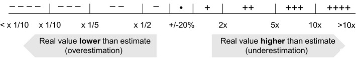
Scale used for assessing uncertainty in example evaluation (Table B.10)

The group members were asked to assess the uncertainty of each individual parameter, and also to assess the combined impact of all three parameters on the uncertainty of the assessment output (ratio of exposure to TDI). The evaluation was conducted in two rounds, with the results from the first round being collated on‐screen and discussed before the second round. This allowed assessors to adjust their evaluations in the light of the discussion, if they wished. The results of the second round are shown in Table B.10. The third column in Table B.10 shows the range of evaluations given by the assessors for the extent to which the real value of each individual parameter could be lower than its estimate, while the fourth column shows the range of evaluations for how much the real value of the assessment output (ratio of exposure to TDI) could exceed its estimate based on the uncertainty of that parameter alone. In the bottom row, the fourth column shows the range of evaluations for how much the real value of the assessment output (ratio of exposure to TDI) could exceed its estimate based on the uncertainty of all three parameters considered together. Various methods could be considered for aggregating the judgements of the individual experts. In this example, the overall range spans the set of ranges provided by the individual assessors, and thus expresses the range of values that were considered plausible by one or more of the assessors.

Table B.10.

Example of uncertainty table for the melamine case study

Parameter	Value in EFSA (2008) assessment	Range for uncertainty of individual parameters	Range for uncertainty of assessment output
TDI	0.5mg/kg bw per day	NQ/NQ or −−−/++	NQ/NQ or −−/+++
Highest concentration of melamine in milk powder	2,563 mg/kg	−−−/+	−−−/+
Highest consumption of Chinese chocolate by children	0.044 kg	−−−/++	−−−/++
Assessment output: ratio of the calculated exposure to the TDI	269%		−−−−/NQ or −−−−/++

NQ = not quantified. See Figure B.5 for definition of scale for plus and minus symbols. See text for further explanation. Note that the results shown here differ from those in Annexes B.8 and B.9, as the latter were constructed as hypothetical examples and not elicited from experts.

One assessor was unable to quantify the uncertainty of the TDI in either direction, and one was able to quantify the upwards uncertainty but not the downwards uncertainty. These assessments are shown in the Table B.10 as NQ (not quantified). The results affected by this show first the range including all assessors, and then the range excluding the ‘NQ’ assessments.

The overall range for the output of the assessment (bottom right corner of Table B.10) can be converted to numeric form, using the scale in Figure B.5 (note this conversion uses the full width of each interval on the scale and may overstate the assessors’ actual uncertainty). One expert considered that it was not possible to quantify how much higher the real ratio of exposure to TDI could be compared to the EFSA (2008) estimate of 269%, because they were not able to quantify how different the appropriate TDI could be than that used by EFSA (2008) based on the information available in the EFSA statement. The range of uncertainty for the remaining experts was from more than 10x below the estimated ratio to 5x above it, i.e. the real worst‐case exposure for EU children eating contaminated chocolate could be below 30% of the TDI at the lower bound (or even 0 if there was no contamination), and about 13x the TDI at the upper bound (rounding to avoid over‐precision).

In this example, the approach was modified to be feasible within the time reserved for it (1–2 hours). This illustrates how it can be adapted for situations when time is short. If more time were available, it would be good practice to document briefly (in the table or in accompanying text) the uncertainties that were considered for each parameter and the reasoning for the evaluation of their impact. If a parameter was affected by several different uncertainties, it might be useful to evaluate them separately and show them in separate rows of the table. In addition, it might be desirable for the assessors to discuss the reasons for differences between their individual ranges, and if appropriate seek a consensus on a joint range (which might be narrower than the range enveloping the individual judgements).

One assessor preferred to express their judgement of the uncertainty for each parameter as a quantitative range and then derive a range for the overall uncertainty by calculation: a form of interval analysis (see Annex B.7). Interval analysis can also be applied when using the +/− scale, by converting the scores to numeric form for calculation, as was done by EFSA (2015a,b,c) when combining evaluations of uncertainty for different sources of internal BPA exposure. These examples suggest that a tabular format similar to uncertainty tables could be used to facilitate and document judgements on ranges for interval analysis.

Strengths

1. The uncertainty table makes transparent many subjective judgements that are unavoidably present in risk assessment, thus improving the quality of group discussion and the reliability of the resulting estimates, and making the judgements open to challenge by others.

2. Concise and structured summary of uncertainties facilitates evaluation of their combined impact by the assessor, even though not based on theory.

3. The approach can be applied to any area of scientific assessment.

4. The approach can be applied to all types of uncertainty, including ambiguity and qualitative issues such as study quality. Anything that the assessors identify as a factor or consideration that might alter their answer to the assessment question can be entered in the table.

5. The approach facilitates the identification of unquantifiable uncertainties, which can be recorded in the table (a question mark or NQ for not quantifiable in the right hand column).

6. The tabular format is highly flexible. It can be expanded when useful to document the evaluation more fully, or abbreviated when time is short.

7. Using a quantitative scale reduces the ambiguity of purely score‐based or narrative approaches. The symbols for the combined assessment can be converted into an approximate, quantitative uncertainty interval for use in interval analysis and to facilitate interpretation by risk managers.

8. The combined assessment helps to inform decision‐making, specifically whether the combined effect of uncertainties is clearly too small to change the decision, or whether more refined risk or uncertainty analysis is needed. But it may also suggest a false precision.

9. The main contributors to overall uncertainty are identified in a structured way, enabling their prioritisation for more quantitative assessment when required (e.g. sensitivity analysis or probabilistic modelling).

10. Tabular format provides a concise summary of the evidence and reasoning behind the assessment of overall uncertainty, increasing transparency for the reader when compared to scoring systems and narrative discussion of uncertainties.

Weaknesses and possible solutions to them

1. For some people, the approach does not seem to be immediately intuitive. Therefore, training should be provided.

2. Some users find it difficult to assess the magnitude of uncertainties. This can be mitigated by providing training similar to that which is normally provided to experts taking part in formal elicitation procedures (EFSA, 2014a,bc).

3. People are bad at making judgements about how uncertainties combine. For this reason, it is better for users to assess plausible intervals for the individual uncertainties and derive their impacts on the assessment output by interval analysis (Annex B.7).

4. The scales used to define the + and − symbols can be prone to misunderstanding. Therefore, they should be designed and communicated carefully. An alternative is for the assessors to express the magnitudes of the uncertainties as numerical intervals. This is also beneficial when assessors are able to judge the uncertainty more finely than provided for in the scale.

5. Transparency will be impaired if insufficient information is given about the reasoning for the judgements in the table, or if readers cannot easily locate supporting information provided outside the table. This can be addressed by providing more information within the table, if necessary by adding extra columns, and by including cross‐references in the table to additional detail in accompanying text and ensuring that this is clearly signposted.

6. The approach relies on expert judgement, which is subject to various psychological biases (see Section 5.9). Techniques from formal expert elicitation methodology can be used to improve the robustness of the judgements that are made; optionally, fully formal expert elicitation can be used to evaluate the overall uncertainty and/or the contribution of the most important individual uncertainties (methods described in Annexes B.8 and B.9, with hypothetical examples).

Assessment against evaluation criteria

This method is assessed against the evaluation criteria in Table B.11.

Conclusions

1. This method is applicable to all types of uncertainty affecting quantities of interest, in all areas of scientific assessment. It is flexible and can be adapted to fit within the time available, including urgent situations.

2. The method is a framework for documenting expert judgements and making them transparent. It is generally used for semi‐formal expert judgements, but formal techniques (see Annex B.9) could be incorporated where appropriate, e.g. when the uncertainties considered are critical to decision‐making.

3. The method uses expert judgement to combine multiple uncertainties. The results of this will be less reliable than calculation, it would be better to use uncertainty tables as a technique for facilitating and documenting expert judgement of quantitative ranges for combination by interval analysis. However, uncertainty tables using +/− symbols are a useful option for two important purposes: the need for an initial prioritisation of uncertainties, and to inform probability judgements in the characterisation of overall uncertainty (see Section 14 of main document).

References

ECHA, 2008. Guidance on information requirements and chemical safety assessment. Chapter R.19: Uncertainty analysis. European Chemicals Agency (ECHA).

Edler L, Hart A, Greaves P, Carthew P, Coulet M, Boobis A, Williams GM, Smith B. 2013. Selection of appropriate tumour data sets for Benchmark Dose Modelling (BMD) and derivation of a Margin of Exposure (MoE) for substances that are genotoxic and carcinogenic: Considerations of biological relevance of tumour type, data quality and uncertainty analysis. Food Chem. Toxicol., https://doi.org/10.1016/j.fct.2013.10.030

EFSA Scientific Committee, 2006. Guidance on a request from EFSA related to Uncertainties in Dietary Exposure Assessment. The EFSA Journal, 438, 1‐54.

EFSA PPR Panel (EFSA Panel on Plant protection products and their Residues), 2007. Opinion on a request from the Commission on acute dietary intake assessment of pesticide residues in fruit and vegetables. The EFSA Journal, 538, 1‐88.

EFSA PPR Panel (EFSA Panel on Plant protection products and their Residues), 2008. Scientific Opinion on the Science behind the Guidance Document on Risk Assessment for birds and mammals. The EFSA Journal (2008) 734: 1‐181.

EFSA PPR Panel (EFSA Panel on Plant protection products and their Residues), 2012. Guidance on the use of probabilistic methodology for modelling dietary exposure to pesticide residues. The EFSA Journal, 10: 1‐95.

EFSA Scientific Committee, 2014a. Scientific Opinion on the safety assessment of carvone, considering all sources of exposure. EFSA Journal 2014;12(7):3806.

EFSA PLH Panel (EFSA Panel on Plant Health), 2014b. Scientific Opinion on the risk of Phyllosticta citricarpa (Guignardia citricarpa) for the EU territory with identification and evaluation of risk reduction options. EFSA Journal 2014;12(2):3557.

EFSA (European Food Safety Authority), 2014c. Guidance on Expert Knowledge Elicitation in Food and Feed Safety Risk Assessment. EFSA Journal 2014;12(6):3734.

EFSA CEF Panel (EFSA Panel on Food Contact Materials, Enzymes, Flavourings and Processing Aids), 2015. Scientific Opinion on the risks to public health related to the presence of bisphenol A (BPA) in foodstuffs – Part: exposure assessment. EFSA Journal 2015;13(1):3978.

Hart A, Gosling JP, Boobis A, Coggon D, Craig P and Jones D. 2010. Development of a framework for evaluation and expression of uncertainties in hazard and risk assessment. Research Report to Food Standards Agency, Project No. T01056.

SCENIHR Committee, 2012. Memorandum on the use of the scientific literature for human health risk assessment purposes – weighing of evidence and expression of uncertainty. DG SANCO, European Commission, Brussels.

Table B.11.

Assessment of Uncertainty tables for quantities (when applied well) against evaluation criteria

Criteria	Evidence of current acceptance	Expertise needed to conduct	Time needed	Theoretical basis	Degree/extent of subjectivity	Method of propagation	Treatment of uncertainty & variability	Meaning of output	Transparency and reproducibility	Ease of understanding for non‐specialist
Stronger characteristics	International guidelines or standard scientific method	No specialist knowledge required	Hours	Well established, coherent basis for all aspects	Judgement used only to choose method of analysis	Calculation based on appropriate theory	Different types of uncertainty & variability quantified separately	Range and probability of possible answers	All aspects of process and reasoning fully documented	All aspects fully understandable
	EU level guidelines or widespread in practice	Can be used with guidelines or literature	Days	Most but not all aspects supported by theory	Combination of data and expert judgement	Formal expert judgement	Uncertainty & variability quantified separately	Range and relative possibility of answers	Most aspects of process and reasoning well documented	Outputs and most of process understandable
	National guidelines, or well established in practice or literature	Training course needed	Weeks	Some aspects supported by theory	Expert judgement on defined quantitative scales	Informal expert judgement	Uncertainty & variability distinguished qualitatively	Range of answers but no weighting	Process well documented but limited explanation of reasoning	Outputs and principles of process understandable
	Some publications and/or regulatory practice	Substantial expertise or experience needed	A few months	Limited theoretical basis	Expert judgement on defined ordinal scales	Calculation or matrices without theoretical basis		Quantitative measure of degree of uncertainty	Limited explanation of process and/or basis for conclusions	Outputs understandable but not process
Weaker characteristics	Newly developed	Professional statistician needed	Many months	Pragmatic approach without theoretical basis	Verbal description, no defined scale	No propagation	No distinction between uncertainty & variability	Ordinal scale or narrative description for degree of uncertainty	No explanation of process or basis for conclusions	Process and outputs only understandable for specialists

B.6. Uncertainty tables for questions

Purpose, origin and principal features

The purpose of this method is to provide a structured approach for addressing uncertainty in weight of evidence assessment of a question of interest and expressing the uncertainty of the conclusion. Weight of evidence as an overall process will be considered in more detail in a separate mandate.7

The method described here was developed by Hart et al. (2010), who noted that uncertainty tables of the type described by EFSA (2006, 2007) address uncertainty in quantitative estimates (e.g. exposure, reference dose) and are not well suited to addressing uncertainty in categorical questions, which involve choices between two or more categories.

The principal features of this method are the use of a tabular approach to summarise the assessment of multiple lines of evidence and their associated uncertainties, and the expression of conclusions in terms of the probability of alternative categories. The tabular approach provides a structured framework, which is intended to help the assessors develop the assessment and improve its transparency. The expression of conclusions as probabilities is intended to avoid the ambiguity of narrative forms, and also opens up the possibility of using probability theory to help form overall conclusions when an assessment comprises a series of linked categorical and/or quantitative questions.

The main steps of the approach can be summarised as follows:

1. Define clearly the question(s) to be answered.

2. Identify and describe relevant lines of evidence (LoE).

3. Organise the LoE into a logical sequence to address the question of interest.

4. Identify their strengths, weaknesses and uncertainties.

5. Evaluate the weight of each LoE and its contribution to answering the question.

6. Take account of any prior knowledge about the question.

7. Make an overall judgement about the balance of evidence, guarding against cognitive biases associated with expert judgement, and use formal elicitation methods if appropriate.

8. Express the conclusion as a probability or range of probabilities, if possible, and explain the reasoning that led to it.

Applicability in areas relevant for EFSA

The approach is, in principle, applicable to any two‐category question in any area of EFSA's work. It would be possible to adapt it for questions with multiple categories (e.g. choices between 3 or more modes of action), although this would be more complex. It provides a more structured approach to weight of evidence than the traditional approach of a reasoned argument in narrative text, and a less ambiguous way of expressing the conclusion. However, it is intended to complement those approaches rather than completely replace them, because it will always be desirable to accompany the tabular summary of the assessment with a detailed narrative description of the evidence and reasoning, and it may aid communication to accompany numerical probabilities with narrative statements of the conclusion.

The approach has so far been used in only a few assessments. The original research report contains a simplified example of hazard identification for caffeine (Hart et al., 2010). Edler et al. (2014) provide step‐by‐step instructions for applying the method to assess the probability that chemicals are genotoxic carcinogens, and detailed case studies for Sudan 1 and PhIP. It was used for hazard identification in the EFSA (2015a,b,c) Opinion on bisphenol A (BPA), assessing the probability that BPA has the capability to cause specific types of effects in animals based on evidence from a wide variety of studies. In the same Opinion, probability was also used to express judgements about the relevance to humans of effects seen animals and whether, if they occurred in humans, they would be adverse. Evidence for the judgements about relevance and adversity were discussed in the text of the opinion, rather than by tabulated lines of evidence.

Potential contribution to major elements of uncertainty analysis

Elements in uncertainty analysis	Potential contribution of this approach
Identifying uncertainties	Structured approach promotes identification of uncertainties affecting individual lines of evidence and overall conclusion
Characterising uncertainties	Concise narrative description of each line of evidence including strengths, weaknesses and uncertainties. Strengths, weaknesses and uncertainties of individual lines of evidence and their impact on the conclusion are assessed by expert judgement
Combining uncertainties	The combined impact of all the lines of evidence and their uncertainties is assessed by expert judgement and expressed as a probability or range of probabilities for a positive conclusion
Prioritising uncertainties	The relative importance of uncertainties affecting individual lines of evidence can be assessed by considering the weaknesses identified in the table. The ordinal scale for influence indicates what each line of evidence contributes to the balance of probability (uncertainty) for the conclusion

Melamine example

The EFSA (2008) Statement states that ‘the primary target organ for melamine toxicity is the kidney’. Here, the use of uncertainty tables for categorical questions is illustrated by applying the approach to summarise the evidence that melamine causes kidney effects. Although the evidence in this case is rather one‐sided, it serves to illustrate the principles of the approach.

The first step is to specify in precise terms the question to be considered. In this case, the question was defined as follows: does melamine have the capability to cause adverse effects on kidney in humans? Note that the biological process underlying this is a dose–response relationship, so the question could alternatively be framed as a quantitative question.

The assessment was carried out by three toxicologists in the Working Group. First, they were asked to identify the main lines of evidence for assessing the potential for melamine to cause kidney effects, which were available at the time of the EFSA (2008) statement. Four lines of evidence were identified, as listed and briefly described in Table B.12. The assessors were then asked to consider the influence of each line of evidence on their judgement about the answer to the question, and to express this using a scale of arrow symbols which are defined in Table B.13. Upward arrows indicate an upward influence on the likelihood that melamine causes kidney effects, and the number of arrows indicates the strength of the influence. Next, the assessors were asked to make a judgement about the probability that melamine causes kidney effects, considering all lines of evidence together. They were asked to express this probability using another scale, defined in Table B.14. The assessors made their judgements for both influence and probability individually. The judgements were then collected and displayed on screen for discussion, and the assessors were given the opportunity to adjust their judgements if they wished. Table B.12 shows the range of judgements between assessors. In this case, there was little variation between assessors in their assessment of influence, and all three gave the same conclusion: that it is very likely (probability 90–100%) that melamine has the potential to cause adverse effects kidney in humans.

Table B.12.

Assessment of evidence and uncertainty for the question: does melamine have the capability to cause adverse effects on kidney in humans?

Lines of evidence	Influence on conclusion
Line of Evidence 1 – animal studiesSame effect on more than one species	↑↑↑
Line of Evidence 2 – information on effects in humansSevere health effect in humans but unspecified in the EFSA statement	↑/↑↑
Line of Evidence 3 – information on mode of actionInformation on crystal formation in kidneys. Effect not dependent on metabolism indicating similar effects are likely in different species	↑/↑↑
Line of Evidence 4 – Evidence of adverse effects in companion animalsKidney toxicity in cats with crystal formation resulting from melamine adulterated pet food	↑/↑↑
CONCLUSION (by semi‐formal expert judgement, see text) Based on the consistency from the different lines of evidence	Very likely(90–100% probability)

See Table B.13 for key to symbols and Table B.14 for probability scale. Pairs of symbols separated by a slash (↑/↑↑) represent variation of judgements between assessors.

Table B.13.

Key to scale of symbols used to express the influence of lines of evidence on the answer to the question in Table B.12

Symbol	Influence on probability of positive answer to question
↑↑↑	Strong upward influence on probability
↑↑	Intermediate upward influence on probability
↑	Minor upward influence on probability
●	No influence on probability
↓	Minor downward influence on probability
↓↓	Intermediate downward influence on probability
↓↓↓	Strong downward influence on probability
?	Unable to evaluate influence on probability

Table B.14.

Scale used for expressing the probability of a positive answer to the question addressed in Table B.12, after Mastrandrea et al. (2010)

Term	Probability of outcome
Virtually certain	99–100% probability
Very likely	90–100% probability
Likely	66–100% probability
As likely as not	33–66% probability
Unlikely	0–33% probability
Very unlikely	0–10% probability
Exceptionally unlikely	0–1% probability

Due to the limited time that was set for developing this example, Table B.12 provides only very limited explanation for the judgements made in assessing individual lines of evidence and the final conclusion. More explanation should be provided in a real assessment, including an indication of the relevance and reliability of each line of evidence, and the reasoning for the final conclusion. This may be done either within the table (adding extra content and/or columns, e.g. Annex C of EFSA, 2015a,b,c), or in accompanying text. However, more abbreviated formats may sometimes be justified (e.g. in urgent situations).

The procedure adopted for making judgements in this example may be regarded as semi‐formal, in that a structured approach was used in which experts considered their judgements individually and then reviewed them after group discussion. Ideally, it would be preferable to use a fully formal expert elicitation procedure (see Annex B.9), especially for weight of evidence questions that have a large impact on the assessment conclusion.

Strengths

1. Promotes a structured approach to weighing multiple lines of evidence and taking account of their uncertainties, which should help assessors in making their judgements and potentially lead to better conclusions.

2. Expressing the (uncertainty of the) conclusion in terms of probability avoids the ambiguity of narrative conclusions, although care is needed to avoid suggesting false precision.

3. Compatible with formal approaches to eliciting expert judgements on the probability of the conclusion.

4. The judgements involved can be made by formal EKE, which would ideally be preferable. When judgements are made less formally, the process can still be designed to encourage assessors to guard against common cognitive biases.

5. Tabular structure is intended to make the evidence and reasoning more accessible, understandable and transparent for scientific peers, risk managers and stakeholders.

Weaknesses and possible approaches to address them

1. Tabular structure can become cumbersome if there are many lines of evidence and/or extensive detail is included. This can be addressed by careful management of the quantity, organisation (e.g. grouping similar studies) and format of table content, and by providing necessary additional detail in accompanying text.

2. For some types of question, probabilities may be misinterpreted as frequencies or risks (e.g. probability of chemical X having a carcinogenic mode of action may be misinterpreted as the probability of an individual getting cancer). This should be avoided by good communication practice.

3. Some assessors may be unwilling to give numerical probabilities. Can be addressed by using a scale of likelihood terms (e.g. EFSA, 2014a,b), preferably with quantitative definitions.

4. This approach is best suited to questions with two categories, and becomes cumbersome for questions with more categories.

Assessment against evaluation criteria

This method is assessed against the criteria in Table B.15.

Table B.15.

Assessment of Uncertainty tables for questions of interest (when applied well) against evaluation criteria

Criteria	Evidence of current acceptance	Expertise needed to conduct	Time needed	Theoretical basis	Degree/extent of subjectivity	Method of propagation	Treatment of uncertainty & variability	Meaning of output	Transparency and reproducibility	Ease of understanding for non‐specialist
Stronger characteristics	International guidelines or standard scientific method	No specialist knowledge required	Hours	Well established, coherent basis for all aspects	Judgement used only to choose method of analysis	Calculation based on appropriate theory	Different types of uncertainty & variability quantified separately	Range and probability of possible answers	All aspects of process and reasoning fully documented	All aspects fully understandable
	EU level guidelines or widespread in practice	Can be used with guidelines or literature	Days	Most but not all aspects supported by theory	Combination of data and expert judgement	Formal expert judgement	Uncertainty & variability quantified separately	Range and relative possibility of answers	Most aspects of process and reasoning well documented	Outputs and most of process understandable
	National guidelines, or well established in practice or literature	Training course needed	Weeks	Some aspects supported by theory	Expert judgement on defined quantitative scales	Informal expert judgement	UNCERTAINTY & VARIABILITY DISTINGUISHED QUALITATIVELY	Range of answers but no weighting	Process well documented but limited explanation of reasoning	Outputs and principles of process understandable
	Some publications and/or regulatory practice	Substantial expertise or experience needed	A few months	Limited theoretical basis	Expert judgement on defined ordinal scales	Calculation or matrices without theoretical basis		Quantitative measure of degree of uncertainty	Limited explanation of process and/or basis for conclusions	Outputs understandable but not process
Weaker characteristics	Newly developed	Professional statistician needed	Many months	Pragmatic approach without theoretical basis	Verbal description, no defined scale	No propagation	No distinction between uncertainty & variability	Ordinal scale or narrative description for degree of uncertainty	No explanation of process or basis for conclusions	Process and outputs only understandable for specialists

Conclusions

1. This approach is potentially applicable to any type of binary question in all areas of EFSA's work, and to all types of uncertainty affecting those questions.

2. The approach is new and would benefit from further case studies to evaluate its usefulness and identify improvements.

References

Edler L, Hart A, Greaves P, Carthew P, Coulet M, Boobis A, Williams GM, and Smith B. 2014. Selection of appropriate tumour data sets for Benchmark Dose Modelling (BMD) and derivation of a Margin of Exposure (MoE) for substances that are genotoxic and carcinogenic: Considerations of biological relevance of tumour type, data quality and uncertainty analysis. Food Chem. Toxicol., 70: 264–289. https://doi.org/10.1016/j.fct.2013.10.030

EFSA Scientific Committee, 2006. Guidance of the Scientific Committee on a request from EFSA related to Uncertainties in Dietary Exposure Assessment. The EFSA Journal, 438, 1–54.

EFSA, (European Food Safety Authority), 2008. Statement of EFSA on risks for public health due to the presences of melamine in infant milk and other milk products in China. EFSA Journal (2008) 807, 1–10. http://www.efsa.europa.eu/sites/default/files/scientific_output/files/main_documents/807.pdf

EFSA CEF Panel (EFSA Panel on Food Contact Materials, Enzymes, Flavourings and Processing Aids), 2015. Scientific Opinion on the risks to public health related to the presence of bisphenol A (BPA) in foodstuffs: PART II – Toxicological assessment and risk characterisation. EFSA Journal 2015;13(1):3978, 621 pp. https://doi.org/10.2903/j.efsa.2015.3978

Hart A, Gosling JP, Boobis A, Coggon D, Craig P and Jones D, 2010. Development of a framework for evaluation and expression of uncertainties in hazard and risk assessment. Research Report to Food Standards Agency, Project No. T01056.

Mastrandrea MD, Field CB, Stocker TF, Edenhofer O, Ebi KL, Frame DJ, Held H, Kriegler E, Mach KJ, Matschoss PR, Plattner G‐K, Yohe GW, and Zwiers FW, 2010: Guidance Note for Lead Authors of the IPCC Fifth Assessment Report on Consistent Treatment of Uncertainties. Intergovernmental Panel on Climate Change (IPCC). Available at: http://www.ipcc.ch

B.7. Interval analysis

Origin, purpose and principal features

Interval analysis is a method to obtain a range of values for the output of a calculation or quantitative model based on specified ranges for the inputs to the calculation. If each input ranges expresses uncertainty about the corresponding input value, the output range is an expression of uncertainty about the output.

Interval analysis (also ‘interval arithmetic’, ‘interval mathematics’, ‘interval computation’) was developed by mathematicians since the early 1950s (Dwyer, 1951, as one of the first authors) to propagate errors or account for parameter variability. Modern interval analysis was introduced by Ramon E. Moore in 1966. Ferson & Ginzburg, 1996 proposed interval analysis for the propagation of ignorance (epistemic uncertainty) in conjunction with probabilistic evaluation of variability. The interval method is also discussed in the WHO‐harmonisation document, 2008, along the concept of Ferson (1996).

Interval analysis is characterised by the application of upper and lower bounds to each parameter, instead of using a fixed mean or worst‐case parameter (e.g. instead of the fixed value 1.8 for mean body height of northern males one can use the interval 1.6–2.0 to account for the variability in the population). To yield a lower bound of an estimate, all parameter values between the bounds are combined in the model that result in the lowest estimate possible. To yield the upper bound of an estimate analogously, the parameter values between the bounds are combined that yield the highest estimate possible. The interval between the lower and the upper bound estimate is then considered to characterise the uncertainty and variability around the estimate.

For uncertainty analysis, where the range for each input covers all values considered possible, the range for the output then also covers all possible values. If it is desired to specify an input range covering a subset of possible values and accompanied by a probability, the method of probability bounds analysis (Annex B.13) is more likely to be useful.

Applicability in areas relevant for EFSA

Within EFSA, the method is often used for the treatment of left‐censored data (e.g. in the exposure analysis for chemical risk assessment, EFSA, 2010a,b). If samples are included in a statistical analysis that have concentrations below the limit of detection (LOD), a lower bound estimate can be constructed by assuming that all sample concentrations < LOD are 0, and a higher bound by assuming that all sample concentrations are equal to the LOD. The true value will lie in between those values (e.g. EFSA, 2015).

Potential contribution to major elements of uncertainty analysis

Elements in uncertainty analysis	Potential contribution of this approach
Identifying uncertainties	Not applicable
Characterising uncertainties	Yes, the uncertainty is expressed for each individual uncertainty as a lower and as an upper bound
Combining uncertainties	Yes, range of output values, taking into account the range of all input parameters at the same time and making no assumptions about dependencies
Prioritising uncertainties	Not applicable

Melamine example

As described in more detail in Annex C, exposure e is calculated according to

$$e=\frac{c\times w\times q}{\mathit{bw}}$$

where

c: concentration of melamine in adulterated milk powder (mg/kg)

w: weight fraction of milk powder in chocolate

q: consumption of chocolate in a day (kg/day)

bw: body weight of consumer (kg)

The variables q and bw are both expected to be positively correlated with the age of the child and as a result to be correlated with each other. As a simple example of an approach to address dependencies in an interval analysis, the method was applied to two subpopulations of children that might be expected to have higher exposure: children aged 1 and children aged 6. These groups two were selected for illustration because of the low body weight of the younger group and a judgement that the older age group might consume as much as older children but have lower body weight. A full assessment would in principle apply the method separately to each age from 1 to 10.

For the concentration c, the highest observed level in the data used in the melamine statement was 2,563 mg/kg. This value however will not be the highest of the whole ensemble of possible values, because only a subsample has been analysed and not all samples in the ensemble. Knowing that melamine is used to mimic the N‐content of milk that should be contained in the samples, but is not, it can be assumed that the higher bound for the melamine content is the amount needed to mimic 100% milk that should be contained in the sample. Multiplying the ratio between the N‐content of milk protein and melamine (0.13/0.67 = 0.22) and the protein content in dry milk (3.4 g protein in cow milk/130 g dry matter = 26 g/kg) the maximal content of melamine in dry milk yields a higher bound of 6,100 mg/kg melamine in adulterated milk powder. The lower bound for melamine will be 0 mg/kg, because it is not naturally occurring, but the result of adulteration.

For the weight fraction of milk powder in milk chocolate w, the legally required minimum of 0.14 is chosen as the lower bound, and the highest value found in an internet search (0.28) as the higher bound.

For q, no data were available for high chocolate consumption. The assessors made informal judgements of 50 g and 300 g, for a 1‐year‐old and a 10‐year‐old child, respectively. In a real situation, expert knowledge elicitation (Annexes B.8 and B.9) would be used to obtain these numbers.

For the lower and higher bound for body weight (bw) in both age groups, the assessors used low and high percentiles from WHO growth charts as a starting point for choosing more the more extreme values in the tables below to be absolute lower and upper bounds. Again, in a real situation, expert knowledge elicitation would be used to obtain these numbers.

Child 1 year old

Parameter/Estimate	Value	Lower bound	Higher bound
c (mg/kg)	29	0	5,289 (highest observed level: 2,563)
w (‐)	0.25	0.14	0.28
q (kg/d)	0.042	0	0.05
bw (kg)	20	6	13
e (mg/d kg‐bw)	0.015225	0	14.2

Child 6 years

Parameter/Estimate	Value	Lower bound	Higher bound
c (mg/kg)	29	0	6,100 (highest observed level: 2,563)
w (‐)	0.25	0.14	0.28
q (kg/d)	0.042	0	0.3
bw (kg)	20	12	34
e (mg/d kg‐bw)	0.015225	0	42.7

In the tables above, the intervals cover both uncertainty and variability in the parameters. Below, we aim to demonstrate how also within the interval method uncertainty and variability might be treated separately (example for the 1‐year‐old child).

Child 1 year old, mainly variability

Parameter/Estimate	Valuea	Lower bound	Higher boundb
c (mg/kg)	29	0	2,563
w (‐)	0.25	0.14	0.28
q (kg/d)	0.042	0	0.05
bw (kg)	20	6	13
e (mg/d kg‐bw)	0.015	0	6.0

^aThese values are not part of the interval analysis, only demonstrate the values around which the variability/uncertainty analysis is constructed.

^bThe higher bound exposure is calculated by using the higher bound for the first three parameters and the lower bound for the body weight, denoted in bold.

Child 1 year old, uncertainty about the worst‐case (wc) values for parameters

Parameter/Estimate	Favoured valuea for wc	Lower bound for wc value	Higher bound for wc value
c (mg/kg)	2,563	2,563	6,100
w (‐)	0.28	0.28	0.30
q (kg/d)	0.05	0.05	0.1
bw (kg)	6	5.5	6.5
e (mg/d kg‐bw)	6.0	5.5	33.3

^aThese values are not part of the interval analysis, only demonstrate the values around which the variability/uncertainty analysis is constructed.

Strengths

1. The method is relatively easy to perform and straightforward. It is particularly useful as a screening method to quickly assess whether more sophisticated quantitative uncertainty analysis is needed or whether, even for an upper bound, for example, of an exposure, no concern exists. Ferson and Ginzburg, 1996 recommend it as an alternative method to probabilistic uncertainty analysis when the shape of the distribution is not known (e.g. for assessing uncertainty due to ignorance, see above).

2. When used with real upper and lower limits the method covers all possible scenarios.

Weaknesses and possible approaches to reduce them

1. Only quantifies range not probabilities within range. Therefore, useful as initial screen to determine whether probabilistic assessment is needed.

2. Most of the time it is not made clear what the ranges really are meant to represent (minimum/maximum, certain percentiles, etc.). This can be cured by transparent communication in the text and by attempting to be as consistent as possible.

3. The method does not incorporate dependencies between variables, so that the interval of the final estimate will be larger than the range of the true variability and uncertainty, if dependencies between variables occur. This limitation can be partly addressed by using scenarios representing different combinations of input variables to explore the potential impact of dependencies, as illustrated in the example above.

4. The more parameters are involved the larger will become the uncertainty range, and the more likely it is that a probabilistic assessment taking account of dependencies will be required for decision‐making. Nevertheless, since interval analysis is much simpler to perform, it is still useful as a screening method to determine whether more sophisticated analysis is needed.

5. Variability and uncertainty are not separated by the concept behind this method and it is easy to forget that both uncertainty and variability are included in the range when it is applied to uncertain variability. However, because the interval method is a special case of probability bounds analysis, the method described in Annex B.13 for addressing problems with uncertain variability could be used in conjunction with interval analysis.

Assessment against evaluation criteria

This method is assessed against the criteria in Table B.16.

Table B.16.

Assessment of Interval analysis (when applied well) against evaluation criteria

Criteria	Evidence of current acceptance	Expertise needed to conduct	Time needed	Theoretical basis	Degree/extent of subjectivity	Method of propagation	Treatment of uncertainty and variability	Meaning of output	Transparency and reproducibility	Ease of understanding for non‐specialist
Stronger characteristics	International guidelines or standard scientific method	No specialist knowledge required	Hours	Well established, coherent basis for all aspects	Judgement used only to choose method of analysis	Calculation based on appropriate theory	Different types of uncertainty & variability quantified separately	Range and probability of possible answers	All aspects of process and reasoning fully documented	All aspects fully understandable
	EU level guidelines or widespread in practice	Can be used with guidelines or literature	Days	Most but not all aspects supported by theory	Combination of data and expert judgement	Formal expert judgement	Uncertainty & variability quantified separately	Range and relative possibility of answers	Most aspects of process and reasoning well documented	Outputs and most of process understandable
	National guidelines, or well established in practice or literature	Training course needed	Weeks	Some aspects supported by theory	Expert judgement on defined quantitative scales	Informal expert judgement	Uncertainty & variability distinguished qualitatively	Range of answers but no weighting	Process well documented but limited explanation of reasoning	Outputs and principles of process understandable
	Some publications and/or regulatory practice	Substantial expertise or experience needed	A few months	Limited theoretical basis	Expert judgement on defined ordinal scales	Calculation or matrices without theoretical basis		Quantitative measure of degree of uncertainty	Limited explanation of process and/or basis for conclusions	Outputs understandable but not process
Weaker characteristics	Newly developed	Professional statistician needed	Many months	Pragmatic approach without theoretical basis	Verbal description, no defined scale	No propagation	No distinction between uncertainty & variability	Ordinal scale or narrative description for degree of uncertainty	No explanation of process or basis for conclusions	Process and outputs only understandable for specialists

Conclusions

1. Interval analysis provides a simple and rigorous calculation of bounds for the output. However, it provides only extreme upper and lower values for the output resulting from combinations of inputs and gives no information on probability of values within the output range.

2. It has the potential to be very useful because it can be used to check quickly whether the output range includes both acceptable and unacceptable consequences. If it does, a more sophisticated analysis of uncertainty is needed.

References

Dwyer P S, 1951, “Linear computations”, John Wiley, New York.

EFSA CEF Panel (EFSA Panel on Food Contact Materials, Enzymes, Flavourings and Processing Aids), 2015. Scientific Opinion on the risks to public health related to the presence of bisphenol A (BPA) in foodstuffs: Part I – Exposure assessment. EFSA Journal 2015;13(1):3978, 396 pp. https://doi.org/10.2903/j.efsa.2015.3978 http://www.efsa.europa.eu/sites/default/files/scientific_output/files/main_documents/3978part1.pdf

EFSA (European Food Safety Authority), 2010. Management of left‐censored data in dietary exposure assessment of chemical substances. EFSA Journal 2010;8(3):1557, 96 pp. https://doi.org/10.2903/j.efsa.2010.1557. http://www.efsa.europa.eu/sites/default/files/scientific_output/files/main_documents/1557.pdf

Ferson S and Ginzburg LR, 1996. “Different methods are needed to propagate ignorance and variability, Reliability Engineering and system safety, 54 (1996), 133–144.

Ferson S, 1996. What Monte Carlo methods cannot do. Human and Ecological Risk.

Assessment, 2(4): 990–1007.

Moore R, 1966. Interval analysis, Prentice‐Hall.

B.8. Semi‐formal Expert Knowledge Elicitation applied to uncertainty in risk assessments

This section describes the essential elements of an Expert Knowledge Elicitation (EKE) which are necessary in applications judging any uncertainties in risk assessments. The full process, so called formal EKE, is described in Annex B.9. Between the semi‐formal and formal EKE is a continuum of alternatives, which could be used to fit the process to the specific needs of the problem, e.g. reframe the problem into the language of practitioners – as described in the formal EKE – but using an existing network of experts – as described in the semi‐formal EKE.

In many assessments, there will be too many parameters for all to be subjected to fully formal EKE. This is recognised in EFSA (2014a,b) guidance on expert elicitation, which proposes a methodology of ‘minimal assessment’ and simple sensitivity analysis to prioritise the uncertainties. Those parameters which contribute most uncertainty may be subjected to formal EKE (Annex B.9), those of intermediate importance may be assessed by semi‐formal EKE (this Annex B.8), and the remainder may be represented using distributions derived from the minimal assessment procedure as described by EFSA (2014a,b).

Purpose, origin and principal features

Scientific evidence generated from appropriate empirical data or extracted from systematically reviewed literature should be the source of information to use in risk assessments. However, in practice, empirical evidence is often limited and main uncertainties may not be quantified in the data analysis or literature. In such cases, it is necessary to turn to expert judgements. Psychological research has shown that unaided expert judgement of the quantities required for risk modelling – and particularly the uncertainty associated with such judgements – is often biased, thus limiting its value. Examples of these biases are given in Section 5.9 and discussed in more detail in EFSA (2014a,b).

To address these issues, EFSA developed Guidance on Expert Knowledge Elicitation (EFSA, 2014a,b) which recommends a formal process to elicit expert judgements for use in quantitative risk assessments in the remit of EFSA. The Guidance document focusses on judgements about parameters in quantitative risk models.

Judgements on qualitative aspects in the uncertainty analysis, e.g. the selection of the risk model/assessment method, or the complete identification of inherent sources of uncertainties, are not covered by EFSA (2014a,b). These qualitative questions often arise at the beginning of a risk assessment when decisions have to be taken on the assessment method, e.g. the interpretation of the mandate, the definition of the scenario, the risk model, the granularity of the risk assessment, or the identification of influencing factors for use in the model. They further appear during the uncertainty analysis when the sources of uncertainties have to be identified. Expert judgement is used to develop a complete set of appropriate, alternative approaches, or a description of possible sources of uncertainties. The result is often a pure list which could be enriched by a ranking and/or judgements on the relevance for answering the mandate.

Another typical judgement is about the unknown existence of specific circumstances, e.g. causal relationships between an agent and a disease. Here, the expert elicitation will result in a single subjective probability that the circumstance exist.

There is no sharp difference between categorical and quantitative questions, as subjective probabilities could be used to express the appropriateness of different alternatives (categorical questions) in a quantitative way. In addition, what‐if scenarios could be used to give quantitative judgements on the influence of factors or sources on a question or quantity of interest and express their relevance.

Table B.17.

Types Expert Knowledge Elicitations

Method	Topic to elicit
	Qualitative, e.g. the selection of a risk model/assessment method, identification of sources of uncertainty	Quantitative, e.g. parameters in the risk assessment, the resulting risk, and the magnitude of uncertainties
Semi‐formal (cp. this section)	Expert elicitation following the minimal requirements (predefined question and expert board, fully documented) resulting in a verbal reasoning, scoring or ranking on a list of identified alternatives, influencing factors or sources	Expert elicitation following the minimal requirements (predefined question and expert board, fully documented) resulting in a description of uncertainties in form of subjective probabilities, probability bounds, or subjective probability distributions
Formal (cp. Annex B.9)	Elicitation following a predefined protocol with essential steps: initiation, pre‐elicitation, elicitation and documentation, resulting in a verbal reasoning, scoring or ranking on a list of identified alternatives, influencing factors or sources	Elicitation following a predefined protocol with essential steps: initiation, pre‐elicitation, elicitation and documentation, resulting in a description of uncertainties in form of a subjective probabilities, or subjective probability distributions

The following are minimal requirements needed for this semi‐formal procedure:

1. Predefined question guaranteeing an unambiguous framing of the problem with regard to the intended expert board. Questions for expert elicitation have ‘to be framed in such a manner that the expert is able to think about it. Regional or temporal conditions have to be specified. The wording has to be adapted to the expert's language. The quantity should be asked for in a way that it is in principle observable and, preferably, familiar to the expert. (…) The metrics, scales and units in which the parameter is usually measured have to be defined’ (EFSA, 2014a,b).

2. Clearly defined board of appropriate number and types of experts. The elicitation of the question may need involvement of experts with different expertise profiles. To enable a review on the quality of the elicitation the appropriate constitution and equal involvement of all experts of the board should be documented.

3. Experts should receive at least basic training in making probability judgements, similar to that described by EFSA (2014a,b).

4. Available evidence relevant to the questions to be elicited should be provided to the experts in convenient form with sufficient time for them to review it before entering the elicitation process.

5. Appropriate elicitation method guaranteeing as much as possible an unbiased and balanced elicitation of the expert board (e.g. eliciting ranges before quantiles, and eliciting individual judgements before group judgements). Different types of analysis can be used to aggregate the answers of the experts within the board expressing the individual uncertainty as well as variation of opinion within the board (EFSA, 2014a,b). To enable a review on the quality of the elicitation the elicitation and aggregation method should be documented.

6. The elicitation process for each question should be facilitated by an identified, neutral individual who is not contributing to the judgements on that question. Consideration should be given to whether to use a specialised facilitator from outside the group conducting the assessment.

7. Clearly expressed result of the elicitation to the question guaranteeing a description of uncertainties and summarising the reasoning.

8. Each expert elicitation should result in an explicit statement on the question or quantity of interest. This includes an expression of the inherent uncertainties, in a quantitative or qualitative way, and a summary of the reasoning. Further conversions of the results should be visible for later review.

Applicability in areas relevant for EFSA

Performing semi‐formal EKE within an EFSA Working Group will already result in some short‐cuts compared to the formal process.

The Working Group is already aware about the context and background of the problem. Therefore, the question for the elicitation has not to be reframed in such a manner that the experts are able to think about it. However, questions should be asked in way that avoids ambiguity about the objective, that the answer would be in principle observable/measurable, and that the expert is familiar with metrics and scales of the answer.

The Working Group is selected in order to answer the EFSA mandate. Therefore, a general expertise is available to judge on the risk assessment question. Nevertheless it should be guaranteed that all experts are equally involved in the semi‐formal elicitation and all relevant aspects of the mandate are covered by the Working Group.

Members of the Working Group should already have been trained in steering an expert elicitation according to EFSA (2014a,b) Guidance, and experienced in judging scientific uncertainties. Following the elicitation protocols and aggregation methods discussed in the guidance will ensure unbiased and accurate judgements as far as possible. During a regular Working Group meeting, the application of, e.g. the Sheffield protocol (EFSA, 2014a,b) could result in a consensual judgement, so called behavioural aggregation method.

Nevertheless also the semi‐formal EKE should be completely documented in accordance with the Guidance to allow a review of the method by the corresponding EFSA panel, selected external reviewers or through the public after publication. The internal review of the elicitation via steering and Working Group will be omitted.

In summary, semi‐formal expert elicitation has a high applicability in EFSA's risk assessments, especially when empirical evidence is limited or not retrievable due to constraints in time and resources.

Potential contribution to major elements of uncertainty analysis

Elements in uncertainty analysis	Potential contribution of this approach
Identifying uncertainties	Maybe, when discussing the question
Characterising uncertainties	Yes
Combining uncertainties	Yes
Prioritising uncertainties	Yes

Melamine example

A hypothetical example has been constructed to illustrate this method. To answer the question:

‘What is the maximum fraction of milk power [dry milk solids in %], which have to be used to produce saleable milk chocolate?’

the (hypothetical) Working Group calculated the sensitivity of this parameter in the risk assessment model. It was concluded that the influence on the uncertainty of the final conclusion is minor and does not justify a formal EKE. Instead, the full Working Group was discussing the available evidence and performed a semi‐formal Sheffield‐type approach (EFSA, 2014a,b). Each member was asked to individually judge on the uncertainty distribution of the parameter using the quartile method (compare with Annex  B.9). The individual results were reviewed and discussed. Finally, the Working Group agreed on a common uncertainty distribution:

Input judgements for maximum fraction of milk powder (% dry weight):

Lower limit: 20%, upper limit 30%

Median: 27.5%

1st quartile: 27%, 3rd quartile: 28%

Best fitting distribution: Log‐normal (μ = 3.314, σ = 0.02804) with 90% uncertainty bounds (5th and 95th percentile): 26.3–28.8

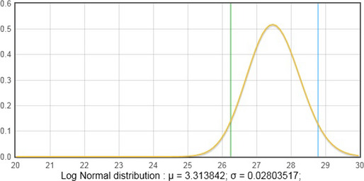
(Calculated with the MATCH elicitation tool, ref: David E. Morris, Jeremy E. Oakley, John A. Crowe, A web‐based tool for eliciting probability distributions from experts, Environmental Modelling and Software, Volume 52, February 2014, Pages 1–4)

Strengths

1. This approach of uncertainty analysis could be used in situations where other methods are not applicable due to restricted empirical data, literature, other evidence, or due to limited resources.

2. The essential elements of the EKE reduce the impact of known psychological problems in eliciting expert judgements and ensure a transparent documentation and complete reasoning.

3. Using semi‐formal EKE will it be possible to express uncertainties in a quantitative manner, e.g. by probability distributions, in almost all situations.

Weaknesses and possible approaches to reduce them

1. Even when this approach is able to identify and quantify uncertainties, it is not able to increase the evidence from data, e.g. experiments/surveys and literature.

2. EKE is not a substitute for data. Rather, it provides a rigorous and transparent way to express what is known about a parameter from existing evidence, and can provide a good basis for deciding whether to request additional data.

3. In comparison to the formal EKE, the definition of the question, the selection of the expert board and the performance of the elicitation protocol are restricted to the competencies in the Working Group.

4. No internal, independent review is foreseen to validate the quality of the elicitation, and finally the result.

Assessment against evaluation criteria

This method is assessed against the criteria in Table B.15.

Conclusions

1. The method has a high applicability in Working Groups and boards of EFSA and should be applied to quantify uncertainties in all situations:

   1. where empirical data from experiments/surveys, literature are limited;

   2. where the purpose of the risk assessment does not require the performance of a full formal EKE;

   3. or where restrictions in the resources (e.g. in urgent situations) forces EFSA to apply a simplified procedure.

2. The method is applicable in all steps of the risk assessment, esp. to summarise the overall uncertainty of the conclusion. Decisions on the risk assessment methods (e.g. risk models, factors, sources of uncertainties) could be judged qualitatively with quantitative elements (e.g. subjective probabilities on appropriateness, what‐if scenarios).

3. The method should not substitute the use of empirical data, experiments, surveys or literature, when these are already available or could be retrieved with corresponding resources.

4. In order to enable an EFSA Working Group to perform expert elicitations, all experts should have basic knowledge in probabilistic judgements and some experts of the Working Group should be trained in steering expert elicitations according to the EFSA Guidance.

5. Detailed guidance for semi‐formal EKE should be developed to complement the existing guidance for formal EKE (EFSA, 2014a,b), applicable to a range of judgement types (quantitative and categorical questions, approximate probabilities, probability bounds, etc.).

References

EFSA (European Food Safety Authority), 2014. Guidance on Expert Knowledge Elicitation in Food and Feed Safety Risk Assessment. EFSA Journal 2014;12(6):3734. https://doi.org/10.2903/j.efsa.2014.3734

Morgan MG and Henrion M, 1990. Uncertainty – A Guide to dealing with uncertainty in quantitative risk and policy analysis. Cambridge University Press (UK), 1990.

Table B.18.

Assessment of Semi‐formal expert knowledge elicitation (when applied well) against evaluation criteria

Criteria	Evidence of current acceptance	Expertise needed to conduct	Time needed	Theoretical basis	Degree/extent of subjectivity	Method of propagation	Treatment of uncertainty and variability	Meaning of output	Transparency and reproducibility	Ease of understanding for non‐specialist
Stronger characteristics	International guidelines or standard scientific method	No specialist knowledge required	Hours	Well established, coherent basis for all aspects	Judgement used only to choose method of analysis	Calculation based on appropriate theory	Different types of uncertainty & variability quantified separately	Range and probability of possible answers	All aspects of process and reasoning fully documented	All aspects fully understandable
	EU level guidelines or widespread in practice	Can be used with guidelines or literature	Days	Most but not all aspects supported by theory	Combination of data and expert judgement	Formal expert judgement	Uncertainty and variability quantified separately	Range and relative possibility of answers	Most aspects of process and reasoning well documented	Outputs and most of process understandable
	National guidelines, or well established in practice or literature	Training course needed	Weeks	Some aspects supported by theory	Expert judgement on defined quantitative scales	Informal expert judgement	Uncertainty and variability distinguished qualitatively	Range of answers but no weighting	Process well documented but limited explanation of reasoning	Outputs and principles of process understandable
	Some publications and/or regulatory practice	Substantial expertise or experience needed	A few months	Limited theoretical basis	Expert judgement on defined ordinal scales	Calculation or matrices without theoretical basis		Quantitative measure of degree of uncertainty	Limited explanation of process and/or basis for conclusions	Outputs understandable but not process
Weaker characteristics	Newly developed	Professional statistician needed	Many months	Pragmatic approach without theoretical basis	Verbal description, no defined scale	No propagation	No distinction between variability and uncertainty	Ordinal scale or narrative description for degree of uncertainty	No explanation of process or basis for conclusions	Process and outputs only understandable for specialists

B.9. Formal process on Expert Knowledge Elicitation (EKE) as described in the corresponding EFSA Guidance

This section summarises the process on Expert Knowledge Elicitation (EKE) which is fully described and discussed in the corresponding EFSA Guidance (EFSA, 2014a,b). Because the Guidance focusses mainly on fully formal elicitation of important quantitative parameters in EFSA's risk assessments, a semi‐formal approach is described in Annex B.8. The EFSA (2014a,b) Guidance also describes a process of ‘minimal assessment’, which can be used to prioritise parameters for formal or semi‐formal EKE. Between the semi‐formal and formal EKE is a continuum of alternatives, which could be used to fit the process to the specific needs of the problem, e.g. reframe the problem into the language of practitioners – as described in the formal EKE – but using an existing network of experts – as described in the semi‐formal EKE.

Purpose, origin and principal features

Formal techniques for eliciting knowledge from specialised persons were introduced in the first half of the 20th century (e.g. Delphi method in 1946 or Focus groups in 1930 – Ayyub Bilal, 2001) and after the sixties they became popular in risk assessments in engineering (EFSA, 2014a,b).

Since then, several approaches were further developed and optimised. Regarding the individual expert judgement on uncertainties of a quantitative parameter, the use of subjective probabilities is common.

Nevertheless, alternatives exist like fuzzy logic (Zimmermann, 2001), belief functions (Shafer, 1976), imprecise probabilities (Walley, 1991) and prospect theory (Kahneman and Tversky, 1979). The authors claim that these concepts better represent the way experts think about uncertainties than the formal concept of probabilities. On the other hand, probabilities have a clear and consistent interpretation. They are therefore proposed in the EFSA Guidance on EKE (EFSA, 2014a,b).

Formal techniques describe the full process of EKE beginning with its initiation (problem definition) done by the Working Group, the pre‐elicitation phase (protocol definition: framing the problem, selecting the experts and method) done by a steering group, the main elicitation phase (training and elicitation) done by the elicitation group and the post‐elicitation phase (documentation) as common task.

Each phase has a clearly defined output which will be internally reviewed and passed to the next phase. The Working Group is responsible to define the problem to be elicited, summarise the risk assessment context and the existing evidence from empirical data and literature. The steering group will develop the elicitation protocol from the question by framing the problem according to the intended expert board, selecting the experts for the elicitation and the elicitation method to be applied. Finally, the elicitation group will perform the elicitation and analyse the results. The separation of the elicitation from the Working Group allows EFSA to outsource the elicitation to an external contractor with professional experience in the selected elicitation method, to guarantee full confidentiality to the board of external experts, and third to enable the Working Group to perform an independent review of the results.

Figure B.6.

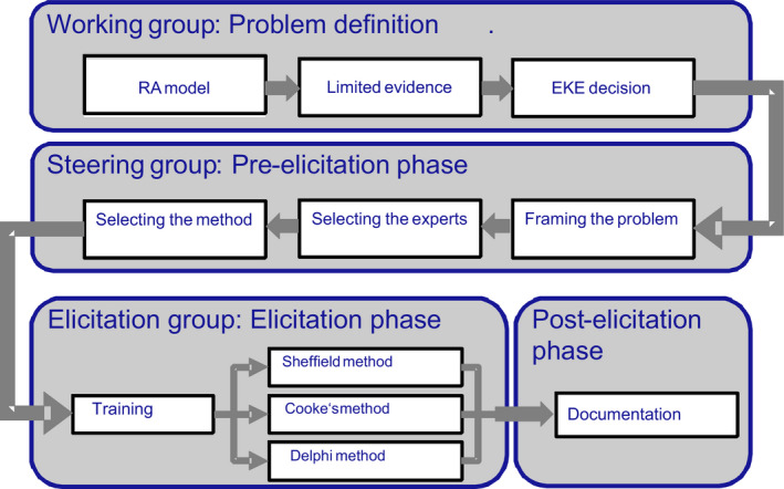
The process of expert knowledge elicitation (EFSA, 2014a)

The elicitation methods differ in the way the judgements of several experts are aggregated. In general three types of methods can be distinguished:

1. Behavioural aggregation: Individual judgements will be aggregated by group interaction of the experts, e.g. using the Sheffield method (O'Hagan et al., 2006).

2. Mathematical aggregation: Individual judgements will be aggregated by a weighted average using, e.g. seed questions to calibrate the experts, e.g. the Cooke method (Cooke, 1991).

3. Mixed methods: Individual judgements will be aggregated by moderated feedback loops avoiding direct interactions in the group, e.g. the Delphi protocol as described in EFSA (2014a,b).

The result is in all methods a probability distribution describing the uncertainty of a quantitative parameter in risk assessment, like an influencing factor or the final risk estimate.

Detailed discussion of the principles of EKE and step‐by‐step guidance and examples for the three methods mentioned above are provided by EFSA (2014a,b). The protocols in EFSA (2014a) can be applied to judgements about uncertain variables, as well as parameters, if the questions are framed appropriately (e.g. eliciting judgements on the median and the ratio of a higher quantile to the median). EFSA (2014a,b) does not address other types of judgements needed in EFSA assessments, including prioritising uncertainties and judgements about dependencies, model uncertainty, categorical questions, approximate probabilities and probability bounds. More guidance on these topics, and on the elicitation of uncertain variables, would be desirable in future.

Applicability in areas relevant for EFSA

Formal EKE is applicable in all areas where empirical data from experiments/surveys or literature are limited or missing, and theoretical reasoning is not available, e.g. on future, emerging risks. It is an additional alternative to involve a broad range of stakeholders. In complex, ambiguous risk assessments it is also a possibility to pass the elicitation of detailed questions to independent institutions to gather evidence in broader communities of expertise.

Potential contribution to major elements of uncertainty analysis

Elements in uncertainty analysis	Potential contribution of this approach
Identifying uncertainties	No, question must be defined beforehand
Characterising uncertainties	Yes, by a clearly defined process
Combining uncertainties	Yes, by a clearly defined process
Prioritising uncertainties	No

Melamine example

The following hypothetical example was constructed to illustrate the approach. The problem was divided into two parts: The determination of upper and lower limits for the fraction of milk power [dry milk solids in %], which can be used to produce saleable milk chocolate (without unacceptable changes in taste, consistence or other features of the chocolate). These are handled in questions 1 and 2. And finally the variation in the fraction of milk powder [dry milk solids in %] in chocolate imported from China. For the final third question a different board of experts was defined.

Question 1: What is the maximum fraction of milk power [dry milk solids in %], which can be used to produce saleable milk chocolate (without unacceptable changes in taste, consistence or other features of the chocolate)?

Question 2: What is the minimum fraction of milk power [dry milk solids in %], which have to be used to produce saleable milk chocolate (without unacceptable changes in taste, consistence or other features of the chocolate)?

Experts to ask:

Profile: Product developers in big chocolate production companies (including milk chocolate products)

Number of experts: 2–3, because of standardised production processes.

Elicitation methods: Written procedure using the adapted Delphi approach. This approach is asking the experts to describe their uncertainty by five numbers:

Steps	Parameter	Explanation
Procedure		To avoid psychological biases in estimating quantitative parameters please give the requested numbers in the right queueing:
1st step:	Upper (U)	Upper limit of uncertainty of the maximum fraction of milk powder in saleable chocolate:‘You should be really surprised, when you would identify a chocolate with a fraction of milk powder above the upper limit on the market’.
2nd step:	Lower (L)	Lower limit of uncertainty of the maximum fraction of milk powder in saleable chocolate:‘You should be really surprised, when a person is claiming that a chocolate with a fraction of milk powder below the lower limit is not saleable because of too high milk powder content’.
3rd step:	Median (M)	Median (or second quartile of uncertainty) of the maximum fraction of milk powder in saleable chocolate:‘Regarding your uncertainty about the true answer this is your best estimate of the maximum fraction of milk powder in saleable chocolate: in the sense that if you would get the true answer (by a full study/experiment) it is equal likely that the true value is above the median (M ≤ true value ≤ U) as it is below the median (L ≤ true value ≤ M)’.
4th step:	3rd quartile (Q3)	Third quartile of uncertainty of the maximum fraction of milk powder in saleable chocolate: ‘Assuming that the true answer is above the median this is the division of the upper interval (between median and the upper limit: [M, U]) into two parts which are again equal likely: 1) between the median and the third quartile: [M, Q3] 2) between the third quartile and the upper limit: [Q3, U]’
5th step:	1st quartile (Q1)	First quartile of uncertainty of the maximum fraction of milk powder in saleable chocolate: ‘Assuming that the true answer is below the median this is the division of the upper interval (between lower limit and the median: [L, M]) into two parts which are again equal likely: 1) between the lower limit and the first quartile: [L, Q1] 2) between the first quartile and the median: [Q1, M]’
Restrictions:		The five numbers are ordered from low to high as: L ≤ Q1 ≤ M ≤ Q3 ≤ U
Consistency check:		Finally, please check if the following four intervals will have equal probability (of 25% or one quarter) to include the true maximum fraction of milk powder in saleable chocolate: 1) between the lower limit and the first quartile: [L, Q1] 2) between the first quartile and the median: [Q1, M] 3) between the median and the third quartile: [M, Q3] 4) between the third quartile and the upper limit: [Q3, U]This can be visualised by a bar chart on the four intervals, where each bar contains the same area of 25%, which is an expression of the subjective distribution of uncertainty.

First round with initial answers and reasoning (asked with a specific EXCEL file giving more explanations and setting restrictions to the answers) was performed during the first week involving three experts (hypothetical example for illustration):

• Mrs. White, Chocolate Research Inc. (UK);

• Mrs. Argent, Chocolatiers Unis (France);

• and Mr. Rosso, Dolce International (Italy).

	Lower	1st Quart	Median	3rd Quart	Upper	Reasoning
Expert no 1	24.5%	24.8%	25%	25.5%	26.5%	Variation in our production line of the product with highest content of milk power
Expert no 2	20%	24%	26%	27%	30%	Depending on the sugar content there will be an aftertaste of the milk powder
Expert no 3	27%	27.5%	28%	28.5%	29%	We recognised problems in the production line when higher the milk powder content

After feedback of the answers to the experts they revised in the second week their answers:

	Lower	1st Quart	Median	3rd Quart	Upper	Reasoning
Expert no 1	27.5%	27.8%	28%	28.5%	29.5%	Higher contents are possible, but not used by my company
Expert no 2	20%	24%	26%	27%	30%
Expert no 3	27%	27.5%	28%	28.5%	29%

As result of the procedure, the judgements of all three experts were combined by using equal weights to each expert.

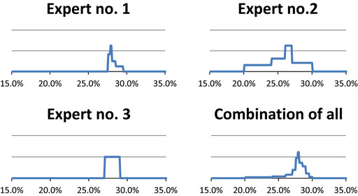
At the same time, the expert board was asked about the minimum content of milk powder in milk chocolate. The experts concluded that milk chocolate needs by legal requirements a minimum of 14% milk powder (dry milk solids obtained by partly or wholly dehydrating whole milk, semi‐ or full‐skimmed milk, cream, or from partly or wholly dehydrated cream, butter or milk fat; EC Directive 2000/36/EC, Annex 1, A4 of 23 June 2000). The risk assessment is therefore restricted to the consumption of chocolate following the legal requirements. Illegal trade (in this sense) is not included. The minimum was set to 14%.

To assess the variability of melamine content in chocolate imported from China, an additional Question 3 was asked to another board of experts:

Question 3: Assuming that milk chocolate was produced in and imported from China.

Part 3A: Consider a producer using a high content of milk powder in the chocolate that only in 5% (one of twenty) of the products from China will be with a higher content. What is the fraction of milk power [in %] contained in this chocolate? (Please specify your uncertainty)

Part 3B: Consider a producer using a low content of milk powder in the chocolate that only in 5% (one of twenty) of the products from China will be with a lower content. What is the fraction of milk power [in %] contained in this chocolate? (Please specify your uncertainty)

Part 3C: Consider a producer using an average content of milk powder in the chocolate that half of the products from China will be with higher and half with lower content. What is the fraction of milk power [in %] contained in this chocolate? (Please specify your uncertainty)

Experts to ask:

Profile: Quality controller (laboratory) of food importing companies/food control in importing regions with relevant import of chocolate or similar products (containing milk powder) from China.

Number of experts: 4, because of the limited number of experts with this profile.

Elicitation methods (hypothetical example): The expert board was invited to a one‐day physical meeting, summarising the identified evidence on the topic. After a training session on the elicitation method, the Sheffield protocol was performed on Question 3, parts A–C.

Strengths

1. Applicable in the absence of empirical data or theoretical reasoning.

2. Reproducible with regard to the predefined protocol.

3. Transparent in the documentation.

4. Applicable for emerging (future) risks/participation of stakeholders in complex, ambiguous RA.

Weaknesses and possible approaches to reduce them

1. Time and resource intensive, should be primarily used for the most sensitive parameters in a risk assessment.

2. Little previous experience of this approach in EFSA's areas of risk assessment. However, there is a substantial literature by expert practitioners, and it is better established in other areas (e.g. nuclear engineering, climate change).

Assessment against evaluation criteria

This method is assessed against the criteria in Table B.19.

Table B.19.

Assessment of Formal expert knowledge elicitation (EKE) (when applied well) against evaluation criteria

Criteria	Evidence of current acceptance	Expertise needed to conduct	Time needed	Theoretical basis	Degree/extent of subjectivity	Method of propagation	Treatment of uncertainty and variability	Meaning of output	Transparency and reproducibility	Ease of understanding for non‐specialist
Stronger characteristics	International guidelines or standard scientific method	No specialist knowledge required	Hours	Well established, coherent basis for all aspects	Judgement used only to choose method of analysis	Calculation based on appropriate theory	Different types of uncertainty & variability quantified separately	Range and probability of possible answers	All aspects of process and reasoning fully documented	All aspects fully understandable
	EU level guidelines or widespread in practice	Can be used with guidelines or literature	Days	Most but not all aspects supported by theory	Combination of data and expert judgement	Formal expert judgement	Uncertainty and variability quantified separately	Range and relative possibility of answers	Most aspects of process and reasoning well documented	Outputs and most of process understandable
	National guidelines, or well established in practice or literature	Training course needed	Weeks	Some aspects supported by theory	Expert judgement on defined quantitative scales	Informal expert judgement	Uncertainty and variability distinguished qualitatively	Range of answers but no weighting	Process well documented but limited explanation of reasoning	Outputs and principles of process understandable
	Some publications and/or regulatory practice	Substantial expertise or experience needed	A few months	Limited theoretical basis	Expert judgement on defined ordinal scales	Calculation or matrices without theoretical basis		Quantitative measure of degree of uncertainty	Limited explanation of process and/or basis for conclusions	Outputs understandable but not process
Weaker characteristics	Newly developed	Professional statistician needed	Many months	Pragmatic approach without theoretical basis	Verbal description, no defined scale	No propagation	No distinction between variability and uncertainty	Ordinal scale or narrative description for degree of uncertainty	No explanation of process or basis for conclusions	Process and outputs only understandable for specialists

Conclusions

1. The method has a high applicability in Working Groups and boards of EFSA and should be applied to quantify uncertainties in situations where empirical data from experiments/surveys, literature are limited and the purpose of the risk assessment is sensitive and need the performance of a full formal EKE.

2. The method is applicable in steps of the risk assessment, where quantitative parameters have to be obtained.

3. The method should not substitute the use of empirical data, experiments, surveys or literature, when these are already available or could be retrieved with corresponding resources.

4. In order to initiate a formal EKE, some experts of the Working Group should be trained in steering expert elicitations according to the EFSA Guidance. In case of complex or sensitive questions, the elicitation should be performed by professional elicitation groups.

5. Further guidance is needed on formal methods for types of expert elicitation not covered by EFSA (2014a,b) (e.g. for variables, dependencies, qualitative questions, approximate probabilities and probability bounds), as well as on semi‐formal methods.

References

Cooke RM, 1991. Experts in uncertainty. Oxford University Press, Oxford, UK.

EFSA (European Food Safety Authority), 2014. Guidance on Expert Knowledge Elicitation in Food and Feed Safety Risk Assessment. EFSA Journal 2014;12(6):3734. [278 pp.] https://doi.org/10.2903/j.efsa.2014.3734

O'Hagan A, Buck CE, Daneshkhah A, Eiser JR, Garthwaite PH, Jenkinson D, Oakley JE and Rakow T, 2006. Uncertain judgements: eliciting experts’ probabilities. John Wiley and Sons, Chichester, UK.

Shafer G, 1976. A mathematical theory of evidence. Princeton University Press, Princeton, NJ, USA.

Zimmermann HJ, 2001. Fuzzy set theory—and its applications, 4th edn. Springer, New York, USA.

B.10. Confidence intervals

This section is only concerned with standard calculations for confidence intervals. The bootstrap is discussed in a separate section of this annex (Annex B.11).

Purpose, origin and principal features

A confidence interval is the conventional expression of uncertainty, based on data, about a parameter in a statistical model. The basic theory (Cox, 2006) and methodology was developed by statisticians during the first half of the 20th century. Confidence intervals are used by the majority of scientists as a way of summarising inferences from experimental data and the training of most scientists includes some knowledge of the underlying principles and methods of application. See, for example, Moore (2009).

A confidence interval provides a range of values for the parameter together with a level of confidence in that range (commonly 95% or 99%). Formally, the confidence level indicates the success rate of the procedure under repeated sampling and assuming that the statistical model is correct. However, the confidence level is often interpreted for a specific data set, as the probability that the calculated range actually includes the true value of the parameter, i.e. a 95% confidence interval becomes a 95% credible interval for the parameter. That interpretation is reasonable in many cases but requires for each specific instance that the user of the confidence interval make a judgement that it is a reasonable interpretation. This is in contrast to Bayesian inference (Annex B.9) which sets out to produce credible intervals from the outset. The judgement the user needs to make is that they do not have additional information which would make them want to alter the probability to be ascribed to the interval (see Section 11.2.1 for more detail on this issue).

To use this method, one requires a suitable statistical model linking available data to parameters of interest and an appropriate procedure for calculating the confidence interval. For many standard statistical models, such procedures exist and are often widely known and used by scientists. Developing new confidence interval calculations is generally a task for theoretical statisticians.

Many standard confidence interval procedures deliver only an approximation to the stated level of confidence and the accuracy of the approximation is often not known explicitly although it usually improves as the sample size increases. When the statistical model does not correctly describe the data, the confidence level is affected, usually by an unknown amount.

Most statistical models have more than one parameter and in most cases the resulting uncertainty about the parameters will involve dependence. Unless there is very little dependence, it is inappropriate to express the uncertainty as a separate confidence interval for each parameter. Instead, the uncertainty should be expressed as a simultaneous confidence region for all the parameters. An example of such a method, which achieves the stated confidence level exactly, is the rarely used joint confidence region for the mean and standard deviation of a normally distributed population based on random sample. Approximate methods exist for confidence regions for a wide variety of statistical models, based on large sample behaviour of maximum likelihood estimation. Such methods are often technically challenging for non‐statisticians and it may be preferable in practice to use another statistical approach to representing uncertainty, especially one which can represent uncertainty as a Monte Carlo sample, each realisation of which provides a value for each of the parameters.

Applicability in areas relevant for EFSA

The methodology is applicable in principle to all areas where data from experiments or surveys are used in risk assessment.

However, unless data are being used to make inference about a single parameter of interest in statistical model, addressing dependence between parameters is likely to be challenging and this may reduce the usefulness of confidence intervals as an expression of uncertainty.

Standard confidence interval procedures, such as those for means of populations, regression coefficients and dose–response estimates, are used throughout EFSA's work.

Potential contribution to major elements of uncertainty analysis

Elements in uncertainty analysis	Potential contribution of this approach
Identifying uncertainties	Not applicable
Characterising uncertainties	Yes/No. Limited to uncertainties relating to parameters in statistical models. For many statistical models, there is a clear procedure based on empirical data
Combining uncertainties	Not applicable
Prioritising uncertainties	Not applicable

Melamine example

Confidence intervals and regions will be illustrated by application to uncertainty about two of the sources of variability considered in the version of the melamine example which considers uncertainty about variability of exposure. Further supporting details about both versions of the melamine example may be found in Annex C. The variables considered here are body weight and consumption in a day.

Data for both variables for children aged from 1 up to 2 years old were obtained from EFSA. Annex C gives details of the data and some data analysis supporting the choice of distribution family for each variable. The variables are treated as independent in what follows and the reasoning for doing so is included in Annex C.

Both variables are considered in detail below because there are important differences between the statistical models used. The normal distribution used for log body weight is the most commonly used model for continuous variability and the confidence interval procedures are well known. The gamma distribution used for consumption requires more advanced statistical calculations and also shows the importance of addressing dependence between distribution parameters.

Body weight (bw)

For bw, the statistical model is that: (i) bw follows a log‐normal distribution, so that log bw follows a normal distribution; (ii) the uncertain distribution parameters are the mean ${\mathrm{\mu }}_{log\mathrm{bw}}$ and standard deviation σ_logbw of the distribution of log bw (base 10); (iii) the data are a random sample from the distribution of bw for the population represented by the data.

For the mean and standard deviation of a normal distribution, there are standard confidence interval procedures which assume that the data are a random sample.

For the mean the confidence interval is $\overline{\mathrm{x}}\pm \mathrm{t}\times \mathrm{s}/\sqrt{\mathrm{n}}$ where $\mathrm{\beta }x$ denotes the sample mean, s is the sample standard deviation and n is the sample size. t* is a percentile of the t‐distribution having n−1 degrees of freedom. The percentile to be chosen depends on the confidence level: for example, for 95% confidence, it is the 97.5th percentile; for 99% confidence, the 99.5th percentile. For the standard deviation, the confidence interval is $(\mathrm{s}/\sqrt{{\mathrm{\chi }}_{\mathrm{u}}^2(\mathrm{n}-1)},\mathrm{s}/\sqrt{{\mathrm{\chi }}_{\mathrm{l}}^2/(\mathrm{n}-1)})$ where again s is the sample standard deviation and n is the sample size. ${\chi }_l^2$ and ${\chi }_u^2$ are lower and upper percentiles of the chi‐squared distribution having n−1 degrees of freedom. The percentiles to be used depend on the required confidence level: for example, for 95% confidence, they are the 2.5th and 97.5th percentiles. Values for $t^{\ast },{\mathrm{\chi }}_{\mathrm{l}}^2$ and ${\mathrm{\chi }}_{\mathrm{u}}^2$ are easily obtained from tables or using standard statistical software.

For the body weight data used in the example, n_lobbw = 171,  ${\overline{\mathrm{x}}}_{\mathrm{lobbw}}=1.037,$ and s_lobbw = 0.060. Taking 95% as the confidence level, t* = 1.974,  ${\mathrm{\chi }}_{\mathrm{l}}^2=135.79$ and ${\mathrm{\chi }}_{\mathrm{u}}^2=208.00.$ Consequently, the confidence interval for μ_logbw is $1.037\pm 1.974\times 0.060/\sqrt{171}=1.037\pm 0.009=(1.028,1.046)$ and the confidence interval for σ_logbw is $(0.060/\sqrt{208.00/170},0.060\sqrt{135.79/170})=(0.054,0.067).$

Because the mean of the underlying normal distribution is the logarithm of the geometric mean (and median) of a log‐normal, we can convert the confidence interval for μ_logbw into a 95% confidence interval for the geometric mean of body weight: (10^1.028, 10^1.046) = (10.67, 11.12) kg. Similarly, the standard deviation of the underlying normal is the logarithm of the geometric standard deviation of the log‐normal and so a 95% confidence interval for the geometric standard deviation of body weight is (10^0.054, 10^0.067) = (1.13, 1.17).

Each of these confidence intervals is an expression of uncertainty about the corresponding uncertain parameter for variability of body weight. However, they do not express that uncertainty in a form which is directly suitable for use in a probability bounds analysis or Monte Carlo uncertainty analysis. In the absence of further information about body weight, experts may be willing to make a probabilistic interpretation of the confidence level, as explained in the opening section of this annex.

In principle, given data, there is dependence in the uncertainty about the two parameters of a normal distribution. That dependence may be substantial when the sample size is small but decreases for larger samples.

Consumption (q)

For q, the statistical model is that: (i) q follows a gamma distribution with uncertain distribution parameters being the shape α_q and rate β_q; (ii) the data are a random sample from the distribution of q.

Like the normal and log‐normal distributions, the gamma family of distributions has two distribution parameters. The most common choice of how to parameterise the distribution is the mathematically convenient one of a shape parameter α and a rate parameter β so that the probability density for q is $\mathrm{p}(\mathrm{q})\infty \frac{{\mathrm{\beta }}^{\mathrm{\alpha }}}{\mathrm{\tau }(\mathrm{\alpha })}{\mathrm{q}}^{\mathrm{\alpha }-1}{\mathrm{e}}^{-\mathrm{\beta }\mathrm{q}}.$

There are a number of ways to get approximate confidence intervals for both distribution parameters. Of those, the one which has the best performance is maximum likelihood estimation (Whitlock and Schluter, 2014) combined with large sample approximation confidence interval calculations. However, the main practical difficulty is that the sampling distributions of estimates of the parameters are strongly correlated and so it is not very useful to consider uncertainty about each parameter on its own. The large sample theory for maximum likelihood estimation shows how to compute a simultaneous confidence region for both parameters. Figure B.7 shows the maximum likelihood estimate and 95% and 99% confidence regions for α and β based the consumption data used in the example; the dotted vertical and horizontal lines show, respectively, the ends of the 95% confidence intervals for α and β.

Figure B.7.

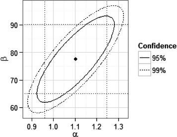
Confidence regions for distribution parameters for gamma distribution used to model variability of consumption by 1‐year‐old children

Strengths

1. For many survey designs or study designs and corresponding statistical models, there is familiar methodology to obtain confidence intervals for individual statistical model parameters.

2. Widely available software for computing confidence intervals (Minitab, R, Systat, Stata, SAS, etc.)

3. Computations are based on the generally accepted mathematical theory of probability although probability is only used directly to quantify variability.

Weaknesses and possible approaches to reduce them

1. Confidence intervals only address uncertainties relating to parameters in statistical models.

2. Requires specification of a statistical model for data, the model depending on parameters which be estimated. Specifying and fitting non‐standard models can be time‐consuming and difficult for experts and may often require the involvement of a professional statistician.

3. Results are expressed in the language of confidence rather than of probability. Uncertainties expressed in this form can only be combined in limited ways. They can only be combined with probabilistic information if experts are willing to make probability statements on the basis of their knowledge of one or more confidence intervals.

4. Dependence in the uncertainties about statistical model parameters is usual when a statistical model having more than one parameter is fitted to data. This can be addressed in principle by making a simultaneous confidence statement about multiple parameters. However, such methods are much less familiar to most scientists and generally require substantial statistical expertise.

Assessment against evaluation criteria

This method is assessed against the criteria in Table B.20.

Table B.20.

Assessment of Confidence intervals (when well applied) against evaluation criteria

Criteria	Evidence of current acceptance	Expertise needed to conduct	Time needed	Theoretical basis	Degree/extent of subjectivity	Method of propagation	Treatment of uncertainty and variability	Meaning of output	Transparency and reproducibility	Ease of understanding for non‐specialist
Stronger characteristics	International guidelines or standard scientific method	No specialist knowledge required	Hours	Well established, coherent basis for all aspects	Judgement used only to choose method of analysis	Calculation based on appropriate theory	Different types of uncertainty & variability. quantified separately	Range and probability of possible answers	All aspects of process and reasoning fully documented	All aspects fully understandable
	EU level guidelines or widespread in practice	Can be used with guidelines or literature	Days	Most but not all aspects supported by theory	Combination of data and expert judgement	Formal expert judgement	Uncertainty and variability quantified separately	Range and relative possibility of answers	Most aspects of process and reasoning well documented	Outputs and most of process understandable
	National guidelines, or well established in practice or literature	Training course needed	Weeks	Some aspects supported by theory	Expert judgement on defined quantitative scales	Informal expert judgement	Uncertainty and variability distinguished qualitatively	Range of answers but no weighting	Process well documented but limited explanation of reasoning	Outputs and principles of process understandable
	Some publications and/or regulatory practice	Substantial expertise or experience needed	A few months	Limited theoretical basis	Expert judgement on defined ordinal scales	Calculation or matrices without theoretical basis		Quantitative measure of degree of uncertainty	Limited explanation of process and/or basis for conclusions	Outputs understandable but not process
Weaker characteristics	Newly developed	Professional statistician needed	Many months	Pragmatic approach without theoretical basis	Verbal description, no defined scale	No propagation	No distinction between variability and uncertainty	Ordinal scale or narrative description for degree of uncertainty	No explanation of process or basis for conclusions	Process and outputs only understandable for specialists

Conclusions

1. Confidence intervals are suitable for application across EFSA in situations where standard statistical models are used in order to quantify uncertainty separately about individual statistical model parameters using intervals.

2. The quantification provided is not directly suitable for combining with other uncertainties in probabilistic calculations although expert judgement may be applied in order to support such uses.

References

Cox DR, 2006. Principles of Statistical Inference. Cambridge University Press.

Moore DS, 2009. The Basic Practice of Statistics, 5th ed. WH Freeman.

Whitlock M and Schulter D, 2014. The Analysis of Biological Data, 2nd ed. Roberts and Company Publishers.

B.11. The bootstrap

B.11.1.

B.11.1.1.

Purpose, origin and principal features

The bootstrap is a tool for quantifying uncertainty due to sampling variability. It is both a basic sensitivity analysis tool and a method for producing approximate confidence intervals. It has the advantage that it is often easy to implement using Monte Carlo (see Annex B.14).

The bootstrap was originally proposed by Efron (1981). Davison and Hinkley (1997) give an account of theory and practice aimed at statisticians while Manly (2006) is aimed more at biologists and other scientists.

The problem it addresses is that it is usually uncertain how much the result of a calculation based on a sample of data might differ from the result which would be obtained by applying the calculation to the statistical population from which the data were drawn. For some statistical models, there is a well‐known mathematical solution to that problem. For others, there is not. The bootstrap provides an approximate answer which is often relatively easily calculated. The underlying principle is that, for many situations, sampling variability when sampling from the statistical population is similar to sampling variability when resampling from the data. It is often easy to resample from the data and repeat the calculation. By repeating the resampling process many times, it is possible to quantify the uncertainty attached to the original calculation.

The bootstrap can be applied in many ways and to a wide variety of parametric and non‐parametric statistical models. However, it is most easily applied to situations where data are a random sample or considered to be equivalent to a random sample. In such situations, the uncertainty attached to any statistical estimator(s) calculated from the data can be examined by repeatedly resampling from the data and repeating the calculation of the estimator(s) for each new sample. The estimator may be something simple like the sample mean or median or might be something much more complicated such as a percentile of exposure from estimated from data on consumption and concentrations. The resampling procedure is to take a random sample from the data, with replacement and of the same size as the data. Although from a theoretical viewpoint it is not always necessary, in practice the bootstrap is nearly always implemented using Monte Carlo sampling.

When applying an estimator to a particular data set, one is usually trying to estimate the population value: the value which would have been obtained by applying the estimator to the statistical population from which the data were drawn. There are many approaches to obtaining an approximate confidence interval, quantifying uncertainty about the population value, based on bootstrap output. The differences originate in differing assumptions about the relationship between resampling variability and sampling variability, some attempting to correct for potential systematic differences between sampling and resampling. All the approaches assume that the sample size is large. Further details are provided by Davison and Hinkley (1997).

The bootstrap can be used in relation to either a parametric or non‐parametric statistical model of variability. The advantage of the latter is that no parametric distribution family need be assumed but it has the potential disadvantage that, if the whole distribution is being used in any subsequent calculation, the only values which will be generated for the variable are those in the original data sample. The advantage of working with a parametric statistical model is that, if one bootstraps estimates of all the parameters, one obtains an indication of uncertainty about all aspects of the distribution.

The bootstrap will not perform well when the sample size is low or is effectively low. One example of an effectively low sample size would be when estimating non‐parametrically a percentile near the limit of what could be estimated from a given sample size. Another would be when a large percentage of the data take the same value, perhaps as values below a limit of detection or limit of quantification.

One very attractive feature of the bootstrap is that it can readily be applied to situations where there is no standard confidence interval procedure for the statistical estimator being used. Another is that it is possible to bootstrap more than one variable at the same time: if the data for two variables were obtained independently, then one takes a resample from each data set in each resampling iteration. The frequency property of any resulting confidence interval is then with respect to repetition not of a single survey/experiment but is with respect to repeating all of them.

Because the output of the bootstrap is a sample of values for parameters, it is computationally straightforward to use the output as part of a 2D Monte Carlo analysis (Annex B.14) of uncertainty. Such an analysis could use bootstrap output for some uncertainties and distributions obtained by EKE and/or Bayesian inference for other uncertainties. However, the meaning of the output of the Monte Carlo calculation is unclear unless an expert judgement has been made that the bootstrap output is a satisfactory probabilistic representation of uncertainty for the parameters on the basis of the data to which the bootstrap has been applied.

Applicability in areas relevant for EFSA

The bootstrap is a convenient way to make an assessment of uncertainty due to sampling variability in situations which involve a random sample of data and where it is difficult to calculate a standard confidence interval or make a Bayesian inference. As such, it has particular applicability to data obtained from random surveys which are used in complex statistical calculations, for example, estimation of percentiles of exposure using probabilistic modelling.

The bootstrap has been recommended as part of the EFSA (2012a,b,c) guidance on the use of probabilistic methodology for modelling dietary exposure to pesticide residues. However, that guidance recognises the limitations of the bootstrap and recommends that it be used alongside other methods. Bootstrapping was used frequently in microbial dose–response assessment but it has now largely been replaced by Bayesian inference (e.g. Medema et al., 1996; Teunis PFM et al., 1996).

Potential contribution to major elements of uncertainty analysis

Elements in uncertainty analysis	Potential contribution of this approach
Identifying uncertainties	Not applicable
Characterising uncertainties	Yes/No. Quantifies sampling variability but not other types of uncertainty
Combining uncertainties	No/Yes. Can be used to address multiple sources of uncertainty due to sampling variability in a single Monte Carlo calculation, thereby providing the combined impact of those, but not other, sources of uncertainty
Prioritising uncertainties	Not applicable

Melamine example

The bootstrap will be illustrated by application to uncertainty about one of the sources of variability considered in the version of the melamine example which considers uncertainty about variability of exposure. Further supporting details about both versions of the melamine example may be found in Annex C. The variable considered here is body weight. The body weight example is followed by a short discussion of the potential to apply the bootstrap to consumption: the other variable for which sample data were available.

Body weight (bw)

Data for body weight for children aged from 1 up to 2 years old were obtained from EFSA. Annex C gives details of the data and some data analysis supporting the choice of distribution family.

For bw, the statistical model is that: (i) bw follows a log‐normal distribution, so that log bw follows a normal distribution; (ii) the uncertain distribution parameters are the mean μ_logbw and standard deviation σ_logbw of the distribution of log bw (base 10); (iii) the data are a random sample from the distribution of bw for the population represented by the data.

First, consider uncertainty attached to the estimates of parameters for the log‐normal statistical model of variation in body weight. These parameters are the mean μ _logbw and standard deviation σ _logbw of log ₁₀ bw. They are estimated simply by calculating the sample mean and sample standard deviation of the observed data for log₁₀bw. Figure B.8 plots the values of these estimates for the original data and for 999 data sets resampled from the original data:

Figure B.8.

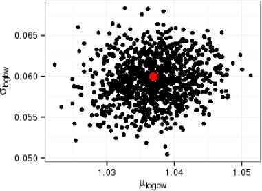
Estimates of parameters of log‐normal distribution fitted to data sets obtained by resampling the body weight data. The red point shows the estimates for the original data

The most commonly used methods for deriving a confidence interval from bootstrap output all give very similar answers for this example: an approximate 95% confidence interval for μ_logbw is (1.028, 1.046) and for σ_logbw the approximate 95% confidence interval using the ‘percentile’ method is (0.0540, 0.0652) while other methods give (0.0548, 0.0659). There are two reasons why different methods give very similar answers here: the original sample size is large and the mean and standard deviation are both estimators for which the bootstrap performs reasonable well.

If a specific percentile, say the 99th, of variability of body weight was of interest, there are two quite different approaches:

• For each bootstrap resample, the estimates of μ_logbw and σ_logbw can be calculated and then the estimated 99th percentile then μ_logbw + 2.33 * σ_logbw using the log‐normal model. Doing so provides 999 bootstrap values for the 99th percentile to which a bootstrap confidence interval calculation can be applied: the percentile method gives (1.158, 1.192) for 99th percentile of log₁₀bw which becomes (14.38, 15.56) as a CI for the 99th percentile of bw.

• Alternatively, the assumption of the log‐normal parametric statistical model can be dropped and a non‐parametric model for variability of body weight used instead. For each resampled data set, a non‐parametric estimate of the 99th percentile is computed and a bootstrap confidence interval calculation is then applied to the 999 values of the 99th percentile: the percentile method gives (14.00, 15.42) and other methods give somewhat slightly lower values for both ends of the confidence interval.

Other variables

The bootstrap cannot be applied to variability of concentration (c) or weight fraction (w) because no sample of data is available for either source of variability.

For consumption (q), the bootstrap could be applied. If uncertainty about the parameters alpha and beta of the gamma distribution model was required, it would be necessary to estimate the distribution parameters α_q and β_q for each resampled data set. This could be done by maximum likelihood estimation or, less optimally, by estimation using the method of moments.

Note that it would not be appropriate to carry out independent resampling of q and bw in this example. In the surveys from which the data were obtained, values for both variables come from the same individuals. The appropriate way to implement the bootstrap, to simultaneously address uncertainty about both q and bw, would be to resample entire records from the surveys. Doing so would also address dependence between q and bw.

Strengths

1. Computations are based on the generally accepted mathematical theory of probability although probability is only used directly to quantify variability.

2. Often does not require a lot of mathematical sophistication to implement.

3. Allows the user to decide what statistical estimator(s) to use.

4. Easily applied using Monte Carlo.

5. Specialist software exists for a number of contexts (CrystalBall, MCRA, Creme, etc.) as well as the possibility to use some general purpose statistical software, e.g. R.

Weaknesses and possible approaches to reduce them

1. The bootstrap only addresses random sampling uncertainty whereas other statistical inference methods can address a wider range of uncertainties affecting statistical models.

2. The performance of the bootstrap is affected both by the original sample size and by the estimator used. Larger samples generally improve the performance. Estimators which are not carefully designed may be badly biased or inefficient. This can be avoided by consulting a professional statistician.

3. The non‐parametric bootstrap never produces values in a resample which were not present in the data and consequently the tails of the distribution will be under‐represented.

4. Bootstrap confidence interval procedures are only approximate and in some situations the actual confidence may differ greatly from the claimed level. This can sometimes be ameliorated by carrying out a suitable simulation study.

5. Deciding when the method works well or badly often requires sophisticated mathematical analysis.

Assessment against evaluation criteria

This method is assessed against the criteria in Table B.21. The two extremes of the ‘Method of propagation’ column have both been selected because the method can combine uncertainties due to sampling variability for multiple variables but cannot combine those uncertainties with other kinds of uncertainty.

Table B.21.

Assessment of The bootstrap (when applied well) against evaluation criteria

Criteria	Evidence of current acceptance	Expertise needed to conduct	Time needed	Theoretical basis	Degree/extent of subjectivity	Method of propagation	Treatment of uncertainty and variability	Meaning of output	Transparency and reproducibility	Ease of understanding for non‐specialist
Stronger characteristics	International guidelines or standard scientific method	No specialist knowledge required	Hours	Well established, coherent basis for all aspects	Judgement used only to choose method of analysis	Calculation based on appropriate theory	Different types of uncertainty & variability quantified separately	Range and probability of possible answers	All aspects of process and reasoning fully documented	All aspects fully understandable
	EU level guidelines or widespread in practice	Can be used with guidelines or literature	Days	Most but not all aspects supported by theory	Combination of data and expert judgement	Formal expert judgement	Uncertainty and variability quantified separately	Range and relative possibility of answers	Most aspects of process and reasoning well documented	Outputs and most of process understandable
	National guidelines, or well established in practice or literature	Training course needed	Weeks	Some aspects supported by theory	Expert judgement on defined quantitative scales	Informal expert judgement	Uncertainty and variability distinguished qualitatively	Range of answers but no weighting	Process well documented but limited explanation of reasoning	Outputs and principles of process understandable
	Some publications and/or regulatory practice	Substantial expertise or experience needed	A few months	Limited theoretical basis	Expert judgement on defined ordinal scales	Calculation or matrices without theoretical basis		Quantitative measure of degree of uncertainty	Limited explanation of process and/or basis for conclusions	Outputs understandable but not process
Weaker characteristics	Newly developed	Professional statistician needed	Many months	Pragmatic approach without theoretical basis	Verbal description, no defined scale	No propagation	No distinction between variability and uncertainty	Ordinal scale or narrative description for degree of uncertainty	No explanation of process or basis for conclusions	Process and outputs only understandable for specialists

Conclusions

1. The bootstrap is suitable for application across EFSA in situations where data are randomly sampled and it is difficult to apply other methods of statistical inference.

2. It provides an approximate quantification of uncertainty in such situations and is often easy to apply using Monte Carlo.

3. The results of the bootstrap need to be evaluated carefully, especially when the data sample size is not large or when using an estimator for which the performance of the bootstrap has not been previously considered in detail.

References

Davison AC and Hinkley DV, 1997. Bootstrap Methods and their Application. Cambridge University Press.

Efron B, 1981. “Nonparametric estimates of standard error: The jackknife, the bootstrap and other methods”. Biometrika 68 (3), 589–599.

EFSA PPR Panel (Panel on Plant Protection Products and their Residues), 2012. Guidance on the Use of Probabilistic Methodology for Modelling Dietary Exposure to Pesticide Residues. EFSA Journal 2012;10(10):2839, 95 pp. https://doi.org/10.2903/j.efsa.2012.2839

Manly BFJ, 2006. Randomization, Bootstrap and Monte Carlo Methods in Biology, 3rd ed. Chapman and Hall/CRC.

Medema GJ, Teunis PF, Havelaar AH and Haas CN, 1996. Assessment of the dose‐response relationship of Campylobacter jejuni. Int J Food Microbiol 1996;30(1‐2):101‐11.

Teunis PFM, Van der Heijden OG, Van der Giessen JWB and Havelaar AH, 1996. The dose‐response relation in human volunteers for gastro‐intestinal pathogens. Bilthoven: National Institute of Public Health and the Environment, 1996 Report nr. 284550002.

B.12. Bayesian inference

B.12.1.

B.12.1.1.

Purpose, origin and principal features

Bayesian inference is a methodology for expressing and calculating uncertainty about parameters in statistical models, based on a combination of expert judgements and data. The resulting uncertainty is expressed as a probability distribution for the statistical model parameters and is therefore well‐suited for combining with other uncertainties using the mathematics of probability.

The principle underlying Bayesian inference has a long history in the theoretical development of statistical inference. However, it was not until the advent of modern computing that it started to be widely applied and new methodology developed. Since around 1990, there has been an explosion in Bayesian research and in application to all areas of natural and social sciences and to quantification of uncertainty in various financial sectors of business. Between them, Berry (1995), Kruschke (2010) and Gelman et al. (2013) cover a wide range from elementary Bayesian principles to advanced techniques.

It differs in two key features from other methods of statistical inference considered in this document. First, with Bayesian approaches, uncertainty about the parameter(s) in a statistical model is expressed in the form of a probability distribution so that not only a range of values is specified but also the probabilities of values. Second, the judgements of experts based on other information can be combined with the information provided by the data. In the language of Bayesian inference, those expert judgements must be represented as a prior distribution for the parameter(s). As for other expert judgements, they should be based on evidence and the experience of the expert (Section 5.9). The statistical model applied to the observed data provides the likelihood function for the parameter(s). The likelihood function encapsulates the information provided by the data. The prior distribution and likelihood function are then combined mathematically to calculate the posterior distribution for the parameter(s). The posterior distribution is the probabilistic representation of the uncertainty about the parameter(s), obtained by combining the two sources of information.

The prior distribution represents uncertainty about the values of the parameters in the model prior to observing the data. The prior distribution should preferably be obtained by expert knowledge elicitation (see Section 11.3 and Annexes B.8 and B.9). For some models, there exist standard choices of prior distribution which are intended to represent lack of knowledge. If such a prior is used, it should be verified that the statements it makes about the relative likelihood of different parameter values are acceptable to relevant experts for the parameter in question. It is a good idea in general to assess the sensitivity of the posterior distribution to the choice of prior distribution. If the output of the assessment is found to be sensitive to this choice, extra attention needs to be given to ensuring that the prior distribution represents the judgements of the expert(s). This is particularly important if a standard prior distribution was used.

The concept of credible interval (also sometimes known as a probability interval), an interval of values having a specified probability, based on the posterior distribution is sometimes seen as analogous to the concept of confidence interval in non‐Bayesian statistics. However, for a specified probability, there are many different ways to determine a credible interval from a posterior distribution and it is often better not to summarise the posterior in this way but to carry the full posterior distribution forward into subsequent probability calculations.

As with other methods of statistical inference, calculations are straightforward for some statistical models and more challenging for others. A common way of obtaining a practically useful representation of uncertainty is by a large random sample from the distribution, i.e. Monte Carlo (see Annex B.14). For some models, there is a simple way to perform Monte Carlo to sample from the posterior distribution; for others, it may be necessary to use some form of Markov Chain Monte Carlo. Markov Chain Monte Carlo is more complex to implement but has the same fundamental benefit that uncertainty can be represented by a large sample of possible values for the statistical model parameter(s).

If data are not available in raw form but only summaries are presented it may possible in some situations still to carry out a full Bayesian analysis. Exactly what is possible will depend on the model and on the detail of what summary information is provided. The same applies if only the results of a non‐Bayesian statistical analysis of the data are available.

Applicability in areas relevant for EFSA

It is applicable to any area where a statistical model with uncertain parameters is used as a model of variability. However, training in Bayesian statistics is not yet part of the standard training of scientists and so it will often be the case that some specialist assistance will be needed, for example, from a statistician.

EFSA Scientific Opinion and guidance documents have proposed the use of Bayesian methods for specific problems (EFSA, 2006; EFSA, 2012; EFSA, 2015a,b,c). They have also been applied in EFSA internal and external scientific reports (EFSA, 2009; Hald et al., 2012). However, at present, they are not widely used by EFSA.

The use of Bayesian methods has been proposed in many scientific articles concerning risk assessment in general and also those addressing particular applications. They have been adopted by some organisations for particular applications. For example, Bayesian methods have been used in microbial risk assessment by RIVM (Netherlands), USDA (USA) and IFR (UK) (Teunis and Havelaar, 2000). Bayesian methods are also widely used in epidemiology and clinical studies which are fields with close links to risk assessment (e.g. Teunis et al., 2008).

Potential contribution to major elements of uncertainty analysis

Elements in uncertainty analysis	Potential contribution of this approach
Identifying uncertainties	Not applicable
Characterising uncertainties	Yes. For each source, uncertainty is expressed as a probability distribution. Where there is dependence between uncertainties about two or more parameters, the joint uncertainty is expressed using a multivariate probability distribution
Combining uncertainties	Not applicable. However, the results of EKE and/or Bayesian inferences for multiple uncertainties may be combined using the mathematics of probability. This is seen by some as being part of an overarching Bayesian approach to uncertainty
Prioritising uncertainties	Not applicable. However, there exist methods of sensitivity analysis which are proposed from a Bayesian perspective and which are seen by some as being particularly appropriate for use in conjunction with Bayesian inference

Melamine example

Bayesian inference will be illustrated by application to uncertainty about two of the sources of variability considered in the version of the melamine example which considers uncertainty about variability of exposure. Further supporting details about both versions of the melamine example may be found in Annex C. The variables considered here are body weight and consumption in a day.

Data for both variables for children aged from 1 up to 2 years old were obtained from EFSA. Annex C gives details of the data and some data analysis supporting the choice of distribution family for each variable. The variables are treated as independent in what follows and the reasoning for doing so is included in Annex C.

Both variables are considered in detail below because there are important differences between the models used. For body weight, the model is mathematically tractable and it is straightforward to use ordinary Monte Carlo to obtain a sample from the posterior distribution of the distribution parameters whereas for consumption it is necessary to use Markov Chain Monte Carlo for the same purpose. Moreover, for body weight, the posterior uncertainty involves very little dependence between the distribution parameters whereas for consumption there is strong dependence.

The prior distributions used in both examples are standard prior distributions proposed in the statistical literature for use when a prior distribution has not been obtained by expert elicitation. The large sample size of data means that the posterior distribution will not be very sensitive to the choice of prior distribution. However, if possible, in a real assessment the prior distribution should be obtained by expert elicitation or the expert(s) should be asked to verify that the standard prior is acceptable.

Body weight (bw)

For bw, the statistical model is that: (i) bw follows a log‐normal distribution, so that log bw follows a normal distribution; (ii) the uncertain distribution parameters are the mean μ_logbw and standard deviation σ_logbw of the distribution of log bw (base 10); (iii) the data are a random sample from the distribution of bw for the population represented by the data.

In the absence of expert input, the widely accepted prior distribution, proposed by Jeffreys, representing prior lack of knowledge is used. That prior distribution has probability density function p(σ_logbw, μ_logbw) ∞ 1/σ_logbw (O'Hagan and Forster, 2004).

For this choice of statistical model and prior distribution, the posterior distribution is known exactly and depends only on the sample size n_logbw,  sample mean ${\overline{\mathrm{x}}}_{\mathrm{logbw}}$ and sample standard deviation s_logbw of the log bw data. Let ${\mathrm{\tau }}_{\mathrm{logbw}}=1/{\mathrm{\sigma }}_{\mathrm{logbw}}^2.$ Then the posterior distribution of τ_logbw is a Gamma distribution. The Gamma distribution has two parameters: a shape parameter which here takes the value $\frac{1}{2}({\mathrm{n}}_{\mathrm{logbw}}-1)$ and a rate parameter which here takes the value $\frac{1}{2}({\mathrm{n}}_{\mathrm{logbw}}-1){\mathrm{s}}_{\mathrm{logbw}}^2.$ Conditional on a given value for σ_logbw,  the posterior distribution of μ_logbw is normal with mean ${\overline{\mathrm{x}}}_{\mathrm{logbw}}$ and standard deviation ${\mathrm{\sigma }}_{\mathrm{logbw}}/\sqrt{{\mathrm{n}}_{\mathrm{logbw}}}.$ Note that the distribution of μ_logbw depends on the value of σ_logbw,  i.e. uncertainty about the two distribution parameters includes some dependence so that the values which are most likely for one of the parameters depend on what value is being considered for the other parameter.

For the data being used, n_logbw = 171, ${\overline{\mathrm{x}}}_{\mathrm{logbw}}$ = 1.037 and s_logbw = 0.060. The posterior probability density of σ _logbw , is shown in Figure B.9a and the conditional probability density of μ_logbw given σ_logbw,  is shown in Figure B.9b. The dependence between the parameters cannot be observed here.

Figure B.9.

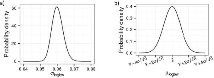
Posterior distributions of parameters of log‐normal distribution for body weight of 1‐year‐old children. The left panel shows the probability density for σ_logbw,  the standard deviation of log bw. The panel on the right shows the conditional probability density for μ_logbw, the mean of log bw, given a value for the standard deviation σ_logbw

However, when using these distributions in the exposure assessment, it is convenient to take a Monte Carlo sample from the posterior distribution to represent the uncertainty about μ_logbw and σ_logbw. This can be done as follows:

• Sample the required number of values of τ_logbw from the gamma distribution with shape = (171−1)/2 = 85 and rate = 85 * 0.060² = 0.306.

• For each value of τ_logbw in the previous step, calculate the corresponding value for ${\mathrm{\sigma }}_{\mathrm{logbw}}=1/\sqrt{{\mathrm{\tau }}_{\mathrm{logbw}}}$

• For each value of σ_logbw, sample a single value of μ_logbw from the normal distribution with mean 1.037 and standard deviation ${\mathrm{\sigma }}_{\mathrm{logbw}}/\sqrt{171}.$

The result of taking such a Monte Carlo sample is shown in Figure B.10 with the original sample mean and standard deviation for log bw shown, respectively, as dashed grey vertical and horizontal lines. The dependence between the two parameters is just visible in Figure B.10 (the mean is more uncertain when the standard deviation is high) but is not strong because the number of data n_logbw is large. Note that this particular Monte Carlo sampling process can easily be carried out in any standard spreadsheet software, for example, Microsoft Excel or LibreOffice Calc. In general, however, Bayesian analyses are better implemented using specialist software.

Figure B.10.

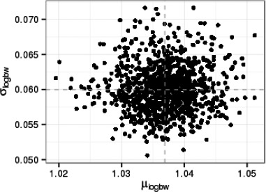
Monte Carlo sample of 1,000 values representing posterior uncertainty about σ_logbw and μ_logbw, given the data

Consumption (q)

For q, the statistical model is that: (i) q follows a gamma distribution with uncertain distribution parameters being the shape α_q and rate β_q; (ii) the data are a random sample from the distribution of q.

Again, no expert judgements were provided with which to inform the choice of prior distribution for the parameters. Instead, Jeffreys’ general prior is used (O'Hagan and Forster, 2004) which for this model has probability density function $\mathrm{p}({\mathrm{\alpha }}_{\mathrm{q}},{\mathrm{\beta }}_{\mathrm{q}})\infty (\sqrt{{\mathrm{\alpha }}_{\mathrm{q}}\mathrm{\psi }({\mathrm{\alpha }}_{\mathrm{q}})-1})/{\mathrm{\beta }}_{\mathrm{q}}.$

For this model and choice of prior distribution, there is no simple mathematical representation of the posterior distribution. However, it is still quite possible to obtain a Monte Carlo sample from the posterior distribution by various methods. The results below were obtained using the Metropolis random walk version of Markov Chain Monte Carlo (Gelman et al., 2015) to sample from the posterior distribution of α_q. Values for the rate parameter β_q were directly sampled from the conditional distribution of β_q given α_q,  for which there is a simple mathematical representation. Markov Chain Monte Carlo sampling of this kind is not easy to implement in a spreadsheet but takes only a few lines of code in software such as Matlab or R. This model is also easy to implement in software specialising in Bayesian inference, for example, WinBUGS, OpenBUGS or JAGS.

The results of taking a Monte Carlo sample representing uncertainty about the parameters are shown in Figure B.11a. This figure clearly shows the dependence between α_q and β_q. Figure B.11b shows the same uncertainty for the mean and coefficient of variation of the consumption distribution. The mean is α _q /β _q and the coefficient of variation is $1/\sqrt{{\mathrm{\alpha }}_{\mathrm{q}}}$. Values for these alternative parameters can be computed directly from the values of α_q and β_q in the Monte Carlo sample. In Figure B.11b, the mean and coefficient of variation of the data are shown, respectively, as dashed grey vertical and horizontal lines.

Figure B.11.

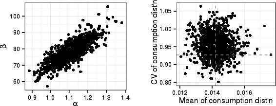
Monte Carlo sample representing posterior uncertainty about parameters for the gamma distribution describing variability of consumption. The left panel shows uncertainty about the shape and rate parameters. The panel on the right shows uncertainty about the mean (kg/day) and coefficient of variation of the consumption distribution

Strengths

1. Uncertainty about each parameter in a statistical model is quantified as a probability distribution for the possible values of the parameter. Therefore, the probability of different values of the parameter is quantified and this information can be taken into consideration by decision‐makers. Probability distributions for multiple uncertainties may be combined using the laws of probability.

2. Dependence of uncertainty for one or more parameters is expressed using a multivariate probability distribution. This is the most complete and theoretically based treatment of dependence that is possible with methods available today.

3. The statistical uncertainty due to having a limited amount of data is fully quantified.

4. Knowledge/information about parameter values from sources other than the data being modelled can be incorporated in the prior distribution by using expert knowledge elicitation (EKE).

5. The output of a Bayesian inference is usually most easily obtained as a Monte Carlo sample of possible parameter values and is ideally suited as an input to a 2D Monte Carlo analysis of uncertainty.

6. Bayesian inference can be used with all parametric statistical models.

Weaknesses and possible approaches to reduce them

1. Bayesian inference is an unfamiliar form of statistical inference in the EFSA community and may require the assistance of a statistician. By introducing this method in training courses for statistical staff at EFSA this weakness can effectively be remediated.

2. When it is required to do so, obtaining a prior distribution by EKE (see Section 11.3 and Annexes B.8 and B.9) can require significant time and resources.

3. When the prior distribution is not obtained by EKE, one must find another way to choose it and for most models there is not a consensus about the best choice. However, there is a substantial literature and one can also investigate the sensitivity of the posterior distribution to the choice of prior distribution. Moreover, the influence of the choice of prior on the posterior distribution diminishes at larger sample sizes.

4. There is less software available than for other methods of statistical inference and there is less familiarity with the available software. Training in the use of software could be included in training on Bayesian inference.

5. As with other methodologies for statistical inference, an inappropriate choice of statistical model can undermine the resulting inferences. It is important to consider carefully the (sampling) process by which the data were obtained and to carry traditional statistical model validation activities such as investigation of goodness of fit and looking for influential data values.

6. The need to use Markov chain Monte Carlo for more complex models introduces a further technical difficulty and potential source of uncertainty: the need to ensure that the Markov chain has reached equilibrium.

Assessment against evaluation criteria

This method is assessed against the criteria in Table B.23. All entries in the ‘Time Needed’ column have been highlighted because the time required for Bayesian inference is highly dependent on the complexity of the model. Overall, the ease or difficulty of applying Bayesian methods is strongly context dependent.

Table B.23.

Assessment of Probability bound analysis (when applied well) against evaluation criteria

Criteria	Evidence of current acceptance	Expertise needed to conduct	Time needed	Theoretical basis	Degree/extent of subjectivity	Method of propagation	Treatment of uncertainty and variability	Meaning of output	Transparency and reproducibility	Ease of understanding for non‐specialist
Stronger characteristics	International guidelines or standard scientific method	No specialist knowledge required	Hours	Well established, coherent basis for all aspects	Judgement used only to choose method of analysis	Calculation based on appropriate theory	Different types of uncertainty & variability quantified separately	Range and probability of possible answers	All aspects of process and reasoning fully documented	All aspects fully understandable
	EU level guidelines or widespread in practice	Can be used with guidelines or literature	Days	Most but not all aspects supported by theory	Combination of data and expert judgement	Formal expert judgement	Uncertainty and variability quantified separately	Range and relative possibility of answers	Most aspects of process and reasoning well documented	Outputs and most of process understandable
	National guidelines, or well established in practice or literature	Training course needed	Weeks	Some aspects supported by theory	Expert judgement on defined quantitative scales	Informal expert judgement	Uncertainty and variability distinguished qualitatively	Range of answers but no weighting	Process well documented but limited explanation of reasoning	Outputs and principles of process understandable
	Some publications and/or regulatory practice	Substantial expertise or experience needed	A few months	Limited theoretical basis	Expert judgement on defined ordinal scales	Calculation or matrices without theoretical basis		Quantitative measure of degree of uncertainty	Limited explanation of process and/or basis for conclusions	Outputs understandable but not process
Weaker characteristics	Newly developed	Professional statistician needed	Many months	Pragmatic approach without theoretical basis	Verbal description, no defined scale	No propagation	No distinction between variability and uncertainty	Ordinal scale or narrative description for degree of uncertainty	No explanation of process or basis for conclusions	Process and outputs only understandable for specialists

Conclusions

1. The method is suitable for application across EFSA, subject only to availability of the necessary statistical expertise.

2. It can be used for quantification of parameter uncertainty in all parametric statistical models.

3. For all except the simplest models, incorporating expert judgements in prior distributions is likely to require the development of further guidance on EKE.

References

Berry DA, 1995. Statistics: a Bayesian Perspective. Brooks/Cole.

EFSA PLH, PPR Panels, (Panel on Plant Health, Panel on Plant Protection Products and their Residues), 2006. Opinion of the Scientific Panel on Plant health, Plant protection products and their Residues on a request from EFSA related to the assessment of the acute and chronic risk to aquatic organisms with regard to the possibility of lowering the uncertainty factor if additional species were tested. The EFSA Journal (2005) 301, 1‐45.

EFSA (European Food Safety Authority), 2009. Meta‐analysis of Dose‐Effect Relationship of Cadmium for Benchmark Dose Evaluation. EFSA Scientific Report 254, 1‐62 http://www.efsa.europa.eu/sites/default/files/scientific_output/files/main_documents/254r.pdf

EFSA PPR Panel (EFSA Panel on Plant Protection Products and their Residues), 2012. Guidance on the Use of Probabilistic Methodology for Modelling Dietary Exposure to Pesticide Residues. EFSA Journal 2012;10(10):2839, 95 pp. https://doi.org/10.2903/j.efsa.2012.2839

EFSA PPR Panel (EFSA Panel on Plant Protection Products and their Residues), 2015. Scientific Opinion addressing the state of the science on risk assessment of plant protection products for non‐target arthropods. EFSA Journal 2015;13(2):3996, 212 pp. https://doi.org/10.2903/j.efsa.2015.3996

Gelman A, Carlin JB, Stern HS, Dunson DB, Vehtari A and Rubin DB, 2013. Bayesian Data Analysis, 3rd ed. Chapman & Hall/CRC.

Hald T, Pires SM and de Knegt L, 2012. Development of a Salmonella source attribution model for evaluating targets in the turkey meat production. EFSA Supporting Publications 2012:EN‐259.

Kruschke JK, 2010. Doing Bayesian Data Analysis: A Tutorial with R and BUGS. Academic Press.

O'Hagan A and Forster JJ, 2004. Kendall's advanced theory of statistics, volume 2B: Bayesian inference (Vol. 2). Arnold.

Teunis PFN and Havelaar AH, 2000. The beta poisson dose‐response model is not a single‐hit model. Risk Analysis 20(3): 513‐520.

Teunis PF, Ogden ID and Strachan NJ. Hierarchical dose response of E. coli O157:H7 from human outbreaks incorporating heterogeneity in exposure. Epidemiol Infect. 2008;136:761‐70.

Table B.22.

Assessment of Bayesian inference (when applied well) against evaluation criteria

Criteria	Evidence of current acceptance	Expertise needed to conduct	Time needed	Theoretical basis	Degree/extent of subjectivity	Method of propagation	Treatment of uncertainty and variability	Meaning of output	Transparency and reproducibility	Ease of understanding for non‐specialist
Stronger characteristics	International guidelines or standard scientific method	No specialist knowledge required	Hours	Well established, coherent basis for all aspects	Judgement used only to choose method of analysis	Calculation based on appropriate theory	Different types of uncertainty & variability quantified separately	Range and probability of possible answers	All aspects of process and reasoning fully documented	All aspects fully understandable
	EU level guidelines or widespread in practice	Can be used with guidelines or literature	Days	Most but not all aspects supported by theory	Combination of data and expert judgement	Formal expert judgement	Uncertainty and variability quantified separately	Range and relative possibility of answers	Most aspects of process and reasoning well documented	Outputs and most of process understandable
	National guidelines, or well established in practice or literature	Training course needed	Weeks	Some aspects supported by theory	Expert judgement on defined quantitative scales	Informal expert judgement	Uncertainty and variability distinguished qualitatively	Range of answers but no weighting	Process well documented but limited explanation of reasoning	Outputs and principles of process understandable
	Some publications and/or regulatory practice	Substantial expertise or experience needed	A few months	Limited theoretical basis	Expert judgement on defined ordinal scales	Calculation or matrices without theoretical basis		Quantitative measure of degree of uncertainty	Limited explanation of process and/or basis for conclusions	Outputs understandable but not process
Weaker characteristics	Newly developed	Professional statistician needed	Many months	Pragmatic approach without theoretical basis	Verbal description, no defined scale	No propagation	No distinction between variability and uncertainty	Ordinal scale or narrative description for degree of uncertainty	No explanation of process or basis for conclusions	Process and outputs only understandable for specialists

B.13. Probability bounds analysis

Purpose, origin and principal features

Probability bounds analysis provides a way of computing a probability bound relating to a combination of uncertainties based on probability bounds relating to individual uncertainties. This allows the use of probability to quantify uncertainty while at the same time allowing assessors to specify probability bounds rather than having to specify full probability distributions. A probability bound is an approximate probability for a specified range of possible values for a non‐variable quantity (parameter). The simplest useful form of probability bound is to specify an upper or lower limit on the probability that a parameter exceeds some specified level. Starting from probability bounds for individual inputs to a calculation (or a deterministic model), probability bounds analysis applies the laws of probability to deduce a probability bound for the output of the calculation, thereby quantifying combined uncertainty.

There is a long history in the theory of probability concerning methods for this kind of problem. It first appears in Boole (1854) and the simple methods presented here are based on Frechet (1935, 1951). A modern account of more complex approaches in the context of risk assessment is given by Tucker and Ferson (2003).

It is a generalisation of the interval analysis method (Annex B.7) but has the specific advantage that it incorporates some probability judgements and produces a partial expression of uncertainty using probability. The key advantage compared to Monte Carlo (Annex B.14) is that experts do not have to specify complete probability judgements; the least they must provide is an upper bound on the probability of exceeding (or falling below) some threshold for each source of uncertainty. A second advantage is that no assumptions are made about dependencies unless statements about dependence are specifically included in the calculation.

There are many possible ways in which it might be applied. The examples below show minimalist versions, based on the Frechet (1935, 1951) inequalities, for problems involving only uncertainty and problems involving both uncertainty and variability.

The two simplest versions are:

• Specify a probability bound for each of n inputs to a calculation: each probability bound consists of a range of values for the corresponding input and an approximate probability that the range contains the true value of the input. Probability bounds then provides a probability bound for the output value which would be obtained by using the true values of all the inputs in the calculation. The range for the output is obtained by applying interval analysis to the calculation using the input ranges specified in their probability bounds. The lower limit of the approximate probability for the output is then 1 − [(1 − p₁) + (1 − p₂) + … + (1 − p_n)] where p_i is the lower limit of the approximate probability attached to the range for the i th input. The upper limit of the approximate probability for the output may be in principle be less than 1 but this is difficult to determine without specialist expertise.

• For calculations which are monotonic increasing with respect to each input, i.e. increasing any single input always increases the output, a simple calculation yields a probability bound for the output. For each input, a probability bound of the following form must be specified: a value of interest for the input, together with an upper limit on the probability that the true value of the input exceeds the value specified. Then probability bounds analysis determines an upper limit for the probability that the output value corresponding to the true values of the inputs exceeds the output value corresponding to the values of interest specified for the inputs. The upper limit for the probability is obtained by summing the upper limits for the probabilities in the probability bounds specified for the inputs.

The first version is completely general and in fact the second version can be deduced straightforwardly from the first version. The second version is somewhat more generally applicable than it might appear. If a calculation is monotonic increasing with respect to some inputs and monotonic decreasing with respect to others, each input in the latter group can always be reparameterised so that the calculation becomes monotonic increasing with respect to all inputs; replace an input by its negation or a positive input by its reciprocal as in the example below.

By applying the probability bounds calculation twice, it is possible to obtain a probability bound for a percentile of the variable output of a monotonic calculation which has variable inputs. For details, see the example below.

Applicability in areas relevant for EFSA

Potentially applicable to all areas of EFSA's work but most obviously advantageous for assessments (or parts of assessments) for which probabilistic methods are considered to be too challenging.

Probability bounds analysis was used by EFSA (2017). Examples of use outside EFSA in risk assessment include Dixon (2007) and Regan et al. (2002).

Potential contribution to major elements of uncertainty analysis

Elements in uncertainty analysis	Potential contribution of this approach
Identifying uncertainties	Not applicable
Characterising uncertainties	Not applicable (required as input)
Combining uncertainties	Yes. However, simple versions do not involve quantification of dependencies but do allow for their possible existence in computing the bound on the combined impact
Prioritising uncertainties	Not applicable

Melamine example

In normal practice, the probability bounds on inputs required for probability bounds analysis would be obtained in most cases by expert knowledge elicitation (Sections B.8 and B.9). However, for the purpose of illustrating calculations based on probability bounds in the examples which follow, values specified for parameters, and bounds on probabilities of exceeding those values, were deduced from probability distributions used for Monte Carlo analyses (Annex B.14).

The melamine example (details in Annex C) has two versions: a worst‐case assessment and an assessment of uncertainty about variability. Both are considered below but require different approaches as only the second version directly involves variability.

Worst‐case exposure

The focus of this example is to make a partial probability statement about worst‐case exposure for children aged 1 up to 2 years, based on partial probability statements about individual parameters.

When increased, each of the following parameters increases the worst‐case exposure: c_max, w_max, q_max. When decreased, bw_min increases the worst‐case exposure and so increasing 1/bw_min increases the worst‐case exposure.

The following table shows a partial probability statement for each of the input parameters. The statements were derived from distributions used in Sections B.8 and B.9 but it is likely that expert knowledge elicitation would be used in many cases in real assessments.

Parameter	Specified value	Probability parameter exceeds specified value
cmax	3,750 mg/kg	≤ 3.5%
wmax	0.295	≤ 2%
qmax	0.095 kg	≤ 2.5%
1/bwmin	1/(5.6 kg)	≤ 2%

Note that the judgement for 1/bw_min was actually arrived by considering the probability that bw_min ≤ 5.6 kg.

The value being considered for e_max can then simply be calculated from the specified values for individual parameters which increase exposure: 3750 * 0.295 * 0.095/5.6 = 18.8

Based on the judgements in the preceding table, the laws of probability then imply that the probability that e_max exceeds 18.8 is less than (3.5 + 2 + 2.5 + 2)% = 10%. This is the simplest form of probability bounds analysis. No simulations are required.

As indicated earlier, the values specified for parameters and bounds on probabilities of exceeding those were obtained for illustrative purposes from the distributions used to represent in Sections B.8 and B.9. If the method were being applied using expert judgements about the parameters, we would be likely to end up with simpler probability values such as <=10%, <=5% or <=1% and the values specified for parameters would also be different having been specified directly by the experts. The method of computation would remain the same.

Uncertainty about variability of exposure

When variability is involved, the simplest approach to applying probability bounds analysis is to decide which percentile of the output variable will be of interest. The probability bounds method can then be applied twice in order to make an assessment of uncertainty about variability: once to variability and then a second time to uncertainty about particular percentiles.

For illustrative purposes, assessment will be made of uncertainty about the 95th percentile of exposure: e₉₅. In order to apply probability bounds analysis, for each input parameter a percentile needs to be chosen on which to focus. For illustrative purposes, it was decided to focus on the 98th percentile of variability of concentration, denoted c₉₈, and the 99th percentile of variability of each of the other input parameters which increase the exposure when increased: w₉₉, q₉₉ and (1/bw)₉₉. Note that (1/bw)₉₉ = bw₀₁.

Applying probability analysis first to variability, the mathematics of probability implies that ${\mathrm{e}}_{95}\ge {\mathrm{c}}_{98}\times {\mathrm{w}}_{99}\times {(1/\mathrm{bw})}_{99}={\mathrm{c}}_{98}\times {\mathrm{w}}_{99}\times {\mathrm{q}}_{99}/{\mathrm{bw}}_{01}$

where 95% is obtained as

$$95\%=100\%-[(100\%-98\%)+(100\%-99\%)+(100\%-99\%)+(100\%-99\%)]$$

The following table shows a partial probability statement of uncertainty about the chosen percentile for each of the input variables. As before, the statements were derived from distributions used in Sections B.8 and B.9 but it is likely that expert knowledge elicitation would be used in many cases in real assessments.

Parameter	Specified value	Probability parameter exceeds value specified
c98	4,400 mg/kg	≤ 2.5%
w99	0.295	≤ 2.5%
q99	0.075 kg	≤ 2.5%
(1/bw)99	1/(7 kg)	≤ 2.5%

Computing exposure using the values specified for the input parameters s leads to the following value to be considered for exposure: 4400 * 0.295 * 0.075/7 = 13.9. From this, by the same calculation as for worst‐case example, the laws of probability imply that the probability that c₉₈ × w₉₉ × q₉₉/bw₀₁ exceeds 13.9 is less than 2.5% + 2.5% + 2.5% + 2.5% = 10%.

Since e₉₅ ≥ c₉₈ × w₉₉ × q₉₉/bw₀₁, the probability that e₉₅ exceeds 13.9 is also less than 10%.

Various choices were made here:

• The choice of percentiles could have been made differently. It was assumed for illustrative purposes that the 95th percentile of exposure is of interest, although other percentiles could equally be considered. Given the focus on the 95th percentile, percentiles for the individual components were chosen so that the total variability not covered by them was less than or equal to 5%. Because there is reason to believe that the greatest source of variability is concentration, a lower percentile was chosen for concentration than for the other three parameters.

• Values specified for the percentiles of input parameters and probabilities of exceeding those values were obtained from the distributions used for the 2D Monte Carlo example in Sections B.8 and B.9. The total limit of the exceedance probability was chosen to be 10% and this was divided equally between the four parameters to illustrate the calculation. Any other division would have been valid and would have led to different values for the parameters.

• If expert knowledge elicitation were used instead to make a partial probability statement about each of the four percentiles, it is likely that simpler probability values such as ≤ 10%, ≤ 5% or ≤ 1% would have resulted, and the values specified for the percentiles would therefore also be different having been specified directly by the experts. The method of computation would remain the same.

Strengths

1. Simplest version provides an easily calculated bound on the probability that a calculated parameter exceeds a specified value. The method applies when a partial probability statement has been made about each input parameter and the calculation is monotonic with respect to each input.

2. Requires only probability bounds for inputs from experts. This greatly reduces the burden of elicitation compared to fully probabilistic methods.

3. Simple version makes no assumption about dependence between components of either uncertainty or variability.

4. More complex versions, based on the general theory of imprecise probability (Section 11.5.1) can in principle exploit more detailed probability judgements and/or statements about dependence of judgements.

Weaknesses and possible approaches to reduce them

1. For the simplest version, the calculated upper limit for the probability will be larger, and may be much larger, than would be obtained by a more refined probabilistic assessment. Nevertheless, it may sometimes be sufficient for decision‐making, and can indicate whether a more refined probabilistic assessment is needed.

2. Provides only a limited quantification of uncertainty about the calculated value. Nevertheless, that may sometimes be sufficient for decision‐making,

3. More complex versions involve more complex calculations and it is likely that professional mathematical/statistical advice would be needed.

Assessment against evaluation criteria

This method is assessed against the criteria in Table B.23. In evaluating time needed, only the simple form of probability bounds analysis was considered, as used in the two examples for melamine. Time needed to conduct EKE is not included.

Conclusions

1. This is potentially an important tool for EFSA as it provides a way to incorporate probabilistic judgements without requiring the specification of full probability distributions and without making assumptions about dependence. In so doing, it provides a bridge between interval analysis and Monte Carlo. It allows the consideration of less extreme cases than interval analysis and involves less work than full EKE for distributions followed by Monte Carlo.

2. Judgements and concept are rather similar to what EFSA experts do already when using assessment factors and conservative assumptions. Probability bounds analysis provides a transparent and mathematically rigorous calculation which results in an unambiguous quantitative probability statement for the output.

References

Boole G, 1854. An Investigation of the Laws of Thought on which are Founded the Mathematical Theories of Logic and Probabilities. Walton and Maberley.

Dixon WJ, 2007. The use of Probability Bounds Analysis for Characterising and Propagating Uncertainty in Species Sensitivity Distributions. Technical Report Series No. 163, Arthur Rylah Institute for Environmental Research, Department of Sustainability and Environment. Heidelberg, Victoria, Australia.

EFSA, 2017, Pilot study on uncertainty analysis in EFSA Reasoned Opinions on the modification of pesticide maximum residue levels. The EFSA Journal 15(7):4906. 52 pp.

Fréchet M, 1935. Généralisations du théorème des probabilités totales. Fundamenta Mathematica 25: 379–387.

Fréchet M, 1951. Sur les tableaux de corrélation dont les marges sont données. Annales de l'Université de Lyon. Section A: Sciences mathématiques et astronomie 9: 53–77.

Regan HM, Hope BK and Ferson S, 2002. Analysis and portrayal of uncertainty in a food web exposure model. Human and Ecological Risk Assessment 8: 1757–1777.

Tucker WT and Ferson S, 2003. Probability bounds analysis in environmental risk assessment. Applied Biomathematics, Setauket, New York. http://www.ramas.com/pbawhite.pdf

B.14. Monte Carlo simulation for uncertainty analysis (1D‐MC and 2D‐MC)

Purpose, origin and principal features

In the context of analysing uncertainty, Monte Carlo (MC) is primarily a computational tool for (i) calculations with probability distributions representing uncertainty and/or variability and (ii) those methods of sensitivity analysis (Annex B.17) which require sampling random values for parameters. In the case of (i), it provides a means to compute the combined effect of several sources of uncertainty, each expressed as a probability distribution, providing a probability distribution representing uncertainty about an assessment output. MC software often also provides modelling tools.

Monte Carlo simulation was developed in the 1940s, primarily by Stanislav Ulam in collaboration with Nicholas Metropolis and John von Neumann in the context of the Manhattan project to develop atomic bombs, and first published in 1949 (Ferson, 1996). Currently, the method is widely applied in science, finance, engineering, economics, decision analysis and other fields where random processes need to be evaluated. Many papers have been written about the history of MC simulation, the reader is referred to Bier and Lin (2013) and Burmaster and Anderson (1994).

In MC simulation for a quantitative model, uncertain parameters are represented by probability distributions expressing the uncertainty. Those probability distributions are the ‘inputs’ to the MC calculation. The model is recalculated many times, each time sampling a random value for each parameter from its distribution, to produce numerous scenarios or iterations. Each set of model results or ‘outputs’ from a single iteration represents a scenario that could occur. The joint distribution of outputs, across all the iterations, is a representation of the uncertainty in the outputs due to the uncertainty about the model parameters. Where the model also includes variable components, multiple values also need to be sampled for variables in each iteration of sampling values for uncertain parameters (the so‐called 2D Monte Carlo approach).

Risk assessment models may include variables that are correlated in some way. For example, the food consumption of a child will typically be less than that of an adult. Therefore, food consumption estimates are correlated with age and body weight. A cardinal rule to constructing a valid MC simulation is that ‘Each iteration of a risk analysis model must be a scenario that can physically occur’ (Vose, 2008, p. 63). There can also be dependence between uncertainties about parameters (see Section 5.4). If samples are drawn independently for two or more parameters or variables in an MC simulation, when in fact there should be dependence, this may result in selecting combinations that are not plausible. Ferson (1996) argues that the risk to exceed a particular threshold concentration depends strongly on the presence or absence of dependencies between model parameters and/or variables. Depending on whether correlations are positive or negative and the structure of the model, the exceedance risk may be underestimated or overestimated. A simple approach to addressing dependence between variables is to stratify the population into subgroups within which the inputs can be assumed not to be strongly correlated, but this may result in ad hoc solutions and tedious calculations. Different software packages offer different approaches to including correlations such as by specifying a correlation coefficient. However, even then only a small space of possible dependencies between the two variables may be sampled (US EPA, 1997). More advanced approaches include the use of copulas to specify the joint probability distribution of model inputs.

For assessments in which variability is not considered directly, for example, worst‐case assessments, MC can be used with all input distributions being representations of uncertainty. The MC output distribution will then also be a representation of uncertainty. However, for assessments involving variability and uncertainty about variability (see Section 5.3), it is important to differentiate between variable and uncertain factors when building MC simulations, in order to allow a more informative interpretation of the output distributions. Two‐dimensional Monte Carlo (2D‐MC) simulation was proposed by Frey (1992) as a way to construct MC simulations taking this separation into account. First, model inputs are classified to be either variable or uncertain. Uncertainty about variability can then be represented using a nested approach in which the distribution parameters, of probability distributions representing variability, are themselves assigned probability distributions representing uncertainty. For example, a dose–response model may be fitted to a data set involving a limited number of individuals, and the uncertainty of the fitted dose–response model might be represented by a sample from the joint distribution representing uncertainty about the dose–response parameters. The MC simulation is then constructed in two loops. In each iteration of the outer loop, a value is sampled for each uncertain model parameter, including distribution parameters. The inner loop samples a value for each variable component of the model and is evaluated as a 1D‐MC simulation, using the values sampled for distribution parameters in the outer loop to determine the probability distribution to use for each variable. This process will generate one possible realisation of all output values. The simulation is then repeated numerous times, usually repeating the inner loop many times per outer loop iteration. The outer loop iterations provide a sample of values for all uncertain parameters. For each outer loop iteration, the inner loop iterations provide a sample of values for variable components. In combination, they generate numerous possible realisations of distributions representing variability of outputs.

The results of a 2D‐MC simulation can be shown graphically as ‘spaghetti plots’, in which probability density functions (PDFs) or cumulative density functions (CDFs) of all simulated distributions of variability of inputs or outputs are plotted together. The spread in these distributions demonstrates the impact of uncertainty on the model output. Other commonly used graphics are probability bands (e.g. the median CDF and surrounding uncertainty intervals, see melamine example) or a combination of line‐ and box‐plots.

Software for MC simulation is commercially available as add‐ins to Excel such as @RISK, Crystal Ball and ModelRisk; and dedicated software such as Analytica. MC calculations can also be done in statistical software such as R, especially the distrfit and mc2d packages which support 2D‐MC (Pouillot and Delignette‐Muller, 2010), or SAS or mathematical software such as Mathematica or Matlab.

Applicability in areas relevant for EFSA

MC simulations are used in many domains of risk assessment including food safety. In EFSA, they are widely used in the area of microbial risk assessment and there is an EFSA guidance document on their application to pesticide exposure assessment, which includes use of 2D‐MC (EFSA, 2012).

Specific software applications are available to support MC simulations in different domains relevant for EFSA. These include FDA‐iRISK, sQMRA and MicroHibro for microbial risk assessment (reviewed in EFSA, 2015a,b,c), MCRA and Creme for human dietary exposure to chemicals, and Webfram for some aspects of environmental risk of pesticides.

The BIOHAZ Panel has commissioned several outsourced projects to develop complex models including Salmonella in pork (Hill et al., 2011) and BSE prions in bovine intestines and mesentery (EFSA, 2014a,b). The importance of 2D simulation was underlined, for example, by Nauta (2011) who demonstrated that a simple model for the growth of Bacillus cereus in pasteurised milk without separation of uncertainty and variability may predict the (average) risk to a random individual in an exposed population. By separating variability and uncertainty, the risk of an outbreak can also be identified, as cases do not occur randomly in the population but are clustered because growth will be particularly high in certain containers of milk.

Pesticide intake rate for certain bee species was modelled by EFSA's PRAS Unit using MC simulation techniques. The 90th percentile of the residue intake rate and its 95% confidence interval were derived from the empirical joint distribution of the feed consumption and residue level in pollen and nectar.

Trudel et al. (2011) developed a 2D‐MC simulation to investigate whether enhancing the data sets for chemical concentrations would reduce uncertainty in the exposure assessment for the Irish population to polybrominated diphenyl ethers and concluded that ‘by considering uncertainty and variability in concentration data, margins of safety (MOS) were derived that were lower by a factor of 2 compared to MOS based on dose estimates that only consider variability’. Based on the simulation results, they also suggested that ‘the datasets contained little uncertainty, and additional measurements would not significantly improve the quality of the dose estimates’.

MC simulations are used by FAO/WHO committees supporting the work of the Codex Alimentarius Commission (JECFA, JMPR, JEMRA), as well as by national risk assessment agencies (RIVM, BfR, ANSES, and others). They are commonly used for exposure assessment in chemical risk assessment (US FDA), but not yet common in toxicology. In the USA, an interagency guideline document (USDA/FDIS and US EPA, 2012) for microbial risk assessment features MC simulations prominently for exposure assessment and risk characterisation.

There are many guidelines and books that provide detailed instructions on how to set up MC simulations. Burmaster and Anderson (1994), Cullen and Frey (1999) and Vose (2008) all have an emphasis on the risk assessment domain. USEPA (1997) have published Guiding Principles on the use of MC analysis, which are very relevant to applications in EFSA.

Potential contribution to major elements of uncertainty analysis

Elements in uncertainty analysis	Potential contribution of this approach
Identifying uncertainties	Not applicable
Characterising uncertainties	Not applicable (required as input)
Combining uncertainties	Yes, rigorous quantification of the impact of quantified input uncertainties on the output uncertainty, subject to model assumptions
Prioritising uncertainties	Yes, rigorous quantification of the contribution of input uncertainties to combined uncertainty

Melamine example

Two examples are presented of the use of MC for assessment of uncertainty. The first illustrates how ordinary (1D) MC may be used, for assessments where variability is not modelled, to calculate uncertainty about assessment outputs based on probability distributions representing uncertainty about input parameters. It assesses uncertainty about the worst‐case exposure for children aged from 1 up to 2 years. The second example illustrates how 2D‐MC may be used as a tool in assessing uncertainty about variability in assessments where that is an issue. It considers uncertainty about variability of exposure for those children in the same age group who consume contaminated chocolate from China.

Details of the models used may be found in Annex C together with details and some analysis of data which were the basis for some distributions used in the 2D example.

Worst‐case assessment

For simplicity, this example focuses only on selected uncertainties affecting the estimate of worst‐case exposure for children aged from 1 up to 2 years. In particular, any uncertainties affecting the TDI are not considered. A combined characterisation of uncertainty would need to include these and additional uncertainties affecting exposure. Distributions used to represent uncertainty about parameters were not obtained by careful elicitation of judgements from relevant experts. Rather, they are provided so that the MC calculations and output can be illustrated. Consequently, only a limited amount of reasoning is provided as it is likely that a real assessment would make different choices.

The worst‐case exposure is obtained by

$${\mathrm{e}}_{\max }=\frac{{\mathrm{c}}_{\max }\times {\mathrm{w}}_{\max }\times {\mathrm{q}}_{\max }}{{\mathrm{bw}}_{\min }}$$

and the worst‐case risk ratio is then r_max = e_max/TDI.

To build a MC simulation, a distribution must be provided for each uncertain input parameter. The distributions used for this example are shown in Figure B.13. For each parameter, the distribution is over the range of values used for the parameter in the final table of the interval analysis (Annex B.7) example.

Figure B.13.

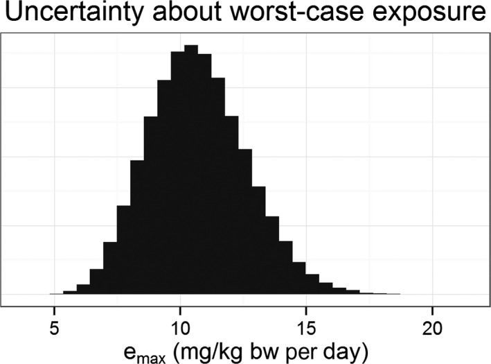
Uncertainty, calculated by MC, about worst‐case exposure for children aged from 1 up to 2 years

The triangular distribution with 5.5 and 6.5 as endpoints and peak at 6 was selected to represent uncertainty about bw_min.

The triangular distribution with 0.05 and 0.10 as the endpoints and with peak at 0.075 was selected to represent uncertainty about q_max.

For uncertainty about w_max, the distribution obtained in the hypothetical example of expert knowledge elicitation example (Sections B.8 and B.9) was used.

For uncertainty about c_max,  a PERT distribution (Vose, 2008) was selected: the PERT distribution is a beta distribution rescaled to have a specified minimum and maximum. The beta distribution with parameters 3.224 and 16.776 was rescaled to the range from 2,563 to 6,100 mg/kg and the mode of the resulting distribution is at 3,100 mg/kg was selected. Like the triangular distribution family, the beta PERT distribution family only assigns non‐zero probability to a finite range of values. However, it has the additional possibility for the probability density function to descend more quickly to zero near the endpoints. This was felt to be particularly desirable for the upper endpoint since there would actually be no milk in the dried matter at that endpoint and so such values would be very unlikely.

Figure B.12.

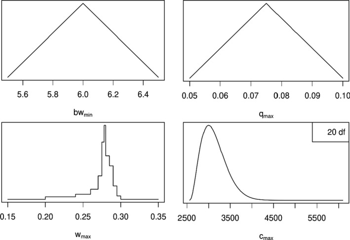
Distributions used to represent uncertainty about input parameters in worst‐case exposure assessment for children aged from 1 up to 2 years

The MC simulation was built in R version 3.1.2 (R Core team, 2014), using the package mc2d (Pouillot and Delignette‐Muller, 2010).

The output of the MC simulation is a distribution, shown in Figure B.13, representing uncertainty about e_max. The output is calculated from the distributions selected to represent uncertainty about input parameters. Table B.24 summarises the output and compares it to the TDI. The benefit of carrying out a MC analysis is that there is a full distribution representing uncertainty. This provides greater detail than other methods.

Table B.24.

Uncertainty, calculated by MC, about the worst‐case exposure and ratio to TDI for children aged from 1 up to 2 years

		Worst–case exposure (emax)	Risk ratio (r) (emax/TDI)
Summary of uncertainty distribution	Median	10.6	21.2
	Mean	10.7	21.4
	2.5%‐ile	7.7	14.3
	97.5%‐ile	14.8	29.5

Uncertainty about variability of exposure

For simplicity, this example focuses only on selected uncertainties affecting the estimate of worst‐case exposure for children aged from 1 up to 2 years who consume contaminated chocolate from China. In particular, no consideration is given to (i) uncertainties affecting the TDI; (ii) uncertainties about the relevance of data used; (iii) uncertainties about distribution family choices. A combined characterisation of uncertainty would need to include these and any other additional uncertainties. Distributions used to represent uncertainty about parameters are not considered to be the best possible choices. Rather, they are provided so that the MC calculations and output can be illustrated. Consequently, only a limited amount of reasoning is provided as it is likely that a real assessment would make different choices.

The assessment model (further details in Annex C), in which all inputs are variable, is

$$\mathrm{e}=\frac{\mathrm{c}\times \mathrm{w}\times \mathrm{q}}{\mathrm{bw}}$$

To carry out a 2D‐MC simulation for this model, it is necessary first, for each input, to choose a suitable distribution to model variability. The approach taken here is to choose a parametric distribution family for each input. It would also be possible to proceed non‐parametrically if suitable data were to be available for a variable; in that situation, uncertainty about variability might be addressed by using the bootstrap (Annex B.11).

The distribution family choices are shown in the second column of Table B.25. For body weight (bw) and consumption (q), they were based on analysis of data described in Annex C. For concentration (c) and weight‐fraction (w), they are purely illustrative. The restrictions applied to the range of variability of bw, q and c derive from the worst‐case limits used in the interval analysis example (Annex B.7).

Table B.25.

Summary of distribution families used to model variability of input parameters and of distributions used to represent uncertainty about variability distribution parameters

Parameter	Model for variability (distribution family)	Uncertainty about variability distribution parameters
Body weight (bw, kg)	Log‐normal (restricted to a minimum of 5.5 kg)	Posterior distribution from Bayesian inference (Annex B.12) applied to data described in Annex C. Figure B.10 shows a sample from the posterior distribution
Consumption (q, kg/day)	Gamma (restricted to a maximum of 0.1 kg/day)	Posterior distribution from Bayesian inference (Annex B.12) applied to data described in Annex C. Figure B.11 shows a sample from the posterior distribution
Concentration(c, mg/kg)	Log‐normal (restricted to a maximum of 6,100 mg/kg)	Median fixed at 29 mg/kg. Beta(22,1) distribution used to represent uncertainty about percentile to which maximum data value 2,563 mg/kg corresponds
Weight‐fraction (w, ‐)	Uniform	Lower end of uniform distribution fixed at 0.14. Uncertainty about upper end represented by distribution for wmax used in the worst‐case example above

Having chosen distribution families to represent variability, the next step is to specify distributions representing uncertainty about distribution parameters and to decide how to sample from them. The choices made are summarised in the third column of Table B.25 and some further details follow.

1. The EFSA statement refers to data on concentrations in infant formula. Those data were not obtained by random sampling and only summaries are available. The median of those data was 29 mg/kg and the maximum value observed was 2,563 mg/kg. In the 2D‐MC simulation, the median of the log‐normal distribution for concentrations was taken to be 29 mg/kg. In reality, the median concentration is uncertain and so this choice introduces an additional uncertainty which is not addressed by the MC analysis. The percentile of the concentration distribution corresponding to the maximum data value of 2,563 mg/kg is considered to be uncertain. Treating the maximum data value as having arisen from a random sample of size 22, both Bayesian and non‐Bayesian arguments lead to a beta(22, 1) distribution for the percentile to which 2,563 corresponds. When implementing 2D‐MC, a value is sampled from the beta distribution in each iteration of the outer loop; from that value, it is possible to calculate the standard deviation for the underlying normal distribution which would place 2,563 at the specified percentile.

2. Sampling from the posterior distribution for the parameters of the log‐normal distribution for body weight was carried out by the MC method described in the example in Annex B.12.

3. Sampling from the posterior distribution for the parameters of the gamma distribution for consumption was carried out by Markov Chain MC as described in the example in Annex B.12.

4. Sampling from the distribution for w_max could be carried out several ways. The method used in producing the results shown below was to treat the distribution as a 12 component mixture of uniform distributions and to sample accordingly.

A by‐product of the 2D‐MC calculation is that the samples can be used to summarise the input variables in various ways. For each variable, Table B.26 summarises uncertainty about five variability statistics: mean, standard deviation and three percentiles of variability. Uncertainty is summarised by showing the median estimate, the mean estimate and upper and lower 2.5th and 97.5th percentiles of uncertainty for each variability statistic. The two percentiles of uncertainty together make up a 95% uncertainty interval. For example, if one is interested in the mean body weight of children aged 1 up to 2 years, the median estimate is 11.0 kg and the 95% uncertainty interval is (10.8, 11.2)kg.

Table B.26.

Summaries, based on 2D‐MC output, of uncertainty about variability for each of the assessment inputs

Variable	Uncertainty	Variability
		Mean	St. dev.	2.5%	50%	97.5%
c (mg/kg)	50%	225.2	617	0.262	27.8	2059
	2.5%	83.7	198	0.002	14.9	509
	97.5%	377.3	947	1.629	29.9	3791
w (‐)	50%	0.209	0.039	0.143	0.209	0.275
	2.5%	0.176	0.021	0.142	0.176	0.211
	97.5%	0.217	0.044	0.144	0.217	0.290
q (kg/day)	50%	0.014	0.013	0.00042	0.010	0.050
	2.5%	0.013	0.012	0.00031	0.0091	0.045
	97.5%	0.016	0.015	0.00069	0.0114	0.056
bw (kg)	50%	11.0	1.53	8.30	10.9	14.3
	2.5%	10.8	1.37	7.98	10.7	13.8
	97.5%	11.2	1.72	8.59	11.1	14.8

Turning to uncertainty about assessment outputs, the results of the 2D‐MC simulation are shown in Tables B.27 and B.28. Table B.27 shows summaries of uncertainty about four exposure variability statistics: the mean and three percentiles. For each variability statistic, the median estimate is shown along with two percentiles which together make up a 95% uncertainty interval. For example, for mean exposure, the median estimate is 0.0605 mg/kg bw per day and the 95% uncertainty interval ranges between 0.022 and 0.105 mg/kg bw per day. Table B.28 summarises uncertainty about the percentage of person‐days for which exposure exceeds the TDI of 0.5 mg/kg bw.

Table B.27.

Summaries of uncertainty, based on 2D‐MC output, of uncertainty about variability of exposure for children aged from 1 up to 2 years

Uncertainty	Variability
	Mean	2.5%‐ile	Median	97.5%‐ile
Median	0.0605	2.0e‐5	0.0045	0.527
2.5%‐ile	0.0224	3.7e‐7	0.0023	0.154
97.5%‐ile	0.1052	9.0e‐5	0.0054	1.037

Table B.28.

Uncertainty, based on 2D‐MC output, about the percentage of child‐days (1 year olds consuming contaminated chocolate from China) exceeding the TDI of 0.5 mg/kg per day

	Percentage of child‐days exceeding TDI
Median estimate	2.7%
95% uncertainty interval	(0.4, 5.5)%

The results can also be presented graphically as a series of cumulative distribution functions. Figures B.14 and B.15 show uncertainty about variability of the risk ratio r. In these figures, the spread of the curve along the y‐axis (the grey‐shaded areas) represents uncertainty about the fraction of child‐days where the risk ratio exceeds the value on the x‐axis. From these graphs, it is clear that, subject to the assumptions made in building the 2D‐MC simulation, there is major variability in the exposure to melamine, and hence in the risk ratio. The majority of 1 year old children consuming chocolate from China contaminated with melamine will be exposed to low levels but it is estimated that 2.7% (95% CI 0.4–5.5%) of those child‐days have melamine exposure above TDI.

Figure B.14.

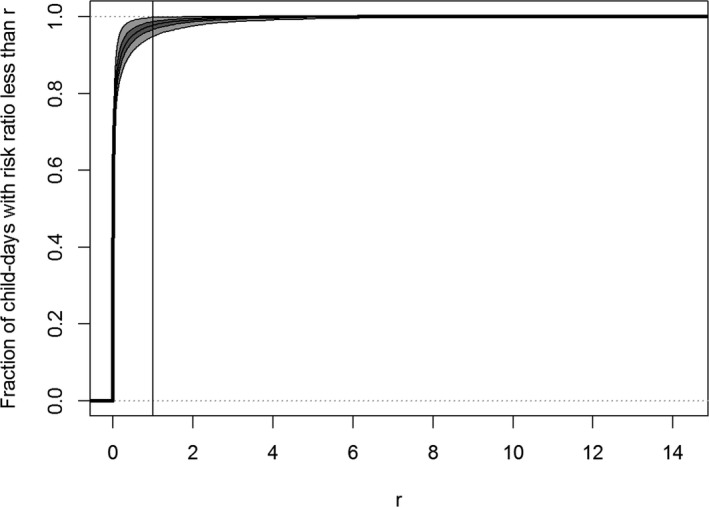
Plot of estimated cumulative distribution of ratio of exposure to the TDI for melamine, for 1‐year‐olds consuming contaminated chocolate from China. Uncertainty about the cumulative distribution is indicated: the light grey band corresponds to 95% uncertainty range, and dark grey band corresponds to 50% uncertainty range

Figure B.15.

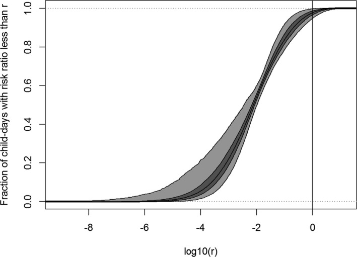
Plot, as in Figure B.14 but with logarithmic scale for r, of cumulative distribution of ratio of exposure to the TDI for melamine, for 1‐year‐olds consuming contaminated chocolate from China. Uncertainty about the cumulative distribution is indicated: the light grey band corresponds to 95% uncertainty range, and dark grey band corresponds to 50% uncertainty range

Strengths

1. Provides a fully quantitative method for propagating uncertainties, which is more reliable than semi‐quantitative or qualitative approaches or expert judgement.

2. Is a valid mathematical technique, subject to the validity of the model and inputs.

3. Can simulate complex models and changes to a model can be made quickly and results compared with previous models.

4. Level of mathematics required is quite basic, but complex mathematics can be included.

5. Two‐dimensional MC is capable of quantifying uncertainty about variability.

6. Model behaviour can be investigated relatively easily.

7. Time to results is reasonably short with modern computers.

8. Correlations and other dependencies can be addressed (but it can be difficult in some software, and is often not done).

Weaknesses and possible approaches to reduce them

1. If the input distributions are uncertain MC needs to be combined with sensitivity analysis (Annex B.17).

2. Obtaining appropriate data to define input distributions may be data‐intensive (but structured expert elicitation is an alternative).

3. MC requires estimates or assumptions for the statistical dependencies among the variables. Uncertainty affecting these may be substantial and, if not quantified within the model, must be taken into account when characterising combined uncertainty. Sensitivity analysis may help.

4. One‐dimensional MC does not distinguish between variability and uncertainty. Two‐dimensional MC addresses this.

The relationship between inputs and outputs is unidirectional. New data can only be used to update the probability distribution of one input factor but not the joint distribution of all input factors. However, this is possible using more advanced forms of Bayesian modelling and inference such as Bayesian graphical models.

Assessment against evaluation criteria

This method is assessed against the criteria in Table B.29.

Table B.29.

Assessment of 1D‐MC (grey) and 2D‐MC (dark grey, where different from 1D‐MC), when applied well against evaluation criteria

Criteria	Evidence of current acceptance	Expertise needed to conduct	Time needed	Theoretical basis	Degree/extent of subjectivity	Method of propagation	Treatment of uncertainty & variability	Meaning of output	Transparency and reproducibility	Ease of understanding for non‐specialist
Stronger characteristics	International guidelines available	No specialist knowledge required	Hours	Well established, coherent basis for all aspects	Fully data based	Calculation based on appropriate theory	Different types of uncertainty & variability quantified separately	Range and probability of possible answers	All aspects of process and reasoning fully documented	All aspects fully understandable
	EU level guidelines available	Can be used with guidelines or literature	Days	Most but not all aspects supported by theory	Combination of data and expert judgement	Formal expert judgement	Uncertainty and variability quantified separately	Range and relative possibility of answers	Most aspects of process and reasoning well documented	Outputs and most of process understandable
	National guidelines, or well established in practice or literature	Training course needed	Weeks	Some aspects supported by theory	Expert judgement on defined quantitative scales	Informal expert judgement	Uncertainty and variability distinguished qualitatively	Range of answers but no weighting	Process well documented but limited explanation of reasoning	Outputs and principles of process understandable
	Some publications and/or regulatory practice	Substantial expertise or experience needed	A few months	Limited theoretical basis	Expert judgement on defined ordinal scales	Calculation or matrices without theoretical basis		Quantitative measure of degree of uncertainty	Limited explanation of process and/or basis for conclusions	Outputs understandable but not process
Weaker characteristics	Newly developed	Professional statistician needed	Many months	Pragmatic approach without theoretical basis	Verbal description, no defined scale	No propagation	No distinction between variability and uncertainty	Ordinal scale or narrative description for degree of uncertainty	No explanation of process or basis for conclusions	Process and outputs only understandable for specialists

Conclusions

1. MC is the most practical way to carry fully probabilistic assessments of uncertainty and uncertainty about variability and is therefore a very important tool.

2. Application of MC is demanding because it requires full probability distributions. Two‐dimensional MC is particularly demanding because it requires modelling choices (distribution families) and quantification of uncertainty about distribution parameters using statistical inference from data and/or expert knowledge elicitation.

3. It is likely that MC will be used to quantify key uncertainties in some assessments, especially in assessments where variability is modelled, with other methods being used to address other uncertainties.

4. MC output can be used to make partial probability statements concerning selected parameters which can then be combined with other partial probability statements using probability bounds analysis.

References

Bier VM and Lin SW. On the treatment of uncertainty and variability in making decisions about risk. Risk Anal. 2013;33(10):1899–907.

Burmaster DE and Anderson PD, 1994. Principles of good practice for the use of Monte Carlo techniques in human health and ecological risk assessments. Risk Analysis. 1994;14(4):477–81.

Cullen AC, Frey HC, 1999. Probabilistic Techniques in Exposure Assessment: A Handbook for Dealing with Variability and Uncertainty in Models and Inputs. New York: Plenum Press; 1999.

EFSA Scientific Committee, 2012. Guidance on selected default values to be used by the EFSA Scientific Committee, Scientific Panels and Units in the absence of actual measured data. EFSA Journal 2012;10(3):2579.

EFSA (European Food Safety Authority), 2008. Statement of EFSA on risks for public health due to the presences of melamine in infant milk and other milk products in China. EFSA Journal 2008;807: 1–10.

EFSA PPR Panel (Panel on Plant Protection Products and their Residues.) Guidance on the Use of Probabilistic Methodology for Modelling Dietary Exposure to Pesticide Residues. EFSA Journal 2012;10(10):2839, 95 pp. https://doi.org/10.2903/j.efsa.2012.2839.

EFSA BIOHAZ Panel (EFSA Panel on Biological Hazards), 2014. Scientific Opinion on BSE risk in bovine intestines and mesentery. EFSA Journal 2014;12(2):3554, 98 pp. https://doi.org/10.2903/j.efsa.2014.3554

Ferson S. What Monte Carlo methods cannot do. Human and Ecological Risk Assessment. 1996;2:990–1007.

Frey, H.C., 1992. Quantitative analysis of uncertainty and variability in environmental policy making. Fellowship Program for Environmental Science and Engineering, American Association for the Advancement of Science, Washington, DC.

Hill A, Simons R, Ramnial V, Tennant J, Denman S, Cheney T, et al. Quantitative Microbiological Risk Assessment on Salmonella in slaughter and breeder pigs: final report. Parma, Italy: European Food Safety Authority, 2011 EN‐46. http://www.efsa.europa.eu/sites/default/files/scientific_output/files/main_documents/46e.pdf

Nauta MJ, 2000. Separation of uncertainty and variability in quantitative microbial risk assessment models. International Journal of Food Microbiology, 57(1), 9–18.

Pouillot R AND Delignette‐Muller ML, 2010. Evaluating variability and uncertainty separately in microbial quantitative risk assessment using two R packages. Int J Food Microbiol. 2010;142(3):330–340.

R Core Team, 2014. R: A language and environment for statistical computing. R Foundation for Statistical Computing, Vienna, Austria. URL http://www.R-project.org/

Trudel D, Tlustos C, von Goetz N, Scheringer M, Reichert P and Hungerbuhler K, 2011. Exposure of the Irish population to PBDEs in food: consideration of parameter uncertainty and variability for risk assessment. Food Addit Contam A. 2011;28(7):943–55.

US EPA, 1997. Guiding Principles for Monte Carlo Analysis. EPA/630/R‐97/001. US EPA Risk Assessment Forum.

USDA/FDIS and US EPA, 2012. U.S. Department of Agriculture/Food Safety and Inspection Service and U.S. Environmental Protection Agency. Microbial Risk Assessment Guideline: Pathogenic Organisms with Focus on Food and Water. FSIS Publication No. USDA/FSIS/2012‐001; EPA Publication No. EPA/100/J12/001.

Vose D. Risk analysis ‐ a quantitative guide. Third ed. Chichester, England: John Wiley & Sons; 2008.

B.15. Approximate probability calculations

B.15.1.

B.15.1.1.

Purpose, origin and principal features

The purpose of this method is to provide simple calculations to find an approximation to the probability distribution which represents the combination of a number of uncertain components. Two versions are provided: one suitable for situations where uncertain components are being added and the other for situations where components are being multiplied. Both versions are based on using normal distributions to approximate other distributions.

Like probability bounds analysis (Annex B.13) and Monte Carlo (Annex B.14), this method uses the mathematics of probability. The method is fully probabilistic but calculates an approximate distribution representing the combination of uncertain components whereas Monte Carlo computes the distribution correctly provided that the Monte Carlo sample size is large enough and probability bounds analysis does not compute the full distribution but provides only one or more partial probability statements.

The usefulness of normal distributions in many ways, including easy calculations for adding independent normal distributions, is a core part of the development of the theories of probability and statistics (for example, Rice, 2006). A calculation of the kind described here was proposed by Gaylor and Kodell (2000) for determining assessment factors in the context of risk assessment for humans exposed to non‐carcinogens. IPCS (2014) proposed using this kind of approximation to a more complex model to be used for hazard characterisation for chemicals.

Version A (adding m uncertain components):

$${\mathrm{U}}_{\mathrm{combined}}={\mathrm{U}}_1\pm {\mathrm{U}}_2\pm \dots +{\mathrm{U}}_{\mathrm{m}}$$

The probability distribution representing uncertainty about each individual component U_i is approximated by a normal distribution. In making the approximation for each individual component, a mean μ_i and standard deviation σ_i have to be chosen for each component. The approximate distribution representing uncertainty about the sum of the components U_combined is then also a normal distribution. The mean of that distribution is μ_combined = μ₁ + … + μ_m and the standard deviation is ${\mathrm{\sigma }}_{\mathrm{combined}}=\sqrt{{\mathrm{\sigma }}_1^2+\dots +{\mathrm{\sigma }}_{\mathrm{m}}^2}.$

Version B (multiplying m uncertain components):

$${\mathrm{U}}_{\mathrm{combined}}={\mathrm{U}}_1\times {\mathrm{U}}_2\times \dots \times {\mathrm{U}}_{\mathrm{m}}$$

The probability distribution representing uncertainty about each individual component U_i is approximated by a log‐normal distribution. The approximate distribution representing uncertainty about the product of the components is then also a log‐normal distribution. This is really version A applied to

$$\text{log}{\mathrm{U}}_{\mathrm{combined}}=\text{log}{\mathrm{U}}_1+\text{log}{\mathrm{U}}_2+\dots +\text{log}{\mathrm{U}}_{\mathrm{m}}$$

The distribution approximating each logU_i is normal and the mean μ_i and standard deviation σ_i have to be specified for each logU_i. These are then combined as in version A to obtain μ_combined and σ_combined which are the mean and standard deviation for logU_combined.

For both versions, a way has to be found to determine μ_i and σ_i for each component. In version A, if the mean and standard deviation of the distribution of U_i are known, these can be used. Alternatively, if any two percentiles are known, these can be used to determine μ_i and standard deviation σ_i by assuming that the approximating distribution should have the same percentiles. For version B, if the geometric mean and geometric standard deviation of U_i are known, the logarithms of these values are the mean and standard deviation of logU_i and can be used as μ_i and σ_i. Alternatively, if any two percentiles of U_i are known, their logarithms are the corresponding percentiles of logU_i and can then be used as in version A to determine μ_i and σ_i.

The method will be exact (no approximation) in two situations: when the original distribution for each U_i is normal in version A and when the original distribution for each U_i is log‐normal in version B. In all other situations, the distribution obtained for U_combined will be an approximation. There is no easy way to determine how accurate the approximation will be. The central limit theorem (for example, Rice, 2006) gives some grounds for expecting the approximation to improve as m gets larger, provided that the standard deviations σ₁, …, σ_m are similar.

The approximate distribution obtained for the combined uncertainty will generally depend on how the individual μ_i and σ_i are obtained. Using percentiles will generally give a different result to using means and standard deviations; using different percentiles will also usually give different results. It is not possible to say in general what would be the best percentiles to use.

It is in principle possible to include dependencies by specifying correlations between pairs of individual uncertainties in version A (between logU_i in version B). This requires a more complicated calculation based on the multivariate normal distribution to find the distribution of U_combined (logU_combined in version B). Details of how to work with the multivariate normal distribution may be found in, for example, Krzanowski (2000).

It is theoretically possible that there may be other versions of this kind of calculation but there are no others which are clearly useful now for EFSA assessments. It does not seem likely that it can easily be applied to situations involving uncertainty about variability.

Applicability in areas relevant for EFSA

In principle, the method is applicable to any area of EFSA's work. It is restricted to situations where the model or part of the model involves adding or multiplying, but not both adding and multiplying, independent uncertain components. In such situations, distributions representing individual uncertainties can be approximated using distributions from the relevant family. The latter are then combined to provide a distribution from the same family which approximately represents the combined uncertainty.

Gaylor and Kodell (2000) proposed using this approach to derive assessment factors to apply to animal data in the context of toxicity to humans of non‐carcinogenic chemicals. For the same context, IPCS (2014) developed a more sophisticated multiplicative model for determining a chemical specific assessment factor subject to assumptions about suitability of underlying databases. Full implementation of the IPCS (2014) model needs Monte Carlo calculations. The approach described in this appendix was applied by IPCS (2014) to their model and the resulting calculation was made available in the APROBA tool implemented in Excel.

Potential contribution to the main elements of uncertainty analysis

Elements in uncertainty analysis	Potential contribution of this approach
Identifying uncertainties	Not applicable
Characterising uncertainties	Not applicable (required as input)
Combining uncertainties	Yes. However, dependencies are not straightforward to address
Prioritising uncertainties	Not applicable

Melamine example

The focus of this example is to derive a probability distribution which approximately represents uncertainty about worst‐case exposure for children aged 1 up to 2 years. The exposure calculation involves only multiplication and division. It is therefore suitable for application of the approximate probability calculation method using log‐normal distributions to approximately represent individual uncertainties. The starting point is to determine a log‐normal distribution approximately representing uncertainty for each of ${\mathrm{c}}_{\max },{\mathrm{w}}_{\max },{\mathrm{q}}_{\max }$ and bw_min.

The most straightforward way to find a log‐normal distribution approximately representing uncertainty about a positive parameter is to specify two percentiles of uncertainty about the parameter and use those to determine the mean and standard deviation of the logarithm of each parameter. The following table shows the percentiles used in the example.

Parameter	Median	Tail percentile used	Tail percentile value	Logarithm (base 10) of median	Logarithm (base 10) of tail percentile
cmax (mg/kg)	3,093	96.5th %ile	3728	log10 3093 = 3.490	log10 3728 = 3.571
wmax (‐)	0.278	98th %ile	0.294	log10 0.278 = –0.556	log10 0.294 = –0.532
qmax (kg/day)	0.075	97.5th %ile	0.094	log10 0.075 = –1.125	log10 0.094 = –1.027
bwmin (kg)	6.00	2nd %ile	5.60	log10 6.00 = 0.778	log10 5.60 = 0.748

The next table shows how these values are used to obtain the mean and standard deviation for the logarithm of each parameter:

Parameter	Mean of log‐parameter	Tail percentile used	z‐value (percentile of standard normal)	SD of log‐parameter
cmax	3.490	96.5th	1.812	(3.571–3.490)/1.812 = 0.045
wmax	–0.556	98th	2.054	(−0.352–(−0.556))/2.054 = 0.012
qmax	–1.125	97.5th	1.960	(−1.027–(−1.125))/1.960 = 0.050
bwmin	0.778	2nd	–2.054	(0.748–0.778)/(−2.054) = 0.015

The mean of the approximate normal distribution for the logarithm of e_max is then obtained by adding the means for the logarithm of each of c_max, w_max, q_max and subtracting the mean for the logarithm of bw_min: 3.490 – 0.556 – 1.125 – 0.778 = 1.031.

The standard deviation of the approximate normal distribution for the logarithm of e_max is obtained by adding the squares of the standard deviations (for the logarithms of the parameters) and then taking the square‐root: $\sqrt{0.{045}^2+0.{012}^2+0.{050}^2+0.{015}^2}=0.070$.

From this distribution approximately representing uncertainty about the logarithm of e_max, we can then obtain an approximate value for any percentile of e_max or calculate an approximate probability for exceeding any specified value for e_max. For example, the median of uncertainty about log₁₀e_max is approximately 1.031 and so the median of uncertainty about e_max is approximately 10^1.031 = 10.74 mg/kg bw per day. The 90th percentile of uncertainty about log₁₀e_max is 1.031 + 1.282 × 0.070 = 1.121 and so the 90th percentile of uncertainty about e_max is approximately 10^1.121 = 13.24 mg/kg bw per day.

The medians and percentiles used above were obtained from the distributions used to represent uncertainty about each of c_max, w_max, q_max, and bw_min in the 1D Monte Carlo example in Annex B.14. The following figure shows each of those distributions as a probability density function drawn in black with the probability density function of the approximating log‐normal distribution overlaid as a red curve.

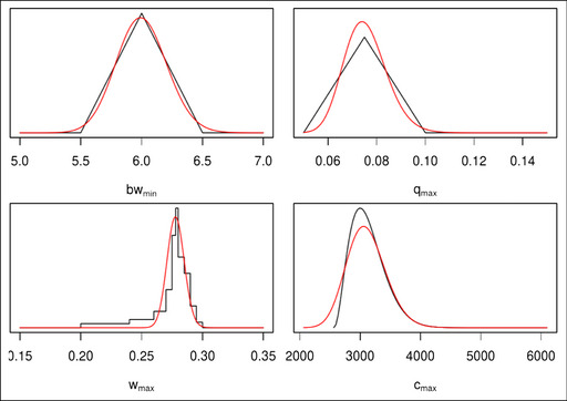
The following figure shows, as a black curve, the probability density function of the distribution representing uncertainty about e_max which was computed, effectively without approximation, by Monte Carlo from the distributions used in Annex B.14. Overlaid in red is the probability density function for the log‐normal distribution calculated above as an approximate representation of uncertainty.

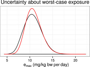
In this example, the approximate probability calculation has resulted in an approximation which performs very well for moderately high percentiles. The figure shows that the approximation performs much less well at lower percentiles and does not reveal the fact that the approximation would lead to much higher estimates of extreme high percentiles than should be obtained from the distributions used in Annex B.14. The approximation might have performed very differently had different choices been made about which percentiles to use as the basis for the original approximations to c_max, w_max, q_max and bw_min or had the shapes of the distributions specified in Annex B.14 been different.

Strengths

1. Simplicity of application.

2. Provides full probability distribution for a combination of uncertainties.

Weaknesses and possible approaches to reduce them

1. Only provides an approximation to the distribution representing combined uncertainty and the accuracy of approximation is difficult to judge and is percentile dependent.

2. Restricted to certain simple models: addition of uncertain components or multiplication of uncertain components but not both at the same time.

3. Distributions, for the individual certainties to be combined, need to be suitable for approximation by normal distributions for uncertain components being added or by log‐normal distributions for components being multiplied.

Assessment against evaluation criteria

This method is assessed against the criteria in Table B.30.

Table B.30.

Assessment of Approximate calculations (when applied well) against evaluation criteria

Criteria	Evidence of current acceptance	Expertise needed to conduct	Time needed	Theoretical basis	Degree/extent of subjectivity	Method of propagation	Treatment of uncertainty and variability	Meaning of output	Transparency and reproducibility	Ease of understanding for non‐specialist
Stronger characteristics	International guidelines or standard scientific method	No specialist knowledge required	Hours	Well established, coherent basis for all aspects	Judgement used only to choose method of analysis	Calculation based on appropriate theory	Different types of uncertainty & variability quantified separately	Range and probability of possible answers	All aspects of process and reasoning fully documented	All aspects fully understandable
	EU level guidelines or widespread in practice	Can be used with guidelines or literature	Days	Most but not all aspects supported by theory	Combination of data and expert judgement	Formal expert judgement	Uncertainty and variability quantified separately	Range and relative possibility of answers	Most aspects of process and reasoning well documented	Outputs and most of process understandable
	National guidelines, or well established in practice or literature	Training course needed	Weeks	Some aspects supported by theory	Expert judgement on defined quantitative scales	Informal expert judgement	Uncertainty and variability distinguished qualitatively	Range of answers but no weighting	Process well documented but limited explanation of reasoning	Outputs and principles of process understandable
	Some publications and/or regulatory practice	Substantial expertise or experience needed	A few months	Limited theoretical basis	Expert judgement on defined ordinal scales	Calculation or matrices without theoretical basis		Quantitative measure of degree of uncertainty	Limited explanation of process and/or basis for conclusions	Outputs understandable but not process
Weaker characteristics	Newly developed	Professional statistician needed	Many months	Pragmatic approach without theoretical basis	Verbal description, no defined scale	No propagation	No distinction between variability and uncertainty	Ordinal scale or narrative description for degree of uncertainty	No explanation of process or basis for conclusions	Process and outputs only understandable for specialists

Conclusions

The method is potentially useful, especially as a quick way to approximately combine uncertainties. However, the fact that the accuracy of the method is generally unknown may limit its usefulness.

References

Gaylor DW and Kodell RL, 2000. Percentiles of the product of uncertainty factors for establishing probabilistic reference doses. Risk Analysis, 20, 245–250.

IPCS (International Programme on Chemical Safety), 2014. Guidance Document on Evaluating and Expressing Uncertainty in Hazard Assessment. IPCS Harmonization Project Document No. 11. World Health Organisation, Geneva. Available online: http://www.inchem.org/documents/harmproj/harmproj/harmproj11.pdf

Krzanowski W, 2000. Principles of multivariate analysis. OUP Oxford.

Rice JA, 2006. Mathematical Statistics and Data Analysis, 3rd Edition. Brooks Cole.

B.16. Deterministic calculations with conservative assumptions

Purpose, origin and principal features

This section addresses a set of related approaches to dealing with uncertainty that involve deterministic calculations using assumptions that aim to be conservative, in the sense of tending to overestimate risk (see also Section 5.8 of Guidance).

A deterministic calculation uses fixed numbers as input and will always give the same answer, in contrast to a probabilistic calculation where one or more inputs are distributions and repeated calculations give different answers.

In deterministic calculation, uncertain elements are represented by single numbers, some or all of which may be conservative. Various types of these can be distinguished:

• default assessment factors such as those used for inter‐ and intraspecies extrapolation in toxicology

• chemical‐specific adjustment factors used for inter‐ or intraspecies differences when suitable data are available

• default values for various parameters (e.g. body weight), including those reviewed by the Scientific Committee (EFSA, 2012)

• conservative assumptions specific to particular assessments, e.g. for various parameters in the exposure assessment for BPA (EFSA, 2015a,b,c)

• decision criteria with which the result of a deterministic calculation is compared to determine whether refined assessment is required, such as the Toxicity Exposure Ratio in environmental risk assessment for pesticides (e.g. EFSA, 2009).

Those described as default are intended for use as a standard tool in many assessments in the absence of specific relevant data. Those described as specific are applied within a particular assessment and are based on data or other information specific to that case. Default factors may be replaced by specific factors in cases where suitable case‐specific data exist.

These are among the most common approaches to uncertainty in EFSA's work. They have diverse origins, some dating back several decades (see EFSA, 2012). What they have in common is that they use a single number to represent something that could in reality take a range of values, and that at least some of the numbers are chosen in a one‐sided way that is intended to make the assessment conservative.

Deterministic calculations generally involve a combination of several default and specific values, each of which may be more or less conservative in themselves. Assessors need to use a combination of values that results in an appropriate degree of conservatism for the assessment as a whole, since that is what matters for decision‐making.

The remainder of this section introduces the principles of this class of approaches, in four steps. The first two parts introduce the logic of default and specific values, using inter‐ and intraspecies extrapolation of chemical toxicity as an example. The third part shows how similar principles apply to other types of default factors, assumptions and decision criteria, and the fourth part discusses the conservatism of the output from deterministic calculations. The subsequent section then provides an overview of how these approaches are applied within EFSA's human and environmental risk assessments.

Default factors for inter‐ and intraspecies differences in toxicity

Default factors for inter‐ and intraspecies differences are used to allow for the possible difference between a specified point of departure from an animal toxicity study and the dose for a corresponding effect in a sensitive human. The size of this difference (expressed as a ratio) varies between chemicals, as illustrated by the distribution in Figure B.16. If there are no specific data on the size of the ratio for a particular chemical, then the size of the ratio for that chemical is uncertain and a default factor is required. The default factor is intended to be high enough that the proportion of chemicals with higher values is small, as illustrated by the grey shaded area in Figure B.16. This default factor is conservative in the sense that, for most chemicals, the true ratio will be lower than the default (white area of distribution in Figure B.16). If the default factor is applied to a particular chemical, there is a high probability that the true ratio for that chemical is lower than the default (i.e. high coverage, see Section 5.8 and IPCS (2014)). Thus, the distribution in Figure B.16 represents variability of the ratio in the population of chemicals, but uncertainty for a single chemical.

Figure B.16.

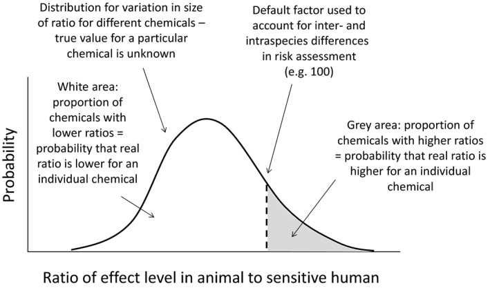
Graphical representation of the general concept for default assessment factors for inter‐ and intraspecies differences in toxicity

The same default value is used for different chemicals in the population because, in the absence of specific data, the same distribution applies to them all. If their true ratios became known, it would be found that the default factor was conservative for some and unconservative for others. However, in the absence of chemical‐specific data, the ratios could lie anywhere in the distribution. Therefore, the same default factor is therefore equally conservative for all chemicals that lack specific data at the time they are assessed.

In order to specify the distribution in Figure B.16, it is necessary to define the starting and ending points for extrapolation. The starting point is generally a NOAEL or BMDL, which are intended to under‐estimate the dose causing effects in animals and thus contribute to making the assessment conservative (see Section 4.2 of IPCS (2014) for discussion of these and also the LOAEL). The ending point for extrapolation is a ‘sensitive human’. This could be defined as a specified percentile of the human population, as in the ‘HDMI’, the human dose at which a fraction I of the population shows an effect of magnitude M or greater, an effects metric proposed by IPCS (2014).

In practice, the distribution for variability between chemicals is not known perfectly: there is at least some uncertainty about its shape and parameters (e.g. mean and variance) which could quantified in various ways (e.g. Bayesian inference, sensitivity analysis or expert judgement, see Sections B.9 and B.16). This uncertainty about the distribution for the population of chemicals adds to the uncertainty for an individual chemical. This can be taken into account by basing the default factor on a single distribution that includes both sources of uncertainty (uncertainty about the shape of the distribution, and about where a given chemical lies within it). In general, this will be wider than the estimated distribution for variability between chemicals, and consequently a larger default factor will be needed to cover the same proportion of cases, i.e. to achieve the same degree of coverage or conservatism. This is illustrated graphically in Figure B.17. If the uncertainty about the distribution is not taken into account within the default factor, then it should either be quantified separately or taken into account in the combined characterisation of identified uncertainties for the assessment as a whole (see Section 14 of main document).

Figure B.17.

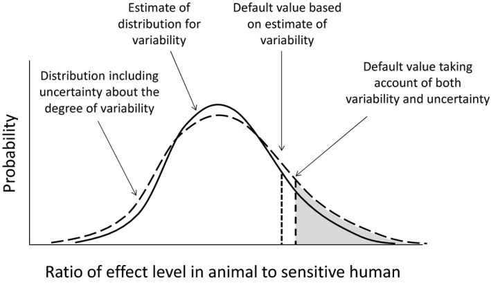
Graphical representation of how uncertainty about the distribution for variability between chemicals can be taken into account when setting a default assessment factor

Specific factors for inter‐ and intraspecies differences in toxicity

When chemical‐specific data are available to reduce uncertainty about part of the extrapolation for inter‐ and intraspecies differences, this can be used to replace the corresponding part of the default assessment factor, as summarised by EFSA (2012a,b,c). The default factor of 100 was introduced in the 1950s and later interpreted as reflecting extrapolation from experimental animals to humans (factor 10 for interspecies variability) and a factor of 10 to cover inter‐individual human variability. A further division of these inter‐ and intraspecies factors into 4 subfactors based on specific quantitative information on toxicokinetics and toxicodynamics was proposed by IPCS (2005). If specific data on toxicokinetics or toxicodynamics are available for a particular chemical, this can be used to derive chemical‐specific adjustment factors (CSAF), which can then be used to replace the relevant subfactor within the overall default factor of 100.

IPCS (2005) provides detailed guidance on the type and quality of data required to derive CSAFs. For the interspecies differences, this includes guidance that the standard error of the mean of the data supporting the CSAF should be less than approximately 20% of the mean. The guidance is designed to limit the sampling and measurement uncertainty affecting the data to a level that is small enough that the mean can be used as the basis for the CSAF.

The treatment of uncertainty for the CSAF is illustrated graphically in Figure B.18. The distribution represents all the uncertainty in deriving the CSAF. The value taken as the CSAF is the mean of the data. If this is near the median of the distribution, as illustrated in Figure B.18, then there is about a 50% chance that the true CSAF is higher. However, the criteria recommended in the guidance to reduce uncertainty mean that the true value is unlikely to be much higher than the mean of the data.

Figure B.18.

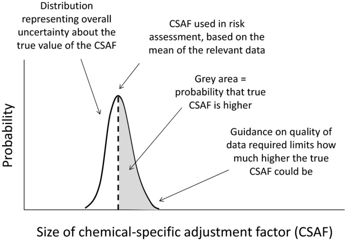
Graphical illustration of treatment of uncertainty for a chemical‐specific adjustment factor for inter‐ or intraspecies differences in toxicokinetics or toxicodynamics

This illustrates an important general point, which is that the choice of an appropriately conservative value to represent an uncertain or variable quantity depends not only on the chance that the true value is higher, but also on how much higher it could be.

Default and specific values for other issues

The principles and logic that are involved when using default or specific factors for inter‐ and intraspecies differences, as illustrated in Figures B.16, B.17 and B.18, apply equally to other types of default and specific values used in risk assessment. This includes default values recommended by the Scientific Committee (EFSA, 2012), some of which refer to toxicity (including inter‐ and intraspecies differences and extrapolation from subchronic to chronic endpoints) while others refer to exposure assessment (e.g. default values for consumption and body weight). For several other issues, EFSA (2012a,b,c) does not propose a default factor but instead states that specific assessment factors should be derived case‐by‐case.

The same principles and logic also apply to all other values used in deterministic assessment, including conservative assumptions (which may be defaults applied to many assessments, or specific to a particular assessment) and decision criteria (which are usually defaults applied to many assessments). For example, in the melamine statement (EFSA, 2008), variability and uncertainty are addressed by repeating the assessment calculation with both central and high estimates for several parameters (described in more detail in the example at the end of this section).

What all of these situations have in common is that, in each assessment calculation, single values – either default or specific or a mixture of both – are used to represent quantities that are uncertain, and in many cases also variable. For each default or specific value, there is in reality a single true value that would allow for the uncertainty and variability that is being addressed. However, this true value is unknown. The degree to which each default or specific value is conservative depends on the probability that the true value would lead to a higher estimate of risk, and how much higher it could be. Figures B.16, B.17 and B.18 illustrate this for the case of parameters that are positively related to risk; for parameters that are negatively related to risk, the grey areas would be on the left side of the distribution instead of the right.

There are two main ways by which default and specific values can be established. Where suitable data are available to estimate distributions quantifying the uncertainty and variability they are intended to address, it is preferable to do this by statistical analysis and then choose an appropriately conservative value from the distribution. Where this is not possible or such data are not available, it is necessary to use expert judgement. In the latter case, the distribution should be elicited by formal or semi‐formal EKE, depending on the importance of the choice and the time and resources available (see Sections B.8 and B.9). Alternatively, if the required degree of conservatism were known in advance, that percentile of the distribution could be elicited directly, without eliciting the full distribution.

It is especially important to ensure the appropriateness of default factors, assumptions and decision criteria, as they are intended for repeated use in many assessments. The context for which they are appropriate must be defined, that is, for what types of assessment problem, with which types and quality of data. When using them in a particular assessment, users must check whether the problem and data are consistent with the context for which the defaults are valid. If the assessment in hand differs, e.g. if the data available differ from those for which the defaults were designed, then the assessors need to consider adjusting the defaults or adding specific factors to adjust the assessment appropriately (e.g. an additional factor allowing for non‐standard data). The need to ensure default procedures for screening assessments are appropriately conservative, and to adjust them for non‐standard cases, was recognised previously in the Scientific Committee's guidance on uncertainty in exposure assessment (EFSA, 2006, 2007).

Combined conservatism of deterministic calculations

Most deterministic assessments involve a combination of default and specific values, each of which may be more or less conservative in themselves. Ultimately, it is the combined conservatism of the assessment as a whole that matters for decision‐making, not the conservatism of individual elements within it. This is why assessors often combine some conservative elements with others that are less conservative, aiming to arrive at an appropriate degree of conservatism overall.

Conservative is a relative term, and can only be assessed relative to a specified objective or target value. Combined conservatism needs to be assessed relative to the quantity the assessment output is intended to estimate, i.e. the measure of risk or other consequence that is of interest to decision‐makers. When the measure of interest is a variable quantity (e.g. exposure), the percentile of interest must also be defined. The combined conservatism of a point estimate produced by deterministic assessment can then be quantified in relation to that target value, as illustrated in Figure B.19.

Figure B.19.

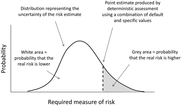
Graphical illustration of assessing the combined conservatism of the output of a deterministic assessment, relative to a specified measure of risk. The distribution is not quantified by the deterministic assessment, so conservatism of the point estimate has to be assessed either by expert judgement, by probabilistic modelling, or by comparison with measured data on risk

Assessing combined conservatism is very hard to do by expert judgement. Although assessors may not think in terms of distributions, judgement of combined conservatism implies considering first what distribution would represent each element, then how those distributions would combine if they were propagated through the assessment – taking account of any dependencies between them – and then what value should be taken from the combined distribution to achieve an appropriate degree of conservatism overall. Finally, the assessors have to choose values for all the individual elements such that, when used together, they produce a result equal to the appropriately conservative point in the combined distribution.

It is much more reliable to assess combined conservatism using probabilistic calculations, when time and resources permit. If it is done by expert judgement, this will introduce additional uncertainty, which the assessors should try to take into account by increasing one or more of the factors involved (in a manner resembling the concept depicted in Figure B.17), or by adding an additional assessment factor at the end.

It is important that the combined degree of conservatism is appropriate: high enough to provide adequate protection against risk, but not so high that the assessment uses clearly impossible values or scenarios or leads to excessively precautionary decision‐making. In terms of Figure B.19, the vertical dashed line should be placed neither too far to the left, nor too far to the right. Achieving this for the final assessment output requires using appropriate values for each default and specific value in the assessment, as explained in the preceding section.

Quantifying the degree of conservatism requires scientific assessment, but deciding what degree of conservatism is required or acceptable is a value judgement which should be made by decision‐makers (see Section 3 of main document). In terms of Figure B.19, characterising the distribution requires scientific consideration, while placing the dashed line requires a value judgement: what probability of acceptable consequences is required? If decision‐makers were able to specify this in advance, assessors could then place the dashed line in Figure B.19 accordingly. Otherwise, assessors will have to choose what level of conservatism to apply when conducting the assessment, and seek confirmation from decision‐makers at the end. In order for decision‐makers to understand the choice they are making, they need information on the probability that the true risk exceeds the estimate produced by the assessment, and on how much higher the true risk might be. In other words, they need information on the uncertainty of the assessment. One of the benefits of establishing defaults is that once approved by decision‐makers, they can be used repeatedly in multiple assessments without requiring confirmation on each occasion.

In refined assessments, default factors or values may be replaced by specific values. This often changes the combined conservatism of the assessment, because that depends on the combined effect of all elements of the assessment (as explained above). Therefore, whenever a default value is replaced by a specific value, the conservatism of the overall assessment needs to be reviewed to confirm it is still appropriate. This issue was recognised previously in EFSA's guidance on risk assessment for birds and mammals (EFSA, 2009).

Applicability in areas relevant for EFSA

Human risk assessment

Default factors, assumptions and decision criteria are, together with descriptive expression, the most common approaches to addressing uncertainty in EFSA and other regulatory agencies, and are used in many areas of EFSA's work. A comprehensive review is outside the scope of this document, but the following examples illustrate the range of applications involved.

Default assessment factors (AFs) and chemical‐specific adjustment factors for inter‐ and intraspecies extrapolation of chemical toxicity are described earlier in this section, and are key tools in setting health‐based guidance values for human health (e.g. TDI and ADI). In recent years, efforts have been made to evaluate the conservatism of the default factors based on analysis, for suitable data sets, of interchemical variability for particular extrapolation steps (e.g. Dourson and Stara, 1983, Vermeire et al. 1999). More recently, it has been proposed (e.g. Cooke, 2010) to do a fully probabilistic analysis of uncertainty about such variability in order to derive default assessment factors. IPCS (2014) have developed a probabilistic approach to inter‐ and intraspecies extrapolation that quantifies the conservatism of the default factors, and includes options for chemical‐specific adjustments. The Scientific Committee has recommended that probabilistic approaches to assessment factors for toxicity are further investigated before harmonisation is proposed within EFSA (2012a,b,c).

Factors and assumptions for other aspects of human health assessment, including exposure, are reviewed by EFSA (2012a,b,c). Topics considered include body weight, food and liquid intake, conversion of concentrations in food or water in animal experiments to daily doses, deficiencies in data and study design, extrapolation for duration of exposure, the absence of a NOAEL, the severity and nature of observed effects and the interpretation of Margins of Exposure for genotoxic carcinogens. EFSA (2012a,b,c) recommends the use of defaults for some of these issues, and case‐by‐case assignment of specific factors for others.

An example of an exposure assessment where the combined conservatism of case‐specific assumptions was explicitly assessed is provided by the 2015 opinion on bisphenol A. Deterministic calculations were aimed at estimating an approximate 95th percentile for each source of exposure by combining conservative estimates for some parameters with average estimates for others. The uncertainty of these, and their combined impact on the combined conservatism of the resulting estimate, was assessed by expert judgement using uncertainty tables (EFSA, 2015a).

An example of probabilistic analysis being used to evaluate the conservatism of default assumptions in human exposure assessment is provided by EFSA (2007). This used probabilistic exposure estimates for multiple pesticides and commodities to evaluate what proportion of the population are protected by the deterministic ‘IESTI’ equations used in routine exposure assessment.

Environmental risk assessment

Default factors for interspecies differences, similar to those used for human risk, have been used for some time in setting environmental standards for ecosystems such as the predicted no effect concentration (PNEC). In some guidance documents for environmental risk assessment, a reference point from toxicity testing is divided by a default assessment factor and the result compared to the predicted exposure by computing their ratio, which is known as the risk quotient (RQ) (European Commission, 2003). In others the reference point is first divided by the predicted exposure to find the toxicity–exposure ratio (TER) and the result is then compared to a decision criterion, which is equivalent to an assessment factor (91/414/EWG). Although the calculations appear different, they lead to the same result and it is clear from the reasoning in the respective guidance documents that the assessment factors are intended to address variability and uncertainties relating to toxicity.

Most environmental exposure assessments are deterministic, using a combination of conservative factors and assumptions, some of which are defaults and some specific. Examples of these include the Tier 1 procedures for assessing acute and reproductive risks from pesticides to birds and mammals, which define different combinations of default assumptions to be used for different species that may be exposed, depending on the type of pesticide use involved. The guidance includes the option to replace the defaults with specific assumptions in refined assessment, where justified (EFSA, 2009). In assessing exposure of aquatic organisms to pesticides, a range of ‘FOCUS’ scenarios with differing defaults are used, representing different combinations of environmental conditions found in different parts of the EU (FOCUS, 2001).

As for human risk, some quantitative analyses have been conducted to justify or calibrate the defaults used in environmental risk. When developing the current guidance on pesticide risk assessment for birds and mammals, the procedure for acute risk to birds was calibrated by comparison with data on bird mortality in field experiments and history of use, as well as assessing its conservatism by expert judgement. For acute risk to mammals and reproductive risks, field data were lacking and it was necessary to rely on expert judgement alone (EFSA, 2008). For aquatic organisms, factors for extrapolating from laboratory toxicity studies with individual species to effects on communities of multiple species have been calibrated by comparing results from single species tests with semi‐field experiments (Maltby et al., 2009; Wijngaarden et al., 2014). As for human risk, it has been proposed that, in future, default factors used in environmental risk assessment should be derived from a fully probabilistic analysis taking both variability and uncertainty into account (EFSA, 2015a,b,c).

Potential contribution to major elements of uncertainty analysis

Elements in uncertainty analysis	Potential contribution of this approach
Identifying uncertainties	Not applicable. However, by discussing the need for assessment factor(s) you also identify some uncertainties
Characterising uncertainties	Yes, for uncertainties represented by assessment factors
Combining uncertainties	Yes. Decision criteria, some assessment factors, and the results of calculations with conservative assumptions are designed to address the combined effect of multiple uncertainties. The way they are used implies that they account for dependencies, though this is rarely explicit
Prioritising uncertainties	In assessments that include multiple assessment factors, their magnitudes should reflect the assessors’ evaluation of their relative importance

Melamine example

In this document, the case study of melamine as described in EFSA (2008) is used to illustrate the different approaches to assessing uncertainty. In EFSA (2008), a TDI set by the SCF (European Commission, 1986) was used. Since that document does not describe the RP and the AFs used for deriving the TDI, an example of the use of assessment factors for toxicity is taken from an assessment made by the US‐FDA (FDA, 2007), which is also referenced by EFSA (2008). The following quote from FDA (2007) explains how the TDI was derived from combining a point of departure based on a detailed evaluation of toxicity studies with default assessment factors for inter‐ and intraspecies extrapolation:

‘The NOAEL for stone formation of melamine toxicity is 63 mg/kg bw per day in a 13‐week rat study. This value is the lowest NOAEL noted in the published literature and is used with human exposure assessments below to provide an estimate of human safety/risk… This PoD was then divided by two 10‐fold safety/uncertainty factors (SF/UF) to account for inter‐ and intra‐species sensitivity, for a total SF/UF of 100. The resulting Tolerable Daily Intake (TDI) is 0.63 mg/kg bw per day. The TDI is defined as the estimated maximum amount of an agent to which individuals in a population may be exposed daily over their lifetimes without an appreciable health risk with respect to the endpoint from which the NOAEL is calculated’.

The exposure assessment in the EFSA (2008) statement addressed variability and uncertainty by estimating exposure for a range of scenarios using different combinations of assumptions, with varying degrees of conservatism. The factors that were varied included age and body weight (60‐kg adult or 20‐kg child), diet (plain biscuit, filled biscuit, quality filled biscuit, milk toffee, chocolate; plus two combinations of biscuit and chocolate), assumptions regarding the proportion of milk powder used in producing each food, and the concentration of melamine in milk powder (median or maximum of reported values). An estimate of exposure was calculated for each scenario, and expressed as a percentage of the TDI of 0.5 mg/kg taken from the SCF assessment (European Commission, 1986). The results are reproduced in Table B.31.

Table B.31.

Exposure estimates for different combinations of assumptions, expressed as a percentage of the TDI of 0.5 mg/kg (reproduced from EFSA, 2008)

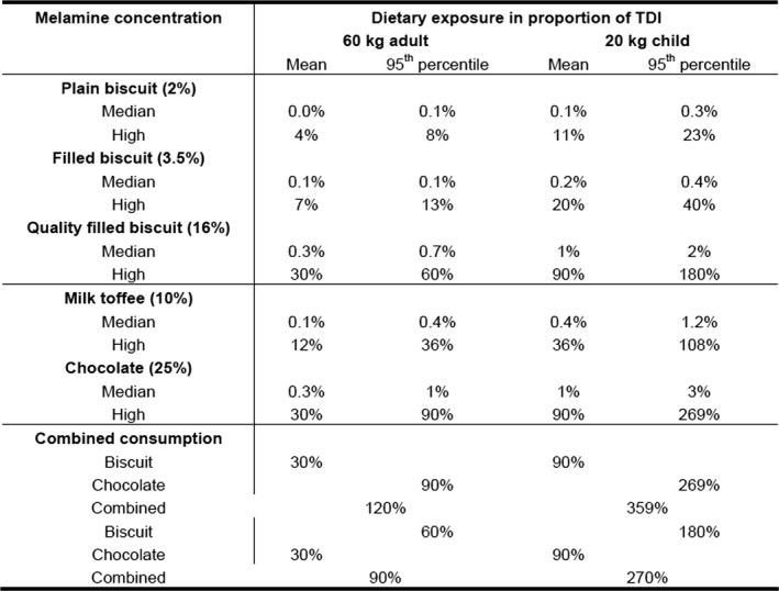
The estimates in Table B.31 involve additional assumptions and uncertainties, some of which are likely to be conservative. For example, EFSA (2008) notes that the calculation involving quality filled biscuits might be a gross overestimation since there was no indication that China exported such products to Europe at that time, though it could not be completely excluded. The chocolate scenario was considered more realistic.

For adults, EFSA (2008) concluded that:

‘Based on these scenarios, estimated exposure does not raise concerns for the health of adults in Europe should they consume chocolates and biscuits containing contaminated milk powder’.

This implies a judgement by the assessors that, although the estimated adult exposures exceeded the TDI in one scenario (mean consumption of biscuit combined with high level consumption of chocolate), overall – considering the probability of this scenario, the combined conservatism of the assumptions made, and the impact of other uncertainties identified in the text – the probability of adverse effects was sufficiently low not to ‘raise concerns’. This could be made more transparent by specifying the assessors’ judgement of level of probability.

For children, EFSA (2008) concluded that:

‘Children with a mean consumption of biscuits, milk toffee and chocolate made with such milk powder would not exceed the tolerable daily intake (TDI). However, in worst case scenarios with the highest level of contamination, children with high daily consumption of milk toffee, chocolate or biscuits containing high levels of milk powder would exceed the TDI. Children who consume both such biscuits and chocolate could potentially exceed the TDI by more than threefold. However, EFSA noted that it is presently unknown whether such high level exposure scenarios may occur in Europe’.

The conclusion for children is more uncertain than for adults. The assessors state that the exposure could ‘potentially’ exceed the TDI by more than threefold in one scenario, but do not express a judgement on how likely that is to occur.

Strengths

1. Conservative assessment factors, assumptions and decision criteria address uncertainty using a one‐sided approach that aims to be conservative but not over‐conservative.

2. The methodology is widely adopted, well accepted by authorities, and easy to communicate.

3. It can be used in any type of quantitative assessment.

4. Once established, default factors are straightforward to apply and do not require any special mathematical or statistical skills.

5. Some default factors and criteria are supported by quantitative analysis of data that supports their appropriateness for their intended use. Similar analyses could be attempted for others, where suitable data exist.

Weaknesses and possible approaches to reduce them

1. While some default assessment factors are generally well‐accepted and research has provided quantitative support, the use of other default factors and most specific factors is based mainly on expert judgement without quantitative detail and it can be difficult to establish either the reasoning that led to a particular value or exactly what sources of uncertainty are included.

2. Generation of specific factors, and providing quantitative support for default factors where this is currently lacking, require relevant expertise to evaluate the available evidence and statistical expertise for analysis.

3. Assessment factors which are based on analysis of data without quantification of uncertainty about variability may be less conservative than intended (as illustrated in Figure B.17).

4. It is often unclear how conservative the result is intended to be. This could be addressed by defining more precisely what extrapolation or adjustment is being made and what level of confidence is required, in consultation with decision‐makers.

5. There is little theoretical basis for assuming that assessment factors should be multiplied together, as is often done. However such multiplication tends to contribute to the conservatism of the approach (Gaylor and Kodell, 2000). Annex B.13 of this annex on probability bounds provides a rationale for multiplication if a probability is attached to each individual AF.

6. Division of AFs into subfactors could lead to reduced conservatism if, for example, a CSAF greater than the default subfactor is needed to cover a particular source of variability. The reduction of conservatism could be quantified by a probabilistic analysis.

7. As a consequence of the above issues, different hazard characterisations (related to different chemicals) may differ widely in the level of conservatism, depending on the number of assessment factors used and the values used for them.

8. AFs do not provide a range for the quantity of interest, based on the propagation of the uncertainty around the various input factors, but only a conservative estimate of the quantity of interest.

9. Risk management decisions, about the level of conservatism required, are embedded in the AF. For the process to be transparent, such decisions need to be made explicit.

10. Assessment factors do not generally provide a mechanism to assess the relative contribution of different sources of uncertainty to overall uncertainty or to distinguish contributions of variability and uncertainty. A probabilistic analysis can provide a general indication of relative contributions for the selected group of chemicals.

Assessment against evaluation criteria

This method is assessed against the criteria in Table B.32.

Table B.32.

Assessment of Deterministic calculations with conservative assumptions (when applied well) against evaluation criteria

Criteria	Evidence of current acceptance	Expertise needed to conduct	Time needed	Theoretical basis	Degree/extent of subjectivity	Method of propagation	Treatment of uncertainty and variability	Meaning of output	Transparency and reproducibility	Ease of understanding for non‐specialist
Stronger characteristics	International guidelines or standard scientific method	No specialist knowledge required	Hours	Well established, coherent basis for all aspects	Judgement used only to choose method of analysis	Calculation based on appropriate theory	Different types of uncertainty & variability quantified separately	Range and probability of possible answers	All aspects of process and reasoning fully documented	All aspects fully understandable
	EU level guidelines or widespread in practice	Can be used with guidelines or literature	Days	Most but not all aspects supported by theory	Combination of data and expert judgement	Formal expert judgement	Uncertainty and variability quantified separately	Range and relative possibility of answers	Most aspects of process and reasoning well documented	Outputs and most of process understandable
	National guidelines, or well established in practice or literature	Training course needed	Weeks	Some aspects supported by theory	Expert judgement on defined quantitative scales	Informal expert judgement	Uncertainty and variability distinguished qualitatively	Range of answers but no weighting	Process well documented but limited explanation of reasoning	Outputs and principles of process understandable
	Some publications and/or regulatory practice	Substantial expertise or experience needed	A few months	Limited theoretical basis	Expert judgement on defined ordinal scales	Calculation or matrices without theoretical basis		Quantitative measure of degree of uncertainty	Limited explanation of process and/or basis for conclusions	Outputs understandable but not process
Weaker characteristics	Newly developed	Professional statistician needed	Many months	Pragmatic approach without theoretical basis	Verbal description, no defined scale	No propagation	No distinction between variability and uncertainty	Ordinal scale or narrative description for degree of uncertainty	No explanation of process or basis for conclusions	Process and outputs only understandable for specialists

Conclusions

Assessment factors, conservative assumptions and decision criteria are widely used to account for uncertainty, variability and extrapolation in many areas of EFSA assessment. Some are defaults that can be used in many assessments, while others are specific to particular assessments. They are simple to use and communicate. When well specified and justified they are a valuable tool, providing an appropriate degree of conservatism for the issues they address. They are more reliable when it is possible to calibrate them by statistical analysis of relevant data.

Most assessments involve a combination of multiple factors and assumptions, some default and some specific. Conservatism needs to be evaluated for the assessment as a whole, taking account of all the elements involved. Assessing the combined effect of multiple factors and assumptions is much more reliable when done by probabilistic analysis than by expert judgement.

In order to be transparent and avoid implying risk management judgements, the degree of conservatism needs to be quantified and agreed with decision‐makers. This can be done by providing a probability or approximate probability that the result of the calculation is conservative relative to the quantity of interest. For deterministic calculations that are part of a standardised procedure, this should be done when calibrating the procedure (Section 7.1.3). Where deterministic calculations are used in case‐specific or urgent assessments, their conservatism could be quantified by expert judgement when characterising overall uncertainty, or the deterministic calculation could be replaced by a probability bounds analysis.

References

Cooke R, 2010. Conundrums with Uncertainty Factor (with discussion), Risk Analysis, 30, 330–338.

Dourson ML and Stara JF, 1983. Regulatory History and Experimental Support of Uncertainty (Safety) Factors, Regulatory Toxicology and Pharmacology, 3, 224–238.

European Commission, 1986. Report of the Scientific Committee for Food on certain monomers of other starting substances to be used in the manufacture of plastic materials and articles intended to come into contact with foodstuffs. Seventeenth series. Opinion expressed on 14 December 1984. Available online: http://ec.europa.eu/food/fs/sc/scf/reports/scf_reports_17.pdf

European Commission, 2003. Technical Guidance Document on Risk Assessment. In support of Commission Directive 93/67/EEC on Risk Assessment for new notified substances Commission Regulation (EC) No 1488/94 on Risk Assessment for existing substances Directive 98/8/EC of the European Parliament and of the Council concerning the placing of biocidal products on the market. Part II, Chapter 3 Environmental Risk Assessment.

EFSA (European Food Safety Authority), 2005. Scientific opinion on a request from EFSA related to a harmonised approach for risk assessment of substances which are both genotoxic and carcinogenic. EFSA Journal 2005; 282, 1–31. http://www.efsa.europa.eu/sites/default/files/scientific_output/files/main_documents/282.pdf

EFSA PPR Panel (Panel on Plant protection products and their Residues), 2008. Scientific Opinion on the Science behind the Guidance Document on Risk Assessment for birds and mammals. EFSA Journal 2008; 734, 1–181.

EFSA, (European Food Safety Authority), 2009. Guidance Document on Risk Assessment for Birds and Mammals. EFSA Journal 2009; 7(12):1438. https://doi.org/10.2903/j.efsa.2009.1438

EFSA Scientific Committee, 2012. Guidance on selected default values to be used by the EFSA Scientific Committee, Scientific Panels and Units in the absence of actual measured data. EFSA Journal 2012;10(3):2579. [32 pp.] https://doi.org/10.2903/j.efsa.2012.2579

EFSA CEF Panel (EFSA Panel on Food Contact Materials, Enzymes, Flavourings and Processing Aids), 2015a. Scientific Opinion on the risks to public health related to the presence of bisphenol A (BPA) in foodstuffs: Part I – Exposure assessment. EFSA Journal 2015;13(1):3978, 396 pp. https://doi.org/10.2903/j.efsa.2015.3978 http://www.efsa.europa.eu/sites/default/files/scientific_output/files/main_documents/3978part1.pdf

EFSA PPR Panel (EFSA Panel on Plant Protection Products and their Residues), 2015. Scientific Opinion addressing the state of the science on risk assessment of plant protection products for non‐target arthropods. EFSA Journal 2015;13(2):3996, 212 pp. https://doi.org/10.2903/j.efsa.2015.3996

FDA (United States Food and Drug Administration), 2007. Interim Safety and Risk Assessment of Melamine and its Analogues in Food for Humans. Available online: http://www.fda.gov/food/foodborneillnesscontaminants/chemicalcontaminants/ucm164658.htm [Accessed: 13 March 2015].

FOCUS (2001). “FOCUS Surface Water Scenarios in the EU Evaluation Process under 91/414/EEC”. Report of the FOCUS Working Group on Surface Water Scenarios, EC Document Reference SANCO/4802/2001‐rev.2. 245 pp.

Gaylor DW and Kodell R, 2000. Percentiles of the Product of Uncertainty Factors for Establishing Probabilistic Reference Doses, Risk Analysis, 20, 245–250.

IPCS, 2005. Chemical‐specific adjustment factors for interspecies differences and human variability: guidance document for use of data in dose/concentration–response assessment. IPCS Harmonization Project Document No. 2. World Health Organisation, Geneva.

IPCS, 2014. Guidance document on evaluating and expressing uncertainty in hazard characterization. Harmonization Project Document No. 11. International Programme on Chemical Safety. WHO, Geneva.

Maltby L, Brock TCM and Brink PJ, 2009. Fungicide risk assessment for aquatic ecosystems: importance of interspecific variation, toxic mode of action, and exposure regime. Environmental Science Technology, 43, 7556–7563.

Vermeire T, Stevenson H, Pieters M., Rennen M, Slob W and Hakkert BC, 1999. Assessment factors for human health risk assessment: a discussion paper, Critical Reviews in Toxicology, 29, 439–490.

van Wijngaarden RPA, Maltby L and Brock TCM 2014. Acute tier‐1 and tier‐2 effect assessment approaches in the EFSA Aquatic Guidance Document: are they sufficiently protective for insecticides? In press. https://doi.org/10.1002/ps.3937

B.17. Sensitivity analysis

Purpose, origin, and principal features

In the context of uncertainty analysis, sensitivity analysis aims to identify both the magnitude of the contributions of individual sources of uncertainty to uncertainty about the assessment output(s) and the relative contributions of different sources. The purpose of doing so is (i) to help prioritise uncertainties for quantification: (ii) to help prioritise uncertainties for collecting additional data; (iii) to investigate sensitivity of final output to assumptions made; (iv) to investigate robustness of final results to assumptions made.

Saltelli et al. (2004) defines sensitivity analysis of a model as ‘the study of how uncertainty in the output of a model (numerical or otherwise) can be apportioned to different sources of uncertainty in the model input’. A broader definition of Sensitivity Analysis is given in the Oxford business dictionary where it is described as ‘Simulation analysis in which key quantitative assumptions and computations (underlying a decision, estimate, or project) are changed systematically to assess their effect on the final outcome. Employed commonly in evaluation of the overall risk or in identification of critical factors, it attempts to predict alternative outcomes of the same course of action’. According to Saltelli, desirable properties of a sensitivity analysis method for models include the ability to cope with influence of scale and shape; the allowance for multidimensional averaging (all factors should be able to vary at the same time); model independence (i.e. the method should work regardless of additively or linearity of the model); ability to treat grouped factors as if they were single factors.

There is a very large and diverse literature on sensitivity analysis reflecting the fact that historically sensitivity analysis methods have been widely used across various disciplines including engineering systems, economics, physics, social sciences and decision making. Saltelli et al. (2004, 2008) provide an overview of the various methods available and Frey and Patil (2002) and Patil and Frey (2004) review and compare methods in the context of food‐safety risk assessment. Most of the literature deals with the use of sensitivity analysis methods in the presence of a model.

Two general approaches to sensitivity analysis have been developed. The first approach looks at the effects on the output of infinitesimal changes to the default values of the inputs (local) while the second one investigates the influence on the output of changes of the inputs over their whole range of values (global). In the following, the discussion will focus only on methods for global sensitivity analysis since local analysis is considered of limited relevance in the uncertainty analysis context because it does not provide for an exploration of the whole space of the input factors that is necessary when dealing with uncertainty. Whatever the context, it is important that the purpose of sensitivity analysis is clearly defined after consideration and, when needed, prioritisation of the inputs to be included in the sensitivity analysis.

One special type of sensitivity analysis is conditional sensitivity analysis which is sometimes considered to be a form of scenario analysis. It is generally helpful when there is a dependency in the inputs and it is difficult to assess the sensitivity of the output to changes in a single input without fixing some prespecified values of the other inputs. Conditional sensitivity analysis expresses the sensitivity of the output to one input, with other inputs kept constant at prespecified values (values considered more likely or of special interest). The most common approach in conditional sensitivity analysis is to combine key variables making reference to three possible cases: (a) worst‐case or conservative scenario; (b) most likely or base scenario; (c) best‐case or optimistic scenario.

Frey and Patil (2002) suggest grouping methodologies for sensitivity analysis in three categories: mathematical methods, statistical methods, graphical methods. These categories could be further classified according to other important aspects such as the kind of input effects that they are able to capture (individual or joint) and the form of the relationship between inputs and output (linear or non‐linear). A comparison of the main methodologies and their most appropriate use in relation to the objective of the sensitivity analysis is provided by the same authors. Only those methods that are deemed to be relevant in the framework of uncertainty analysis and applicable to the risk assessment context are described in this section. Therefore, the list of methods that follows is not comprehensive. Different methods and sensitivity indexes can provide a range of different factor rankings. Where this happens, the assessors need to consider the cause of the differences and their implications for interpretation of the results.

A summary of the methods considered in this document for sensitivity analysis are provided in Table B.33.

Table B.33.

Summary table of methods to perform sensitivity analysis

Group	Method	Acronym	Characteristics
Graphical	Tornado plot		Input factors sorted by their influence on the output in a decreasing order
	Scatter plot		Highlight relationship between output and each input factor. No interaction among factors
	Spider plot		Plot all the input factors as lines crossing at the nominal value of the output. The inputs with the highest slope are those with highest influence on the output
	Box plot		Range of variation of the output with respect to each input
	Pie chart		Split of the pie in slices whose size is proportional to the influence of each input
Mathematical/deterministic	Nominal Range Sensitivity Analysis	NRSA	No interaction among input factors, monotonic relationship
	Difference of log odds ratio	ΔLOR	Special case of NRSA when output is a probability
	Break‐even analysis	BEA	Output is a dichotomous variable
Probabilistic	Morris	Morris	Qualitative screening of inputs
	Monte Carlo filtering	MCF	Analogous of BEA with probabilistic approach
	Linear rank regression analysis	SRC, SRRC, PCC, PRCC.	Strong assumptions: normality residuals, uncorrelation among inputs, linear relationship
	Analysis of Variance	ANOVA	Non parametric method
	Fourier Amplitude Sensitivity Test and Extended version	FAST, E‐FAST	Variance‐base method. No assumptions required.
	Sobol index	S	Widely applicable

Graphical methods

These are normally used to complement mathematical or statistical methodologies especially to represent complex dependency and facilitate their interpretation. They are also used in the early stage to help prioritising among sources of uncertainty. Graphical methods include: scatterplot, tornado plots, box plots, spider plots and pie charts (Patil and Fray, 2004). In the context of this document, they are considered only as supporting methods to help interpretation of the sensitivity analysis results. Examples of graphical methods for sensitivity analysis are provided in Figure B.20.

Figure B.20.

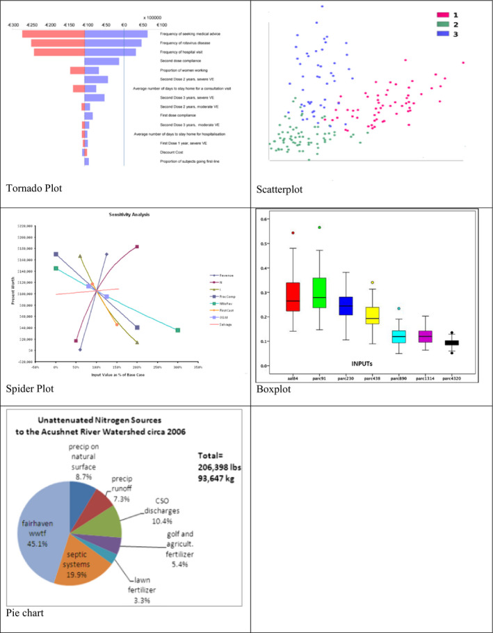
Examples of graphical methods for sensitivity analysis

Deterministic (named ‘mathematical’ by Patil & Frey) methods

These methods involve evaluating the variability of the output with respect to a range of variation of the input with no further consideration of the probability of occurrence of its values. For this reason and to keep the symmetry with the classification adopted for the uncertainty analysis approaches, they are referred to as ‘deterministic’ instead of mathematical methods. In case of monotonic relationship, these methods can be useful for a first screening of the most influential inputs. Graphical methods and the revised Morris method are suitable alternatives when monotonicity is not met.

• 1Nominal range sensitivity analysis (NRSA)

This method is normally applied to deterministic models (Cullen and Frey 1999). It assesses the effect on the output of moving one input from its nominal (often most‐likely) value to its upper and lower most extreme plausible values while keeping all the other inputs fixed at their nominal values. The resulting sensitivity measure is the difference in the output variable due to the change in the input (expressed sometimes as percentage). The method of ‘minimal assessment’, proposed by EFSA (2014a,b) for prioritising parameters for formal expert elicitation, is an example of nominal range sensitivity analysis.

This approach to sensitivity analysis is closely related to interval analysis (see Annex B.7).

Interactions among factors are not accounted for by this method which limits its capacity to estimate true sensitivity. Although simple to implement, it fails in case of non monotonic relationships because it does not examine behaviour in for input values between the extremes.

A specific case of the nominal range is the difference of log odds ratio which can be used in case of an output expressed as probability. It is based on the computation of the log‐odds or log‐odds‐ratio of an event.

• 2Break‐even analysis (BEA)

The purpose of this method is to identify a set of values of inputs (break‐even values) that provide an output for which decision‐makers would be indifferent among the various risk management options (Patil and Fray, 2004). This method is useful to assess the robustness of a decision to change in inputs (i.e. whether a management option still remains optimal or suboptimal also in case the values of inputs change with respect to the current levels). It is commonly used when the output is expressed as dichotomous variable indicating two possible options such as whether a tolerable daily intake is exceeded or not. It represents a useful tool for evaluating the impact of uncertainty on different possible choices of policy maker (e.g. what level of use to permit for a food additive).

The BEA has a probabilistic counterpart in Monte Carlo filtering which partitions the outputs in two sets based on compliance/non‐compliance with some criterion (see later).

Statistical methods

In statistical methods of sensitivity analysis, the input range of variation is addressed probabilistically so that not only different values of the inputs but also the probability that they occur are considered in the sensitivity analysis. This approach to the sensitivity analysis is naturally linked to the investigation of the uncertainty based on probabilistic methods.

Most of the methods belonging to this group are based on the decomposition of the output variance with respect to the variability of the inputs. They generally allow the assessors to identify the effect of interactions among multiple inputs. Frequently statistical sensitivity analysis is performed using Monte Carlo techniques (sometimes combined with bootstrapping techniques),although this approach is not strictly necessary and sometimes not preferable if it is too computationally intensive.

Identification of the separated influence of variability and uncertainty in the input on the uncertainty in the output is not a trivial issue in sensitivity analysis. Recently, Busschaert et al. (2011) proposed an advanced sensitivity analysis to address this issue. This analysis is sometimes referred to as two‐dimensional sensitivity analysis. It is not described in detail in this document. A simple, limited, approach to sensitivity analysis in assessments which involve uncertainty about variability is to identify a percentile of variability which is of interest and to make an analysis of the sensitivity of the estimate of that percentile to uncertainty about input parameters.

• 1Morris method

The Morris method provides a qualitative measure of the importance of each uncertain input factor for the outputs of a model at a very low computational cost, determining factors that have: (i) negligible effects; (ii) linear and additive effects (iii) non‐linear and/or non‐additive effects (Saltelli et al., 2005). The methods can be used as a qualitative screening procedure to select the most important input factors for computationally more demanding variance‐based methods for sensitivity analysis. The Morris method varies one factor at a time across a certain number of levels selected in the space of the input factors. For each variation, the factor's elementary effect is computed, which measures, relative to the size of the change, how much the output changed when the factor value was changed.

The number of computations required is N = T (k + 1), where k is the number of model input factors and the number of sampling trajectories T is a number generally ranging between 10 and 20 depending on the required accuracy. Ten trajectories are usually considered sufficient (Saltelli et al., 2004). Different sampling methods are available. Khare et al. (2015) describe a new sampling strategy (sampling for uniformity (SU)), which was found to perform better than existing strategies using a number of criteria including: generated input factor distributions’ uniformity, time efficiency, trajectory spread, and screening efficiency. We use the SU method in the example that follows on melamine.

The mean of the elementary effects for a factor estimates the factor's overall effect (μ_i). A high value suggests a strong linear effect of that factor, whereas a high value of the standard deviation of the elementary effects (σ_i) indicates a non‐linear or non‐additive effect. For non‐monotonic effects, the mean of the absolute values of the elementary effects can also be computed to avoid cancelling out of opposing signals (Saltelli et al., 2005). When using absolute values the method is known as revised Morris. Visualisation is possible by plotting the mean elementary effect for each factor versus the standard deviation. Input factors which have large mean or standard deviation of the elementary effects (or moderately large values of both) are most influential on the model output.

• 2Monte Carlo filtering (MCF)

The goal of MCF is to identify the ranges of these input factors which result in model output which is considered acceptable by decision‐makers (Chu‐Agor et al., 2012). In MCF, a set of constraints has to be defined that targets the desired characteristics of the model realisation (e.g. a threshold value for the risk ratio, set by risk managers or stakeholders). Based on the results of the uncertainty analysis, model results (for example, output values of r) are then classified as being ‘favourable’ or ‘unfavourable’. The values of the input factors are then divided into two groups: those which produce favourable output and those which produce unfavourable output. In order to check what drives the difference between a favourable output and an unfavourable output, a two‐sided Smirnov test is performed for each factor to test if the distribution of the factor is different in the favourable output group than in the unfavourable output group. If the null hypothesis is rejected, this indicates that the input factor is a key factor in driving the model towards favourable outputs, and is a good candidate for risk management intervention. If the null‐hypothesis is accepted, this indicates that at any value of the input factor can result in either a favourable or an unfavourable result, and intervening on that factor is not likely to result in changes in the output of the system represented by the model. In addition to the statistical significance, it is important to evaluate the ranges of input factors that produce differential outputs to explore the biological significance of the findings.

• 3Linear rank regression analysis

The linear regression analysis can be used as a statistical method for investigating sensitivity when it is reasonable to assume that the relationship between inputs and output is linear (Saltelli et al., 2008). A variety of indicators can be computed using this broad approach. The magnitude of the regression coefficients, standardised by the ratio of the standard deviations of model independent and dependent variables (SRC: standardised regression coefficient) is commonly used as a measure of sensitivity as well as the rank assigned to the inputs once sorted by their SRC (SRRC: standardised rank regression coefficient).

$$\text{SRC}={\mathrm{b}}_{\mathrm{i}}·\frac{\text{stddev}({\mathrm{X}}_{\mathrm{i}})}{\text{stddev}(\mathrm{Y})}$$

The partial correlation coefficient (PCC) and the partial rank correlation coefficient (PRCC) can be used alternatively.

The square of the multiple correlation coefficient (R2) is an indicator of goodness of fit of a linear model. Its incremental change, when performing a multivariate stepwise regression analysis, expresses the additional component of variation of the dependent variable explained by the newly introduced input. In the phase of setting up a model, it can be used as a measure of sensitivity to screen factors most influential on the dependent variables.

Possible drawbacks of this class of indicators are the low robustness of the results of regression analysis when key assumptions are not met (e.g. independence of inputs, normality of residuals). In addition these methods are dependent on the functional form (underlying model) explaining the relationship between output and inputs and the range of variation considered for each input.

• 4Analysis of variance

The ANOVA is a sensitivity analysis method that does not require specification of a functional form for the relationship between the output and a set of inputs (non parametric method). The ANOVA aims at investigating whether the variation of the values of the output is significantly associated with the variation of one or more inputs.

• 5Fourier amplitude sensitivity test (FAST)

The FAST method belongs to the class of variance‐based global sensitivity analysis methods. The effect of the uncertain inputs on the output is computed as the ratio of the conditional variance (variance of the conditional distribution of the output having fixed the value of one input or of a combination of inputs) to the total variance of the output. It takes his name from the multiple Fourier series expansion that is used as a tool for computing the conditional variance. The method has a wide applicability since it does not require any assumptions on the model structure nor on monotonicity. In its original form the FAST method (Cukier et al., 1973) required the assumption of no interaction among inputs. Saltelli et al. (1999) developed an extended FAST method that allows accounting for multiple interactions.

Based on Fourier expansion, the total variance of the output can be expressed as the sum of all conditional variances of various orders (from the 1st to the nth):

$$\mathrm{V}=\sum _{\mathrm{j}=1}^{\mathrm{n}}{\mathrm{V}}_{\mathrm{j}}+\sum _{\mathrm{j}=1}^{\mathrm{n}-1}\sum _{\mathrm{k}=\mathrm{j}+1}^{\mathrm{n}}{\mathrm{V}}_{\mathrm{jk}}+\dots +{\mathrm{V}}_{12\dots \mathrm{n}}$$

The first order sensitivity index is computed as the ratio of a single input conditional variance and the total variance whereas the multiple effect sensitivity index is a similar ratio obtained using the multiple factors conditional variance in the numerator.

$${\mathrm{S}}_{{\mathrm{j}}_1{\mathrm{j}}_2\dots {\mathrm{j}}_{\mathrm{r}}}=\frac{{\mathrm{V}}_{{\mathrm{j}}_1{\mathrm{j}}_2\dots {\mathrm{j}}_{\mathrm{r}}}}{\mathrm{V}}$$

Higher values of the index indicate a great influence of the factor/s on the output.

• 6Sobol Index

Sobol's index (Sobol, 1990) is based on the idea of decomposing the output variance into the contributions associated with each input factor. It expresses the reduction in the output variability that could be achieved if value of an input factor was fixed.

The first‐order Sobol index for an input factor is defined as the ratio of the variance of the conditional means of the output (given all possible values of a single input) over the total variance of the output. It indicates the rate of the total output's variance exclusively attributable to a specific input. It does not account for the interaction with other factors.

$${\mathrm{S}}_{\mathrm{j}}=\frac{\mathrm{V}\lfloor \mathrm{E}{\text{(Y/X}}_{\mathrm{j}})\rfloor }{\text{V(Y)}}.$$

In a perfectly additive model the sum of first order sensitivity indices over all the input factors equals 1. Models with a sum greater than 0.6 are considered mostly additive (Saltelli et al., 2004).

The higher order interaction terms express the amount of variance of the output explained by the interaction among factors not already accounted for by lower interaction terms (including first order). It is computed as the ratio of the higher order conditional variance over the total variance of the output.

The total sensitivity index (Homma and Saltelli 1996) of an input is obtained as the sum of the first‐order index and all the higher order interaction terms involving that specific input.

Traditionally the computation of the Sobol indexes is performed running simulations with the Monte Carlo algorithm. The computational requirements of the method are N = M(2k + 2), with M the Monte Carlo over‐sampling rate, 512 < M < 1,024 and k the number of input factors.

Various software applications have been developed to carry out sensitivity analysis. JRC developed a free license tool named SimLab8 that provides a reference implementation of the most recent global sensitivity analysis techniques. Various packages have been developed to support performance of sensitivity analysis in mathematical and statistical softwares that are commonly used (e.g. R and Matlab). Tools have been included in @Risk and Sensit Excel adds‐in allowing computation of some sensitivity indices and their graphical plotting. The EIKOS Simulation Toolbox has been developed by Uppsala University (Ekstrom, 2005). A non‐comprehensive list of software is given in Table B.34.

Table B.34.

Main software and packages including tools to perform sensitivity analysis

Package	Method
@Risk (Excel adds‐in)	Scatter plot, tornado plot multivariate stepwise regression and PRCC
CrystalBall
ModelRisk
Simlab software (JRC)	Morris, SRC, SRRC, FAST, E‐FAST, Sobol
Matlab	Scatter plot, 3D plot, PCC, SRC, Morris
EIKOS	SRC, SRRC, PCC, PRCC Sobol, FAST, extended FAST
Sensit (Excel adds‐in)	Spider charts, and tornado charts
R packages – Sensitivity	SRC, SRRC, PCC, PRCC, Morris, FAST, Sobol

Applicability in areas relevant for EFSA

The value of sensitivity analysis in the regulatory context and risk assessment is highlighted by Pannell (1997). It opens the possibility for the assessors to provide decision‐makers with important information related to the robustness of the assessment conclusions with respect to the various sources of uncertainty. This information includes: (a) the identification of break‐even input values where the conclusions would change; (b) the provision of flexible recommendations which depend on circumstances; (c) the characterisation of a strategy or scenario in terms of riskiness allowing development of priorities for risk mitigations; (d) the identification of important sources of uncertainty for prioritising additional research/data collection.

Despite its informative value, the performance of sensitivity analysis poses some critical challenges in EFSA's assessment models mainly because, when models are used, they are frequently non‐linear, contain thresholds and deal with discrete inputs and/or outputs. Non‐linearity and the presence of thresholds generally imply that interactions among input factors cannot be ignored and sensitivity measures accounting for input dependency need to be considered.

A review of the sensitivity analysis methods that deserve consideration in the risk assessment context is provided by Frey and Patil (2002) and Patil and Frey (2004). An example of the implementation of the global sensitivity analysis developed by Saltelli in the context of contamination assessment of Listeria monocytogenes in smoked salmon is given by Augustin (2011).

Some examples of applications of sensitivity analysis are available in EFSA risk assessment. The opinion of the AHAW Panel on Framework for EFSA AHAW Risk Assessments (2007) advises to perform a sensitivity analysis ‘to determine to what extent various uncertainties affect the conclusions and recommendations’. The PPR Panel Guidance on the Use of Probabilistic Methodology for Modelling Dietary Exposure to Pesticide Residues (2012) suggests the use of sensitivity analysis in probabilistic assessment in order to investigate the impact of model assumptions and other decisions based on expert judgement (e.g. exclusion of extreme values) on the final results. In the EFSA opinion on prevalence of L. monocytogenes (2014), the association between the prevalence of L. monocytogenes in EU and some potentially associated factors related to fish and meat dishes consumption was investigated using multiple‐factor regression models. To get further insight into the stability of the final models, a sensitivity analysis was performed with respect to some methodological changes in the setting up of the model.

Other institutions perform or advise to use sensitivity analysis as part of their assessments. The European Chemical Agency mentions sensitivity analysis in its Guidance on information requirements and chemical safety assessment (ECHA, 2012). The Joint Research Centre of the European Commission has a long history of application of sensitivity analysis in various fields including transport, emission modelling, fish population dynamics, composite indicators, hydrocarbon exploration models, macroeconomic modelling, and radioactive waste management. US Nuclear Regulatory Commission (2013) regularly performs uncertainty and sensitivity analyses in its assessments ( http://sesitivity-analysis.ec.europa.eu). The European Safety and Reliability Association (ESRA) has established a Technical Committee on Uncertainty Analysis ( http://www.esrahomepage.org/uncertainty.aspx) whose aim is to foster research on new methodologies and innovative applications of Uncertainty and Sensitivity Analysis of simulation models.

Potential contribution to major elements of uncertainty analysis

Elements in uncertainty analysis	Potential contribution of this approach
Identifying uncertainties	Not applicable
Assessing the magnitude of individual uncertainties	Not applicable
Assessing the combined impact of multiple uncertainties on the assessment output	Not applicable
Prioritising uncertainties	Yes. Sensitivity Analysis methods allow investigating input factors in order to identify those that are more influential on the output. Some methods are not able to quantify the joint effects of all the inputs when evaluating the sensitivity of a single one (i.e. they do not account for higher order interactions among inputs). Sometimes methods are used to screen the inputs in a very preliminary stage in order to prioritise a subsequent more refined analysis of the uncertainty (e.g. scatter plots, mathematical methods)

Melamine example

The melamine risk assessment as published by EFSA (2008) compares calculated exposure to melamine in different scenarios with a previously established tolerable daily intake (TDI) and presents the ratio of exposure to TDI as the decision variable. Calculations are deterministic and based on different point estimates, including medians, means and 95th percentiles.

In this example, different possible approaches for the risk assessment and the uncertainty analysis are considered, in order to present various methods for the sensitivity analysis.

The risk assessment model includes two calculation steps, to calculate exposure (e) and to calculate the risk ratio (r):

$$\mathrm{e}=\text{c* w * q/bw}$$

$$\text{r = e/tdi}$$

with

c: concentration of melamine in milk powder (mg/kg)

w: weight fraction of milk powder in chocolate (–)

q: consumption of chocolate (kg/day)

bw: body weight of children (kg)

tdi: Tolerable Daily Intake (mg/kg per day)

e: exposure (mg/kg per day)

r: risk ratio (–)

When assessing uncertainty, the computation can be performed using a deterministic or probabilistic approach. The same approaches can be adopted to perform a sensitivity analysis.

For the purpose of uncertainty analysis, all types of information and assumptions fed into the assessment could potentially cause variation in the output and therefore should be assessed for their influence. However, in this section and the example on melamine, because of the illustrative purpose, we consider as relevant inputs only parameters and variables used in the risk assessment models used to calculate exposure and risk ratio.

Example based on NRSA method

The basis for this example is given by assessment of uncertainty done in Annex B.7 using interval analysis method. In that section, interval values for the uncertain worst case of the input factors were provided as in Table B.35.

Table B.35.

Child 1 year old, uncertainty about the worst‐case (wc) values for parameters

Parameter/estimate	Favoured value for worst case	Lower bound for wc value	Higher bound for wc value
Cmel (mg/kg)	2,563	2,563	5,289
wmilk‐powder (–)	0.28	0.28	0.30
qchocolate (kg/day)	0.05	0.05	0.1
body weight (kg‐bw)	6	5.5	6.5

The nominal range sensitivity analysis method (Table B.36) provides an index to identify input factors that are more influential on the estimated exposure of melamine and on the relative risk (not computed since would provide same results in a different scale).

Table B.36.

Nominal range sensitivity analysis index for the model input factors

Parameter/estimate	Emelamine at nominal value of Xi (a)	Emelamine at minimum value of Xi and nominal value of the other inputs (b)	Emelamine at maximum value of Xi and nominal value of the other inputs (c)	NRSA (c−b)/a
Cmel (mg/kg)	6	6	12.34	1.06
wmilk‐powder (–)	6	6	6.40	0.07
qchocolate (kg/day)	6	6	12	1
body weight (kg‐bw)	6	5.52	6.52	0.17

The ranking of the input factors in terms of their influence on the output is as follows: (1) melamine concentration in adulterated milk powder; (2) consumption of chocolate on an extreme day; (3) body weight; (4) weight fraction of milk powder in chocolate. Consequently, the first two variables are those for which a reduction in the uncertainty should be achieved in order to reduce uncertainty in the output.

Example based on BEA

The example on the use of a BEA for sensitivity analysis is based on the uncertainty intervals previously established for the worst case of the concentration of melamine in adulterated milk powder and consumption of chocolate on an extreme day input factors. No uncertainty is assumed for the worst case of the other two factors (weight fraction of milk powder in chocolate and body weight) that are kept at their nominal values due to their reduced influence on the model output (Table B.37).

Table B.37.

Child 1 year old, uncertainty about the worst‐case (wc) values for parameters

Parameter/estimate	Favoured value for worst case	Lower bound for wc value	Higher bound for wc value
c (mg/kg)	2,563	2,563	5,289
q (kg/d)	0.05	0.05	0.1
bw (kg/bw)	6	6	6
w (–)	0.28	0.28	0.28

Therefore, the BEA focuses only on the most influential factors previously identified (Table B.38).

Table B.38.

Break‐even analysis for uncertain worst‐case chocolate consumption and melamine concentration in milk powder ‐ Child 1 year old

	Chocolate consumption (q)
		0.05	0.06	0.07	0.08	0.09	0.1
Melamine Concentration (c)	2,563	5.98	7.18	8.37	9.57	10.76	11.96
	3,108.2	7.25	8.70	10.15	11.60	13.05	14.50
	3,653.4	8.52	10.23	11.93	13.64	15.34	17.05
	4,198.6	9.80	11.76	13.72	15.67	17.63	19.59
	4,743.8	11.07	13.28	15.50	17.71	19.92	22.14
	5,289	12.34	14.81	17.28	19.75	22.21	24.68

The result of the BEA is trivial for this example since clearly in the worst‐case scenario for chocolate consumption and melamine concentration, the exposure exceeds the TDI by various folds. The results of the analysis would have been informative in case the TDI was, for instance, equal to 10 mg/kg.

In this case, it would be possible to indicate to policy makers which maximum level should be fixed by regulation for melamine concentration to avoid exceeding the TDI given a specific worst‐case scenario for chocolate consumption. In case, for instance, of a worst‐case consumption of 0.07 kg/day, a level of 3,108 mg/kg melamine should be indicated to regulators as the highest possible level to avoid safety concern in 1‐year‐old children eating very high quantity of chocolate. The same approach could be used to identify a possible target of reduction of the amount of chocolate consumed by children with high intake, in case the melamine concentration is kept fixed at the current use level.

This example shows the potential value of sensitivity analysis to inform decisions of risk managers.

Figure B.21.

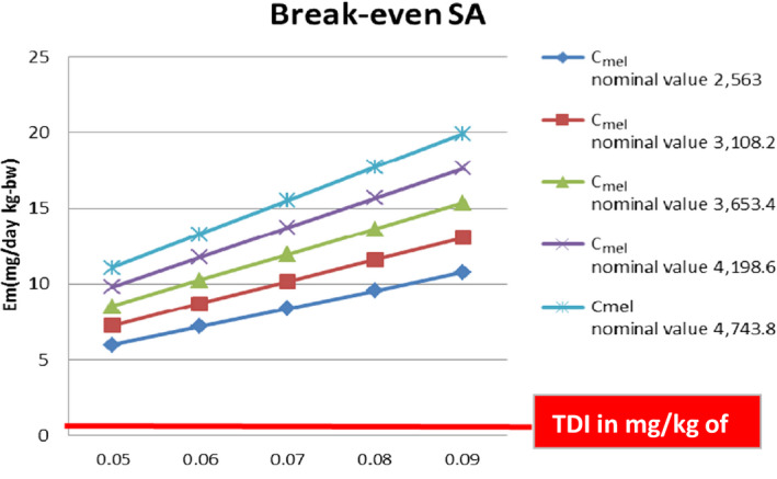
Results of break‐even sensitivity analysis

Example based on the Morris method for sensitivity analysis

Table B.39 presents the input distributions, used for the Morris and Sobol methods. These are based on the outputs of the 2D Monte Carlo simulation, by taking the medians of the uncertainty distributions of the mean and standard deviation of the variability distributions for 1‐year‐old children. These were then converted in parameters for the distributions used in the global sensitivity analysis. As in other examples, uncertainty in the TDI was not considered. For both methods, the distributions were truncated at the 0.1 and 99.9 percentiles to prevent a strong influence of extreme values.

Table B.39.

Distribution of input factors for computation of exposure distribution

Input factor	Description	Unit	Mean	SD	Range	Distribution
C	Concentration of melamine in milk powder	mg/kg	232	627	–	LN(4.34, 1.46)
W	Weight fraction of milk powder in chocolate	–		–	(0.14, 0.30)	U(0.14, 0.30)
Q	Consumption of chocolate	kg/day	0.0142	0.0134		Γ(1.12, 79.1, 0]
Bw	Body weight of children	Kg	11.00	1.53	–	LN(2.39, 0.138]
Tdi	Tolerable Daily Intake	mg/kg/day	0.50	–	Constant	Constant

Results of the Morris method are given in table B40 and figure B22 below. For this linear model, the mean of the elementary effects (μ_i) and the mean of the absolute values of the elementary effects (μ*_i) are the same for all input factors except body weight. All input factors have (almost) linear effects and there are limited interactions among factors (measured by the standard error of the elementary effects – σ_i), as expected from the simplicity of the model structure. The risk ratio r is most sensitive to variations in c and q and least sensitive to variations in bw. The blue and red lines in the Morris graph (Figure B.22) indicate proposed qualitative thresholds where factors’ main influence is in the form of direct effects (below the line) or higher order/interactions (above the line). The red line was proposed originally by Morris (1991) for μ_i and the blue line by Muñoz‐Carpena et al. (2007) and Chu‐Agor et al. (2012)for μ*_i. The results indicate that there are non‐linear effects for all factors.

Figure B.22.

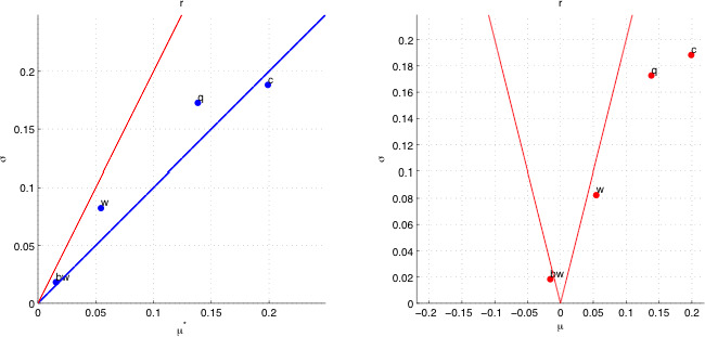
Elementary effects of input factors in the melamine model on the risk ratio r, according to the method of Morris (160 samples). See text for explanation of red and blue lines

Table B.40.

Mean and standard deviation of elementary effects of input factors in the melamine model on the risk ratio r, according to the method of Morris (60 samples)

Input factor	μi*	μi	σi
C	0.20	0.20	0.19
W	0.05	0.05	0.08
Q	0.14	0.14	0.17
Bw	0.02	−0.02	0.02

Example based on Monte Carlo filtering

For the melamine example, a natural threshold value for the risk ratio, set by risk managers or stakeholders would be r = 1 but, since only few realisations of such values were observed, we chose a threshold of r = 0.1. Figure B.23 shows the MCF results for q and c, the two input factors with the greatest influence on the model output variance, as identified by the Sobol method. According to the Smirnov test, c and q distributions are significantly different and the figure demonstrates that the probability density functions (pdfs) of c are more separated than those of q, indicating that a management intervention to reduce the concentration of melamine in chocolate might be more effective than reducing chocolate consumption. The intersection of the two distributions for c is at ~ 100 mg/kg, hence above the median but below the mean of the input distribution. The intersection of the two distributions for q is at 0.009 g/day, somewhat lower than the mean consumption. This implies that an intervention (policy, regulation) to limit values of c and q at the threshold identified (c < 100 mg/kg and q < 0.009 g/day) would result in the reduction of the risk of children being exposed to more than 10% of the TDI. This illustrates the opportunities of this analysis to transfer the results to risk managers. This result must be considered within the ranges specified for these input factors.

Figure B.23.

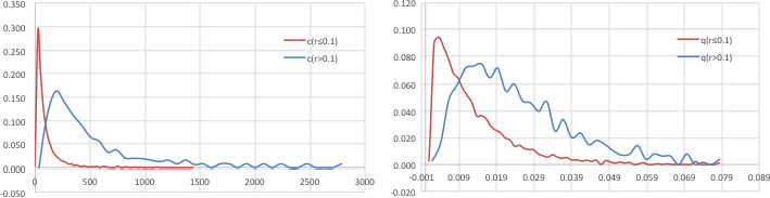
Monte Carlo filtering for melamine example: pdf's of c and q producing favourable (r ≤ 0.1) or unfavourable (r > 0.1) results

Example using Sobol Index

For the melamine example, the variance decomposition is shown in Table B.41. The sum of the first‐order indices is ∑S _i  = 0.74 > 0.6, indicating the model behaves as a mostly additive model for this simple application. Again, the model outputs are most sensitive to variations in c (54% of the total model variance) and to a lesser extent to q (19%). Variations in w and bw hardly affect the model results.

Table B.41.

Variance decomposition of input factors in the melamine model in relation to the risk ratio r, according to the method of Sobol (5,120 samples, M = 512)

Input	First‐order index	Total order index	Interaction index
c	0.54	0.82	0.28
w	0.01	0.03	0.02
q	0.19	0.46	0.27
bw	0.00	0.00	0.00

The Sobol method is based on an efficient Monte Carlo sampling algorithm, exploring the joint parameter space instead of the marginal distributions. Therefore, even though the number of samples is limited, the results can directly be used for uncertainty analysis by reading the Cumulative Density Function (CDF) from the samples of the model Y = f(X1, X2, …, Xk). In the melamine example, the uncertainty in r is graphically represented as in Figure B.24. In this example, the uncertainty should be interpreted as due to variability in the input factors. To include uncertainty in the variability distributions of the input factors, their parameters should be described by probability distributions as in a 2D Monte Carlo simulation. Based on the results of the analysis of variability, parameter uncertainties would only need to be specified for q and c.

Figure B.24.

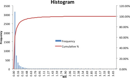
Model output uncertainty pdf for risk ratio r (x‐axis) (N = 5,120 samples)

Example of sensitivity analysis for a percentile of variability

The approach is illustrated by application to the 95th percentile of variability of the risk ratio r. Figure B.25 shows a Sobol–Owen analysis of sensitivity of the estimate of the percentile to the parameters of distributions for variability in the 2D Monte Carlo analysis provided in Annex B.14. It shows very clearly that uncertainty about the parameter σ_logc (standard deviation of log concentration) is the biggest contributor to uncertainty about the 95th percentile of r. Figure B.26 explores the nature of the influence of σ_logc on uncertainty about the 95th percentile of r. It shows that higher values of σ_logc lead to a distribution for which is concentrated on higher values for the 95th percentile of r.

Figure B.25.

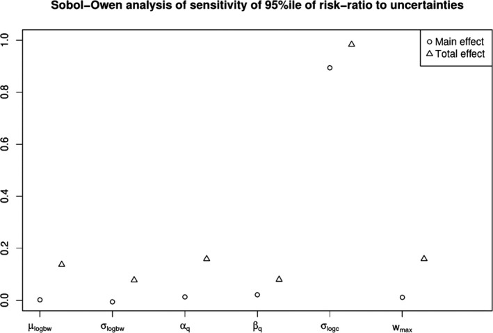
Sobo–Owen analysis of sensitivity of the 95th percentile of the risk‐ratio r to uncertainties about statistical parameters

Figure B.26.

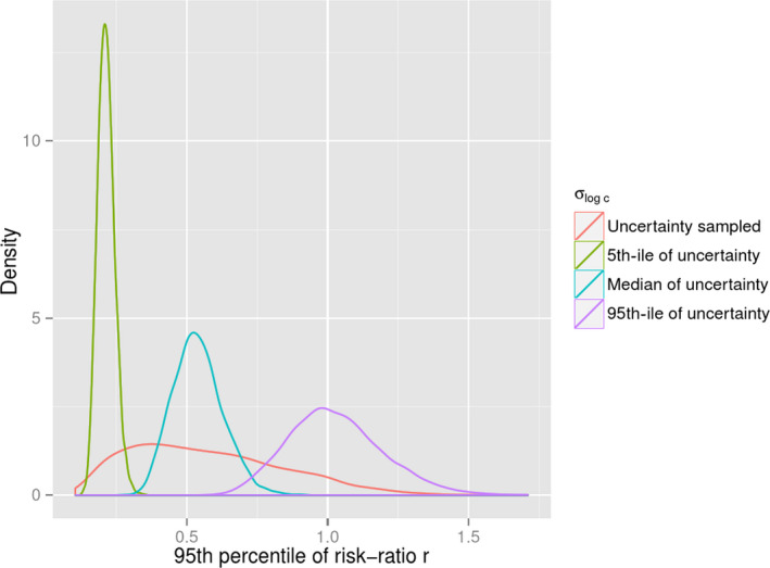
Uncertainty about the 95th percentile of the risk‐ratio r in four scenarios for the parameter σ_logc which is the standard deviation of log concentration. Three scenarios show the consequences of fixing the parameter at different percentiles of uncertainty and the fourth shows the consequence of using the full distribution of uncertainty for the parameter

Sensitivity analysis in the melamine example: general considerations

Irrespective of the method used to perform sensitivity analysis, the ranking of the input factors according to their influence on the output of the model is extremely robust. Melamine concentration and chocolate consumption are the variables largely explaining the variability/uncertainty of the exposure and the risk ratio. In a real assessment this result could be communicated to risk managers and support an informed decision about actions to reduce exposure and risk.

Methodology for full separation of variability and uncertainty in sensitivity analysis is not yet well established. Therefore, it has not been considered in this example. Further research is needed in this direction.

Strengths

1. Provide extremely valuable information for making recommendations to policy makers (e.g. identifying factors on which it is more effective to concentrate resources and actions in order to reduce risk).

2. Allows prioritisation of parameters for uncertainty analysis and/or further research.

3. Some methods are very easy to implement and understand (e.g. nominal range methods).

Weaknesses and possible approaches to reduce them

1. When risk assessment involves many model parameters, sensitivity analysis can be quite computationally intense. Screening of input factors (e.g. using graphical methods or method of Morris) can be used to reduce dimensionality.

2. Some methodologies rely on assumptions related to relationship between inputs and output (e.g. linearity) and among inputs (e.g. independence). When these assumptions do not hold, conclusions of the SA can be misleading; methods that are able to address non linearity and dependency should be preferred in these cases.

3. It is necessary to clarify prior to start the sensitivity analysis which question it is intended to answer, otherwise its value could be limited and not addressing the informative needs.

4. Generally, it is not possible to separate influence of each input on the output in terms of variability and uncertainty of the input separately. Only methods recently developed allow so (Busschaert et al. 2011).

5. The sensitivity analysis has been already occasionally applied in EFSA. Still a regular application (especially when models are used as a basis for the assessment) is not in place. The application of scenario analysis (conditional sensitivity analysis) is more frequent but not a common practice.

6. Training should be provided to staff and experts in order to facilitate the performance of sensitivity analysis. This training should include guidance on preferable methods to be included in different domains/scientific assessment types.

Assessment against evaluation criteria

There is a large variability in the nature and complexity of the methods that can be used to perform a sensitivity analysis. Consequently it was decided to have two tables assessing deterministic (Table B.42) and probabilistic methods (Table B.43) separately against evaluation criteria. The item ‘meaning of output’ was deliberately not filled in since sensitivity analysis complements uncertainty analysis without providing a direct measure of it.

Table B.42.

Assessment of Deterministic methods for sensitivity analysis (when applied well) against evaluation criteria

Criteria	Evidence of current acceptance	Expertise needed to conduct	Time needed	Theoretical basis	Degree/extent of subjectivity	Method of propagation	Treatment of uncertainty and variability	Meaning of output	Transparency and reproducibility	Ease of understanding for non‐specialist
Stronger characteristics	International guidelines or standard scientific method	No specialist knowledge required	Hours	Well established, coherent basis for all aspects	Judgement used only to choose method of analysis	Calculation based on appropriate theory	Different types of uncertainty & variability quantified separately	Range and probability of possible answers	All aspects of process and reasoning fully documented	All aspects fully understandable
	EU level guidelines or widespread in practice	Can be used with guidelines or literature	Days	Most but not all aspects supported by theory	Combination of data and expert judgement	Formal expert judgement	Uncertainty and variability quantified separately	Range and relative possibility of answers	Most aspects of process and reasoning well documented	Outputs and most of process understandable
	National guidelines, or well established in practice or literature	Training course needed	Weeks	Some aspects supported by theory	Expert judgement on defined quantitative scales	Informal expert judgement	Uncertainty and variability distinguished qualitatively	Range of answers but no weighting	Process well documented but limited explanation of reasoning	Outputs and principles of process understandable
	Some publications and/or regulatory practice	Substantial expertise or experience needed	A few months	Limited theoretical basis	Expert judgement on defined ordinal scales	Calculation or matrices without theoretical basis		Quantitative measure of degree of uncertainty	Limited explanation of process and/or basis for conclusions	Outputs understandable but not process
Weaker characteristics	Newly developed	Professional statistician needed	Many months	Pragmatic approach without theoretical basis	Verbal description, no defined scale	No propagation	No distinction between variability and uncertainty	Ordinal scale or narrative description for degree of uncertainty	No explanation of process or basis for conclusions	Process and outputs only understandable for specialists

Table B.43.

Assessment of Probabilistic methods for sensitivity analysis (when applied well) against evaluation criteria

Criteria	Evidence of current acceptance	Expertise needed to conduct	Time needed	Theoretical basis	Degree/extent of subjectivity	Method of propagation	Treatment of uncertainty and variability	Meaning of output	Transparency and reproducibility	Ease of understanding for non‐specialist
Stronger characteristics	International guidelines or standard scientific method	No specialist knowledge required	Hours	Well established, coherent basis for all aspects	Judgement used only to choose method of analysis	Calculation based on appropriate theory	Different types of uncertainty & variability quantified separately	Range and probability of possible answers	All aspects of process and reasoning fully documented	All aspects fully understandable
	EU level guidelines or widespread in practice	Can be used with guidelines or literature	Days	Most but not all aspects supported by theory	Combination of data and expert judgement	Formal expert judgement	Uncertainty and variability quantified separately	Range and relative possibility of answers	Most aspects of process and reasoning well documented	Outputs and most of process understandable
	National guidelines, or well established in practice or literature	Training course needed	Weeks	Some aspects supported by theory	Expert judgement on defined quantitative scales	Informal expert judgement	Uncertainty and variability distinguished qualitatively	Range of answers but no weighting	Process well documented but limited explanation of reasoning	Outputs and principles of process understandable
	Some publications and/or regulatory practice	Substantial expertise or experience needed	A few months	Limited theoretical basis	Expert judgement on defined ordinal scales	Calculation or matrices without theoretical basis		Quantitative measure of degree of uncertainty	Limited explanation of process and/or basis for conclusions	Outputs understandable but not process
Weaker characteristics	Newly developed	Professional statistician needed	Many months	Pragmatic approach without theoretical basis	Verbal description, no defined scale	No propagation	No distinction between variability and uncertainty	Ordinal scale or narrative description for degree of uncertainty	No explanation of process or basis for conclusions	Process and outputs only understandable for specialists

Conclusions

1. Sensitivity analysis can represent a valuable complement of uncertainty analysis in EFSA. It helps assessors in providing risk managers with information about most influential factors on which to focus actions and further research.

2. It has potential for applicability in any area of work in EFSA.

3. Obstacles to application of the method could be technical complexity and the need to involve an experienced statistician in the computation and interpretation of some specific methods. Training should be provided to staff and experts in order to facilitate the performance of sensitivity analysis.

4. It is necessary to clarify prior to start the sensitivity analysis which question it is intended to reply, otherwise its value could be limited and not addressing the informative needs.

References

Augustin J‐C, 2011. Global sensitivity analysis applied to food safety risk assessment. Electronic Journal of Applied Statistical Analysis, 4, 255–264. https://doi.org/10.1285/i20705948v4n2p255

Busschaert P, Geeraerd AH, Uyttendaele M and Van Impe JF, 2011. Sensitivity analysis of a two‐dimensional quantitative microbiological risk assessment: keeping variability and uncertainty separated. Risk Analysis, 31, 1295–1307.

Chu‐Agor ML, Munoz‐Carpena R, Kiker GA, Aiello‐Lammens ME, Akcakaya HR, Convertino M and Linkov L, 2012. Simulating the fate of Florida Snowy Plovers with sea‐level rise: Exploring research and management priorities with a global uncertainty and sensitivity analysis perspective. Ecological Modelling, 224, 33–47.

Cukier RI, Fortuin CM, Shuler KE, Petschek AG, Schaibly JH and Chern J, 1973. Study of the sensitivity of coupled reaction systems to uncertainties in rate coefficients. I Theory. The Journal of Chemical Physics, 59, 3873–3878.

Cullen AC and Frey HC, 1999. Probabilistic techniques in exposure assessment. Plenum Press. New York.

ECHA, 2012. Guidance on information requirements and chemical safety assessment. Chapter R19: Uncertainty analysis. ECHA‐12‐G‐25‐EN. Available online: http://echa.europa.eu/documents/10162/13632/information_requirements_r19_en.pdf

EFSA PPR Panel (Panel on Plant Protection Products and their Residues), 2012. Guidance on the Use of Probabilistic Methodology for Modelling Dietary Exposure to Pesticide Residues. EFSA Journal 2012;10(10):2839. Available online: www.efsa.europa.eu/efsajournal

EFSA AHAQ Panel (EFSA AHAW Panel on Animal Health and Welfare), 2007. Framework for the AHAW Risk Assessments. EFSA Journal 2007; 550, 1–46.

EFSA (European Food Safety Authority), 2014. Analysis of the baseline survey on the prevalence of Listeria monocytogenes in certain ready‐to‐eat foods in the EU, 2010–2011. Part B: analysis of factors related to prevalence and exploring compliance. EFSA Journal 2014;12(8):3810, 73 pp. Available online: www.efsa.europa.eu/efsajournal

Ekstrom P, 2005. EIKOS a simulation toolbox for sensitivity analysis. Degree project 20p. Uppsala University. Faculty of Science and Technology. The UTH_Unit.

Frey HC and Patil SR, 2002. Identification and review of sensitivity analysis methods, Risk Analysis, 22, 553–78.

Homma T and Saltelli A, 1996. Importance measures in global sensitivity analysis of nonlinear models. Reliability Engineering and System Safety, 52, 1–17.

Khare YP, Muñoz‐Carpena R, Rooney RW and Martinez CJ. A multi‐criteria trajectory‐based parameter sampling strategy for the screening method of elementary effects. Environmental Modelling & Software, 64, 230–239.

Morris MD, 1991. Factorial sampling plans for preliminary computational experiments. Technometrics, 33, 161–174.

Muñoz‐Carpena R, Zajac Z and Kuo YM, 2007. Evaluation of water quality models through global sensitivity and uncertainty analyses techniques: application to the vegetative filter strip model VFSMOD‐W. Trans ASABE, 50, 1719–1732.

Pannell DJ, 1997. Sensitivity analysis of normative economic models: Theoretical framework and practical strategies, Agricultural Economics, 16, 139–152.

Patil SR and Fray HC, 2004. Comparison of sensitivity analysis methods based on applications to a food safety risk assessment model. Risk Analysis, 24, 573–585.

US NRC (US Nuclear Regulatory Commission), 2013. Risk assessment in regulation. Available online: http://www.nrc.gov/about-nrc/regulatory/risk-informed.html

Saltelli A, Tarantola S and Chan KPS, 1999. A quantitative model‐independent method for global sensitivity analysis of model output. Technometrics, 41, 39–56.

Saltelli A, Tarantole S, Campolongo F and Ratto M, 2004. Sensitivity analysis in practice. A guide to assessing scientific models. Wiley‐Interscience.

Saltelli A, Ratto M, Tarantola S and Campolongo F, 2005. Sensitivity analysis for chemical models. Chemical Reviews, 105, 2811–2828.

Saltelli A, Ratto M, Andres T, Campolongo F, Cariboni J, Gatelli D, Saisana M and Tarantola S, 2008. Global sensitivity analysis: the primer. Wiley‐Interscience.

Sobol IM, 1990. Sensitivity estimates for nonlinear mathematical models. Translated as I M Sobol 1993 Sensitivity analysis for non‐linear mathematical models Math Modeling Comput Experiment, 1, 407–414. 1990; 2, 112–118.

B.18. Probability calculations for logic models

Purpose, origin and principal features

A logic model is a way to represent the structure of a logical deduction about a yes/no conclusion based on the answers to a series of yes/no questions. The context needs to be such that the conclusion is certain if there is no uncertainty about the answers to the questions. Situations where there would be residual uncertainty about the conclusion are best addressed by another method: Bayesian graphical modelling (see Section 11.5.2).

Logic models are based fundamentally on Boolean algebra (Boole, 1854) which is the generally accepted mathematical formalism for describing logical relations and which underlies digital electronics and computers. The diagrams for visualising logic models shown in the example are very similar in spirit to standard digital logic gate diagrams used in electronics.

The simplest logic models are the primitive ‘and’ and ‘or’ models. In the ‘and’ model, the conclusion is ‘yes’ if and only if the answer to each question is ‘yes’. In the ‘or’ model, the conclusion is ‘yes’ unless the answer to each question is ‘no’. By combining the primitive models hierarchically in a tree where the root of the tree is the conclusion and the leaves are the individual questions, any logical deduction can be modelled. The structure of the reasoning is made explicit by showing the model as a diagram.

A logic model provides a transparent basis for subsequent probability calculations leading to quantifying combined uncertainty about the conclusion based on probabilities expressing uncertainty about the answers to the questions. Calculations required to compute the probability that the conclusion is ‘yes’ are standard elementary probability calculations: the diagram simply organises and supports the calculations. The probabilities for the answers to the questions may be based on statistical analysis of data (see Section 11.2) or may derive directly from expert knowledge elicitation (see Section 11.3). Logic models used in this way have a similar function to network models used in engineering reliability assessment (Billinton and Allan, 1992).

Calculating the probability for the conclusion from probabilities for the questions

If uncertainty is expressed for each question by specifying the probability of ‘yes’, the probability that the conclusion is ‘yes’ can be calculated using the mathematics of probability. For the ‘and’ model, the probability of ‘yes’ for the conclusion is obtained by multiplying the probabilities for the individual questions. Denoting the probability of ‘yes’ for the conclusion by p and the probabilities of ‘yes’ for n questions by p₁, …, p_n:

$$\mathrm{p}={\mathrm{p}}_1\times \dots \times {\mathrm{p}}_{\mathrm{n}}$$

In order to describe the calculation for the ‘or’ model, first note that for any ‘yes’/’no’ outcome, the probabilities for the two outcomes must sum to 100%. The probability of ‘no’ for the conclusion is obtained by multiplying the probability of ‘no’ for each of the questions. Therefore, for the ‘or’ model:

$$\mathrm{p}=1-(1-{\mathrm{p}}_1)\times \dots \times (1-{\mathrm{p}}_{\mathrm{n}})$$

For a logic model represented as a tree where the leaves correspond to the questions, the calculation works by first finding a group of leaves connected in a primitive ‘and’ model or ‘or’ model. Each of those leaves has an associated probability of ‘yes’. The calculation described above is then carried out for the primitive model and the group of leaves is replaced by a single new leaf which has the probability of ‘yes’ resulting from the calculation. By repeating the process until there is left only a single leaf corresponding to the conclusion, the probability of ‘yes’ for the conclusion is calculated.

Calculations using approximate probabilities

The description above assumes that the probability of ‘yes’ for each question has been specified precisely. If any of the probabilities has been specified approximately as a range (see Section 5.11), interval analysis (Section 12, Annex B.7) can be used to compute the resulting approximate probability relating to the conclusion. Any precise probability specified should first be converted to an equivalent approximate probability for which both lower and upper bounds coincide with the probability specified. For both primitive models, the lower bound for the probability for the conclusion is obtained by applying the calculation described above to the lower bounds for the individual probabilities and the upper bound obtained by applying the calculation to the individual upper bounds. For general models, the calculation of approximate probabilities for primitive models can be propagated through the tree to the root, as described above for precise probabilities, in order to arrive at an approximate probability for the conclusion.

Using negations

In principle, it is possible to express any logical deduction as a tree using only ‘and’ and ‘or’ combinations. To do so, it may be necessary to negate the framing of some questions, i.e. to reframe a question to reverse the meaning of ‘yes’ and ‘no’ as answers. An alternative, which may feel more natural in some situations, is to incorporate ‘not’ operations in the tree. A ‘not’ operation sits between a question or intermediate deduction and the primitive model to which it contributes information. It negates the answer to the question or intermediate deduction. The corresponding calculation for a precise probability is to replace the probability by its complement, i.e. to subtract the probability from 100%. For an approximate probability, the upper and lower bounds are both subtracted from 100% and in doing so the lower bound becomes the new upper bound and vice versa.

Dependence

If there is dependence between uncertainties which feed into different primitive models in the original tree, it is still possible to do calculations. However, greater expertise is needed in carrying out probability calculations and it would be sensible to seek advice.

It is more straightforward to address dependence between uncertainties about questions which feed into the same primitive model in the original tree. The dependent questions need to be isolated into a separate primitive model which then contributes to the original primitive model (this is always possible). Then there are two approaches to establishing the probability of ‘yes’ for the new separate primitive model: either specify directly the probability of ‘yes’ for the new primitive model or calculate it using specified conditional probabilities. If taking the latter approach for an ‘and’ model, the probability of ‘yes’ for the new model is obtained by first specifying the probability of ‘yes’ for one question and then, in sequence for each of the other dependent questions, multiplying by the conditional probability for that question of ‘yes’ given that the answer to each preceding question is ‘yes’. If the new model is an ‘or’ model, first reformulate it as an ‘and’ model followed by a ‘not’ and then apply the conditional probability approach to the ‘and’ model.

Applicability in areas relevant for EFSA

Applicable to all areas of EFSA's work but restricted to assessments or parts of assessments where a yes/no conclusion can be represented as logical deductions from answers to a series of yes/no questions.

Potential contribution to major steps of uncertainty analysis

Steps in uncertainty analysis	Potential contribution of this approach
Identifying uncertainties	Not applicable
Characterising uncertainties	Not applicable
Combining uncertainties	Yes (for yes/no questions)
Prioritising uncertainties	Not applicable

Example

For illustrative purposes, consider a situation where it is judged that a hazard to humans exists for a particular chemical if and only if it produces one of two possible toxic metabolites in humans and the individual exposed belongs to a particular genetic subpopulation. This reasoning process can be expressed as a diagram involving yes/no questions:

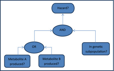
Note that the diagram and calculations below are specific to the situation where there are two toxic metabolites and would need to be altered if there was a different or uncertain number of toxic metabolites.

Suppose also that the following hypothetical judgements are made about uncertainties about the answer to the three questions: they are judged to be independent, the probability that metabolite A is produced is 30%, the probability that metabolite B is produced is 20% and the probability that an individual belongs to the genetic subgroup is 5%. The calculation of the probability of hazard proceeds hierarchically. First, the ‘or’ model is calculated, replacing the ‘OR’ box by an intermediate conclusion having probability $1-(1-.3)(1-.2)=44$%. Then the ‘and’ model is calculated to conclude that the probability of hazard is $.44\times .05=2.2$%.

As an example of the use of ‘not’ operators, the following diagram represents the same logical model and leads to the same probability of hazard:

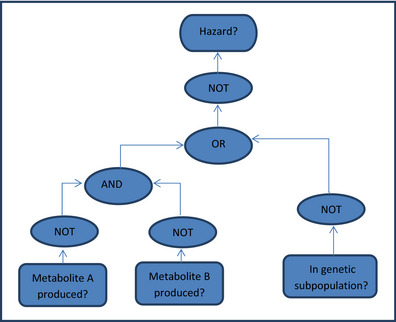
As an example of how to address dependence, suppose that judgements of uncertainty about the production of the two metabolites are considered to be dependent. As discussed above, there are two possible approaches to addressing the dependence, based on the second diagram. The first approach is to directly specify the probability that neither metabolite is produced. The second approach would be to calculate the probability that neither metabolite is produced by (i) specifying the probability that metabolite A is not produced; (ii) specifying the conditional probability, given that A is not produced, that metabolite B is not produced; (iii) multiplying the numbers from steps (i) and (ii). Either way, the resulting probability, that neither metabolite is produced, would then replace the ‘AND’ and the branches and leaves from the ‘AND’.

Strengths

1. Provides diagrams to represent the structure of logical deduction of a yes/no conclusion from a series of yes/no questions.

2. Provides a probability for the conclusion calculated from probabilities for the answers to the questions.

3. Relatively easy to apply if some or all probabilities are approximate.

4. It is possible to take account of dependence between uncertainties about answers to questions.

Weaknesses and possible approaches to reduce them

1. Only applies to yes/no conclusions deduced from answers to yes/no questions.

2. Only applies to conclusions which would not be uncertain if there was no uncertainty about the answers to the underlying questions. In other situations, Bayesian graphical modelling (Section 11.5.2) should be used

3. Some forms of dependence require specialist expertise.

Assessment against evaluation criteria

This method is assessed against the criteria in Table B.44. In evaluating time needed, time needed to conduct EKE or analyse data is not included.

Table B.44.

Assessment of calculations using logic models (when used well) against evaluation criteria

Criteria	Evidence of current acceptance	Expertise needed to conduct	Time needed	Theoretical basis	Degree/extent of subjectivity	Method of propagation	Treatment of uncertainty and variability	Meaning of output	Transparency and reproducibility	Ease of understanding for non‐specialist
Stronger characteristics	International guidelines or standard scientific method	No specialist knowledge required	Hours	Well established, coherent basis for all aspects	Judgement used only to choose method of analysis	Calculation based on appropriate theory	Different types of uncertainty & variability quantified separately	Range and probability of possible answers	All aspects of process and reasoning fully documented	All aspects fully understandable
	EU level guidelines or widespread in practice	Can be used with guidelines or literature	Days	Most but not all aspects supported by theory	Combination of data and expert judgement	Formal expert judgement	Uncertainty and variability quantified separately	Range and relative possibility of answers	Most aspects of process and reasoning well documented	Outputs and most of process understandable
	National guidelines, or well established in practice or literature	Training course needed	Weeks	Some aspects supported by theory	Expert judgement on defined quantitative scales	Informal expert judgement	Uncertainty and variability distinguished qualitatively	Range of answers but no weighting	Process well documented but limited explanation of reasoning	Outputs and principles of process understandable
	Some publications and/or regulatory practice	Substantial expertise or experience needed	A few months	Limited theoretical basis	Expert judgement on defined ordinal scales	Calculation or matrices without theoretical basis		Quantitative measure of degree of uncertainty	Limited explanation of process and/or basis for conclusions	Outputs understandable but not process
Weaker characteristics	Newly developed	Professional statistician needed	Many months	Pragmatic approach without theoretical basis	Verbal description, no defined scale	No propagation	No distinction between variability and uncertainty	Ordinal scale or narrative description for degree of uncertainty	No explanation of process or basis for conclusions	Process and outputs only understandable for specialists

Conclusions

1. This is potentially an important tool for EFSA as it provides a way to structure logical arguments involving yes/no conclusions and to calculate the combined uncertainty about a conclusion based on uncertainty about underlying yes/no questions expressed using probability.

References

Billinton R and Allan RN, 1992. Reliability Evaluation of Engineering Systems: Concepts and Techniques. Springer, USA.

Boole G, 1854. An Investigation of the Laws of Thought on which are Founded the Mathematical Theories of Logic and Probabilities. Walton and Maberley.

B.19. Structured tools for evidence appraisal

Purpose, origin and principal features

Appraisal of the risk of bias in the individual studies used as evidence in an assessment is a standard step when using data from literature (Higgins and Green, 2011, updated 2017). Risk of bias can affect a study in terms of limitations in the internal and/or external validity. They both imply an uncertainty: the first around the extent to which the findings of the study accurately estimate its own target outcome, the second around the extent to which these findings can be extrapolated to the outcome of an assessment. Examples of threats to internal validity are confounding factors in observational studies and the use of unreliable measures of exposure. Risk of bias is different from quality of a study in the sense that perfectly designed studies can still be affected by risk of bias.

Several structured frameworks have been developed for assessing risk of bias in an individual study, sometimes referred to as Critical Appraisal Tools (CATs), that take the form of check lists and are tailored by study design (e.g. randomised controlled trials). These include a standardised list of items representing potential sources of uncertainty (e.g. lack of randomisation in a randomised controlled trial) that need to be evaluated in the light of the potential bias they could have introduced in the results. Originally developed in the context of clinical intervention, their use has rapidly spread to other research questions and study design. Threats to internal validity are generally the only source of uncertainty appraised at the level of an individual study. Other important sources such as external validity and random error (i.e. sampling uncertainty) are normally considered when integrating the evidence (e.g. in a meta‐analysis) and appraising the certainty in the whole body of evidence.

Frameworks have been established also to assess the confidence or certainty in the whole body of evidence (i.e. the set of studies used for the assessment). They generally refer to a set of criteria known as Bradford‐Hill criteria (Bradford‐Hill 1965) that were established to assess whether a causal relationship between a potential harm and a health effect can be concluded on the basis of the available evidence. Original Bradford‐Hill criteria include: strength/size of the effect; consistency of the findings or reproducibility; specificity of the association (no other potential source of the effect are identified); temporality (effect appears after the potential cause); biological gradient or dose response (monotonic relationship is expected either increasing or decreasing); plausibility or biological relevance; coherence among results from various sources of evidence; availability of experimental evidence (considered the most credible source of evidence to establish causation); analogy (consideration of effect of similar factors). Over the years, these criteria has been modified and adapted (Adami et al. 2011) and recently used to develop approaches to evaluate the confidence or certainty in a whole body of evidence when used to support conclusion on causality (GRADE and modified GRADE approaches, see Table B.46 for references).

Table B.46.

Approaches to evaluate the certainty in a body of evidence

Approaches to evaluate overall certainty in the body of evidence	Nature of the approach	Institution	Link/reference
Grading of Recommendations Assessment, Development and Evaluation (short GRADE)	Qualitative	GRADE working group	http://www.gradeworkinggroup.org/
Office of Health Assessment and Translation (OHAT) ‐ Approach for Systematic Review and Evidence Integration	Qualitative	National Toxicology Programme (NTP)	https://ntp.niehs.nih.gov/ntp/ohat/pubs/handbookjan2015_508.pdf
Navigation Guide	Qualitative	University of California San Francisco – Programme on reproductive health and environment	https://prhe.ucsf.edu/navigation-guide
Systematic Review Centre for Laboratory animal Experimentation (in short SYRCLE1)	Qualitative	SYRCLE SR centre	https://www.radboudumc.nl/en/research/technology-centers/animal-research-facility/systematic-review-center-for-laboratory-animal-experimentation

Bias‐adjusted meta‐analysis may be an option to account quantitatively for risk of internal and external bias when integrating evidence systematically retrieved in the literature (e.g. Turner et al., 2009).

Tools to appraise the risk of bias in individual studies tailored to various different study designs are listed in Table B.45, while approaches to evaluate the certainty in the whole body of evidence are listed in Table B.46.

Table B.45.

Tools and methods to evaluate the risk of bias in an individual study

Tool to assess risk of bias at the level of each individual study	Study design/setting in which the tools are applicable	Institution	Link/reference
Office of Health Assessment and Translation (OHAT) RoB Tool	Experimental animal studies, human RCT, human observational	National Toxicology Programme (NTP)	https://ntp.niehs.nih.gov/ntp/ohat/pubs/riskofbiastool_508.pdf
Rob2.0	Risk of bias in randomized trials	Cochrane collaboration	https://sites.google.com/site/riskofbiastool/welcome/rob-2-0-tool
Robins‐I	Risk of Bias in non‐randomized studies ‐ of interventions	Cochrane collaboration	https://sites.google.com/site/riskofbiastool/welcome/home
RoB Diagnostic Test Accuracy	Risk of bias in diagnostic test accuracy	Cochrane Canada	http://training.cochrane.org/resource/primer-cochrane-diagnostic-test-accuracy-reviews
QUADAS‐2	Risk of bias in diagnostic test accuracy	QUADAS‐2 Group
SYRCLE RoB Tool	Experimental animal study	SYRCLE at Central Animal Laboratory
EFSA SR CAT	Risk of bias and imprecision in randomised trials	EFSA	http://onlinelibrary.wiley.com/doi/10.2903/sp.efsa.2015.EN-836/epdf
EFSA SR CAT	Appraisal of Systematic Review process	EFSA	http://onlinelibrary.wiley.com/doi/10.2903/sp.efsa.2015.EN-836/epdf
EFSA ELS CAT	Appraisal of the Extensive Literature Review process	EFSA	http://onlinelibrary.wiley.com/doi/10.2903/sp.efsa.2015.EN-836/epdf
Tool to assess Risk of Bias in cohort studies	Risk of bias in cohort studies	CLARITY Group	https://www.evidencepartners.com/resources/methodological-resources/
Tool to assess Risk of Bias in case control studies	Risk of bias in case control studies	CLARITY Group	https://www.evidencepartners.com/resources/methodological-resources/
Tool to assess Risk of Bias in randomised controlled trials	Risk of bias in RCT	CLARITY Group	https://www.evidencepartners.com/resources/methodological-resources/
Tool to assess Risk of Bias in case control studies	Risk of bias in case control studies	CLARITY Group	https://www.evidencepartners.com/resources/methodological-resources/

Applicability in areas relevant for EFSA

Applicable to all areas of EFSA's work but restricted to assessments or parts of assessments where studies retrieved from the literature are used. It is applicable as well as to submitted studies for regulated products.

Potential contribution to major elements of uncertainty analysis

Elements in uncertainty analysis	Potential contribution of this approach
Identifying uncertainties	Yes
Characterising uncertainties	Yes
Combining uncertainties	Yes
Prioritising uncertainties	Not applicable

Melamine example

Not done.

Strengths

1. Provide a structured approach for consistent identification, evaluation and combination of uncertainties in multiple studies of the same type, or different studies comprising a body of evidence.

2. Facilitate the process of uncertainty identification when uncertainty in the evidence is the main objective.

3. Make the process of uncertainty identification and evaluation transparent and repeatable.

Weaknesses and possible approaches to reduce them

1. Do not express the impact of uncertainties in terms of how different the assessment conclusion could be and how likely that is.

2. Specialist advice (which is available internally in EFSA) may be needed for choosing the appropriate appraisal tool and framework and to adapt them to the domain at hand as appropriate. Training and/or specialist support may be needed to properly apply the tools.

Assessment against evaluation criteria

The use of structured approaches for evidence appraisal is assessed against the criteria in Table B.47.

Table B.47.

Assessment of structured approaches for evidence appraisal (when used well) against evaluation criteria

Criteria	Evidence of current acceptance	Expertise needed to conduct	Time needed	Theoretical basis	Degree/extent of subjectivity	Method of propagation	Treatment of uncertainty and variability	Meaning of output	Transparency and reproducibility	Ease of understanding for non‐specialist
Stronger characteristics	International guidelines or standard scientific method	No specialist knowledge required	Hours	Well established, coherent basis for all aspects	Judgement used only to choose method of analysis	Calculation based on appropriate theory	Different types of uncertainty & variability quantified separately	Range and probability of possible answers	All aspects of process and reasoning fully documented	All aspects fully understandable
	EU level guidelines or widespread in practice	Can be used with guidelines or literature	Days	Most but not all aspects supported by theory	Combination of data and expert judgement	Formal expert judgement	Uncertainty and variability quantified separately	Range and relative possibility of answers	Most aspects of process and reasoning well documented	Outputs and most of process understandable
	National guidelines, or well established in practice or literature	Training course needed	Weeks	Some aspects supported by theory	Expert judgement on defined quantitative scales	Informal expert judgement	Uncertainty and variability distinguished qualitatively	Range of answers but no weighting	Process well documented but limited explanation of reasoning	Outputs and principles of process understandable
	Some publications and/or regulatory practice	Substantial expertise or experience needed	A few months	Limited theoretical basis	Expert judgement on defined ordinal scales	Calculation or matrices without theoretical basis		Quantitative measure of degree of uncertainty	Limited explanation of process and/or basis for conclusions	Outputs understandable but not process
Weaker characteristics	Newly developed	Professional statistician needed	Many months	Pragmatic approach without theoretical basis	Verbal description, no defined scale	No propagation	No distinction between variability and uncertainty	Ordinal scale or narrative description for degree of uncertainty	No explanation of process or basis for conclusions	Process and outputs only understandable for specialists

Conclusions

Structured approaches for appraising the evidence are valuable methods that should be used in EFSA when assessments include evidence retrieved from the literature and when evaluating studies submitted for regulated products. Several critical appraisal tools are available and there is a need to choose the one that is more appropriate to the study design and adapt it where needed to the specific topic and domain. These approaches enhance consistency and transparency in the evaluation of the risk of bias and other types of uncertainties across a body of evidence. However, they need to be used in conjunction with other methods in the guidance to express the impact of the identified uncertainties on assessment conclusions.

References

Adami HO, Berry SC, Breckenridge CB, Smith LL, Swenberg JA, Trichopoulos D, Weiss NS and Pastoor TP, 2011. Toxicology and epidemiology: improving the science with a framework for combining toxicological and epidemiological evidence to establish causal inference. Toxicolcal Science, 122, 223–234. https://doi.org/10.1093/toxsci/kfr113. Epub 2011 May 10.

Bradford HA, 1965. The Environment and disease: association or causation? Proceedings of the Royal Society of Medicine, 58, 295–300.

GRADE working group, 2013. Handbook for grading the quality of evidence and the strength of recommendations using the GRADE approach. Updated October 2013. In: Schünemann H, Brożek J, Guyatt G and Oxman A (eds.). Available online: http://gdt.guidelinedevelopment.org/app/handbook/handbook.html

Higgins JPT, Green S (eds.), 2011. Cochrane Handbook for Systematic Reviews of Interventions Version 5.1.0 [updated March 2011]. The Cochrane Collaboration, 2011. Available online: http://handbook.cochrane.org

Annex C – Further details for the melamine case study

C.1. Deterministic quantitative model

The basic risk assessment model for the case study includes two calculation steps, to calculate first exposure (e):

$$\mathrm{e}=\frac{\mathrm{c}\times \mathrm{w}\times \mathrm{q}}{\text{bw}}$$

and then the risk ratio (r): r = e/TDI. The quantities involved in these calculations are:

c	Concentration of melamine in milk powder	(mg/kg)	Input variable (distribution uncertain)
w	Weight fraction of milk powder in chocolate	(–)	Input variable (distribution uncertain)
q	Consumption of chocolate	(kg/day)	Input variable (distribution uncertain)
bw	Body weight of children	(kg)	Input variable (distribution uncertain)
TDI	Tolerable Daily Intake	(mg/kg per day)	Specified value (but there is uncertainty about whether it is the correct value)
e	Exposure	(mg/kg per day)	Output variable (distribution uncertain)
r	Risk ratio	(–)	Output variable (distribution uncertain)

Two versions of the example are considered: uncertainty about the highest exposure occurring (worst‐case) and uncertainty about variability of exposure. For the first version, the issue of variability has been removed by considering the worst case so that there is only uncertainty to be addressed. For the second, both variability and uncertainty need to be addressed.

In the interval analysis example (Annex B.7), the worst‐case assessment is considered for all children before considering subgroups to address dependence between body weight and consumption. In the other quantitative method examples, attention is restricted to children aged from 1 up to 2 years. An advantage of doing so is that very simple statistical models can be used to illustrate the statistical methods of statistical inference.

C.2. Worst‐case assessment (uncertainty but no variability)

The worst‐case value for the risk‐ratio is r_max = e_max/TDI where

$${\mathrm{e}}_{\max }=\frac{{\mathrm{c}}_{\max }\times {\mathrm{w}}_{\max }\times {\mathrm{q}}_{\max }}{{\text{bw}}_{\min }}$$

The new quantities involved in these calculations are:

rmax	Highest occurring value for the risk ratio	(–)	Output parameter (value uncertain)
emax	Highest occurring exposure	(mg/kg per day)	Output parameter (value uncertain)
cmax	Highest occurring concentration of melamine in milk powder	(mg/kg)	Input parameter (value uncertain)
wmax	Highest occurring weight fraction of milk powder in chocolate	(–)	Input parameter (value uncertain)
qmax	Highest occurring consumption of chocolate	(kg/day)	Input parameter (value uncertain)
bwmin	Lowest occurring body weight of children	(kg)	Input parameter (value uncertain)

C.3. Uncertainty about variability of exposure

Attention was further restricted to children consuming contaminated chocolate from China.

For each of the input variables, a parametric family of distributions was chosen with which to model the variability. In the cases of q and bw, the choice of distribution family was informed by analysis of the data. For c and w, the choices were pragmatic ones made for illustrative purposes. Each of the parameters introduced in this table is uncertain and uncertainty about the values of the parameters is the way in which we address uncertainty about the variability for each variable. Details are given in the following table:

Variable	Distribution family	Parameters (statistical)	Meaning of parameters
c	Log‐normal distribution (base 10)	μlogc and σlogc	Mean and standard deviation of log‐concentration
w	Uniform distribution	aw and bw	Lower and upper limit for weight‐fraction
q	Gamma distribution	αq and βq	Shape and rate parameters for gamma distribution for q
bw	Log‐normal distribution (base 10)	μlogbw and σlogbw	Mean and standard deviation of log‐body weight

C.4. Data used for modelling variability of body weight and consumption

For q and bw, consumption survey data were available, for 1‐year‐old children, from EFSA ( http://www.efsa.europa.eu/en/datexfoodcdb/datexfooddb.htm) and which existed in 2008. The data derive from five surveys carried out in Finland, Germany, Italy, Poland and Spain. They record daily consumption (weight) of ‘Chocolate (cocoa) products’. Restricting to records with positive consumption, they provide 362 values of q for 171 children and the value of bw for each child.

Standard goodness‐of‐fit tests show that the log‐normal family of distributions is a better fit to the bw data than either the normal or gamma families. The log‐normal fit is visually excellent although it does formally fail the tests. For q, the gamma family fits better than normal, log‐normal or Weibull and the visual fit is again good.

The plot below shows the relationship between q and bw for the data used. The correlation is statistically significant, with or without logarithmic transformation of variables, but nevertheless small: 0.13 for the raw data and 0.24 after logarithmic transformation of both variables. Since the examples are intended primarily to illustrate the methods and not to be a complete assessment of uncertainty for the melamine case study and incorporating dependence into the examples in Annex B would involve considerable extra complexity, variability of b and q is treated as independent in the examples of probability bounds analysis and Monte Carlo.

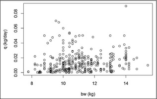
Suggested citation: EFSA Scientific Committee , Benford D, Halldorsson T, Jeger MJ, Knutsen HK, More S, Naegeli H, Noteborn H, Ockleford C, Ricci A, Rychen G, Schlatter JR, Silano V, Solecki R, Turck D, Younes M, Craig P, Hart A, Von Goetz N, Koutsoumanis K, Mortensen A, Ossendorp B, Germini A, Martino L, Merten C, Mosbach‐Schulz O, Smith A and Hardy A, 2018. Scientific Opinion on the principles and methods behind EFSA's Guidance on Uncertainty Analysis in Scientific Assessment. EFSA Journal 2018;16(1):5122, 235 pp. 10.2903/j.efsa.2018.5122

References

- Albert I, Espié E and de Valk H, 2011. A Bayesian evidence synthesis for estimating campylobacteriosis prevalence. Risk Analysis 31, 1141–1155. [DOI] [PubMed] [Google Scholar]
- ANSES , 2016. Avis de l'Anses. Rapport d'expertise collective. Prise en compte de l'incertitude en évaluation des risques: revue de la literature et recommandations pour l'Anses. Available online: https://www.anses.fr/en/system/files/AUTRE2015SA0090Ra.pdf
- ARASP (Center for Advancing Risk Assessment Science and Policy), 2015. Workshop on Evaluating and Expressing Uncertainty in Hazard Characterization, Society of Toxicology (SOT) Annual Meeting. Available online: blog.americanchemistry.com/2015/04/what‐you‐may‐have‐missed‐at‐sot‐how‐show‐and‐tell‐can‐lead‐to‐a‐greater‐understanding‐of‐chemical‐assessment‐results
- Arunraj NS, Mandal S and Maiti J, 2013. Modeling uncertainty in risk assessment: an integrated approach with fuzzy set theory and Monte Carlo simulation. Accident Analysis and Prevention, 55, 242–255. [DOI] [PubMed] [Google Scholar]
- Bailer AJ, Noble RB and Wheeler MW, 2005. Model uncertainty and risk estimation for quantal responses. Risk Analysis, 25, 291–299. [DOI] [PubMed] [Google Scholar]
- BfR (Bundesinstitut für Risikobewertung), 2013. Risk Perception and Crisis Communication – How to Deal with Uncertainty. Presentation by Dr. Suzan Fiack, Symposium “How to overcome a life‐threatening crisis in the food chain”, Berlin. Available online: http://www.bfr.bund.de/cm/343/risk-perception-and-crisis-communication-how-to-deal-with-uncertainty.pdf
- BfR (Bundesinstitut für Risikobewertung), 2015. Guidance document on uncertainty analysis in exposure assessment Recommendation of the Committee for Exposure Assessment and Standardisation of the Federal Institute for Risk Assessment. Available online: http://www.bfr.bund.de/cm/350/guidelines-on-uncertainty-analysis-in-exposure-assessments.pdf
- Bouwknegt M and Havelaar AH, 2015. Uncertainty analysis using the NUSAP approach: a case study on the EFoNAO tool. EFSA supporting publication 2015:EN‐663, 20 pp. [Google Scholar]
- Box GEP, 1976. “Science and Statistics” (PDF). Journal of the American Statistical Association, 71, 791–799. 10.1080/01621459.1976.10480949 [DOI] [Google Scholar]
- Budescu DV, Por H‐H and Broomell SB, 2012. Effective communication of uncertainty in the IPCC reports. Climatic Change, 113, 181–200. [Google Scholar]
- Budescu DV, Por H‐H, Broomell SB and Smithson M, 2014. The interpretation of IPCC probabilistic statements around the world. Nature Climate Change, 4, 508–512. [Google Scholar]
- Codex , 2016. Codex Alimentarius Commission. Procedural Manual. 25th Edition.
- Cooke RM, 2015. Messaging climate change uncertainty. Nature Climate Change 5, 8–10. [Google Scholar]
- Dubois D and Prade H, 1988. Possibility Theory: An Approach to Computerized Processing of Uncertainty. Springer, USA. [Google Scholar]
- ECHA (European Chemicals Agency), 2008. Guidance on information requirements and chemical safety assessment. Chapter R.19: Uncertainty analysis. European Chemicals Agency (ECHA).
- ECHA (European Chemicals Agency), 2012. Chapter R.19 of the “Guidance on Information Requirements and Chemical Safety Assessment”. Available online: http://echa.europa.eu/guidance-documents/guidance-on-information-requirements-and-chemical-safety-assessment