Detecting stable individual differences in the functional organization of the human basal ganglia

Abstract

Moving from group level to individual level functional parcellation maps is a critical step for developing a rich understanding of the links between individual variation in functional network architecture and cognitive and clinical phenotypes. Still, the identification of functional units in the brain based on intrinsic functional connectivity and its dynamic variations between and within subjects remains challenging. Recently, the bootstrap analysis of stable clusters (BASC) framework was developed to quantify the stability of functional brain networks both across and within subjects. This multi-level approach utilizes bootstrap resampling for both individual and group-level clustering to delineate functional units based on their consistency across and within subjects, while providing a measure of their stability. Here, we optimized the BASC framework for functional parcellation of the basal ganglia by investigating a variety of clustering algorithms and similarity measures. Reproducibility and test-retest reliability were computed to validate this analytic framework as a tool to describe inter-individual differences in the stability of functional networks. The functional parcellation revealed by stable clusters replicated previous divisions found in the basal ganglia based on intrinsic functional connectivity. While we found moderate to high reproducibility, test-retest reliability was high at the boundaries of the functional units as well as within their cores. This is interesting because the boundaries between functional networks have been shown to explain most individual phenotypic variability. The current study provides evidence for the consistency of the parcellation of the basal ganglia, and provides the first group level parcellation built from individual-level cluster solutions. These novel results demonstrate the utility of BASC for quantifying inter-individual differences in the functional organization of brain regions, and encourage usage in future studies.

1. Introduction

The basal ganglia (BG) is a functionally heterogeneous structure that interacts with the cortex to produce a wide range of motor, cognitive, and affective functions (Alexander, DeLong, & Strick, 1986; Coxon et al., 2016; Goble et al., 2011; Goble et al., 2012; Graybiel, 2008; Hikosaka, Nakamura, Sakai, & Nakahara, 2002; Hoshi, Tremblay, Feger, Carras, & Strick, 2005; Postuma & Dagher, 2006). The BG’s functional diversity is also supported by its involvement in a wide range of psychiatric and neurological dysfunction (e.g., Parkinson disease, Huntington disease, major depression, obsessive compulsive disorder, Tourette Disorder, addiction (Albin, Young, & Penney, 1989; DeLong & Wichmann, 2007; Dogan et al., 2015; Graybiel, 2008; Hyman, Malenka, & Nestler, 2006; Ikemoto, Yang, & Tan, 2015; Simpson, Kellendonk, & Kandel, 2010; Worbe et al., 2015; Yu, Liu, Wang, Chen, & Liu, 2013). Understanding how the BG supports these myriad functions requires a detailed understanding of the architecture of this complex brain region. While discrete anatomical nuclei have been identified by postmortem studies, such findings provide little insight into variations among individuals in cortical interactions that could contribute to differences in cognitive, motor, and affective function and dysfunction.

Such anatomical brain parcellations can present significant confounds to the specification of functional networks (Blumensath et al., 2013; Smith et al., 2011) and have been demonstrated to be not detailed enough to result in adequate models of functional data (Thirion, Varoquaux, Dohmatob, & Poline, 2014). Due to these issues, efforts have focused on the delineation of BG sub-regions based upon patterns of functional co-activation or connectivity and have proven to be particularly promising (Postuma & Dagher, 2006). Task based meta-analytic approaches have used large sets of coactivation maps to clusters of BG voxels (Pauli, O’Reilly, Yarkoni, & Wager, 2016; Postuma & Dagher, 2006). Other studies, such as Di Martino et. al. 2008 used functional connectivity based methods for delineating subdivisions of the BG in resting state fMRI. Following this initial study of BG connectivity, a number of papers have generated voxel-level connectivity-based parcellations of the BG using a range of techniques, including independent component analysis (Kim, Park, & Park, 2013), graph theory (Barnes et al., 2010), network-based voting strategies (Choi, Yeo, & Buckner, 2012), and cluster analysis (Jung et al., 2014). Despite differences in methodologies, the results of these studies have been largely consistent with one another, with the findings of the previously discussed co-activation studies, and with the larger body of work from animal models. While an important step beyond anatomical atlases, group level functional parcellations do not accurately reflect an individual subject’s functional anatomy (Blumensath et al., 2013; Smith et al., 2011). Obtaining functional atlases at the individual level is a critical step towards understanding the organization of the functional anatomy and relationship with phenotypic variation (Devlin & Poldrack, 2007; Laumann et al., 2015).

Individual level maps of the brain’s functional architecture are fundamental for deriving how individual differences in cognition are associated with functional brain architecture (Cohen et al., 2008; Di Martino, Shehzad, et al., 2009; Kelly et al., 2009). In clinical realms, where individuals can vary dramatically from group atlases, the development of individual level functional maps become an important source of in-vivo information about the brain for a range of clinical procedures such as surgery and brain stimulation (Fox et al., 2014; Fox, Liu, & Pascual-Leone, 2013; Frost et al., 1997; Goulas, Uylings, & Stiers, 2012; Opitz, Fox, Craddock, Colcombe, & Milham, 2016; Wang et al., 2015). Furthermore, for successful application in cognitive and clinical domains, within-subject reproducibility is an important criterion for individual level functional mapping (LaConte et al., 2003; Thirion et al., 2014; Wang et al., 2015). Defining inter-individual variation in BG connectivity patterns may yield important insight into putative biomarkers for BG dysfunction. Prior efforts have targeted the establishment of individual level functional mapping of the cortex (Blumensath et al., 2013; Wang et al., 2015), though establishing individual level parcellations of the basal ganglia remains elusive.

While prior works have demonstrated mapping individual functional differentiations among BG subdivisions driven by group-level connectivity is feasible (Janssen, Jylänki, Kessels, & van Gerven, 2015; Jaspers, Balsters, Kassraian Fard, Mantini, & Wenderoth, 2016), these individual-level solutions have not yet been examined, nor has the reliability of differences obtained across individuals been established or quantified. We leverage the “bootstrap analysis of stable clusters” (BASC) framework (Bellec, Rosa-neto, Lyttelton, Benali, & Evans, 2010) to assess both individual differences in BG parcellations and stability of BG parcellations at the group level. BASC is unique in its ability to provide a probabilistic measure of clustering properties at a single-subject level as well as stable clustering solutions at a group-level. In addition to group-level measures of stability for parcellations, BASC provides measures of stability of individual-level parcellation results. Assessment of test-retest reliability is particularly relevant to efforts focused on biomarker identification. Recent works focused on cortical parcellation have suggested that functional boundaries detected during rest are reliable and may vary meaningfully across individuals (Glasser et al., 2016; Gordon, Laumann, Adeyemo, & Petersen, 2015; Van Essen & Glasser, 2014; Xu et al., 2016). Accordingly, the present work emphasizes the test-retest reliability for the findings obtained using the BASC framework. We use BASC to replicate our parcellation across multiple clustering methods, data types, and acquisition parameters to establish a methodologically agnostic map of the stability of BG subdivisions. We demonstrate that BASC can provide individual level functional maps of the BG are reliable across scans, and we establish the basis for cognitive and clinical endeavors that rely on mapping functional architecture at the individual level.

2. Methods

2.1. Datasets

We employed two independent test-retest datasets currently available for open science investigations. The NYU TRT includes data from 25 right-handed participants (11 males; mean age 20.5±8.4) downloaded from the www.nitrc.org/projects/nyu_trt. Participants had no history of psychiatric or neurological illness, as confirmed by a psychiatric assessment. The second dataset, NKI TRT, includes data from 23 participants (17 males; 19 right-handed; mean age 34.4±12.9) downloaded from http://fcon_1000.projects.nitrc.org/indi/pro/eNKI_RS_TRT. This sample included 6 patients with current or past psychiatric diagnosis, as confirmed by a psychiatric assessment. The institutional review boards of the New York University School of Medicine, New York University, and of the Nathan Kline Institute approved the NYU and NKI studies, respectively. In all cases, signed informed consent was obtained prior to participation, which was compensated.

2.1.2. fMRI Acquisition

NYU TRT.

Three resting state scans were acquired on each of 25 participants using a Siemens Allegra 3.0 Tesla scanner equipped with echo planar imaging (EPI) (TR = 2000ms; TE = 25ms; flip angle = 90; 39 slices, matrix 64×64; FOV = 192mm; acquisition voxel = 3 × 3 × 3 mm; 197 volumes; 6 min 34 sec). Scans 2 and 3 were acquired in a single scan session 45 min apart, 5–16 months (mean = 11±4 months) after scan 1 was acquired. During the scans, participants were instructed to rest with eyes open while fixating on the word “Relax” which was centrally projected in white, against a black background. A high-resolution T1-weighted anatomical image was obtained in each session using a magnetization prepared gradient echo sequence (MPRAGE, TR = 2500ms; TE = 4.35 ms; TI = 900 ms; flip angle = 8; 176 slices, FOV = 256 mm) for spatial normalization and localization.

NKI TRT.

Two 10-minute resting-state scans were collected from each participant in two different sessions using a 3T Siemens TIM Trio scanner equipped with a 32-channel head coil. The fMRI time-series data were acquired using multiband (MB) accelerated (Moeller et al., 2010) echo-planar imaging, giving a whole-brain temporal resolution of 0.645 seconds (TE = 30ms; flip angle = 90; 40 slices; FOV = 222mm; acquisition voxel = 3 × 3 × 3 mm; 930 volumes). Scan 1 and scan 2 were completed two weeks apart. A high-resolution T1-weighted anatomical image was also acquired during each session using a magnetization prepared gradient echo sequence (MPRAGE, TR = 2500ms; TE = 4.35 ms; TI = 900 ms; flip angle = 8; 176 slices, FOV = 256 mm) for spatial normalization and localization.

2.2. fMRI Data Analysis

2.2.1. Image Preprocessing

Data processing was performed using Analysis of Functional NeuroImaging (AFNI; http://afni.nimh.nih.gov/afni) (Cox, 1996) and FMRIB Software Library (FSL; www.fmrib.ox.ac.uk). AFNI image preprocessing comprised slice time correction for interleaved acquisitions (only for the NYU TRT sample); 3-D motion correction with Fourier interpolation; despiking (detection and compression of extreme time series outliers); while FSL preprocessing comprised spatial smoothing using a 6mm FWHM Gaussian kernel; mean-based intensity normalization of all volumes by the same factor; temporal bandpass filtering (0.009 – 0.1 Hz); and linear and quadratic detrending.

We used FSL to perform high-resolution structural image registration to the MNI152 template using a two-stage procedure that begins by first calculating a linear transform using the FSL tool FLIRT (Jenkinson, Bannister, Brady, & Smith, 2002; Jenkinson & Smith, 2001), which was then refined using FNIRT nonlinear registration (Andersson, Jenkinson, & Smith, 2007; Andersson, 2007). Linear registration of each participant’s functional time series to the high-resolution structural image was performed using FLIRT. The functional-to-anatomical and anatomical-to-MNI transforms were concatenated to produce a single transform from functional to MNI space.

2.2.2. Nuisance Signal Regression

To control for the effects of physiological processes (such as fluctuations related to cardiac and respiratory cycles) and motion, we regressed each participant’s 4-D preprocessed volume on nine predictors that modeled nuisance signals from white matter, CSF, the global signal, and six motion parameters. The residuals from nuisance signal regression were written into MNI152 standard space at 2mm isotropic resolution using the transformation calculated from the corresponding anatomical image.

2.3. Bootstrapping Analysis of Stable Clustering

The main advantage of BASC is that it provides a probabilistic measure of the stability of individual and group-level cluster analysis results. Here, we provide an overview of the BASC analytic framework; more detailed information can be found in (Bellec, Rosa-neto, Lyttelton, Benali, & Evans, 2010). Given that BASC is not dependent on the choice of cluster analysis methods, we describe the approach in a more generic fashion; later sections will describe the specific cluster analysis strategies employed in the present work. In the current work, BASC is implemented from NIAK, written in Octave (http://niak.simexplab.org/). More recently, we have developed a version of BASC in Python leveraging a suite of Python tools for neuroimaging such as Nipype (Gorgolewski et al., 2011), Nilearn (http://nilearn.github.io/authors.html), Nibabel (http://nipy.org/nibabel/). By using the C++ compile libraries of Numpy, and vectorizing portions of our code we have sped up computations by several orders of magnitude. This implementation can be found on our Github repository (https://github.com/AkiNikolaidis/BASC).

2.3.1. Individual-level BASC

At the individual level, BASC estimates the stability of clustering individual participant data by generating several surrogate datasets (bootstrap replicates) from the data, clustering voxels within each of these surrogates, and measuring the stability across clustering solutions. Bootstrap replicates are generated using a circular block bootstrapping (CBB) procedure that randomly perturbs the data time series while preserving its spatial correlations and temporal autocorrelations (Bellec, Marrelec, & Benali, 2008). CBB begins by dividing an fMRI time series into fixed-length blocks of functional volumes. Blocks that occur at the end of the time series wrap around to include volumes from the beginning of the time series. Blocks are randomly drawn from the original data with replacement and concatenated to generate a bootstrap replicate that contains the same number of time points as the original data. Since the random selection of blocks occurs with replacement, some functional volumes will be repeated in the bootstrap replicate and others will be left out. As time-points for the beginning of each block are chosen with a uniform probability, there is a corresponding probability that blocks will overlap, and the amount of block overlap is not fixed a priori.

A previous investigation found that block length has a minor impact on the bootstrap distribution and that setting it to the square root of the time series length works well (Bellec et al., 2008). For the present work, we chose a block length of 12, which roughly corresponds to the square root of the NYU dataset length. This was used for both datasets to maximize the comparability of results between them.

For each bootstrap replicate, cluster analysis yields an adjacency matrix (a voxel by voxel matrix), which contains a ‘1’ for voxel pairs assigned to the same cluster and ‘0’ otherwise. Following their calculation, adjacency matrices are averaged across bootstrap replicates, producing a stability matrix, which represents the frequency with which pairs of voxels appear in the same cluster across replicates. The quality of stability estimates is dependent on the number of bootstrap replicates, and improves with greater number of replications (Bellec et al., 2010). Individual stability matrices were estimated using 80 bootstrap replications as a compromise between computation time and estimation accuracy.

2.3.2. Group-level BASC

To detect stable cluster solutions at the group-level, BASC uses bootstrapping to approximate the distribution of human functional parcellations, from the finite sample of participants included in a given study. The bootstrap procedure in BASC mimics the random variations of the individuals recruited within the group by drawing individuals from the real sample with replacement to generate a surrogate dataset featuring the same number of individuals as the original. The difference between the original and bootstrap dataset is that some individuals may be absent in a particular bootstrap sample while others may be duplicated. This bootstrap scheme is repeated 100 times to generate an estimation of group-level stability. For each bootstrap sample, a group-level stability matrix is calculated by averaging the individual-level stability matrices and then clustered to generate a group-level adjacency matrix for that bootstrap. Finally, the adjacency matrices are averaged across bootstraps to generate an overall stability matrix, which is then clustered to generate a final group-level functional parcellation (Figure 1).

Figure 1.

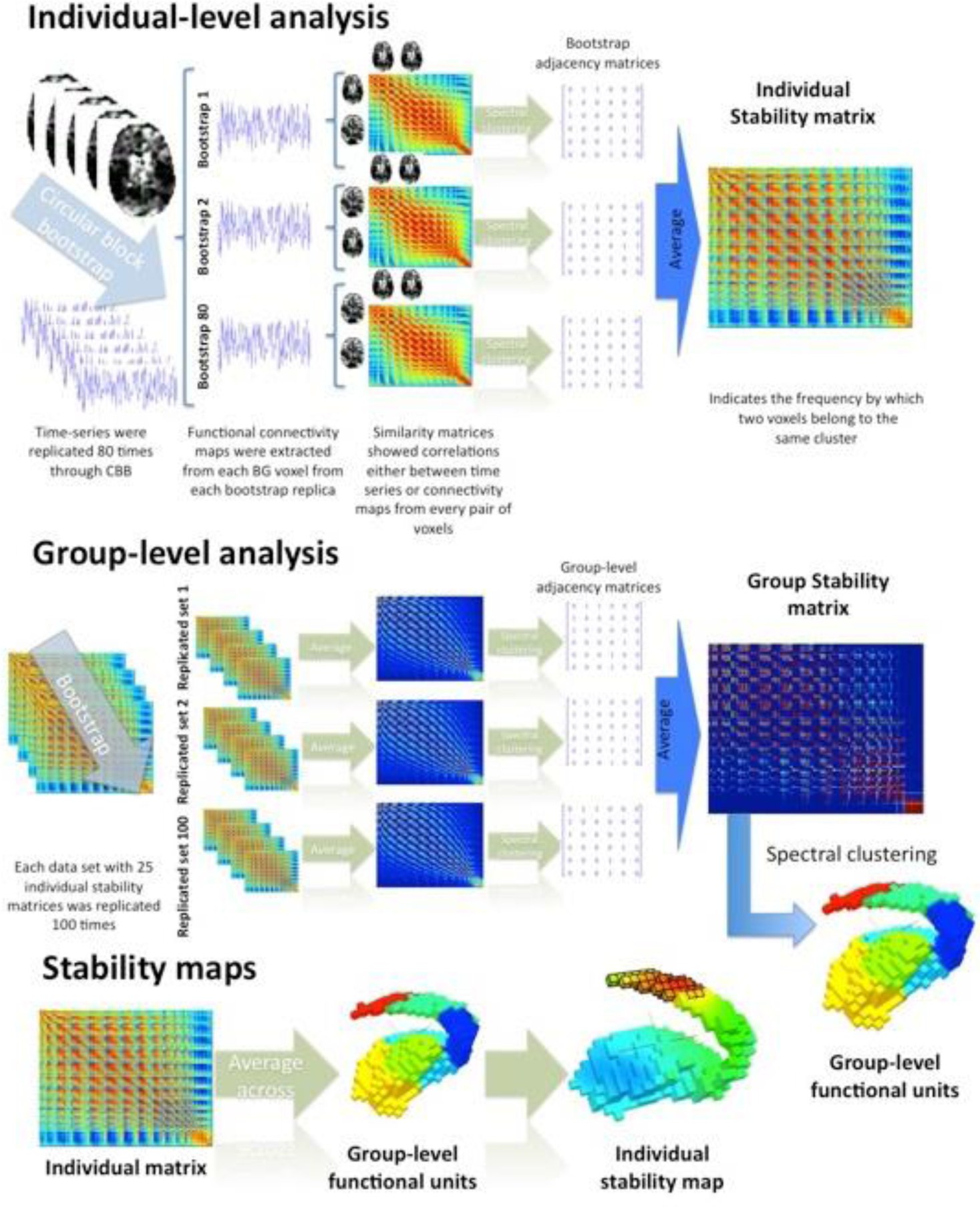
Analysis chart of BASC. Each individual’s time-series was sampled 80 times using circular block bootstrap. Whole-brain correlations were computed for every BG voxel at each replication, and similarity among all possible pairs of BG voxels was calculated using spatial and temporal correlations. Spectral clustering was then applied to derive clusters in resolutions from k=2 to k=9, and an adjacency matrix was created. Next, for each individual, the 80 adjacency matrices were averaged to create a stability matrix which quantifies the stability with which voxels were placed in the same functional unit across replications. To obtain group-level clusters, we generated 100 surrogate datasets featuring the same number of subjects as the original, and we derived an average stability matrix for each dataset. Each of the 100 stability matrices was then clustered, and a group stability matrix was generated. Finally, clustering was applied to the group stability matrix to produce a final set of group-level clusters. Stability maps were obtained for each individual by averaging the individual stability values across the voxels included in each group-level functional unit.

2.3.4. Stability Maps

Stability matrices depict the consistency with which two voxels are assigned to the same cluster. We can also estimate a stability map for a given functional unit that depicts the consistency of a voxel belonging to that cluster. An individual stability map can be calculated by combining the final stable cluster assignment with the individual stability matrix. For each voxel of the brain structure, the value in the stability map for a given functional unit is defined as the mean of stability values for that voxel and all the voxels within the given unit (Figure 1). Because the stability maps are based on the same group-level parcellation, individual differences in the stability for a given functional unit can be quantified by comparing the individual stability maps for that unit.

2.4. Implementation Specifics

The objective of cluster analysis is to partition a set of data points into k non-overlapping subsets such that observations assigned to the same subset are more similar to one another than observations assigned to different subsets. In the context of resting-state functional connectivity (RSFC), clustering algorithms have been used to partition voxels based on the similarity of whole-brain correlation maps (Craddock, James, Holtzheimer, Hu, & Mayberg, 2012; Kelly et al., 2010; Margulies et al., 2009) and on similarity of time courses (Bellec et al., 2010; Craddock et al., 2012). The methods have been applied to whole brain data in order to identify large-scale patterns of functional connectivity (Bernard et al., 2012; van den Heuvel, Mandl, & Pol, 2008) as well as with dimensionality reduction techniques to enable connectome analyses (Bellec et al., 2010; Craddock et al., 2012). Additionally, these methods have been applied within sub-regions of the brain in an attempt to identify fundamental sub-units of brain function (Kelly et al., 2010; Margulies et al., 2009).

Several parameters must be specified when performing a clustering analysis. The sub-region of the brain (or the entire brain) to be clustered must be defined. Additionally, a metric must be specified for measuring the similarity between voxels, and one of many different available clustering algorithms must be chosen. Here we constrain the clustering to the basal ganglia, and compare various metrics for measuring similarity, and different clustering algorithms as described in the following subsections.

2.4.1. Clustering Mask Definition

The basal ganglia was defined as the brain areas comprising putamen, caudate, nucleus accumbens and globus pallidus, obtained by setting a threshold of 50% on probability of belonging to these subcortical structures per the Harvard-Oxford Atlas (http://www.fmrib.ix.ac.uk/fsl/). We excluded the subthalamic nucleus and substantia nigra due to concerns regarding resolution. We focused our analyses on a single hemisphere to avoid the generation of non-contiguous clusters; given the high degree of similarity for connectivity patterns observed in homotopic areas of the striatum, we limited the scope of examination and reporting in the present work to the left hemisphere. The left hemispheric mask also enabled us to use more computationally extensive bootstrapping.

2.4.2. Similarity Metrics

We used two different metrics to measure similarity between voxels for clustering the BG (1438 voxels in the left BG). The spatial correlation (r_s) between two voxels was computed by the Pearson’s correlation of whole-brain connectivity maps derived from the voxel time series. Temporal correlation (r_t) between two voxels was measured by the Pearson’s correlation between their time series. Complementarily, we computed the eta2 statistic (1), which is identical to Pearson’s correlation for standardized variables but is shifted to be non-negative:

$${\mathit{\text{Eta}}}^2={\text{SumofSquares}}_{\mathit{\text{Between}}}/{\text{SumofSquares}}_{\mathit{\text{Total}}}$$ (1)

Before clustering, an r≥0.2 threshold was applied to r_s and r_t similarity metrics, which corresponds to a p<0.05 significance level calculated from the degrees of freedom of the fMRI time-series. By applying this threshold, we avoid negative and weak correlations contributing to the clustering analysis. Since functional units defined based on homogeneity of the RSFC maps and those obtained from BG voxels’ time-series yielded highly similar results, r_s was arbitrarily chosen to be reported in the main figures, but all the figures obtained with r_t are shown in the supplementary material.

2.4.3. Clustering Algorithm

Several approaches have been proposed for clustering R-fMRI data, such as normalized-cut spectral clustering (NCUT) (van den Heuvel et al., 2008), K-means (Mezer, Yovel, Pasternak, Gorfine, & Assaf, 2009), and hierarchical clustering (Goutte, Toft, Rostrup, Nielsen, & Hansen, 1999) (see Supplementary Figure 7). NCUT clustering has been shown to perform well at generating whole brain fMRI atlases based on spatially constrained spectral clustering on resting-state data (Craddock et al., 2012). As such, our primary analyses that focused on test-retest reliability and reproducibility exclusively used the NCUT algorithm for the individual- and group-level cluster analysis approaches. The spectral clustering (NCUT algorithm) Matlab toolbox by Verma & Meila (available at http://www.stat.washington.edu/spectral/) was specifically employed to partition each participant’s basal ganglia into k clusters.

2.4.4. Resolution Selection

Given the size of the brain region of 1438 voxels, a k range of 2 to 9 units was arbitrary chosen as results at higher resolution would be hard to interpret. We used a modified Silhouette index (MSI; 2) and the Davis-Bouldin index (3) to compare the performance of different clustering solutions within this range (k = 2 to 9). The modified Silhouette validation index (MSI) provides a measure of the similarity of voxels within a cluster to their similarity to voxels in other clusters:

$$S~\left(k\right)=\frac{\left(\mathit{\text{min}}\left(1-{\eta }_{\mathit{\text{bk}}}\right)\right)-\left(\mathit{\text{min}}\left(1-{\eta }_{\mathit{\text{wk}}}\right)\right)}{\left(\mathit{\text{max}}\left(1-{\eta }_{\mathit{\text{wk}}}\right)\right)-\left(\mathit{\text{min}}\left(1-{\eta }_{\mathit{\text{bk}}}\right)\right)}$$ (2)

In this equation, η_wk corresponds to the mean value describing the similarity between all voxels within a cluster, while η_bk corresponds to the K-1 mean values describing the similarity between all pairings of voxels within cluster k and voxels within other clusters. We also applied the Davis-Bouldin validation index (Davies & Bouldin, 1979):

$$\mathit{\text{DB}}\equiv 1/N\sum _{i=1}^N\mathit{\text{max}}\left(\left(S_i+S_j\right)/M_{i,j}\right)$$ (3)

In this equation, S_i is a measure of scatter within cluster i and M_i,j is a measure of separation between cluster i and j, and N corresponds to the number of clusters. The DB (Davis-Bouldin) index therefore corresponds to a ratio of the within-cluster distance to the mean distance between cluster centers, weighted by the number of clusters. Resolutions that represented local maxima for MSI and local minima for DBI are often identified as best performing resolutions.

2.4.5. Alternative Clustering Strategies

A key concern of any study employing clustering methodologies is the possible dependency of findings on the specific clustering algorithm or similarity measure employed. In order to address these concerns, we employed two alternative analytic strategies, one differing with respect to clustering algorithms (mimicking those initially used by Bellec et al., 2010) and the other differing with respect to the similarity measure employed (using eta2, similar to Cohen et al., 2008b; Kelly et al., 2012) (see Supplementary Figure 7).

2.5. TRT Reproducibility

Between-session reproducibility of BASC-derived stability matrices was estimated using the NYU TRT dataset, in which scans 2 and 3 were collected in a single session several months after scan 1. We also repeated our assessment of TRT reproducibility using the NKI TRT dataset. For the first measure of reproducibility, the Pearson correlation coefficient was calculated between each subject’s stability map calculated from scan 1 and the average of the stability maps calculated from scan 2 and scan 3.

The Dice coefficient (4) is the second measure of reproducibility that was employed, and was calculated between binarized stability maps calculated from scan 1 and the binarized map calculated from the average stability maps from scans 2 and 3. Stability maps were binarized by assigning the value 1 to a voxel for which the stability value was maximal across functional units, and a 0 to the same voxel in all other functional units. The Dice coefficient is calculated as the ratio of twice the number of connections common to both matrices, divided by the total number of connections present in both matrices:

$$\mathit{\text{dice}}=\frac{2\cdot \left|A-m\cap \mathit{\text{Am}}\right|}{\left|A-m\right|+\left|\mathit{\text{Am}}\right|}$$ (4)

Dice’s coefficient varies between zero and one, where one corresponds to perfect correspondence between matrices and zero corresponds to no similarity (Dice, 1945).

2.6. TRT Reliability

The TRT reliability of individual level BASC stability maps was estimated at the voxel level using intraclass correlation (ICC) (Shrout & Fleiss, 1979). For the NYU TRT dataset, we calculated ICC between the stability maps at scan 1 and stability maps from scans 2 and 3, which were averaged together to provide a more accurate estimate of functional connectivity, which is consistent with prior work (Shehzad et al., 2009; Zuo, Di Martino, et al., 2010; Zuo, Kelly, et al., 2010). In order to offer a more standard ICC demonstration we also applied ICC between scans 1 and 2 for the NKI TRT. To control for potential changes in the time courses produced by motion estimates from the data (Power, Barnes, Snyder, Schlaggar, & Petersen, 2012), we regressed the mean frame displacement out of stability maps for each session at the group-level before computing ICC. Here, ICC is used as an indicator of scanning reliability across sessions and defined as the proportion of variability between subjects relative to the total variability in the data. The calculation used here is a further extension of the classical definition of ICC varieties, which is based on linear mixed-effects modeling with restricted maximum likelihood (REML) estimates, which always generates non-negative ICC values (Zuo, Di Martino, et al., 2010).

2.7. Semantic Decoding

To interpret the functional significance of obtained clusters, we adopted the approach of Pauli et al., (2016) and used the Neurosynth meta-analytic decoder to generate a semantic map for the 5- and 9-cluster solutions. We used the decoder to list the top terms associated with each cluster, and created a list of the top terms across clusters. The radar plots in Figures 9 and 10 convey the relative commonality of each term for each BG parcel. For the five-cluster solution we chose the six terms with the highest representation in each cluster, as in Pauli et al. (2016), and for the nine-cluster solution we chose the three most represented terms per cluster.

Figure 9.

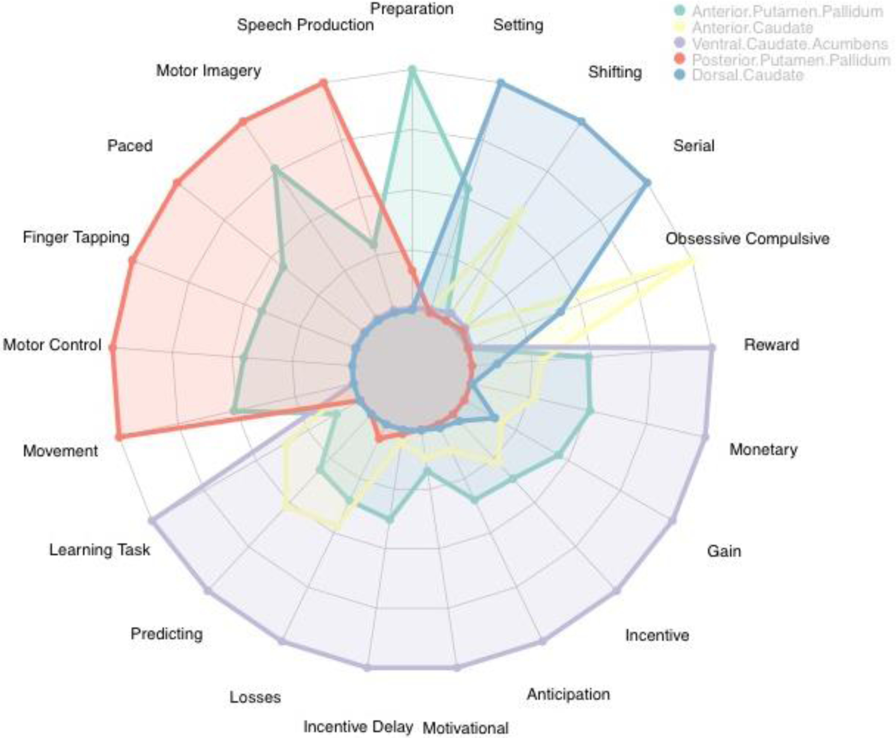
The radar plot shows the relative commonality of each term used in studies that included activation in one of the parcels in the 5-cluster solution. Clusters with values close to the center of the plot have low representation with that semantic label, while clusters in which coloration extends to the border of the plot have the highest relative presentation of the semantic label. We see that the semantic labels fall into categories that largely recapitulate the major discriminations of functions in the BG, including motor function in the posterior putamen, reward and goal oriented cognition in the ventral caudate and nucleus accumbens.

Figure 10.

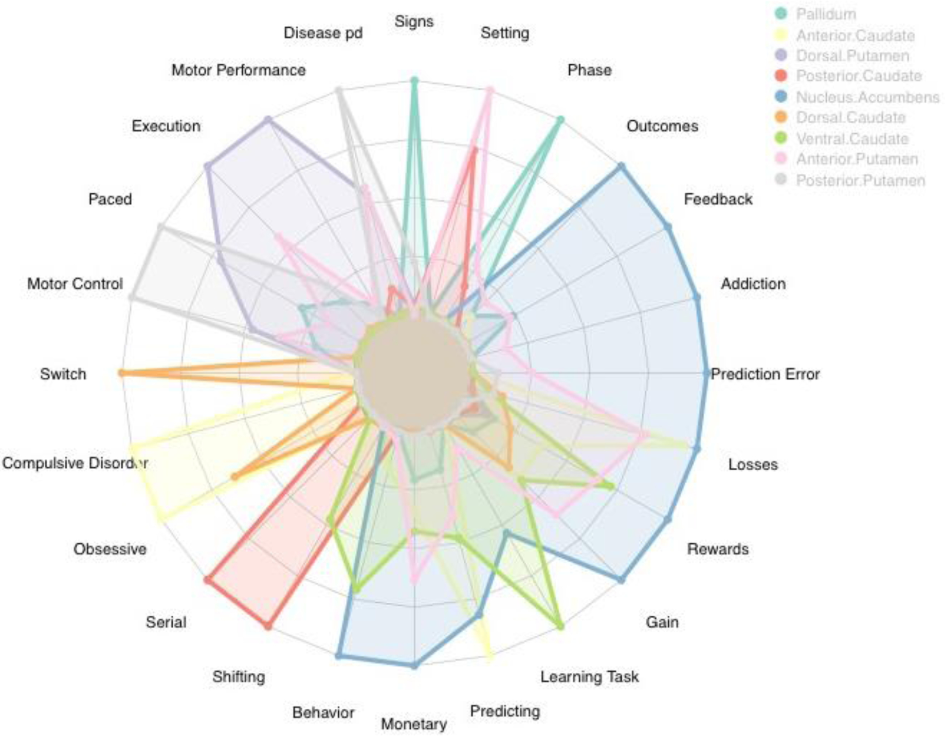
The radar plot shows the relative commonality of each term used in studies that included activation in one of the parcels in the 9-cluster solution. Clusters with values close to the center of the plot have low representation with that semantic label, while clusters in which coloration extends to the border of the plot have the highest relative presentation of the semantic label. We see that this solution demonstrates further delineation of semantic labels into sub-categories that may present more nuanced functional roles for each region.

3. Results

3.1. Functional Units and Resolution Selection

Using the multi-level BASC framework, we parcellated the BG into different functional units based upon the consistency of RSFC networks within and across individuals. Best performing cluster resolutions were selected using a combination of two independent metrics: the Davis-Bouldin Index measuring within-cluster dissimilarity, and the modified Silhouette Index measuring between-clusters dissimilarity. Determination of the best performing cluster number using the two approaches was facilitated by the high degree of concordance between resolutions that minimized the Davis-Bouldin Index and maximized the modified Silhouette Index. Regarding functional divisions based upon r_s, 2, 4, 8 and 9 were the best solutions for scan 1, while 2, 7 and 9 were the best solutions for scan 2, and 2, 5 and 9 performed best for scan 3. Similarly, for functional divisions based on r_t, 2, 4 and 9 were best performing resolutions for scan 1; 2, 7 and 9 for scan 2; and 2, 5 and 8 for scan 3. Because k=2 and k=9 were the most frequently repeated best performing solutions, and k=5 is the most descriptive mid-scale resolution of the resulting optimal outcomes, these 3 resolutions were selected.

Group-level cluster analysis of the BG in scans 1, 2 and 3 from the NYU TRT dataset led to similar functional units, regardless of whether they were based upon spatial (r_s) or temporal correlation (r_t) (see Figure 2 and Supplementary Material Figure 1). As Figure 2 shows, the caudate and putamen were divided across all cluster solutions, regardless of resolution, consistent with the primacy of this distinction suggested by anatomical and functional studies. While resolution k=5 divides the caudate into ventral, dorsal and anterior areas, the putamen is partitioned into anterior and posterior divisions. The k=9 resolution further segregates the nucleus accumbens from the caudate and the globus pallidum from the putamen, while maintaining the 3 caudate divisions of the k=5 resolution and dividing putamen into anterior, central, dorsal, and posterior units.

Figure 2.

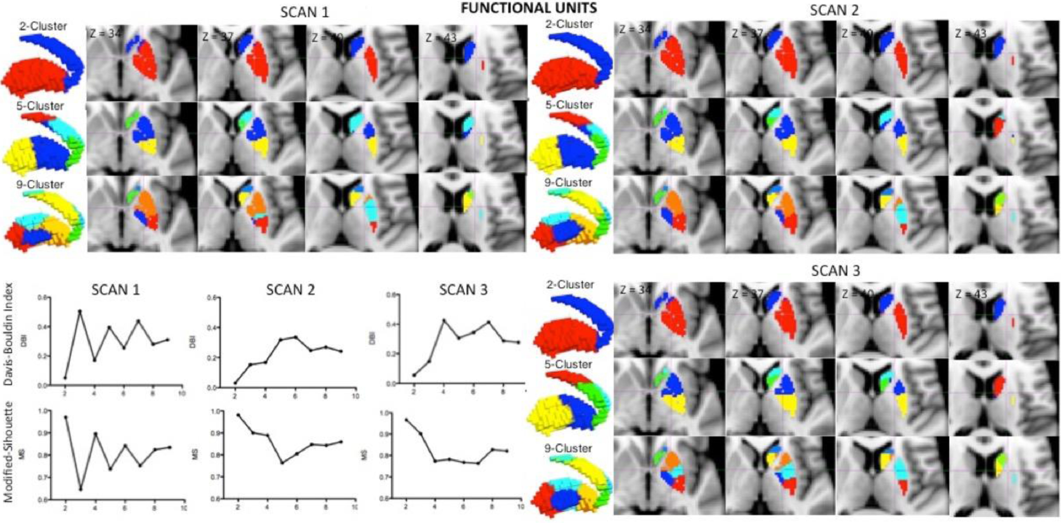
Functional parcellation units. The group-level parcellation of the BG in scans 1, 2 & 3 derive very similar functional units. The 3D renders and sagittal views reveal a main partition of caudate and putamen in k=2, that remain in every resolution. While resolution k=5 divides the caudate in ventral, dorsal and anterior areas into 2 units each, the putamen was sectioned into anterior and posterior units. The k=9 resolution showed a functional unit comprising nucleus accumbens and one for globus pallidum, while maintaining the tripartite caudate division of the k=5 resolution and dividing putamen into anterior, dorsal, central, and posterior units. Moreover, the Davis-Bouldin Index, a measure of within cluster dissimilarity, and the Modified-Silhouette Index, a measure of between-clusters dissimilarity, points to 2, 4, 6 and 8 as best performing solutions for scan 1, while 2, 7 and 9 for scan 2 and 2, 5 and 9 are the best performing resolutions for scan 3.

Given that k=2, k=5 and k=9 appeared to be the most appropriate resolutions across the r_s and r_t methods for the two validation indices, they are used in the following sections to assess stability, reproducibility and reliability of BASC for BG parcellation. The modular organization of these three resolutions and for both r_s and r_t revealed similar functional units across the three TRT sessions.

3.2. Mean Group Stability and Individual Variation

Figures 3a and 3b show the average of the stability maps across subjects for all clusters in resolutions k=2, k=5 and k=9 (target cluster is delineated by a white wireframe on the render and highlighted in the first column renders) for scans 1, 2 and 3. All three scans show similar mean stabilities, with highest values within the target cluster and lower values distant from it, regardless of whether the computation was based upon r_s or r_t. Likewise, to assess the variability of stability across subjects, we calculated the coefficient of variation defined as the standard deviation across participants divided by the average stability. Complementarily in the right part of Figures 3a and 3b, the maps show the coefficient of variation of the stability maps across subjects for all the target clusters in the resolutions k=2, k=5 and k=9. Again, scans 1, 2 and 3 show similar coefficients of variation, with lowest values within the target cluster turning into higher values for voxels distant from it.

Figure 3.

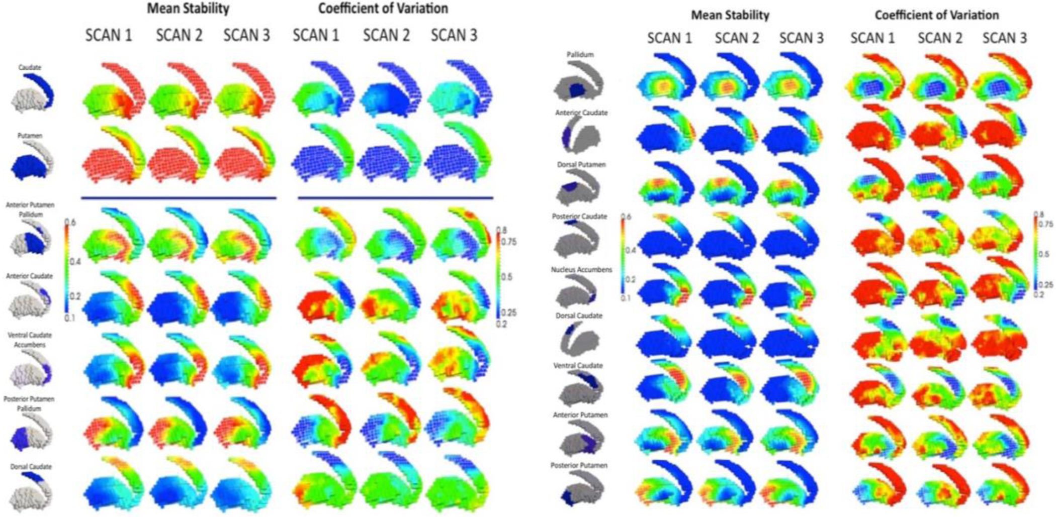
(A) Mean stability and coefficient of variation for resolutions k=2 and k=5. The panels and renders show the average of the stability maps across subjects for the 2 and 5 target clusters (shown on the first column renders and delineated by a white wireframe on the render) of the k=2 and k=5 resolutions. All three scans show very similar mean stabilities, with highest values within the target cluster and lower values distant from it. The right columns show the coefficient of variation (standard deviation relative to mean) of the stability maps across subjects for the 2 and 5 target clusters in the k=2 and k=5 resolutions. Again, all three scans show very similar coefficients of variation, with lowest values within the target cluster and higher values for voxels distant from it. (B) Mean stability and coefficient of variation for k=9 resolution.

We find that areas with greatest within-cluster mean stability also have the lowest coefficient of variation between individuals, suggesting that these clusters are stable both within and across individuals. While prior attempts at functional parcellation of the BG primarily used pooled group level data (Janssen et al., 2015; Kim et al., 2013), our group-level parcellation is comprised of individual-level cluster stability maps, and thus it demonstrates the consistency of our group solution at the individual level as well. In the two cluster solution, we find that the caudate-nucleus accumbens cluster separates cleanly from the putamen-pallidum cluster (Figure 3A). In the five cluster solution, we find a more detailed breakdown of these regions, but with some areas of lower within-cluster stability and greater between-subject variation. For example, we find that within both anterior and posterior putamen clusters, our results show that portions of the pallidum demonstrate lower stability and higher CV compared to the remainder of the cluster. We also find that the dorsal caudate shows relatively low mean stability compared to the other caudate clusters, which have mean stability values mostly > 0.8 and CV values ~ 0.2. In the nine cluster solution, the pallidum and nucleus accumbens broke into individual clusters, and each clustered region demonstrates selectively high mean stability and low CV in within-cluster voxels (Figure 3B). This suggests that compared to the lower resolution 5-cluster solution, the nine cluster solution may create clusters that are more easily separable from one another, and have better cluster coherence across individuals, making them better markers for investigating individual differences.

3.3. TRT Reproducibility

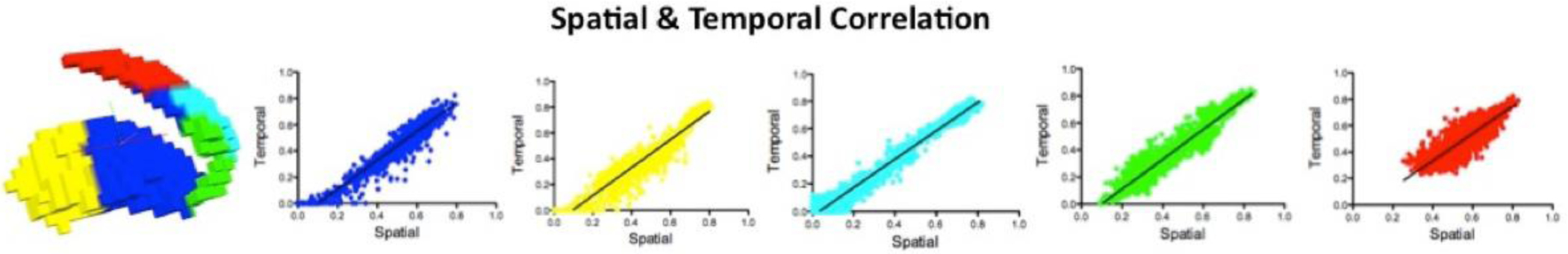
To quantify the extent to which the stability of the modular organization of the BG within an individual would be repeated if the resting state fMRI were collected at a different time, we used the NYU TRT dataset to compute the Pearson correlation coefficient and Dice coefficient between stability maps estimated from scan 1 and the average of those estimated from session 2 (the average of scans 2 and 3 was used to provide the best possible estimate of session 2). Figure 4 illustrates the reproducibility measured by Pearson correlation and Dice coefficient for each subject across stability maps obtained for resolutions k=2, k=5 and k=9; the colors of the scatter plots indicate the represented clusters. Most subjects showed reproducibilities between 0.6–0.9 as measured by both Pearson correlation coefficient and Dice coefficient. These data reveal moderate to high reproducibility of the stability maps obtained through BASC on r_s across different scans. While Figure 4 represents results obtained from r_s, Supplementary Figure 5 shows equivalent representations of reproducibility for the stability maps obtained by BASC on r_t. In sum, we found that the reproducibility indicated by Pearson correlations and Dice coefficients was moderate to high, with most subjects displaying values over 0.6.

Figure 4.

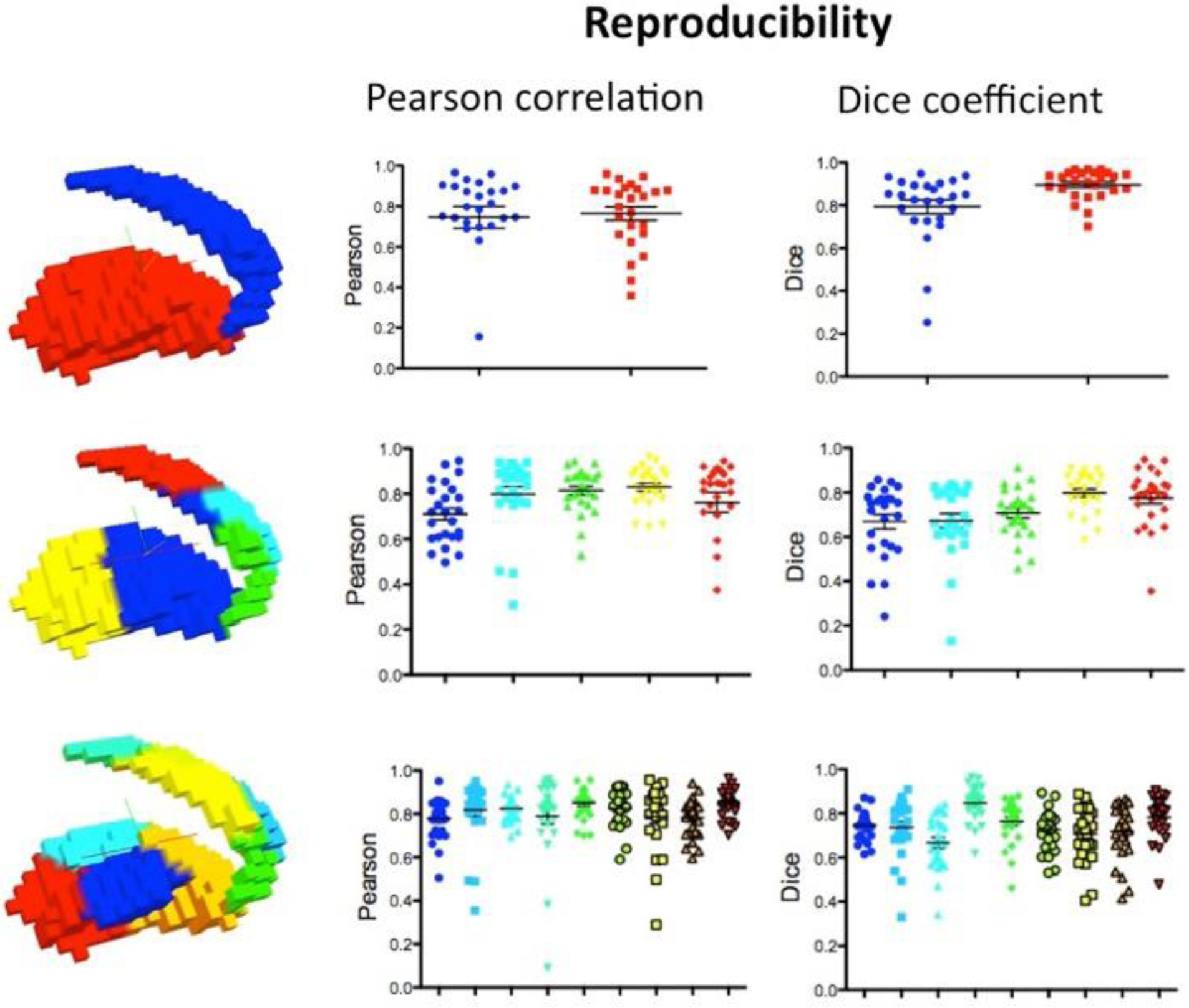
Reproducibility of stability maps. The 3D renders show the group-level functional units obtained for scan 2. The plots indicate the reproducibility measured by Pearson correlation for each subject across stability maps obtained for k=2, k=5 and k=9 resolutions. The Dice coefficients measured on binarized stability maps, in which 1 represents the most stable cluster, are also shown. These data reveal strong reproducibility of the stability maps obtained through BASC across different scans.

3.4. TRT Reliability

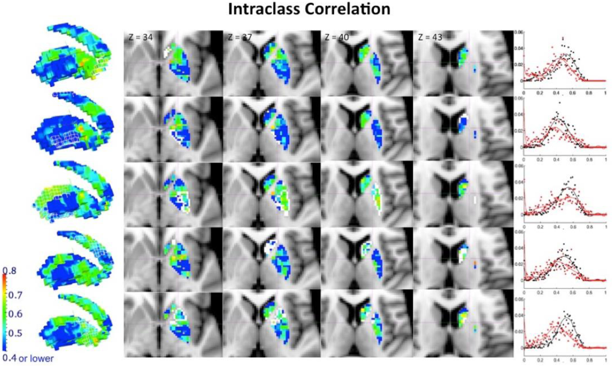
Similarly, to validate the utility of the BASC framework to study inter-individual differences in the stability of functional organization among regions, the NYU TRT dataset was also used to compute ICC at a voxel-level between stability maps obtained in scan 1 and the average of those obtained in session 2. TRT reliability showed a strong sensitivity to head motion effects. ICC values measured at a voxel level across the stability maps obtained for scan 1 and the averaged stability map of scans 2 and 3 for resolution k=5 are shown in Figure 5 (target clusters delineated by a white line for the slice view and a white wireframe on the render). Figure 6 shows ICC maps for resolution k=9. The graph placed next to each cluster’s ICC map represents the distribution of frequencies of the ICC values obtained when ICC was computed after having regressed out mean frame displacement for each subject (in black), and also when ICC was calculated without regressing that parameter out (in red).

Figure 5.

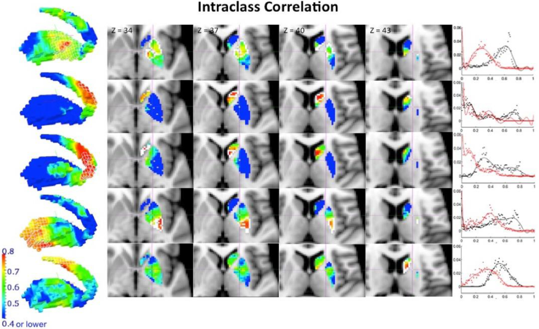
Reliability of the stability maps measured by the intraclass correlation (ICC). We examined reliability at every voxel level through ICC in the stability maps, defined as the proportion of variability across subjects relative to the total variability in the data. The calculation used here is a further extension to the classical definition, which is based on linear mixed-effects modeling with restricted maximum likelihood estimates, that always generates all non-negative ICC values. ICC values between the stability maps obtained from scan 1 and the average of scans 2 and 3 at k=5 resolution are shown here (target clusters are delineated by a white line for the slice view and a white wireframe on the render). High ICC values are only found in proximity to the target cluster. The graph placed next to each cluster’s ICC map represents the distribution of frequencies of the ICC values obtained when ICC was computed after having regressed out mean frame displacement for each subject (in black), and also when ICC was calculated without regressing that parameter out (in red).

Figure 6.

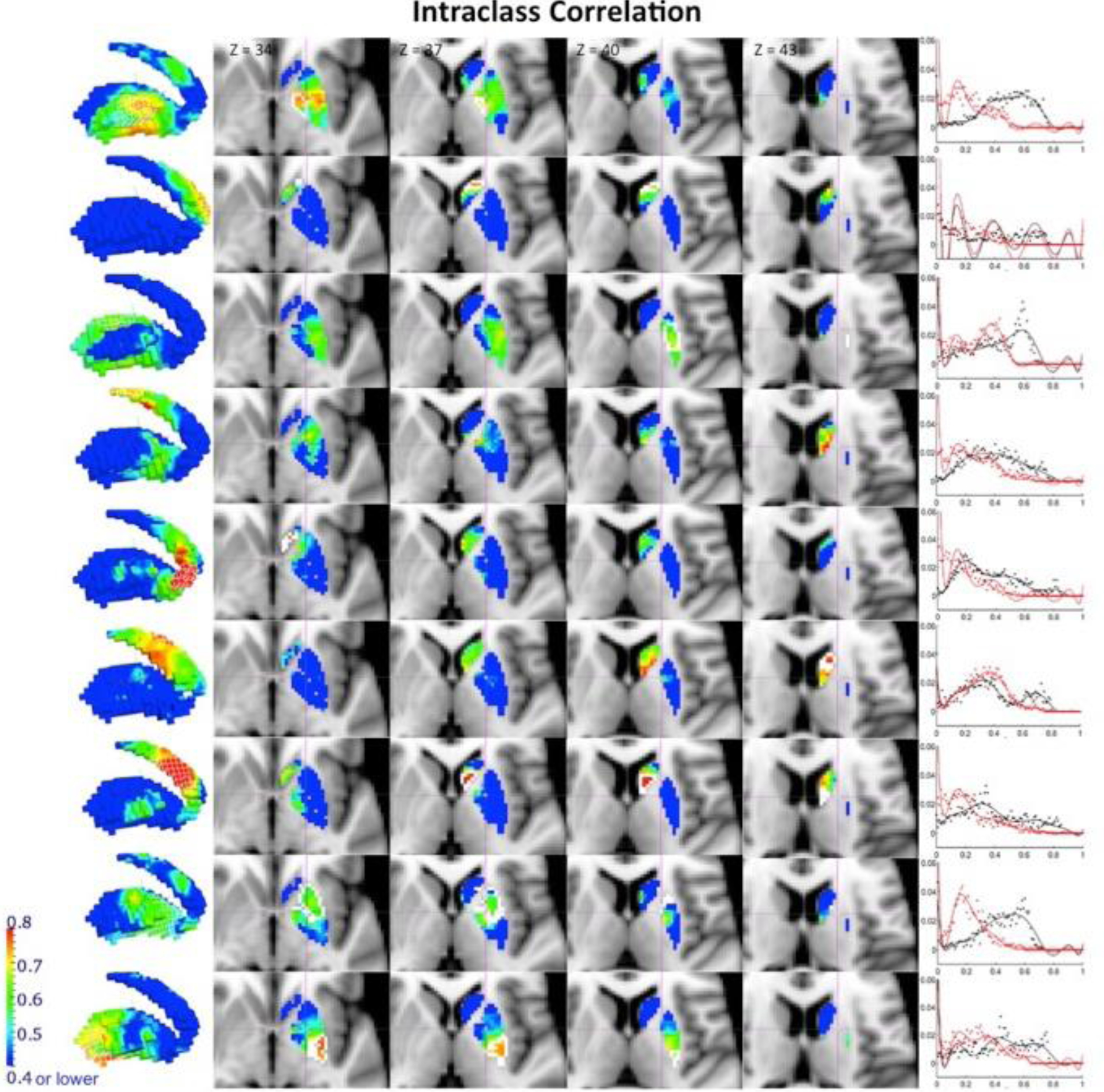
Reliability of the stability maps measured by the ICC. ICC values between the stability maps obtained from scan 1 and the average of scans 2 and 3 at resolution k=9 are shown here (target clusters are delineated by a white line for the slice view and a white wireframe on the render). High ICC values are only found in proximity to the boundaries of the target cluster. The low between-subject variability shown by the coefficient of variation within the target cluster, as well as the low stability in voxels distant from the target cluster might explain this regional distribution of ICC values in the BG, where the boundaries show enough within-subjects stability as well as between-subject variability to allow for a proportion of variability across subjects to be significant across the total variability of the data. The graph placed next to each cluster’s ICC map represents the distribution of frequencies of the ICC values obtained when ICC was computed after having regressed out mean frame displacement for each subject (in black), and also when ICC was calculated without regressing that parameter out (in red).

It is interesting to note the regional specificity of high ICC values. These are particularly found both near the boundaries of the target cluster and within the target cluster. Despite the low between-subject variability shown by the coefficient of variation within the target cluster, TRT reliability is shown to be high in these areas, representing that a high proportion of the total variability across subjects is explained by high between-session correlation within each individual. However, the low stability in voxels distant from the target cluster combined with high between-subject variation might contribute to the low ICC values in BG areas located far from the target cluster. Therefore, the boundaries and target clusters show enough within-subject stability as well as between-subject variability to allow for a proportion of variability within subjects to be significant across the total variability of the data. TRT reliability and ICC value distributions were equivalent for corresponding clusters in results obtained from r_s and those obtained from r_t (see Figure 7). While Figures 5 and 6 report results obtained from r_s, Supplementary Figures 4 and 5 show similar figures for results obtained from r_t. To further demonstrate the TRT reliability and generalizability of this technique, Supplementary Figure 6 shows the ICC obtained by applying BASC to the medial wall of the frontal cortex. We see ICC values > 0.6 within each cluster and in regions proximal to the clusters. These results demonstrate that high ICC values can be obtained in cortical regions as well, suggesting that BASC is capable of deriving stable and reproducible clusters on an individual level.

Figure 7.

The plots show the correlation between the ICC values obtained from the spatial correlation similarity measure and those obtained from the temporal correlation similarity measure for each of the five clusters with resolution k=5. The colors of the scatter plot points match the cluster colors.

Given the availability of the multiband NKI TRT dataset with a rapid TR of 645 ms, we repeated our ICC analysis on this dataset to evaluate the impact on cluster stability of higher temporal resolution (and additional observations) afforded by this emerging technology. Consistent with the reliability measure on the NYU TRT, Figure 8 confirms the pattern shown by Figures 5 and 6 in a multiband TRT dataset with a TR of 645 ms: high ICC values were particularly found in proximity of the boundaries of the target cluster as well as within the target cluster. Consistent across methods and datasets, high reliability of the stability measures obtained through the BASC framework was found particularly within the target unit and on the boundaries of that unit.

Figure 8.

Reliability of the stability maps measured by ICC in a multi-band dataset with a rapid TR of 645 ms for a different TRT sample. ICC values between sessions 1 and 2 for the stability maps derived from the resolution k=5 are shown. Target clusters are delineated by a white line for the slice view and a white wireframe on the render. High ICC values are again only found in the proximities of the boundaries of the target cluster. The graph placed next to each cluster’s ICC map represents the distribution of frequencies of the ICC values obtained when ICC was computed after having regressed out mean frame displacement for each subject (in black), and also when ICC was calculated without regressing that parameter out (in red).

3.5. Semantic Mapping

To facilitate interpretation of the clusters obtained, we display semantic loadings for each cluster in Figures 9 and 10, obtained using the Neurosynth meta-analytic semantic decoder (Pauli et al., 2016; Yarkoni, Poldrack, & Nichols, 2011). For the five-cluster solution, each region is largely associated with one or more of the major functions of the BG commonly reported in the literature (e.g., reward and value, motor movement). In the nine-cluster solution we see a further differentiation of motor control from motor execution in the posterior and dorsal putamen, respectively, and this solution also recapitulates expected functions of the BG, such as valence, reward and error processing in the nucleus accumbens and ventral and anterior caudate clusters.

4. Discussion

4.1. Reliability of Individual-Level and Group Parcellations

Establishing reliable functional atlases at the individual level is a critical step towards understanding both function-anatomy associations and relationships between variations in both cognitive and clinical phenotypes and functional network architecture. The present work demonstrates a method for establishing such reliable parcellations at the individual level. Specifically, our quantification of test-retest reliability and reproducibility of findings obtained with the BASC framework, over the short- and long-term, supports its ability to capture inter-individual differences in the functional subdivisions within complex brain structures, such as the BG (Chang & Glover, 2010). In particular, our findings demonstrate that high mean stability also exists at the borders between subdivisions (Figures 3A & 3B). This finding is supported by recent parcellations highlighting the greatest source of individual variance in parcellations lies at the boundaries of parcels (Xu et al., 2016). Importantly, as the number of clusters in a solution increased, we found notable variation among clusters with respect to the distribution of maximal mean stability (e.g., within the cluster, surrounding regions, distant region; Figure 3B), highlighting the importance of assessing reliability before applying these approaches to a particular region of interest. The clusters created through BASC were not only highly stable within participants, but also reliably stable across participants, as demonstrated by low within-cluster coefficient of variation (Figure 3A, 3B), enabling more accurate between-subject comparisons of BG clustering. Therefore, such parcellations derive reliable indicators of individual differences in BG connectivity, and such parcellations may be used in further work to more reliably assess how phenotypic differences manifest in the basal ganglia.

We found moderate to high reproducibility between sessions for the BASC framework, providing further support for the assertion that these parcellations are stable indicators of individual differences in the BG. We also found that between-sessions reliability revealed an interesting regional distribution specific for the target cluster and the unit’s boundaries. This regional distribution of highly reliable voxels in the maps suggests that the consistency of the functional organization within a given functional unit, as well as in the boundaries between functional units indicated by sharp changes in their FC patterns (Cohen et al., 2008a), contain information that is stable and distinctive from other individuals (Figure 5 & 6). This is particularly exciting given that modules’ boundaries do not seem to follow structural variation but rather differences in functional task-related activity (Cohen et al., 2008a; Mennes et al., 2010), behavior shown by phenotypic variables (Chabernaud, Mennes, Kelly, & Nooner, 2013; Cox et al., 2012; Di Martino, Ross, et al., 2009; Di Martino, Shehzad, et al., 2009; Koyama et al., 2011) and development (Kelly et al., 2009). This pattern of high reliability (ICC>0.5) within the target cluster and on the transition zones was replicated on a different test-retest sample with a faster TR (645 ms; see Figure 8). This replication is a strong demonstration of the reliability of this technique.

4.2. Validation of Prior Work

Based upon data-driven cluster analysis approaches, the BASC framework successfully recapitulated previously observed BG subdivisions (Barnes et al., 2010; Di Martino et al., 2008), while providing a greater degree of detail and simultaneously assessing their reliability at the individual level. The 5-cluster parcellation of the BG into body and tail of the caudate, nucleus accumbens, and anterior and posterior putamen is consistent with results from invasive tracing studies in nonhuman primates (Haber, 2003; Künzle, 1977). This solution is also consistent with a BG parcellation calculated using probabilistic tractography of diffusion-weighted MRI data (Draganski et al., 2008). It is also consistent with R-fMRI functional connectivity analyses that found markedly different functional connectivity patterns for superior and inferior ventral striatum and dorsal caudate, seeds that fall into different functional units in the 5-cluster solution (Di Martino et al., 2008).

Our parcellation also supports and extends previous attempts to segment the BG using R-fMRI (Barnes et al., 2010). For example, our high resolution 9-cluster solution was able to reliably delineate regions of the BG with similar global connectivity patterns, splitting the nucleus accumbens from the caudate, the globus pallidus from the putamen, and refining the putamen into four distinct regions: anterior, posterior, dorsal, and central putamen. Our stability maps also demonstrate the reliability of each of these parcels, suggesting that these more detailed separations are not only anatomically coherent, but may also reflect a more detailed differential pattern of global connectivity between neighboring areas of the BG that are not commonly analyzed separately (Barnes et al., 2010; Di Martino et al., 2008). Furthermore, the stability of each region in the 9-cluster solution was equal to or better than the 5-cluster solution. Given that prior work has demonstrated decreasing stability in clustering at higher resolution (Craddock et al., 2012), our results suggest that the 9-cluster solution offers a depiction of BG connectivity patterns that are more reliable and accurate than prior depictions, and these cluster solutions are highly stable and conserved at the individual level.

Our results also demonstrate that the stability of these clustering solutions holds regardless of whether voxels were clustered according to similarity of their timeseries (r_t) or similarity of their connectivity maps (r_s). Our results were replicated in Supplementary Figure 5, with Figure 7 directly assessing the similarity between the r_t and r_s results. The multi-level BASC method comprises a group-level analysis that bootstraps the set of all individual stability matrices (Bellec et al., 2010). The goal of this second level of bootstrapping is to obtain a group-level stability matrix that contains only the most stable voxel pairings, thus assuring homogeneity at a group-level, based on homogeneity at an individual-level. Obtaining such highly reproducible clustering solutions is important for both scientific and clinical endeavors. We found that stable clusters obtained from the multi-level BASC described almost identical functional organizations across scans, which supports the reliance on this method to define the organization of a brain area based on the most stable clusters both across and within subjects. To test the consistency of the group-level solutions across sessions we computed the Dice coefficient of group level stability maps, obtaining values of 0.99, 0.86 and 0.90 for the k=2, 5 and 9 resolutions, respectively. Highly reproducible findings across scans reflect low measurement error, which enables us to more accurately detect cross-sectional differences ascribable to underlying disease etiology rather than to measurement artifact. Furthermore, we can examine longitudinal changes more accurately that occur as a result of treatment because treatment or development-induced changes are less likely to be conflated with measurement noise.

4.3. Reliability Across a Range of Methods

The BASC framework is flexible with respect to the specific cluster analysis approach employed. This configurability makes the framework particularly appealing, though different implementations may influence findings, increasing the need to compare the reliability of different implementations. An array of alternative cluster analysis and data reduction approaches exists. For example, in our supplementary analyses we compared findings from spectral clustering to k-means and hierarchical clustering approaches – two of the most common algorithms. While all had moderate to high test-retest reliability, spectral clustering resulted in the highest ICC values. A potential concern with the spectral clustering method used is the potential for a bias towards creating clusters of similar size in regions of the brain where a clear clustering is not obvious (Craddock et al., 2012). In the present work, this did not appear applicable as the organization of the BG at the group-level resulted in functional units of different sizes with good anatomic validity. Further, the group-level NCUT results bore a striking similarity to those obtained with other approaches.

Beyond selection of the cluster algorithm, another key decision was the similarity measure. In particular, one needs to decide between temporal and spatial indices of similarity, which were quantified with correlation in the present work. While Craddock et al. (2012) indicated that spatial and temporal correlations differ in their distribution as well as in their validation indices, our findings suggest that such differences have minimal effect on reproducibility and reliability in the context of clustering the BG. In fact, Figure 7 directly compared ICC values for corresponding functional units in the temporal and the spatial analyses, yielding high correlations. Moreover, the stability maps, coefficients of variation and parcellations appeared to be equivalent when obtained through spatial and temporal similarity. This aligns also with the Craddock et al. 2012 findings, which demonstrated that while the correlation distributions can be quite different, using r_s or r_t had minimal impact on the cluster solutions themselves. Arbitrarily, our spatial similarity results are displayed on the main figures and temporal results in the supplementary material. However, in terms of computational cost, we recommend the use of temporal similarity for further application of the BASC framework.

An alternative to correlation as a similarity index is the eta2 statistic (Cohen et al., 2008a). This statistic is identical to Pearson correlation for standardized variables but it is shifted to be non-negative and maintains scalar differences. Although group-level results obtained with eta2 were comparable to those obtained with correlation, examination of inter-individual differences using ICC suggested that eta2 engendered markedly lower reliabilities (see Supplementary Material Figure 7). Future work should investigate alternative metrics of similarity (e.g., concordance correlation coefficient).

Another key decision in the BASC framework is the selection of graph construction algorithms. The work of Craddock et al. (2012), upon which our clustering strategy was based, used an epsilon neighbor approach, for the explicit purpose of ensuring contiguous clusters, given their focus on identification of functional units. Although justified in their application, for the purposes of the present work such a constraint would decrease the biological plausibility of findings. Moreover, spatial constraints are not optimal while delineating functional boundaries (Cohen et al., 2008b; Kelly et al., 2010) because a functional network comprises regions with homogeneous FC patterns without any spatial restriction. Similar to the findings of Craddock et al. (2012), we found only contiguous clustering. One caveat is that we analyzed the left hemisphere exclusively; had right and left BG been included in the same analysis with a fully connected graph, strong homotopic connectivity patterns would have undoubtedly emerged.

Power and colleagues (2012) demonstrated that subject motion produces substantial artifactual changes in the time-courses of RSFC data, even after compensatory spatial registration and regression of motion estimates. Many long-distance correlations are decreased by subject motion, while short-distance correlations are increased. To avoid artifacts introduced by micro-movements in the different sessions, the mean frame displacement (FD) was regressed out of the stability maps of every individual. We performed an additional analysis without this regression to evaluate the impact of movement on the between-sessions ICC values produced by the BASC framework. The plots in Figures 5, 6 and 8 show an improved ICC for mean FD regression, compared to results that did not include this procedure. Thus, taking into account micro-movements improves the reliability of inter-individual differences in the brain functional organization of iFC networks.

4.4. Limitations and Future Directions

Prior work has raised concerns about the potential for signal bleed that can impact findings (Choi et al., 2012; Curtis, Hutchison, & Menon, 2014). Unfortunately, to date, there is not an optimal or established approach for accounting for and removing this phenomena. While a regression-based approach was recently suggest, the authors noted this to be an imperfect solution; an ample space of possibilities for correction exist, and their impact on the validity and reliability of findings is yet to be established. Future work would benefit from comprehensive testing and evaluation of the impact of bleeding and correction strategies. Given the role the basal ganglia plays in the development of a range of motor, cognitive, and affective functions, another important future application of BASC could be in the assessment of BG clusters over child and adolescent development, as the executive, attention, and limbic networks mature into their adult phenotypes. We expect that BASC may offer important insight into the reorganization of the BG that mirror the significant cognitive development that occurs during this time period. Prior work has also demonstrated that the connectome displays significant state-sensitivity (Craddock et al., 2013; Mennes, Kelly, Colcombe, Castellanos, & Milham, 2013). Therefore, an important avenue of future work would be to apply BASC on the basal ganglia during rest to a range of motor, executive, attention tasks. We expect that clustering the BG based on single networks may be specifically sensitive to task demands. Furthermore, important individual differences may lie in the stability of these cluster solutions, for example cluster, cluster stability may be associated with individual differences in network dynamics that play a role in a range of cognitive processing (Byrge, Sporns, & Smith, 2014; Cole et al., 2013; Nikolaidis & Barbey, 2016). Future work should therefore interrogate how individual differences in reproducibility across individuals also vary across regions and whether these differences are associated with cognition as well.

5. Conclusion

Reliable Individual-level mapping of the functional architecture of the brain is a critical step towards understanding complex cognitive systems and developing biomarkers and treatments in a wide range of clinical domains. The present study provides support for using BASC to quantify inter-individual differences in the functional organization of regions of interest. Demonstration of test-retest reliability satisfies a prerequisite for future work attempting to relate variations in each region’s modular organization, behavioral traits, experimental manipulations of state, development, aging or psychopathology (e.g., Attention Deficit/Hyperactivity Disorder, Autism Spectrum Disorder or schizophrenia, even from the first psychotic episode).