Future Fire Impacts on Smoke Concentrations, Visibility, and Health in the Contiguous United States

Abstract

Fine particulate matter (PM_2.5) from U.S. anthropogenic sources is decreasing. However, previous studies have predicted that PM_2.5 emissions from wildfires will increase in the midcentury to next century, potentially offsetting improvements gained by continued reductions in anthropogenic emissions. Therefore, some regions could experience worse air quality, degraded visibility, and increases in population‐level exposure. We use global climate model simulations to estimate the impacts of changing fire emissions on air quality, visibility, and premature deaths in the middle and late 21st century. We find that PM_2.5 concentrations will decrease overall in the contiguous United States (CONUS) due to decreasing anthropogenic emissions (total PM_2.5 decreases by 3% in Representative Concentration Pathway [RCP] 8.5 and 34% in RCP4.5 by 2100), but increasing fire‐related PM_2.5 (fire‐related PM_2.5 increases by 55% in RCP4.5 and 190% in RCP8.5 by 2100) offsets these benefits and causes increases in total PM_2.5 in some regions. We predict that the average visibility will improve across the CONUS, but fire‐related PM_2.5 will reduce visibility on the worst days in western and southeastern U.S. regions. We estimate that the number of deaths attributable to total PM_2.5 will decrease in both the RCP4.5 and RCP8.5 scenarios (from 6% to 4–5%), but the absolute number of premature deaths attributable to fire‐related PM_2.5 will double compared to early 21st century. We provide the first estimates of future smoke health and visibility impacts using a prognostic land‐fire model. Our results suggest the importance of using realistic fire emissions in future air quality projections.

Key Points

• We provide the first estimates of future smoke health and visibility impacts in the contiguous United States using a prognostic land‐fire model

• Average visibility will improve across the contiguous United States, but fire PM will reduce visibility on the worst days in western and southeastern U.S. regions

• The number of deaths attributable to total PM_2.5 will decrease, but the number attributable to fire‐related PM_2.5 will double by late 21st century

1. Introduction

Exposure to particulate matter (PM_2.5, particles with an aerodynamic diameter smaller than 2.5 μm) is associated with many negative health impacts (Crouse et al., 2012; Krewski et al., 2009; C. Arden Pope, 2007; C Arden Pope 3rd & Dockery, 2006), visibility degradation, and ecosystem impacts. There are many different sources of PM_2.5, both from human and natural sources. Because of the known detrimental effects of air pollution, the United States has sought to improve air quality through regulation of anthropogenic emissions. This has led to PM_2.5 improvements in most regions of the United States (e.g., Hand et al., 2013; Malm et al., 2017; U.S. Environmental Protection Agency (EPA), 2012). These PM_2.5 improvements are predicted to increase in the future with a further decrease in anthropogenic emissions (e.g., Lam et al., 2011; Leibensperger et al., 2012; Val Martin et al., 2015).

Wildfires are a large source of PM_2.5 in the United States, and studies have shown that the number of large wildfires has been increasing in the western United States due to warmer temperatures, earlier spring snowmelt, and longer fire seasons (e.g., Westerling, 2016; Westerling et al., 2006). Several studies have suggested that this trend will continue throughout the 21st century and that smoke could become the dominant source of PM_2.5 in the western United States during the fire season (e.g., (Liu et al., 2016; Yue et al., 2013). However, estimating future fire emissions and their impact on air quality is challenging. Fire trends are influenced not only by the changing climate but also by land use changes, land management choices, and human interactions (in terms of both ignition and suppression; e.g., Balch et al., 2017; Fusco et al., 2016; Prestemon et al., 2013). Most studies that have estimated future fires (risk or area burned) have relied on statistical regressions of current‐day meteorological values (such as precipitation, relative humidity, and temperature) and fire indices (Liu et al., 2016; Prestemon et al., 2016; Spracklen et al., 2009; Westerling & Bryant, 2008; Yue et al., 2014), or parameterizations built off these statistical regressions (Liu et al., 2016; Yue et al., 2013, 2014) showed that these methods are able to explain 25–65% of the variance in area burned, but the efficacy is regionally dependent. When applied to future predictions, these studies suggest increases in fire emissions, specifically in the western United States, leading to increases in surface fire‐related PM concentrations (Spracklen et al., 2009; Yue et al., 2013), visibility degradation (Spracklen et al., 2009), and smoke‐exposure events (Liu et al., 2016). Val Martin et al. (2015) previously used Community Earth System Model (CESM) to simulate future PM concentrations in the United States with regard to changing emissions, land use, and climate. For fire emissions, they used the spatial distributions from the Representative Concentration Pathway (RCP) scenarios and then homogeneously scaled the monthly emissions in the western United States and Canada to match the total fire emissions from Yue et al. (2013).

More recently, process‐based fire modules embedded in global land models have been used to estimate future fires and emissions (e.g., Knorr et al., 2017; Pierce et al., 2017). These fire modules use information on both climatic and socio‐economic drivers (e.g., soil moisture, temperature, gross domestic product, and population density) to estimate area burned and fire emissions (Knorr et al., 2014; Li et al., 2013; Pierce et al., 2017). In contrast to statistical models, processed‐based fire models can better represent feedbacks between emissions and climate and land use (Li et al., 2012, 2013, 2017). Additionally, they do not have to assume that the statistical relationships determined from current day observations will stay the same in the future under different climate scenarios nor do we need to either assume a statistical relationship holds for all regions or create a statistical relationship for each region. Finally, using the process‐based fire module within a global model allows us to account for changes in fire emissions outside the study domain (contiguous United States) that can also impact air quality within our study domain. In this study, we use simulated concentrations of PM_2.5 generated by the CESM for early 21st century (“2000,” the average of 2001–2010), midcentury (“2050,” average of 2041–2050), and late 21st century (“2100,” average of 2091–2099) described in Pierce et al. (2017) to estimate changes in PM_2.5 concentrations, population‐level exposure, health effects, and visibility in the United States.

2. Methods and Tools

2.1. Model Simulations of Fire Emissions and Atmospheric Concentrations

We use the CESM to simulate surface‐level PM_2.5 concentrations. A description and evaluation of the model is given in Tilmes et al. (2015). The model is run at 0.9° × 1.25° horizontal resolution for three periods: early 21st century (2000–2010), midcentury (2040–2050), and late century (2090–2099). Results are shown as 10‐year averages (with the first year excluded for model spin‐up). Ten‐year time periods were run to represent climatological averages and account for interannual variability. The simulations were conducted in two separate steps: (1) simulating fire emissions using a land model and then (2) simulating air quality impacts using an atmospheric model.

First, emissions for landscape, agricultural, and peat fires were interactively simulated using the Community Land Model (CLM) v4.5 (Oleson et al., 2013), which accounts for changes in land cover, vegetation, climate change, and population (Pierce et al., 2017). These runs were conducted globally at 0.9° × 1.25° resolution for 1850 to 2100. Future fire simulations (2006–2100) were driven by monthly meteorological fields from archived CESM1 simulations with the RCP4.5 and RCP8.5 scenarios and population projections from the Shared Socioeconomic Pathways (SSPs; Jones & O'Neill, 2016); the transition period (1850–2005) was forced with assimilated atmospheric data from the Climatic Research Unit of the National Centers for Environmental Prediction (CRUNCEP) and population data from the History Database of the Global Environment (HYDE). The transient run started from an 1850 equilibrium (spin‐up) state of CLM4.5 with the fire module. Description of the original fire module and comparison with fire emission inventories are given in Li et al. (2012), and updates to the module and further validation are in Li et al. (2013) and Li et al. (2017). Li et al. (2013) and Li et al. (2017) found that CESM with the updated fire module is able to simulate the spatial distribution of fires, total area burned, fire seasonality, fire interannual variability and trends, and fire carbon emissions reasonably well compared to observations.

Second, the Community Atmospheric Model v4 fully coupled with an interactive gas‐aerosol scheme (CAM‐Chem) was used to simulate air quality impacts (Lamarque et al., 2012) using the fire emissions from the CLM. Meteorology in our present‐day CAM‐Chem simulations is free‐running and not assimilated for present day. Hence, specific daily meteorological conditions in the present‐day simulations do not correspond to observed conditions. Population projections are taken from the SSPs (Jones & O'Neill, 2016) and are described in detail in section 2.2. Biogenic emissions were determined using the Model of Emissions of Gases and Aerosols from Nature (MEGAN v2.1; Guenther et al., 2012). For estimating future anthropogenic emissions, we used the RCP scenarios 4.5 and 8.5 (van Vuuren et al., 2011). The RCPs are four different future climate scenarios that describe trajectories for greenhouse gas concentrations. They are referred to by the associated amount of radiative forcing that would occur by 2100 compared to preindustrial times (i.e., RCP4.5 corresponds to a +4.5 W/m² forcing). The RCP8.5 scenario assumes continued increases in greenhouse gas concentrations throughout the 21st century due to high populations, slow income growth, high energy demand with moderate technological changes to reduce emissions, and the absence of climate change policies. In RCP8.5, methane and carbon dioxide emissions will increase throughout the century. The RCP4.5 pathway has a gradual reduction in greenhouse gas emission rates after 2050 such that radiative forcing is stabilized shortly after 2100. It assumes a shift to lower emission energy sources, enactment of climate policies, less croplands, and more forests. In RCP4.5, carbon dioxide emissions will increase to midcentury and then decline; methane emissions will have a slight decline throughout the century. Both scenarios suggest a decrease in SO₂ and NO_x emissions (although a greater decline in NO_x emissions with the RCP4.5 scenario).

Fire emissions were provided to CAM‐Chem from the CLM4.5 fire simulations described above. We note that due to internal variability in climate dynamics, an ensemble of CESM simulations could potentially provide a range of potential future smoke PM_2.5 concentrations (Kay et al., 2014). While we were only able to perform a single set of simulations due to the computational complexity of the CESM simulations, future work should consider an ensemble of simulations to better capture the potential range in the projections of future smoke concentrations. A full description of the model set‐up, experimental design, and model evaluation can be found in Pierce et al. (2017).

Several different atmospheric simulations were conducted for each of the three different time periods to determine the contribution of different sources and emission regions to atmospheric concentrations in the contiguous United States (CONUS, the United States without Hawaii and Alaska; Table S1). Our baseline simulations included all emission sources, while our Fireoff simulation turned off all fire emissions, and our TransportFireOff turned off fire emissions only in Canada, Alaska, Hawaii, and Mexico (this does not include transported smoke from fire emissions on other continents). By comparing these two sensitivity tests with the baseline simulation, we can determine the contribution of all wildfire smoke and the contribution of transported smoke to total PM_2.5 concentrations.

We calculate the surface‐level PM_2.5 concentration from the model output with the following equation as in Val Martin et al. (2015):

$${\mathrm{PM}}_{2.5}={\mathrm{SO}}_4+{\mathrm{NH}}_4{\mathrm{NO}}_3+\mathrm{BC}+1.8^{*}\left(\mathrm{OC}\right)+\mathrm{SOA}+\text{DUST}+\text{SSLT}$$ (1)

PM_2.5 is the combination of sulfate, ammonium nitrate, secondary organic aerosols (SOAs), fine dust (first two size bins), fine sea salt (SSLT, first two size bins), black carbon (BC), and organic carbon (OC). BC and OC are the sums of the hydrophobic and hydrophilic components, and we use 1.8 as the OM:OC ratio following Hand et al. (2012). SOA is the sum of species formed from toluene, monoterpenes, isoprene, benzene, and xylene.

2.2. Population Projections

Also, included in the CLM simulations are population projections from the SSPs (Jones & O'Neill, 2016). Following van Vuuren et al. (2011), we use SSP3 with RCP8.5 and SSP1 with RCP4.5. SSP3 is a “fragmented world” scenario where a focus on national security and borders has hindered international development (O'Neill et al., 2017). Population growth is high in developing countries and low in industrialized countries, and migration is low. This leads to a decline in the U.S. population by 2100 (but increased global population). SSP1 is the “sustainability” pathway, where there is rapid technological development, lower energy demand (particularly with less fossil fuel dependency), increased awareness of environmental degradation, and medium‐to‐high economic growth. Higher education levels lead to an overall lower global population, but fast urbanization and migration increase population density in urban areas around the CONUS (O'Neill et al., 2017). The predicted changes in population density for each scenario are shown in Figure 1. These population projection scenarios are included in the simulations discussed in section 2.1 because demographic changes can alter fire activity due to suppression and can influence where fires occur (Balch et al., 2017; Knorr et al., 2014, 2016). We also use these population projections to estimate future smoke exposure, health effects, and determine population‐weighted average concentrations.

Figure 1.

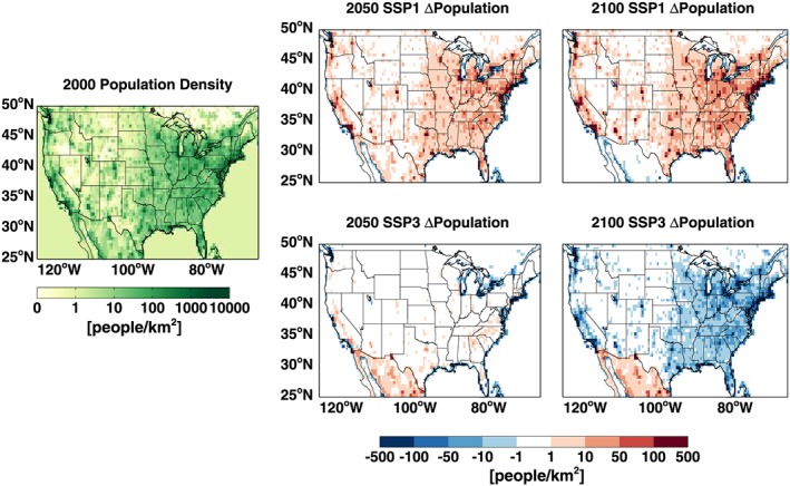
Figure shows the current CONUS population density (average 2006–2010) and the changes in population density projected in 2050 (average of 2040–2050) and 2100 (average of 2090–2100) by the SSP1 and SSP3 projections.

2.3. Visibility Calculations

We used the first IMPROVE equation (equation (2)) developed by Malm et al. (1994) to calculate potential changes in visibility. We chose to present results in the main text using the first equation rather than the revised equation (Pitchford et al., 2007) for better comparison with Val Martin et al. (2015). The revised equation also separates the organic mass into large and fine mode fractions using the total mass (if the total concentration is above 20 μg/m³, all of it is assumed to be in the large mode. If the concentration is below 20 μg/m³, then it is separated into small and large modes, which have different mass extinction efficiencies). Using this cutoff value based on total mass to distinguish between large and small modes created some counterintuitive results when examining our sensitivity simulation results on days with high concentrations. However, we did calculate these changes in visibility using the revised IMPROVE equation and found generally similar results (see section S5).

$$b_{\mathrm{ext}}\approx 3\times f\left(\mathrm{RH}\right)\times \left[\text{Ammonium Sulfate}\right]+3\times f\left(\mathrm{RH}\right)\times \left[\text{Ammonium Nitrate}\right]+4\times \left[\text{Organic Mass}\right]+10\times \left[\text{Elemental Carbon}\right]+1\times \left[\text{Fine Soil}\right]+0.6\times \left[\text{Coarse Mass}\right]+\text{Rayleigh scattering}$$ (2)

With the IMPROVE equation, light extinction (b _ext) at each IMPROVE site is calculated by multiplying the mass concentrations (in μg/m³) of different aerosol components by typical component‐specific mass extinction efficiencies. For sulfate and nitrate, the dry extinction efficiency is also multiplied by a water growth factor that is a function of relative humidity (f (RH)). Rayleigh scattering is assumed to be 10/Mm at every site, and gas absorption is assumed to be 0. For our results, we use the CESM ground‐level daily‐average relative humidity and daily‐average PM species concentrations.

We also convert this to a haze index (HI) following equation (3) (U.S. EPA, 2003) and visual range (VR) following equation (4) (Pitchford & Malm, 1994) as in Val Martin et al. (2015).

$$\mathrm{HI}=10*ln\left(b_{\mathrm{ext}}/10\right)$$ (3)

where b _ext is in inverse megameters.

$$\mathrm{VR}=K/b_{\mathrm{ext}}$$ (4)

where K is the Koschmieder coefficient and is assumed to be 3.91 in Pitchford and Malm (1994).

2.4. Health Impact

We calculate the all‐cause mortality associated with changes in the annual‐average concentrations in PM_2.5. We rely on the following concentration response function as used in Anenberg et al. (2010, 2014):

$$\mathrm{\Delta }\text{Mortality}=\mathrm{Pop}\left(1-{exp}^{-\beta *\mathrm{\Delta }X}\right)Y_0$$ (5)

In this equation, the change in mortality is determined by the population (Pop) and baseline mortality (Y ₀) and the concentration response function. The health response (here, mortality) is related to the change in annual‐mean PM_2.5 concentration (ΔX) using a concentration‐response factor or beta coefficient (β) determined from relative risk (RR) estimates in epidemiological studies. The β can be determined from the RR estimate following equation (6), which is commonly used (i.e., Anenberg et al., 2010, 2014; Fann et al., 2017) and assumes a linear relationship between the ambient concentration and the log of the RR. While some studies have suggested that a linear relationship would overpredict outcomes at high concentrations (Burnett et al., 2014; Nasari et al., 2016; Pope et al., 2015), this linearity has been demonstrated over the range of PM_2.5 values relevant to this study (Krewski et al., 2009).

$$\beta =ln\left(\mathrm{RR}\right)/\mathrm{\Delta }X$$ (6)

When calculating the ΔX for equation (5), studies often subtract the threshold value (concentration below which there is no effect) or use the original epidemiological studies lowest observed concentration. For this study, we use several different β coefficients commonly used in health impact assessments in order to determine a range of estimates for all‐cause mortality. To note, there are uncertainties not only in β but also in the application of the threshold/lowest‐observed‐concentration value, and shape of the concentration response function that will all impact our final estimates of the number of attributable premature deaths. We do investigate the impact of the threshold value for our estimates, but for a more‐detailed exploration and sensitivity analyses of these uncertainties on the estimates, see Johnston et al. (2012), Kodros et al. (2018), or Ford and Heald (2016).

In this study, we use β coefficients from Krewski et al. (2009), Crouse et al. (2012), and Laden et al. (2006). The RRs, confidence intervals (CIs), and threshold/lowest‐observed‐concentration values from these studies are given in Table 1. To note, all of these studies are of the health effects associated with total PM_2.5 mass. Therefore, by using these β coefficients for determining the burden contribution due only to smoke, we are assuming (as has been done in other studies) that all sources and aerosol types have equal toxicity, which may not be accurate. Recent review studies specific to wildfire smoke exposure (e.g., Liu et al., 2016; Reid et al., 2016) have highlighted both similar health effects to total PM_2.5 exposure studies (positive associations with respiratory morbidity) and some distinctions (no clear association with cardiovascular morbidity). However, while there have been many studies looking at the effects of acute exposure to wildfire smoke, there are no studies that have quantified the relationship between all‐cause mortality and long‐term exposure to smoke PM_2.5, which is what we are determining here. Therefore, previous studies (e.g., Johnston et al., 2012) have also relied on using RR values from studies of total PM_2.5 when estimating the number of premature deaths attributable to long‐term exposure to smoke PM_2.5.

Table 1.

Epidemiology Studies Used for Our Calculations of Attributable Premature Deaths With Their RRs, CIs, and Threshold/Lowest Observed Concentration Values

Study reference	Relative risk for ΔX = 10 μg/m3	Confidence interval	Lowest observed/threshold concentration
Krewski et al. (2009)	1.06	1.04–1.08	5.8 μg/m3
Crouse et al. (2012)	1.10	1.05–1.15	1.9 μg/m3
Laden et al. (2006)	1.16	1.07–1.26	10 μg/m3

For our final results, we use the Krewski et al. (2009) RR because it is widely used and derived from a large cohort population in the United States (American Cancer Society Cancer Prevention Study II). We pair the Krewski et al. (2009) RR with the lowest observable concentration from Crouse et al. (2012) because subsequent research since Krewski et al. (2009) has shown mortality effects of PM_2.5 exist at PM_2.5 concentrations below the minimum observed value of Krewski et al. (2009) of 5.8 μg/m³ (Crouse et al., 2012; Pinault et al., 2016). Other studies have assumed a threshold of 0 μg/m³ (i.e., Fann et al., 2017). We also examine the sensitivity to other choices in β coefficients and threshold values, and we present those results as well.

Population is taken from the SSP1 and SSP3 projections and is on a 0.5° spatial resolution grid. For baseline mortality, we use the SSP population death rate estimates for all‐cause mortality. These are given for five‐year time periods for each country. We use the nationally averaged death rate for the U.S. rate for each year in our simulation period, and we regrid the PM_2.5 concentrations to the same 0.5° resolution as the population to estimate exposure concentrations. There is a decrease in the mortality rates for SSP1 and an increase for SSP3.

Finally, to attribute the number of premature deaths to each source (nonfire, CONUS fire, and AK/HI/Mexico/Canadian transported smoke), we multiply the total number of premature deaths determined from the total PM_2.5 by the fraction of PM_2.5 from each source (determined from our sensitivity simulations). This method, as opposed to using the results from the sensitivity simulations with zeroed out emissions, avoids underestimating the contribution of sources that would occur given the dependence on the threshold value and the nonlinearity of the concentration response function (Kodros et al., 2018).

3. Results

3.1. Projections of Future Smoke Emissions in North America

From the CLM, the present‐day area burned for the CONUS (or Temperature North America, TENA) is 6.2 Mha/year (for 1995–2005); this is greater than the Global Fire Emissions Database version 4 (GFED4) estimate of 1.8 Mha/year (Giglio et al., 2013); however, this GFED4 estimate does not include small fires, which are important in the United States. The GFED4s estimate, which does include small fires, estimates an average of 2.7 Mha/year for 2001–2010 with a range of ~1.5–4 Mha/year (Randerson et al., 2012). The land model simulations described in section 2.1 showed an increase in area burned in the middle and late 21st century relative to the start of the century. As the burn area increases, biomass burning (BB) emissions also increase (whereas carbon emissions from other sources are projected to decrease). The total annual average emissions of BB BC and OC for the CONUS as determined from the CLM simulations are given in Table 2. Our early 21st century (2000) CONUS BB emissions of BC (0.058 Tg/year) are in the range of the GFED (0.011 Tg/year), Fire INventory National Center for Atmospheric Research (FINN; 0.024 Tg/year), and National Emissions Inventory (0.102 Tg/year) inventories as given in Larkin et al. (2014). Our CONUS OC BB emissions (0.84 Tg/year) are also between the Streets et al. (2004) estimate of 0.954 Tg/year (for 1996), the U.S. EPA (2006) estimate of 0.658 Tg/year (for 2000), and FINNv1 estimate of 0.405 Tg/year (Wiedinmyer et al., 2011). Results from the CLM interactive fire simulations shown in Table 2 suggest that emissions should double by midcentury in the RCP4.5 (increase by ~50% in RCP8.5) and almost triple by 2100 in RCP8.5. As noted in Val Martin et al. (2015), the standard RCP4.5, which does not include prognostic future fire emissions from CLM (as done here) or a statistical fire prediction model (e.g., Yue et al., 2013), suggests an increase of about 60% in fire OC emissions over the western United States by 2050 while the RCP8.5 suggests a 0.3% decrease in these emissions. These assume that fire emission changes are because the standard RCP scenarios consider land use changes (afforestation in RCP4.5 and deforestation with a transition to more croplands in RCP8.5), but not any climate effects (Lamarque et al., 2010; Val Martin et al., 2015). Using a statistical fire model that did include climate changes on fires (and relied on output from 15 climate models using the A1B scenario), Yue et al. (2013) predicted a 150–170% increase in OC and BC fire emissions in the western United States by 2050. Thus, by adding in an increase in fire emissions following Yue et al. (2013), Val Martin et al. (2015) had similar increases in emissions in the western United States as shown here (~100% in RCP4.5 and ~50% in RCP8.5 increase by 2050).

Table 2.

Decadal‐Average Black Carbon and Organic Carbon Emissions in the Contiguous United States Due to Biomass Burning

	2000–2010	2040–2050		2090–2100
CONUS biomass burning emissions	Baseline	RCP4.5	RCP8.5	RCP4.5	RCP8.5
Black carbon (Tg year)	0.058	0.13	0.087	0.12	0.14
Organic carbon (Tg year)	0.84	1.9	1.3	1.9	2.1

However, we find significant spatial differences in where the changes in BB emissions occur compared to these previous studies. In Figure 2, we show the early 21st century (average 2000–2010) BC and OC BB emissions over the CONUS and the changes for 2050 (annual average for 2040–2050) and 2100 (average 2090–2099) for the RCP4.5 and RCP8.5 scenarios determined from the land model simulations. The largest projected changes are in the southeastern United States and along the Canadian border (Figure 2). These increases in BB emissions in the eastern United States are an important distinction of this current work, as previous studies such as Yue et al. (2013) and consequently Val Martin et al. (2015) did not consider any significant increases in area burned or fire emissions over the eastern United States and only focused on the western United States. Yue et al. (2013) predicted a 150–170% increase in fire‐related OC and BC emissions in the western United States by midcentury using the A1B scenario. Here we find a 60% (RCP8.5) or 130% (RCP4.5) increase for the whole United States in midcentury; however, the majority of the increase in BC + OC emissions is for the eastern United States (85% RCP8.5, 220% RCP4.5) and not the western United States (40% RCP8.5, 45% RCP4.5). Like Yue et al. (2013), our simulations show that the western United States has peak fire emissions in August throughout the century. Additionally, the northeastern United States has a similar fire season compared to the western United States, whereas the southeastern United States has peak fire emissions earlier in May. For all regions, the annual fire emissions increase due to both increases in emissions during the peak fire season and a lengthening of the fire season, with the largest changes in both the peak emissions and lengthening occurring in the southeastern United States.

Figure 2.

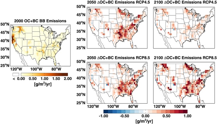
Early 21st century (2000), decadal average OC and BC BB emissions for the CONUS, and the changes for 2040–2050 and 2090–2100 projected with the RCP4.5 and RCP8.5 scenarios.

In the CLM simulations (Pierce et al., 2017), both climate and population changes drive the fire emissions. In both the RCP4.5 and RCP8.5 scenarios, the relevant climate changes (i.e., temperature, precipitation, and soil moisture) throughout the United States are overall conducive to increasing fire emissions in the future (Stocker et al., 2013; Val Martin et al., 2015, Figure S1), and climate is the main driver of our simulated changes in fire emissions in the CONUS (Pierce et al., 2017, Figure S2). The RCP4.5 scenario projects strong afforestation up to 2050 over the southeastern United States due to mitigation strategies for carbon emission reductions (shown in Val Martin et al., 2015); this rate begins to stabilize after 2050, and there is less fuel recovery by 2100. While climate is the primary driver of fire changes in the United States, population changes also impact fires, particularly the suppression and ignition of fires. The SSP1 (used with RCP4.5) projects an increase in population over the CONUS (Figure 1), which leads to increased suppression of fires in the eastern United States in the CLM, offsetting some of the increases in fires that might be projected if only changes in climate are considered (Val Martin et al., 2015). The RCP8.5 scenario projects deforestation in much of the eastern United States and a transition to more croplands leading to less fuel available to burn. Correspondingly, the RCP8.5 scenario does suggest a slight increase in agricultural burning in the southeast (although landscape fires overall dominate the area burned). Additionally, the SSP3 (used with RCP8.5) projects little population change by 2050 and then widespread decreases by 2100 (Figure 1). This leads to less suppression of fires, which coupled with the changes in climate, increases fire emissions significantly between the midcentury and late century.

Because our model simulations suggest that BB in the eastern United States could significantly increase, and as population and PM_2.5 concentrations are generally higher in the eastern United States compared to the western United States (with the exception of California), this could have important implications for smoke exposure and the resulting health effects.

3.2. Projections of Future PM and Fire PM in the United States

Changes in emissions will also alter PM_2.5 concentrations levels in the CONUS. By 2050, total PM_2.5 concentrations are projected to decrease primarily due to expected reductions in anthropogenic emissions in both the RCP4.5 and RCP8.5 scenarios (Figure 3). The reductions shown here are most notable in the eastern United States, particularly in the Ohio River Valley, consistent with recently observed downward trends in this region (e.g., Malm et al., 2017; U.S. EPA, 2012). In our RCP4.5 scenario simulations, PM_2.5 concentrations will continue to decrease by 2100; however, in the RCP8.5 scenario, several areas in the western United States, northeastern United States, and southeastern United States are projected to have higher concentrations compared to the early 21st century (2000). Our results shown here in Figure 3 differ from Lam et al. (2011), which showed that PM_2.5 should decrease drastically by 2050. However, they did not account for changing fire emissions.

Figure 3.

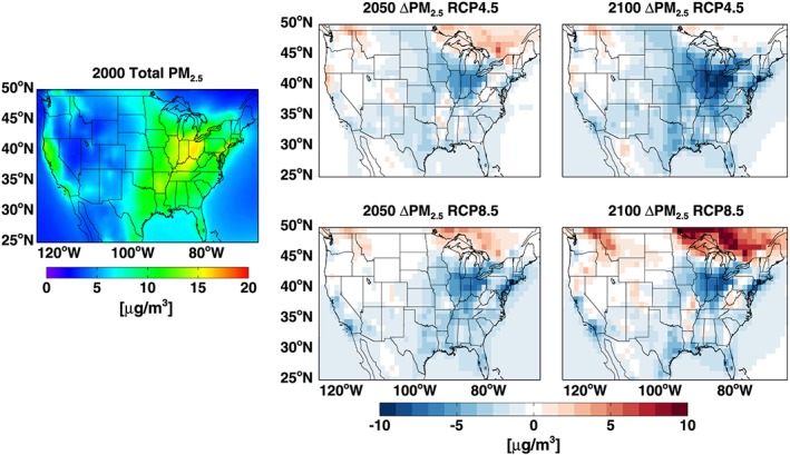
Total surface PM_2.5 concentrations in the CONUS for early 21st century, and the projected change (compared to early 21st century) in surface PM_2.5 concentrations by midcentury and late century from the baseline CESM simulations using the RCP4.5 and RCP8.5 scenarios.

In Figure 4, we show the decadal average of the annual changes in fire‐related PM_2.5 projected in our simulations (summertime [June‐July‐August] average is shown in Figure S6). These results indicate that smoke concentrations are the cause for the higher PM_2.5 in our future simulations and that without an increased contribution from smoke, many regions would be projected to have even lower PM_2.5 concentrations than shown in Figure 3. Both our RCP4.5 and RCP8.5 scenarios suggest that PM_2.5 due to fire emissions will increase in the future. There are three main regions that will be impacted: (1) the Pacific Northwest (and northern California), (2) the southeastern United States, and (3) the north‐central and northeastern United States along the Canadian border. In the early 21st century, fire emission accounts for more than 50% of the annual PM_2.5 only in the Pacific Northwest (Figure S6). By 2100 in both our RCP4.5 and RCP8.5 scenarios, fire emissions are projected to account for more than 50% of the annual PM_2.5 across most of the CONUS, and in areas of the three previously mentioned regions, fire emissions are projected to be responsible for 75% or more of the annual average PM_2.5 concentrations in the RCP8.5 scenario (Figure S7).

Figure 4.

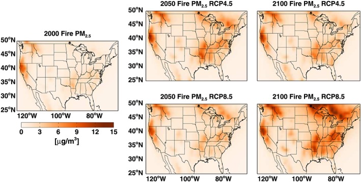
Simulated decadal average PM_2.5 concentrations due to fire emissions from the land model in 2000 and as projected in 2050 and 2100 in the RCP4.5 and RCP8.5 simulations (with the land model fire emissions).

Figure 5 shows the average PM_2.5 concentrations divided by species over the CONUS from our simulations. Inorganic species (sulfate and nitrate ammonium) are predicted to decrease, while SOA and OA concentrations will increase. SOA is predicted to increase with increasing biogenic emissions as shown in Val Martin et al. (2015), while the OA increase is primarily due to fire emissions, as BB is the largest emission source of OC in the United States. Although Val Martin et al. (2015) used different fire emissions (scaled RCP4.5 and RCP8.5 scenario fire emissions to match Yue et al., 2013), they also showed that OA concentrations would double by 2050 due to fire emissions in both the RCP4.5 and RCP8.5 scenarios. BC is predicted to decrease as mobile and industrial emissions are significant but decreasing sources, and BB is not currently the major source of BC in the United States. Yue et al. (2013) found that wildfire emissions increased western U.S. summertime OC by 46–70% and BC by 20–27% at midcentury compared to the present day. Here we find that if we do not consider changes in anthropogenic emissions, wildfire emissions would lead to a 16% (28%) increase in summertime BC averaged for the CONUS and a 51% (86%) increase in OA in the RCP8.5 (4.5) scenario by midcentury.

Figure 5.

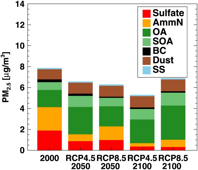
Average (decadal means) PM_2.5 concentrations over the CONUS separated by species for early 21st century, midcentury, and late century from the RCP4.5 and RCP8.5 scenarios.

Because of the large concentration increases along the border in the Northeast as shown in Figures 3 and 4 (where there are large population centers) projected in the RCP8.5 scenario, we also wanted to determine how much of this increase could be due to smoke transported from North American regions outside CONUS. Figure 6 shows the results from our TransportFireOff simulation (where fire emissions in Canada, Alaska, and Hawaii were turned off), which suggests that not only will concentrations increase due to local fires but also fire emissions in Canada could cause a 1–5 μg/m³ increase in PM_2.5 in the RCP8.5 scenario (absolute concentrations are shown in Figure S8). This is approximately 50% of the smoke PM_2.5 in the northern United States, which suggests that smoke from Alaskan or Canadian fires could be responsible for 25% of the annual PM_2.5 burden in the northern United States by 2100 compared to 5% in the early 21st century.

Figure 6.

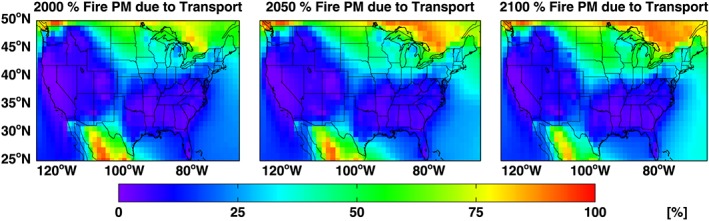
Percent of smoke PM_2.5 due to transport (fires outside the CONUS) for 2000 and in 2050 and 2100 with the RCP8.5 scenario.

For the CONUS‐wide decadal average, the fire‐related contribution to PM_2.5 concentrations is projected to go from ~25% to over 50% by 2100 in both the RCP4.5 and RCP8.5 scenarios (Figure 7; regional results are shown in Figure S9). In the RCP8.5 scenario, smoke will almost completely offset the projected reductions in nonfire PM_2.5 from the early 21st century. To note, this is for the (decadal) annual averages. During the fire season, the concentrations (and thus, the exposure concentration levels) will be even higher. In the southeast, midsouth, northeast, and west regions the summertime (June, July, and August) average in our simulations (see Figure S10) is above the World Health Organization (WHO) guideline of 10 μg/m³ and the EPA national ambient air quality standard limit of 12 μg/m³ (these standards/guidelines are for annual averages).

Figure 7.

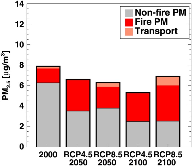
Decadal average PM_2.5 concentrations over the CONUS separated by source (nonfire, fire, and AK/HI/Mexico/Canadian transported smoke from fires) for early 21st century, midcentury, and late century from the RCP4.5 and RCP8.5 scenarios (simulations to determine transported smoke were only conducted for RCP8.5 scenario).

3.3. Projections of Visibility Changes in the United States

The Regional Haze Program was established with the goal of reducing visibility impairment in National Parks, forests, and historic sites around the United States. According to our simulations, visibility will increase in many of these designated areas in the eastern United States due to decreases in anthropogenic emissions. However, in the western United States where concentrations are predicted to increase due to wildland fire smoke, visibility could worsen by 2100. Additionally, wildfires are not a continuous emission source; their timing and location are sporadic, and they can produce large emission spikes on day to week timescales. Therefore, while the impact on the annual timescale may be relatively small, the contribution to a single day could be quite large. The Regional Haze Rule requires states to set goals to improve visibility and reach natural conditions on both the clearest (average of bottom 20% over 5‐year period) and haziest (average of bottom 20% over 5‐year period) days by 2064.

In these RCP8.5 simulations (for RCP4.5 results, see Figure S3, and for results with revised equation, see Figure S4), we see that the 20% best days are projected in our simulations to have improved visibility by 2050 and 2100 (Figure 8). However, when we look at the 20% worst days, our simulation results suggest that smoke from fires would lead to visibility degradation in many regions of western United States and the southeastern United States in 2050, which would then worsen by 2100 (Figure 8). Particular areas of vulnerability include parks in the western United States (e.g., Glacier National Park, Lassen Volcanic National Park), southeastern United States (e.g., Great Smoky Mountains National Park), and in the northeastern United States (e.g., Acadia National Park). If we compare to results from our FireOff simulation, we see that this is due to fires. Without fires, our projections suggest that visibility would continue to improve by 2050 and 2100. Visibility projections from our RCP4.5 simulations suggest similar spatial changes (visibility degradation on the worst days in the west and southeastern United States), but with different magnitudes. These results differ from the projections shown in Val Martin et al. (2015), which showed that visibility would improve on the worst and best days by 2050 in both the RCP4.5 and RCP8.5 scenarios. As we are using the same anthropogenic emissions as Val Martin et al. (2015), these differences are due to the CLM‐predicted fire emissions, which have a different magnitude and spatial distribution of changes during the 21st century. As mentioned in section 3.1, Val Martin et al. (2015) only considered fire emission changes in the western United States, whereas the simulations used in this study suggest much larger changes in the eastern United States.

Figure 8.

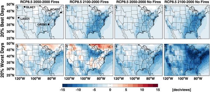
Change in the haze index calculated for the average of the (top row) 20% best and (bottom row) 20% worst days by 2050 and 2100 in the RCP8.5 scenario determined from our baseline simulation (“fires”) and our FireOff simulation (“no fires”). Sites in Figure 9 are labeled as follows: Acadia National Park in ME (ACAD1), Great Smoky Mountains National Park in TN (GRSM1), and Lassen Volcanic National Park in northern CA (LAVO1).

In Figure 9 (Figure S4 for revised equation), we show the cumulative probability distributions of the HI at four different national park locations in the United States that will potentially experience more visibility degradation due to fires: Acadia National Park in ME (ACAD1), Glacier National Park in MT (GLAC1), Great Smoky Mountains National Park in Tennessee Mountains (GRSM1), and Lassen Volcanic National Park in northern CA (LAVO1). In general, our simulations suggest that visibility should improve in the future on the average day and on the cleanest days. At the northeastern (ACAD1) and southeastern (GRSM1) sites, fire‐related PM has little impact on visibility in the early 21st century (little difference between the fire and no fire results). At the western sites, and particularly at the northern California site (LAVO1), fire‐related PM has a larger impact on visibility, especially on the days with the worst visibility. For all sites, fire‐related PM_2.5 will play a larger part in visibility degradation in 2050 and 2100 (in the RCP8.5 scenario) and more days will be impacted by fire‐related PM compared to the early 21st century. In Figure 9, we also have the 2,064 HI targets marked for each state. Our simulation results suggest that for the four sites shown here, that smoke will make it difficult to reach the haziest day targets. Without smoke, all of the sites would be able to reach both the haziest day and clearest day targets (by 2100); with smoke, only ACAD1 will reach the clearest day goal. However, these simulation results may not be completely representative of the necessary rate of progress needed to reach the goals as we have not analyzed how well our simulations match the real baseline conditions (determined from 2000 to 2004) at each site.

Figure 9.

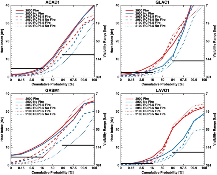
Cumulative probability distributions of the haze index (equation (3)) and visibility range (equation (4)) at Acadia National Park in ME (ACAD1), Great Smoky Mountains National Park in TN (GRSM1), and Lassen Volcanic National Park in northern CA (LAVO1) for our different RCP8.5 model simulations and time periods. The solid black lines show the 2064 HI targets for the clearest (average of bottom 20%) and haziest (average of top 20%) days at each site. Location of sites is noted in Figure 8.

3.4. Projections of Population‐Level PM Exposure in the United States

While emissions and concentrations are expected to change, population is also expected to change in the future. This population change will impact the population‐level exposure and the expected health effects. Thus, it is important to determine not only the average concentration but also the average exposure concentration experienced by populations in different regions.

In Figure 10, we calculate the population‐weighted average concentrations for the different regions of the United States (same regions as in Val Martin et al., 2015). Both the RCP8.5 and RCP4.5 scenarios predict a decrease in the decadal average of the annual population‐weighted PM_2.5 by 2050, suggesting that population‐level exposure will improve for all regions of the United States. This is due both to decreasing urban emissions and population changes. However, in several regions (such as the Great Plains and Southwest), increases in fire PM_2.5 will offset a significant amount of the improvements in exposure levels associated with decreases in anthropogenic emissions. Additionally, in every region, our simulations suggest that smoke will become a dominant source of the annual average PM_2.5 exposure, even in regions that are not typically associated with wildfires, such as the Northeast and Midsouth. In these two regions, much of this increase is due to transport of smoke from other regions.

Figure 10.

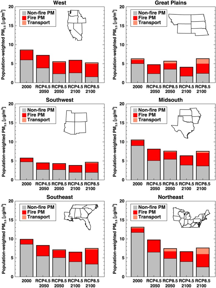
Decadal average of the annual population‐weighted PM_2.5 concentrations for different regions of the CONUS (as defined in Val Martin et al., 2015) separated by source (nonfire, fire, and transported smoke from fires) for early 21st century (2000), midcentury (2050), and late century (2100) from the RCP4.5 and RCP8.5 scenarios (simulations to determine transported smoke were only conducted for the early 21st century and RCP8.5 projection scenarios).

In our RCP8.5 scenario simulations, population‐level exposure concentrations in most regions is projected to increase or stay consistent in 2100 compared to 2050 due to increasing fire emissions offsetting decreasing nonfire emissions. For the Great Plains and Northeast, transported smoke from Canada is a significant part of this projected increase (we did not do transport sensitivity simulations for the RCP4.5 scenario).

3.5. Projections of the Health Impact of PM_2.5 and Fire PM_2.5 in the CONUS

From the PM_2.5 concentrations and population estimates, we determine the burden on premature deaths attributable to PM_2.5 exposure following the method outlined in section 2.3. In Table 3, we show results acquired using different RRs and threshold values from the studies described in the methods (Table 1). Laden et al. (2006) calculated a higher RR, but also had a higher lowest observed level, such that using this value as the threshold value causes concentrations for much of the United States to fall below this value and not contribute to the number of premature deaths attributable to PM_2.5. The highest estimates come from using the Crouse et al. (2013) RR and threshold value. The range of estimates shown here highlights the importance of the assumptions that are used in determining the health impact. Including results using these different assumptions can make our results more comparable to other studies that use different baseline assumptions.

Table 3.

Number (1000s) and Percent (in Parentheses) of Premature Deaths Attributable to Total PM_2.5 Exposure per Year Determined From Using Different RRs and Threshold/Lowest Observed Values for the Different Time Periods and RCP Scenarios

	2000	2050		2100
Study for RR; threshold value used	Baseline	RCP4.5	RCP8.5	RCP4.5	RCP8.5
Krewski et al., 2009; X 0 = 0.0 μg/m3	167 (6.1%)	147 (4.8%)	145 (3.9%)	107 (3.6%)	121 (3.9%)
Krewski et al., 2009; X 0 = 1.9 μg/m3 a	138 (5.1%)	114 (3.7%)	105 (2.9%)	75 (2.5%)	88 (2.9%)
Krewski et al., 2009; X 0 = 5.8 μg/m3	80 (2.9%)	50 (1.6%)	31 (0.84%)	17 (0.57%)	30 (0.99%)
Crouse et al., 2012; X 0 = 1.9 μg/m3	222 (8.1%)	185 (6.0%)	171 (4.6%)	121 (4.1%)	142 (4.7%)
Laden et al., 2006; X 0 = 10.0 μg/m3	69 (2.5%)	28 (0.91%)	6 (0.17%)	5 (0.17%)	16 (0.53%)

^aStudy and threshold value used for results shown in Figure 11.

To determine the source‐specific contribution from fires, we multiplied the total premature deaths by the fraction of PM_2.5 from each source in each grid. Results are shown in Table 4 (which provides the range of estimates using the different RRs and threshold values). Both our RCP4.5 and RCP8.5 scenario simulations suggest that the number of premature deaths attributable to fire‐related PM_2.5 will increase in 2050. In our simulations with the RCP4.5 scenario, it is projected that the number of attributable deaths will decrease by 2100 (but still be higher than in the early 21st century), while the number of premature deaths attributable to fire‐related PM_2.5 is projected to continue to rise by 2100 in our RCP8.5 scenario simulation.

Table 4.

Number (1000s) and Percent (in Parentheses) of Premature Deaths Attributable to Fire PM_2.5 Exposure Determined From Using Different RRs and Threshold/Lowest Observed Values for the Different Time Periods and RCP Scenarios

	2000	2050		2100
Study for RR; threshold value used	Baseline	RCP4.5	RCP8.5	RCP4.5	RCP8.5
Krewski et al., 2009; X 0 = 0.0 μg/m3	21 (0.89%)	53 (1.7%)	43 (1.4%)	45 (1.5%)	59 (2.4%)
Krewski et al., 2009; X 0 = 1.9 μg/m3 a	17 (0.70%)	42 (1.4%)	32 (1.0%)	32 (1.1%)	44 (1.8%)
Krewski et al., 2009; X 0 = 5.8 μg/m3	10 (0.4%)	20 (0.66%)	11 (0.34%)	9 (0.31%)	18 (0.70%)
Crouse et al., 2012; X 0 = 1.9 μg/m3	28 (1.2%)	67 (2.2%)	51 (1.7%)	52 (1.8%)	71 (2.9%)
Laden et al., 2006; X 0 = 10.0 μg/m3	7 (0.31%)	15 (0.49%)	3 (0.09%)	4 (0.13%)	11 (0.41%)

^aStudy and threshold value used for results shown in Figure 11.

We summarize these results in Figure 11, which shows the calculated annual number (Figure 11a) and percentage (Figure 11b) of premature deaths attributable to PM_2.5 exposure in the CONUS using model‐simulated PM_2.5 concentrations, the SSP population projections, the projected U.S. mortality rates from the SSPs, the concentration‐response function (equations (5) and (6)), the Krewski et al. (2009) RR listed in Table 1, and the threshold value from Crouse et al. (2013) listed in Table 1 (regional estimates are given in the Figures S11 and S12). Our results using these baseline assumptions suggest that approximately 5% of the total deaths in the CONUS are attributable to PM_2.5 in the early 21st century (range of 2‐*% with different assumptions), which is in the range estimated by several previous studies (roughly 2–11% in Fann et al., 2012; Ford & Heald, 2016; Lim et al., 2012; Punger & West, 2013; and Sun et al., 2015). Estimates from our model simulations suggest that the overall number of premature deaths attributable to PM_2.5 should decrease in the United States in both the RCP4.5 and RCP8.5 scenarios. However, the U.S. population also changes throughout the century as well as the baseline mortality rates. In the SSP1 scenario (used with RCP4.5), population increases, while in the SSP3 scenario (used with RCP8.5), population declines; thus, the percent of premature deaths attributable to PM_2.5 is projected to remain at 3–4% of the total deaths. We also find (using the baseline assumptions) that 0.70% of total deaths (12.5% of the premature deaths attributable to total PM_2.5) are due to fire‐related PM_2.5 in the early 21st century. The percent of deaths attributable to fire‐related PM_2.5 increases by the end of the 21st century to 1.1% and 1.8% for our respective RCP4.5 and RCP8.5 cases. While the overall trends in mortality number and percent are similar in both panels of Figure 11, the qualitative differences between the two panels are due to changing population and baseline mortality rates in the future.

Figure 11.

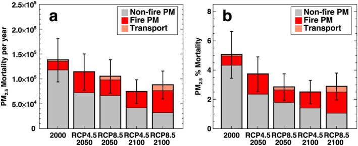
(a) Number and (b) percent of premature deaths attributable to PM_2.5 per year in 2000, 2050, and 2100 following the RCP4.5 and RCP8.5 scenarios and separated by source (nonfire, fire, and transported smoke). The black lines show the estimate range for the total attributable deaths from the RR CIs.

4. Discussion of Uncertainties

We have presented here estimates of future (2050 and 2100) air quality, health effects, and visibility in the CONUS determined from CESM simulations using emissions from a prognostic fire model. These are predictions and the veracity of the results will be limited by the model and the assumptions we made to calculate visibility and the health effects. These model simulations are uncertain due to the nature of the study which relies on RCP emission scenarios and SSPs. We are only using a single model and single simulations for each scenario. Compared to other models, CAM is more sensitive to CO₂ forcings and therefore produces stronger climate changes (Meehl et al., 2013). However, climate studies have shown that projections of decadal‐mean temperatures at the end of the 21st century for specific global regions can vary greatly between simulations of even a single model due to internal variability in large‐scale oceanic and atmospheric dynamics (e.g., Deser et al., 2012). Hence, we expect that an ensemble of CESM simulations would provide a range of potential future smoke PM_2.5 concentrations and associated visibility and health effects. However, due to the computational complexity of the CAM‐Chem simulations at the simulated resolution, we were only able to perform one set of simulations. Future work should consider ensembles of simulations.

Additionally, the model is limited by the processes that it is able to represent. While this study does use wildfire emission estimates that were calculated with a land model (unlike many previous studies), the land model was not run dynamically/online in the CESM simulation of atmospheric concentrations. Therefore, there are potential land‐atmosphere interactions that are not represented. Additionally, while the model was run at a relatively fine global resolution for a global chemistry‐climate model, the grid spacing (~100 km) does not capture some important variability in concentrations relevant to the United States. At this resolution, model simulations tend to smooth out concentrations over broad regions and therefore cannot predict the high exposure concentrations often associated with dense smoke plumes or urban centers.

Not only are there large uncertainties in the PM_2.5 concentrations, but we are also limited in calculating the health burden by using the simple formulation give in equation (2). While this method is often used to provide estimates of the attributable premature deaths, studies can use different RR values, threshold values, and different formulations, or apply it to different resolutions of exposure estimates (i.e., grid level or country level), that can all lead to large uncertainties in the final numbers. A few examples were given in Table 1, but there is a large range in the RRs found in different epidemiology studies (see Ford & Heald, 2016). Additionally, we are assuming that the association between mortality and PM_2.5 remains constant over the study time period, irrespective of change in composition (we assume all PM_2.5 has the same toxicity), health care access, population activity, or other factors that might modify the relationship over time. The SSP1 and SSP3 population and mortality estimates are also model predictions that rely on many assumptions.

While there are the uncertainties described above, our results do suggest that wildfire smoke will account for a large amount of the premature deaths associated with PM exposure in the future and could offset many of the health gains from reducing anthropogenic emissions, especially by the year 2100. Future work should include ensembles of simulations and combinations of coupled land‐fire‐atmospheric models with statistical fire projections to quantitatively map the range of uncertainties in future projections.

5. Conclusion

This study used CESM simulations of the early 21st century, midcentury, and late century surface PM_2.5 to determine the potential impact of fires on visibility, exposure, and mortality in the CONUS. Unlike previous studies, these simulations used burn area determined from a land and fire model, which includes not only climate changes but also socioeconomic drivers. We looked at two scenarios for the future: the RCP4.5 scenario with SSP1 and the RCP8.5 scenario with SSP3 to provide the first estimates of future smoke visibility and health impacts from model simulations using emissions determined from a prognostic fire model.

Here we show, as other studies (e.g., Spracklen et al., 2009; Yue et al., 2013) have shown, that wildfire emissions will likely increase in the United States in the middle and late 21st century, while U.S. anthropogenic emissions will continue to decrease. However, unlike previous studies that focused on the western United States, our simulations suggest that there will also be significant increases in fire emissions in the southeastern United States. Our unique result could also be due to including population changes and assumptions about afforestation and deforestation in our simulations as discussed in section 3.1. Additionally, these previous studies mainly relied on parameterizations determined from statistical regressions of current day conditions while we are using a land fire model, which could explain these discrepancies. Therefore, while we are only presenting one set of simulations, these differing results do suggest that more work needs to be done using models that better account for feedbacks between climate, land use, and emissions to understand how the statistical relationships between these variables might change under different scenarios to alter fire regimes.

In many regions, the decrease in anthropogenic emissions will lead to a decrease in PM_2.5 concentrations, visibility, population‐level exposure, and associated premature deaths. However, in some regions of the United States, the potential improvements will be partially offset by increases in wildfire emissions. Results from the CLM suggest that BC and OC emissions from fires will double with the largest changes in the western United States, along the Canadian border, and in the southeastern United States. By 2100, both the RCP4.5 and RCP8.5 scenarios suggest that fire‐related PM will account for more than 50% of the annual average PM_2.5 concentration in the CONUS. This will be due to both local fires and transported smoke. Smoke transported from outside the CONUS (AK/HI/Mexico/Canada) could account for >50% of the fire‐related PM in the Great Plains and Northeast regions in the RCP8.5 scenario.

Most of our results are for the decadal average, but wildfire smoke tends to be seasonal with large daily variability. Therefore, when looking at visibility, we saw that while the average visibility will improve, the visibility on the worst days could get even worse, particularly in the western United States, southeastern United States, and northeastern United States. We project that wildfire smoke will be the main cause of visibility degradation on the worst days in these regions.

Previous studies have quantitatively determined relationships between PM_2.5 exposure and premature deaths. Using these relationships, we calculated the burden for the early 21st century and future scenarios. We found that approximately 138,000 deaths (5.1% of total deaths) are attributable to total PM_2.5 in the early 21st century with 17,000 (0.7%) of these deaths attributable to fire‐related PM_2.5. The number of total deaths attributable to PM_2.5 is projected to decrease in both scenarios over the next century, but the number attributable to fire‐related PM will increase to 42,000 (1.4%, RCP4.5) or 32,000 (1.0%, RCP8.5) by 2050 and 32,000 (1.1%, RCP4.5) or 44,000 (1.8%, RCP8.5) by 2100.

Fires are potentially less controllable than urban and anthropogenic emission sources, and although there has been increased efforts to better manage fuels and forests in the United States to reduce wildfire risk, the number and intensity of wildfires has continued to increase. This is in large part due to the fact that fire frequency and intensity are strongly linked to the climate. While it is difficult to confidently determine how much the health burden could be reduced under a future climate with an RCP4.5 scenario compared to an RCP8.5 scenario (and decoupled from the changes in population) from our limited set of simulations, mitigation of climate change that could lead to a less warm and dry future climate should reduce the potential fire risks. In our simulations, we also saw that population changes had an impact on our exposure and mortality estimates, and more people are currently moving into the wildland‐urban interface in the western United States, leading to a greater risk of wildfire smoke exposure. Additionally, both the RCP4.5 and RCP8.5 scenarios suggested that while the overall PM_2.5 health burden would decrease, the fraction attributable to smoke exposure could increase in the future. Therefore, to continue to reduce the health burden associated with PM_2.5 in the CONUS, more emphasis will need to be put on reducing fire‐related PM exposure through public health campaigns (installing filters, creating clean air shelters, etc.) in conjunction with climate mitigation efforts.

Supporting information

Supporting Information S1

Ford, B. , Val Martin, M. , Zelasky, S. E. , Fischer, E. V. , Anenberg, S. C. , Heald, C. L. , & Pierce, J. R. (2018). Future fire impacts on smoke concentrations, visibility, and health in the contiguous United States. GeoHealth, 2, 229–247. 10.1029/2018GH000144

References

- Anenberg, S. C. , Horowitz, L. W. , Tong, D. Q. , & West, J. J. (2010). An estimate of the global burden of anthropogenic ozone and fine particulate matter on premature human mortality using atmospheric modeling. Environmental Health Perspectives, 118(9), 1189–1195. 10.1289/ehp.0901220 [DOI] [PMC free article] [PubMed] [Google Scholar]
- Anenberg, S. C. , West, J. J. , Yu, H. , Chin, M. , Schulz, M. , Bergmann, D. , et al. (2014). Impacts of intercontinental transport of anthropogenic fine particulate matter on human mortality. Air Quality, Atmosphere and Health, 7(3), 369–379. 10.1007/s11869-014-0248-9 [DOI] [Google Scholar]
- Balch, J. K. , Bradley, B. A. , Abatzoglou, J. T. , Nagy, R. C. , Fusco, E. J. , & Mahood, A. L. (2017). Human‐started wildfires expand the fire niche across the United States. Proceedings of the National Academy of Sciences, 114(11), 2946–2951. 10.1073/pnas.1617394114 [DOI] [PMC free article] [PubMed] [Google Scholar]
- Burnett, R. T. , Pope, C. A. III , Ezzati, M. , Olives, C. , Lim, S. S. , Mehta, S. , et al. (2014). An integrated risk function for estimating the global burden of disease attributable to ambient fine particulate matter exposure. Environmental Health Perspectives. 10.1289/ehp.1307049 [DOI] [PMC free article] [PubMed] [Google Scholar]
- Crouse, D. L. , Peters, P. A. , van Donkelaar, A. , Goldberg, M. S. , Villeneuve, P. J. , Brion, O. , et al. (2012). Risk of nonaccidental and cardiovascular mortality in relation to long‐term exposure to low concentrations of fine particulate matter: A Canadian National‐Level Cohort Study. Environmental Health Perspectives, 120(5), 708–714. 10.1289/ehp.1104049 [DOI] [PMC free article] [PubMed] [Google Scholar]
- Deser, C. , Phillips, A. , Bourdette, V. , & Teng, H. (2012). Uncertainty in climate change projections: The role of internal variability. Climate Dynamics, 38(3–4), 527–546. 10.1007/s00382-010-0977-x [DOI] [Google Scholar]
- Fann, N. , Kim, S.‐Y. , Olives, C. , & Sheppard, L. (2017). Estimated changes in life expectancy and adult mortality resulting from declining PM2.5 exposures in the contiguous United States: 1980‐2010. Environmental Health Perspectives, 125(9), 97003 10.1289/EHP507 [DOI] [PMC free article] [PubMed] [Google Scholar]
- Fann, N. , Lamson, A. D. , Anenberg, S. C. , Wesson, K. , Risley, D. , & Hubbell, B. J. (2012). Estimating the National Public Health Burden associated with exposure to ambient PM2.5 and ozone. Risk Analysis, 32(1), 81–95. 10.1111/j.1539-6924.2011.01630.x [DOI] [PubMed] [Google Scholar]
- Ford, B. , & Heald, C. L. (2016). Exploring the uncertainty associated with satellite‐based estimates of premature mortality due to exposure to fine particulate matter. Atmospheric Chemistry and Physics, 16(5), 3499–3523. 10.5194/acp-16-3499-2016 [DOI] [PMC free article] [PubMed] [Google Scholar]
- Fusco, E. J. , Abatzoglou Balch, J. K. , Finn, J. T. , & Bradley, B. A. (2016). Quantifying the human influence on fire ignition across the western USA. Ecological Applications, 26(8), 2390–2401. 10.1002/eap.1395 [DOI] [PubMed] [Google Scholar]
- Giglio, L. , Randerson, J. T. , & van der Werf, G. R. (2013). Analysis of daily, monthly, and annual burned area using the fourth‐generation global fire emissions database (GFED4). Journal of Geophysical Research: Biogeosciences, 118, 317–328. 10.1002/jgrg.20042 [DOI] [Google Scholar]
- Guenther, A. B. , Jiang, X. , Heald, C. L. , Sakulyanontvittaya, T. , Duhl, T. , Emmons, L. K. , & Wang, X. (2012). The Model of Emissions of Gases and Aerosols from Nature version 2.1 (MEGAN2.1): an extended and updated framework for modeling biogenic emissions. Geoscientific Model Development, 5, 1471–1492. 10.5194/gmd-5-1471-2012 [DOI] [Google Scholar]
- Hand, J. L. , Schichtel, B. A. , Malm, W. C. , & Frank, N. H. (2013). Spatial and temporal trends in PM2.5 organic and elemental carbon across the United States [research article]. Retrieved March 14, 2018, from https://www.hindawi.com/journals/amete/2013/367674/
- Hand, J. L. , Schichtel, B. A. , Pitchford, M. , Malm, W. C. , & Frank, N. H. (2012). Seasonal composition of remote and urban fine particulate matter in the United States. Journal of Geophysical Research, 117, D05209 10.1029/2011JD017122 [DOI] [Google Scholar]
- Johnston, F. H. , Henderson, S. B. , Chen, Y. , Randerson, J. T. , Marlier, M. , DeFries, R. S. , et al. (2012). Estimated global mortality attributable to smoke from landscape fires. Environmental Health Perspectives, 120(5), 695–701. 10.1289/ehp.1104422 [DOI] [PMC free article] [PubMed] [Google Scholar]
- Jones, B. , & O'Neill, B. C. (2016). Spatially explicit global population scenarios consistent with the shared socioeconomic pathways. Environmental Research Letters, 11(8), 10 10.1088/1748-9326/11/8/084003 [DOI] [Google Scholar]
- Kay, J. E. , Deser, C. , Phillips, A. , Mai, A. , Hannay, C. , Strand, G. , et al. (2014). The Community Earth System Model (CESM) large ensemble project: A community resource for studying climate change in the presence of internal climate variability. Bulletin of the American Meteorological Society, 96(8), 1333–1349. 10.1175/BAMS-D-13-00255.1 [DOI] [Google Scholar]
- Knorr, W. , Arneth, A. , & Jiang, L. (2016). Demographic controls of future global fire risk. Nature Climate Change, 6(8), 781–785. 10.1038/nclimate2999 [DOI] [Google Scholar]
- Knorr, W. , Dentener, F. , Lamarque, J.‐F. , Jiang, L. , & Arneth, A. (2017). Wildfire air pollution hazard during the 21st century. Atmospheric Chemistry and Physics, 17(14), 9223–9236. 10.5194/acp-17-9223-2017 [DOI] [Google Scholar]
- Knorr, W. , Kaminski, T. , Arneth, A. , & Weber, U. (2014). Impact of human population density on fire frequency at the global scale. Biogeosciences, 11(4), 1085–1102. 10.5194/bg-11-1085-2014 [DOI] [Google Scholar]
- Kodros, J. K. , Carter, E. , Brauer, M. , Volckens, J. , Bilsback, K. R. , L'Orange, C. , et al. (2018). Quantifying the contribution to uncertainty in mortality attributed to household, ambient, and joint exposure to PM2.5 from residential solid fuel use. GeoHealth, 2(1). 2017GH000115. doi: 10.1002/2017GH000115 [DOI] [PMC free article] [PubMed] [Google Scholar]
- Krewski, D. , Jerrett, M. , Burnett, R. T. , Ma, R. , Hughes, E. , Shi, Y. , et al. (2009). Extended follow‐up and spatial analysis of the American Cancer Society study linking particulate air pollution and mortality. Research Report. Health Effects Institute, 5(140), 114–136. [PubMed] [Google Scholar]
- Laden, F. , Schwartz, J. , Speizer, F. E. , & Dockery, D. W. (2006). Reduction in fine particulate air pollution and mortality. American Journal of Respiratory and Critical Care Medicine, 173(6), 667–672. 10.1164/rccm.200503-443OC [DOI] [PMC free article] [PubMed] [Google Scholar]
- Lam, Y. F. , Fu, J. S. , Wu, S. , & Mickley, L. J. (2011). Impacts of future climate change and effects of biogenic emissions on surface ozone and particulate matter concentrations in the United States. Atmospheric Chemistry and Physics, 11(10), 4789–4806. 10.5194/acp-11-4789-2011 [DOI] [Google Scholar]
- Lamarque, J.‐F. , Emmons, L. K. , Hess, P. G. , Kinnison, D. E. , Tilmes, S. , Vitt, F. , et al. (2012). CAM‐chem: Description and evaluation of interactive atmospheric chemistry in the community Earth system model. Geoscientific Model Development, 5(2), 369–411. 10.5194/gmd-5-369-2012 [DOI] [Google Scholar]
- Larkin, N. K. , Raffuse, S. M. , & Strand, T. M. (2014). Wildland fire emissions, carbon, and climate: U.S. emissions inventories. Forest Ecology and Management, 317, 61–69. 10.1016/j.foreco.2013.09.012 [DOI] [Google Scholar]
- Leibensperger, E. M. , Mickley, L. J. , Jacob, D. J. , Chen, W.‐T. , Seinfeld, J. H. , Nenes, A. , et al. (2012). Climatic effects of 1950–2050 changes in US anthropogenic aerosols—Part 1: Aerosol trends and radiative forcing. Atmospheric Chemistry and Physics, 12(7), 3333–3348. 10.5194/acp-12-3333-2012 [DOI] [Google Scholar]
- Li, F. , Lawrence, D. M. , & Bond‐Lamberty, B. (2017). Impact of fire on global land surface air temperature and energy budget for the 20th century due to changes within ecosystems. Environmental Research Letters, 12(4), 44,014 10.1088/1748-9326/aa6685 [DOI] [Google Scholar]
- Li, F. , Levis, S. , & Ward, D. S. (2013). Quantifying the role of fire in the Earth system—Part 1: Improved global fire modeling in the Community Earth System Model (CESM1). Biogeosciences, 10(4), 2293–2314. 10.5194/bg-10-2293-2013 [DOI] [Google Scholar]
- Li, F. , Zeng, X. D. , & Levis, S. (2012). A process‐based fire parameterization of intermediate complexity in a dynamic global vegetation model. Biogeosciences, 9(7), 2761–2780. 10.5194/bg-9-2761-2012 [DOI] [Google Scholar]
- Lim, S. S. , Vos, T. , Flaxman, A. D. , Danaei, G. , Shibuya, K. , Adair‐Rohani, H. , et al. (2012). A comparative risk assessment of burden of disease and injury attributable to 67 risk factors and risk factor clusters in 21 regions, 1990–2010: A systematic analysis for the Global Burden of Disease Study 2010. The Lancet, 380(9859), 2224–2260. 10.1016/S0140-6736(12)61766-8 [DOI] [PMC free article] [PubMed] [Google Scholar]
- Liu, J. C. , Mickley, L. J. , Sulprizio, M. P. , Dominici, F. , Yue, X. , Ebisu, K. , et al. (2016). Particulate air pollution from wildfires in the western US under climate change. Climatic Change, 138(3‐4), 655–666. 10.1007/s10584-016-1762-6 [DOI] [PMC free article] [PubMed] [Google Scholar]
- Malm, W. C. , Schichtel, B. A. , Hand, J. L. , & Collett, J. L. (2017). Concurrent temporal and spatial trends in sulfate and organic mass concentrations measured in the IMPROVE monitoring program. Journal of Geophysical Research: Atmospheres, 122, 10,462–10,476. 10.1002/2017JD026865 [DOI] [Google Scholar]
- Malm, W. C. , Sisler, J. F. , Huffman, D. , Eldred, R. A. , & Cahill, T. A. (1994). Spatial and seasonal trends in particle concentration and optical extinction in the United States. Journal of Geophysical Research, 99(D1), 1347–1370. 10.1029/93JD02916 [DOI] [Google Scholar]
- Meehl, G. A. , Washington, W. M. , Arblaster, J. M. , Hu, A. , Teng, H. , Kay, J. E. , et al. (2013). Climate change projections in CESM1 (CAM5) compared to CCSM4. Journal of Climate, 26(17), 6287–6308. 10.1175/JCLI-D-12-00572.1 [DOI] [Google Scholar]
- Nasari, M. M. , Szyszkowicz, M. , Chen, H. , Crouse, D. , Turner, M. C. , Jerrett, M. , et al. (2016). A class of non‐linear exposure‐response models suitable for health impact assessment applicable to large cohort studies of ambient air pollution. Air Quality, Atmosphere and Health, 9(8), 961–972. 10.1007/s11869-016-0398-z [DOI] [PMC free article] [PubMed] [Google Scholar]
- Oleson, K. W. , Lawrence, D. M. , Bonan, G. B. , Drewniack, B. , Huang, M. , Koven, C. D. , Levis S., Li F., Riley W. J., Subin Z. M., Swenson S. C., Thornton P. E. (2013). Technical description of version 4.5 of the Community Land Model (CLM) (Technical Note No. NCAR/TN‐503+STR). Boulder, CO: National Center for Atmospheric Research Earth System Laboratory. Retrieved from http://www.cesm.ucar.edu/models/cesm1.2/clm/CLM45_Tech_Note.pdf
- O'Neill, B. C. , Kriegler, E. , Ebi, K. L. , Kemp‐Benedict, E. , Riahi, K. , Rothman, D. S. , et al. (2017). The roads ahead: Narratives for Shared Socioeconomic Pathways describing world futures in the 21st century. Global Environmental Change, 42, 169–180. 10.1016/j.gloenvcha.2015.01.004 [DOI] [Google Scholar]
- Pierce, J. R. , Val Martin, M. , & Heald, C. L. (2017). Estimating the Effects of Changing Climate on Fires and Consequences for U.S. Air Quality, Using a Set of Global and Regional Climate Models (final report no. JFSP‐13‐1‐01‐4). Retrieved from https://www.firescience.gov/projects/13-1-01-4/project/13-1-01-4_final_report.pdf
- Pinault, L. , Tjepkema, M. , Crouse, D. L. , Weichenthal, S. , van Donkelaar, A. , Martin, R. V. , et al. (2016). Risk estimates of mortality attributed to low concentrations of ambient fine particulate matter in the Canadian community health survey cohort. Environmental Health: A Global Access Science Source, 15(1), 18 10.1186/s12940-016-0111-6 [DOI] [PMC free article] [PubMed] [Google Scholar]
- Pitchford, M. L. , & Malm, W. C. (1994). Development and applications of a standard visual index. Atmospheric Environment, 28(5), 1049–1054. 10.1016/1352-2310(94)90264-X [DOI] [Google Scholar]
- Pitchford, M. , Malm, W. , Schichtel, B. , Kumar, N. , Lowenthal, D. , & Hand, J. (2007). Revised algorithm for estimating light extinction from IMPROVE particle speciation data. Journal of the Air and Waste Management Association, 57, 1326–1336. [DOI] [PubMed] [Google Scholar]
- Pope, C. A. 3rd , & Dockery, D. W. (2006). Health effects of fine particulate air pollution: Lines that connect. Journal of the Air & Waste Management Association (1995), 56(6), 709–742. 10.1080/10473289.2006.10464485 [DOI] [PubMed] [Google Scholar]
- Pope, C. A. (2007). Mortality effects of longer term exposures to fine particulate air pollution: Review of recent epidemiological evidence. Inhalation Toxicology, 19(sup1), 33–38. 10.1080/08958370701492961 [DOI] [PubMed] [Google Scholar]
- Pope, C. A. , Cropper, M. , Coggins, J. , & Cohen, A. (2015). Health benefits of air pollution abatement policy: Role of the shape of the concentration–response function. Journal of the Air & Waste Management Association, 65(5), 516–522. 10.1080/10962247.2014.993004 [DOI] [PubMed] [Google Scholar]
- Prestemon, J. P. , Hawbaker, T. J. , Bowden, M. , Carpenter, J. , Scranton, S. , Brooks, M. T. , Sutphen R, Abt KL. (2013). Wildfire ignitions: a review of the science and recommendations for empirical modeling (General Technical Report No. SRS‐171). Asheville, NC: USDA Forest Service, Southern Research Station.
- Prestemon, J. P. , Shankar, U. , Xiu, A. , Talgo, K. , Yang, D. , Dixon, E. , et al. (2016). Projecting wildfire area burned in the south‐eastern United States, 2011–60. International Journal of Wildland Fire, 25(7), 715–729. 10.1071/WF15124 [DOI] [Google Scholar]
- Punger, E. M. , & West, J. J. (2013). The effect of grid resolution on estimates of the burden of ozone and fine particulate matter on premature mortality in the United States. Air Quality, Atmosphere and Health, 6(3), 563–573. 10.1007/s11869-013-0197-8 [DOI] [PMC free article] [PubMed] [Google Scholar]
- Randerson, J. T. , Chen, Y. , van der Werf, G. R. , Rogers, B. M. , & Morton, D. C. (2012). Global burned area and biomass burning emissions from small fires. Journal of Geophysical Research, 117, G04012 10.1029/2012JG002128 [DOI] [Google Scholar]
- Reid, C. E. , Brauer, M. , Johnston, F. H. , Jerrett, M. , Balmes, J. R. , & Elliott, C. T. (2016). Critical review of health impacts of wildfire smoke exposure. Environmental Health Perspectives, 124(9), 1334–1343. 10.1289/ehp.1409277 [DOI] [PMC free article] [PubMed] [Google Scholar]
- Spracklen, D. V. , Mickley, L. J. , Logan, J. A. , Hudman, R. C. , Yevich, R. , Flannigan, M. D. , & Westerling, A. L. (2009). Impacts of climate change from 2000 to 2050 on wildfire activity and carbonaceous aerosol concentrations in the western United States. Journal of Geophysical Research, 114, D20301 10.1029/2008JD010966 [DOI] [Google Scholar]
- Stocker, T. F. , Qin, D. , Plattner, G.‐K. , Alexander, L. V. , Allen, S. K. , Bindoff, N. L. , et al. (2013). Technical summary In Stocker T. F., Qin D., Plattner G.‐K., Tignor M., Allen S. K., Boschung J., et al. (Eds.), Climate Change 2013: The Physcial Science Basis (pp. 79–113). Contribution of Working Group I to the Fifth Assessment Report of the Ingergovernmental Panel on Climate Change . Cambridge, UK and New York: Cambridge University Press. [Google Scholar]
- Streets, D. G. , Bond, T. C. , Lee, T. , & Jang, C. (2004). On the future of carbonaceous aerosol emissions. Journal of Geophysical Research, 109, D24212 10.1029/2004JD004902 [DOI] [Google Scholar]
- Sun, J. , Fu, J. S. , Huang, K. , & Gao, Y. (2015). Estimation of future PM2.5‐ and ozone‐related mortality over the continental United States in a changing climate: An application of high‐resolution dynamical downscaling technique. Journal of the Air & Waste Management Association (1995), 65(5), 611–623. 10.1080/10962247.2015.1033068 [DOI] [PubMed] [Google Scholar]
- Tilmes, S. , Lamarque, J.‐F. , Emmons, L. K. , Kinnison, D. E. , Ma, P.‐L. , Liu, X. , et al. (2015). Description and evaluation of tropospheric chemistry and aerosols in the Community Earth System Model (CESM1.2). Geoscientific Model Development, 8(5), 1395–1426. 10.5194/gmd-8-1395-2015 [DOI] [Google Scholar]
- US EPA . (2003). Guidance for Estimating Natural Visibility Conditions Under the Regional Haze Rule (Technical Report No. EPA 454/B‐03‐005). Research Triangle Park, NC: US Environmental Protection Agency Office of Air Quality Planning and Standards Emissions, Monitoring and Analysis Division Aid Quality Trends Analysis Group.
- US EPA . (2006). Regulatory Impact Analysis for 2006 National Ambient Air Quality Standards for Particle Pollution. Technology Transfer Network Economics and Cost Analysis Support, US EPA. Retrieved from https://www.regulations.gov/document? D=EPA‐HQ‐OAR‐2006‐0834‐0048
- US EPA . (2012). Our Nation's Air: Status and Trends Through 2010 (No. EPA‐454/R‐12‐001). Research Triangle Park, NC: US Environmental Protection Agency Office of Air Quality Planning and Standards. Retrieved from https://www.epa.gov/sites/production/files/2017-11/documents/trends_brochure_2010.pdf
- Val Martin, M. , Heald, C. L. , Lamarque, J.‐F. , Tilmes, S. , Emmons, L. K. , & Schichtel, B. A. (2015). How emissions, climate, and land use change will impact mid‐century air quality over the United States: A focus on effects at national parks. Atmospheric Chemistry and Physics, 15(5), 2805–2823. 10.5194/acp-15-2805-2015 [DOI] [Google Scholar]
- Val Martin, M. , Pierce, J. R. , & Heald, C. L. (2018). Global fire emissions, fire area burned and air quality data projected using a global Earth system model (RCP45/SSP1 and RCP8.5/SSP3). Fort Collins, CO: Forest Service Research Data Archive. Updated 15 June 2018. doi: 10.2737/RDS-2018-0021 [DOI]
- van Vuuren, D. P. , Edmonds, J. , Kainuma, M. , Riahi, K. , Thomson, A. , Hibbard, K. , et al. (2011). The Representative Concentration Pathways: An overview. Climatic Change, 109(1–2), 5–31. 10.1007/s10584-011-0148-z [DOI] [Google Scholar]
- Westerling, A. L. (2016). Increasing western US forest wildfire activity: Sensitivity to changes in the timing of spring. Philosophical Transactions of the Royal Society B, 371(1696), 20150178 10.1098/rstb.2015.0178 [DOI] [PMC free article] [PubMed] [Google Scholar]
- Westerling, A. L. , & Bryant, B. P. (2008). Climate change and wildfire in California. Climatic Change, 87(S1), 231–249. 10.1007/s10584-007-9363-z [DOI] [Google Scholar]
- Westerling, A. L. , Hidalgo, H. G. , Cayan, D. R. , & Swetnam, T. W. (2006). Warming and earlier spring increase western U.S. forest wildfire activity. Science (New York, N.Y.), 313(5789), 940–943. 10.1126/science.1128834 [DOI] [PubMed] [Google Scholar]
- Wiedinmyer, C. , Akagi, S. K. , Yokelson, R. J. , Emmons, L. K. , Al‐Saadi, J. A. , Orlando, J. J. , & Soja, A. J. (2011). The Fire INventory from NCAR (FINN): A high resolution global model to estimate the emissions from open burning. Geoscientific Model Development, 4(3), 625–641. 10.5194/gmd-4-625-2011 [DOI] [Google Scholar]
- Yue, X. , Mickley, L. J. , & Logan, J. A. (2014). Projection of wildfire activity in southern California in the mid‐twenty‐first century. Climate Dynamics, 43(7–8), 1973–1991. 10.1007/s00382-013-2022-3 [DOI] [PMC free article] [PubMed] [Google Scholar]
- Yue, X. , Mickley, L. J. , Logan, J. A. , & Kaplan, J. O. (2013). Ensemble projections of wildfire activity and carbonaceous aerosol concentrations over the western United States in the mid‐21st century. Atmospheric Environment, 77, 767–780. 10.1016/j.atmosenv.2013.06.003 [DOI] [PMC free article] [PubMed] [Google Scholar]
Associated Data
This section collects any data citations, data availability statements, or supplementary materials included in this article.
Supplementary Materials