Free-energy landscape of molecular interactions between endothelin 1 and human endothelin type B receptor: fly-casting mechanism

Abstract

The free-energy landscape of interaction between a medium-sized peptide, endothelin 1 (ET1), and its receptor, human endothelin type B receptor (hETB), was computed using multidimensional virtual-system coupled molecular dynamics, which controls the system’s motions by introducing multiple reaction coordinates. The hETB embedded in lipid bilayer was immersed in explicit solvent. All molecules were expressed as all-atom models. The resultant free-energy landscape had five ranges with decreasing ET1–hETB distance: completely dissociative, outside-gate, gate, binding pocket, and genuine-bound ranges. In the completely dissociative range, no ET1–hETB interaction appeared. In the outside-gate range, an ET1–hETB attractive interaction was the fly-casting mechanism. In the gate range, the ET1 orientational variety decreased rapidly. In the binding pocket range, ET1 was in a narrow pathway with a steep free-energy slope. In the genuine-bound range, ET1 was in a stable free-energy basin. A G-protein-coupled receptor (GPCR) might capture its ligand from a distant place.

Introduction

Interaction of proteins with small compounds, peptides, proteins, and DNA has been studied not only in basic life sciences but also in applied research, such as drug discovery and design. When the ligand is small, in silico screening has been effective to predict the ligand–receptor complex structure, where molecular–surface and surface–charge complementarities are used for prediction, and where the stability of the proposed complex structure is assessed using empirical score functions. This approach is now a useful prediction tool (Fukunishi, 2009, 2010; Pagadala et al., 2017), although some shortcomings in the screening technique have been pointed out (Scior et al., 2012).

With increasing ligand size, the conformational flexibility of a ligand and its receptor becomes non-negligible. Even a medium-sized ligand might take multiple conformations that are considerably different from one another. Furthermore, the intermolecular interface increases, making the ligand–receptor interactions complicated. Then, the empirical score functions might become insufficient to assess the complex-structure stability. More difficulty emerges when the ligand or its receptor is highly disordered in the unbound state (intrinsically disordered state) (Higo et al., 2011; Iida et al., 2019; Levine et al., 2015; Tompa and Fuxreiter, 2008; Umezawa et al., 2012; van der Lee et al., 2014). Recent reports have described that some receptors have a cryptic binding site that is hidden in the unbound state and which is exposed when binding to its ligand (Bowman and Geissler, 2012; Cimermancic et al., 2016; Oleinikovas et al., 2016).

To approach the difficult problems described above, physically rigorous and precise methods are required in which the biomolecules are expressed by all-atom models and are flexible as they are fluctuating in solution. A salient benefit of these basic approaches is this: not only the final product (the most-stable complex structure) but also transitional products (i.e. semi-stable structures) are searched. In principle, the stability of a stable structure is valued by free-energy, which is computable using physically rigorous methods, in theory.

Many computational methods have been proposed based on the above-described physical approaches to raise sampling efficiency and accuracy of stability (Aldeghi et al., 2016; Athanasiou et al., 2017; Clark et al., 2016; Fujitani et al., 2009; Fukunishi and Nakamura, 2013; Gralter et al., 2005; Ikebe et al., 2014; Jayachandran et al., 2006; Kamiya et al., 2008; Lee and Olson, 2006; Luzhkov, 2017; Mobley et al., 2007; Ostermeir and Zacharias, 2017; Pérez-Benito et al., 2018; Soederhjelm et al., 2012; Steinbrecher and Labahn 2010; Suenaga et al., 2012; Sun et al., 2017; Villarreal et al., 2017; Wang et al., 1999, 2006, 2013). These methods advanced the ability to elucidate biomolecular interaction mechanisms. However, there is a complicated process by which two or more elementary sub-processes take place simultaneously or sequentially to complete the complex formation/dissociation. Scheme S1 presents such a complicated process, where the binding pocket of the receptor is deep, and binding/unbinding occurs via change of the ligand–receptor distance and opening of the binding pocket. Consequently, to elucidate such a process, a powerful sampling method is required.

Generalized ensemble methods (Iida et al., 2016; Mitsutake et al., 2001) were proposed to increase sampling efficiency. Their benefit is not only the powerful sampling efficiency but also reproducibility of a thermodynamic weight assigned to each sampled snapshot at a given temperature (room temperature in many cases). Given the thermodynamic weight, one can generate a free-energy landscape that specifies stable states (free-energy basins) emerging in conformational changes. Recently, we applied a generalized ensemble method, multicanonical molecular dynamics (MD), to a system consisting of an intrinsically disordered protein (IDP) and its partner using an all-atom model in an explicit solvent, and obtained the free-energy landscapes (Higo et al., 2011; Iida et al., 2019; Umezawa et al., 2012). Powerful and thermodynamically valid sampling methods are useful to study such a complicated biomolecular process.

Molecular binding and unbinding are phenomena by which the ligand and the receptor mutually approach/separate. If the intermolecular distance is controlled during a simulation, then sampling might be enhanced. Adaptive umbrella sampling (AUS) introduces a reaction coordinate (RC), which is calculated uniquely from the system’s conformation, and which controls the motion along the RC. Consequently, AUS is a suitable method to sample molecular binding/unbinding (Dasgupta et al., 2016). Supplementary subsection 1 presents additional details.

However, a single RC is insufficient to control the binding/unbinding motions as shown in Scheme S1. Instead, two or more RCs are necessary to raise the sampling efficiency. In theory, AUS can adopt multiple RCs by introducing a multidimensional canonical distribution function , where stands for the -th RC and represents the simulation temperature. By replacing with in Eq. S1, a long AUS simulation can sample the multidimensional space uniformly; the free-energy landscape is obtained in the RC space. Practically speaking, however, convergence of a multidimensional function is considerably slower than that of a one-dimensional (1D) function. The number of RCs can be expected to increase concomitantly with increasing system complexity; then the performance decreases.

Endothelin 1 (ET1) is a medium-sized ligand (21-residue long) known as a strong vasoconstrictor discovered in humans (Yanagisawa et al., 1988). The tertiary structure was resolved using nuclear magnetic resonance (NMR) (Takashima et al., 2004) and X-ray crystallography (Janes et al., 1994). In those earlier studies, the N-terminal region adopts a strand. The middle region forms an α-helix. Its tertiary structure is stable despite its short polypeptide length because two disulfide bonds link the strand and α-helix. ET1 transmits signals by interacting with two homologous receptors, the endothelin type A (Arai et al., 1990) and endothelin type B (Sakurai et al., 1990) receptors, which are membrane proteins belonging to G-protein-coupled receptors (GPCRs). The complex structure of human endothelin type B receptor (hETB) and ET1 was solved using X-ray crystallography (Shihoya et al., 2016). In this complex, ET1 is bound to a deep binding pocket of hETB. Earlier reports show that this binding is quasi-irreversibly strong (Hilal-Dandan et al., 1997). The gate of the binding pocket is likely to open when ET1 goes through the binding pocket, as illustrated in Scheme S1.

Recently, we developed a generalized ensemble method, multidimensional virtual-system coupled MD (mD-VcMD) (Hayami et al., 2018). This method can adopt multiple RCs readily. Furthermore, less-interesting conformations can be eliminated from sampling using a simple selective-sampling technique, which shortens and simplifies the related computational tasks. We applied mD-VcMD to the ET1–hETB system to obtain the free-energy landscape for ET1–hETB interaction. It is particularly interesting that an attractive interaction between ET1 and hETB was observed when ET1 was outside the binding pocket of hETB. This attractive interaction was confirmed by performing conventional MD simulations.

Materials and Methods

The detailed theory and procedures of mD-VcMD have been given in Supplementary Information and other papers (Hayami et al., 2018, 2019; Higo et al., 2017a,b). Therefore, a brief method is described here. Special terms/notations introduced in this article are listed in Table S1 for clarification.

Overview of mD-VcMD

We first introduce multiple RCs: , which construct an -dimensional () conformational space to be sampled. As presented in Fig. 1A, each RC axis is divided into RC zones (or simply zones): , where is an index specifying the -th zone along , and is the number of zones set along . The width of is denoted as . When using two RCs, the two-dimensional (2D) RC space is divided into 2D zones as presented in Fig. 1B. In general, a zone in the RC space is represented by an vector as (Eq. S3), where is an index of the -th zone along , and is a vector integrating all the indices as (Eq. S2). Supplementary subsection 2 presents additional details.

Fig. 1.

Schematic illustration of the virtual system. (A) Division of RC axis () into RC zones (), where is the width of the -th zone, and represents the number of zones along . The minimum and maximum values of the -th zone are expressed, respectively, as and . (B) Division of 2D RC space (-) into 2D zones. Periphery and corner regions are designated, respectively, as “phr” and “cnr”. Shaded area is an RC zone intersection. Broken-line frame is described in Supplementary subsection 2. (C) Close-up of 2D RC space, where four zones (, , , and shown by differently colored frames) overlap in the RC-zone intersection. Conformation is currently at position . If the current virtual state is , then the system belongs to , in which is confined. is mentioned in the text.

In mD-VcMD, we set walls at the zone boundaries to confine in a zone and allow inter-zone transitions occasionally in a simulation (Supplementary subsection 5). Consequently, it is mandatory to specify to which zone is confined currently. The zone is designated as a currently confining zone (or simply current zone). Fig. 1C is a portion of the 2D RC space, where is in a shaded region shared by zones , , , and . We refer, respectively, to this shaded region and the zones as the RC-zone intersection (or simply intersection) and linked RC zones (or simply linked zones). In general, we designate the number of the linked zones sharing an intersection as , and designate the linked zones as , where is the index for the -th linked RC zone. If the current RC zone is in Fig. 1C, then moves within the red frame. Members of the linked RC zones might change according to the conformational motion (CFM): if moves to within , then and are eliminated from the linked RC zone, and other two zones join in the linked RC zones. Supplementary subsection 3 provides additional details. Fig. S1A is another representation of Fig. 1C.

We defined the potential energy of the system as

1

Two dynamic variables and specify . is the original potential energy described by the system’s conformation , where , and , , and , respectively, represent the x-, y-, and z-coordinates of atom . is introduced to confine in the current RC zone . Also, controls a transition of the current zone from to . Supplementary subsection 4 presents actual forms of and .

We refer to the system expressed by as the real system. Whereas was introduced originally as an RC-zone index, now it is a dynamic variable. In contrast to continuous variable , is a discrete one, and transition causes switching the current zone: . Introduction of implies that a sub-system (virtual system) expressed by exists virtually. Here, we rename a zone index as a virtual state. The index for the current RC zone is called a current virtual state. Similarly, indices to specify the linked RC zones are called linked virtual states.

Variables and evolve in simulation: and , and moves accordingly as . We refer to the motion of as CFM and to the transition of as an inter-virtual state transition (IVT). Practically speaking, time evolves in for a time interval with fixing ; then is transitioned to one of the linked virtual states at the end of the time interval with fixing : the pair of CFG and IVT composes a cycle. Then, the cycle is repeated many times. Supplementary subsection 5 presents additional details. CFM is controlled by the usual MD protocol, where forces acting on an atom are calculated as . Term is an ordinary force used in conventional MD. Here, does not affect CFM (; Eq. S6) because is constant in the time interval ( is fixed). affects CFM only when goes outside : for (Eq. S4). For IVT, we use a Monte-Carlo method with assignment of transition probabilities among linked virtual states.

An optimal set of IVT probabilities (Eq. S7) is used for effective sampling (Higo et al., 2017a,b). The optimal set is unknown a priori. Therefore, iterative simulations are required to search the optimal set (Supplementary subsection 6). A simulation provides a virtual state-partitioned probability and a virtual state-partitioned canonical probability in the multidimensional RC space. Then, the simulation is performed iteratively until convergence of and . Finally, a low-dimensional potential of mean force (PMF) is obtained by projecting to the lower dimensional space.

ET1–hETB system and simulation

Here, system generation is outlined. Supplementary subsection 8 represents related details. First, the ET1–hETB complex structure was generated referring to the crystallographic structure (PDB ID: 5glh). After some modifications, the complex was embedded in the 1-Palmitoyl-2-oleoyl-sn-glycero-3-phosphorylcholine (POPC) membrane. Four cholesterols were introduced into the hETB–membrane interface. Finally, the system was immersed in a periodic box filled by solvent.

After energy minimization of the system generated above, short constant-volume and constant-temperature (NVT) simulation, 200-ps constant-pressure and constant temperature (NPT) simulation, and 100-ps NVT simulations at 300 K were performed sequentially using a computer program psygene (Mashimo et al., 2013) from the myPresto package (https://www.mypresto5.jp/en/) (Fukunishi et al., 2003). The resultant periodic box size was . We regard this conformation as the native complex structure (Fig. 2), which was used for the initial conformation of mD-VcMD.

Fig. 2.

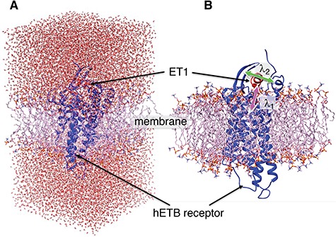
(A) Initial conformation of simulation, and (B) ET1–hETB complex in membrane viewed from a slightly different direction. RCs and are shown, respectively, by magenta and green arrows. Other RCs are shown in Fig. S5.

The mD-VcMD simulation was performed using a program omegagene/myPresto (Kasahara et al., 2016) with the following condition: SHAKE algorithm (Ryckaert et al., 1977) to fix the covalent-bond lengths related to hydrogen atoms, Berendsen thermostat to control temperature (Berendsen et al., 1984), the zero-dipole summation method (Kamiya et al., 2013; Fukuda et al., 2011, 2012) for long-range electrostatic computations, a time-step of 2 fs, and simulation temperature of 300 K. An ensemble resulted from the Berendsen thermostat converges on a canonical distribution for a system of many atoms, whereas it generates a non-physical distribution for a small system (Morishita, 2000). To compute the potential energy, the Amber hybrid force fields (mixture parameter ) (Kamiya et al., 2005) was used for hETB and ET1, the Amber lipid force field for POPC lipid (Dickson et al., 2014), TIP3P model for water molecule (Jorgensen et al., 1983), and force fields for chloride and sodium ions (Joung and Cheatham, 2008). The cholesterol force field was generated as described hereinafter. First, the atomic partial charges were derived by quantum chemical calculations using Gaussian03 (Frisch et al., 2004) at the HF/6-31G^* level, followed by Restrained Electrostatic Potential (RESP) fitting (Bayly et al., 1993). Then, those partial charges were incorporated into a general AMBER force field (GAFF) file (Wang et al., 2004) using Amber tools14 (Salomon-Ferrer et al., 2013).

To raise the sampling efficiency further, a trivial trajectory-parallelization technique was used (Higo et al., 2009; Ikebe et al., 2011), where many independent runs were performed in parallel from different initial conformations. The last snapshot from a run of iteration was used for the initial conformation of the successive run of iteration , although the first iterative runs were initiated from the single conformation (Fig. 2A). The actual number of runs for each iteration was 2176. An ensemble of snapshots picked from the multiple production runs was used to analyze the system properties.

Setting RCs

In the current version of mD-VcMD (Hayami et al., 2018), an RC, , is defined by an inter-centroid distance between two atom groups denoted as and , although RC is definable by various ways in general. We introduced seven RCs by performing preliminary simulations. Consequently, mD-VcMD is given as 7D-VcMD in this article. Supplementary subsection 9, Fig. S5, and Table S2 all provide related details.

We briefly explain RCs: is the ET1–hETB distance. is the gate-width of the binding pocket of hETB. is the distance between hETB and the farthest part of ET1 from hETB in the native complex structure (Fig. S5C), which is introduced for selectively sampling the ET1 orientation, as described in the following section. By the selective sampling, the ET1 orientation was approximately maintained as in the native complex structure. Less-interesting conformations were eliminated from sampling. Furthermore, the computational task was reduced. The other four RCs are introduced to prevent ET1 from unfolding during simulation. Although five RCs were introduced for conformational restraints, these restraints do not affect and of virtual states to be sampled (Higo et al., 2017,b). The RC values for the native complex structure were .

Setting RC zones and selective-sampling technique

We defined the RC zones for and according to Supplementary subsection 10 and Table S3. The zones for were related to those for , as shown in Eq. S18. Those for the other RCs were set by Eq. S19–S22. To maintain the ET1 structure, we set and ().

Furthermore, the selective-sampling technique eliminated some less-interesting conformations from sampling (Supplementary subsections 11 and 12). The ET1 orientation was maintained approximately as in the native complex structure. However, as described later, the ET1 orientational fluctuations were large. The selective sampling worked substantially only when ET1 was outside the binding pocket of hETB.

The original mD-VcMD method was proposed assuming that the zone width is constant (Hayami et al., 2018; Higo et al., 2017a,b). In this study, however, the width is variable (Table S3). Therefore, we modified the sampling method to adjust the variable zone width (Supplementary subsection 13).

Canonical distribution function

The canonical distribution function at 300 K is useful to analyze the sampled snapshots. We present a method to derive the function from mD-VcMD in Supplementary subsection 14.

Conventional canonical MD starting from completely dissociative state

As explained later, mD-VcMD demonstrated an attractive interaction between ET1 and hETB even when ET1 was outside the binding pocket of hETB. To confirm this result, we applied conventional canonical MD. Although the canonical MD has lower sampling efficiency than mD-VcMD, it can sample ET1 motions well outside the binding pocket. In mD-VcMD, furthermore, selective sampling restricted the ET1 orientational motions outside the binding pocket. Consequently, the canonical MD was used to compensate ET1 motions outside the binding pocket obtained from mD-VcMD.

We picked 1088 conformations from snapshots sampled by mD-VcMD, of which ET1–hETB distance was in a range , where ET1 was dissociated completely from hETB. Next, we performed conventional canonical MD runs at 300 K starting from the 1088 conformations for 1.0 ns (1.088  in total) with confining in a narrow range , allowing to move freely. As a result, the ET1 orientation was randomized sufficiently in this narrow range (data not shown). Then, 1088 canonical MD runs of 5 ns (5.44 in total) were performed at 300 K allowing all RCs to move freely. Resultant 1088 sub-trajectories from 4 to 5 ns (1.088 in total) were used for analyses. We infer that this canonical simulation was sufficiently long because the attractive interaction was reproduced, as described later.

Results and Discussion

Virtual state-partitioned probability

The current mD-VcMD comprised 76 iterations, the last iteration of which was the production run. Each iteration consisted of 2168 runs. The production run ( in total) was used for analyses. Actual simulation lengths of the iterations are listed in Table S4.

Only a single state was set for each of (i.e. ; ). Therefore, we omitted in expression of as . Furthermore, because the selective sampling allowed only three states to at each state of (Eq. S27 and Fig. S8B), the conformational variety along was small. Therefore, we expressed in a 2D form by integrating over as

2

Figure 3 is the landscape of from the production runs, which is sufficiently uniform: the error (deviation from an ideally flat defined in Eq. S8) is less than 2 kcal/mol.

Fig. 3.

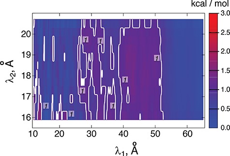
Landscape of converted to potential of mean force, , by and is the gas constant). Its value is presented by the color bar. The lowest is set to 0 kcal/mol. The -th and -th virtual states for and , respectively, are converted to the and axis by and . Numbers labeled near contour lines are PMF values in units of kilocalories per mole.

Free-energy landscape

We also express in a 2D form as

3

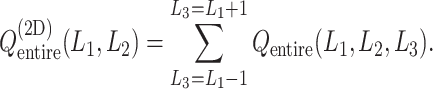
Figure 4A presents the free-energy landscape at 300 K in the 2D plane, where . We picked snapshots from some positions labeled , , … and in the landscape. Fig. 4B portrays those conformations. ET1 was at a native-like position in snapshots and . In snapshots and , ET1 remained in the binding pocket. In snapshots and , ET1 was at the gate of the binding pocket. In snapshots and , ET1 was outside of the binding pocket, whereas ET1 remained contacting some parts of hETB. In snapshots and , ET1 was dissociated from hETB, although ET1 might contact hETB. Finally, in snapshots and , ET1 was dissociated completely from hETB with no contacts.

Fig. 4.

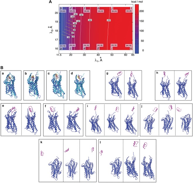
(A) Free-energy landscape expressed by (. Virtual states and are converted to and , as presented in the caption of Fig. 3. The lowest is set to 0 kcal/mol. Numbers labeled near contour liners are their values in units of kilocalories per mole. Conformations taken from positions labeled , , … and are displayed in panel (B). Values are coordinates of the labels in angstrom units. (B) Snapshots taken from labeled positions in panel (A). Each of labels , , , and involves two snapshots, where magenta ET1 and blue hETB construct one snapshot, and yellow ET1 and cyan hETB constitute the other. Two snapshots are displayed for each of , , , and differently to clarify the structural variety. Three snapshots are shown for each label of , , , and .

Here we introduce a notation to express a range of , where the unit of and is angstrom. In Fig. 4A, the free-energy elevation along was apparently steep in , where ET1 was in the binding pocket. Then, the free-energy elevation calmed for . This range involves snapshots and (), where ET1 was at the gate of the binding pocket.

To show the free-energy variation more clearly, we introduced a 1D PMF, , by projecting in the axis. The detailed expression is presented in Supplementary subsection 15. Fig. 5 depicts as a function of . This figure shows again that the free-energy elevation was steep in . We designate this range as a binding pocket range. For , the mean force acting on ET1 from surrounding became weak, and ET1 at was at the gate of binding pocket (snapshots and ). Then, we name as a gate range. In , ET1 was outside of the binding pocket, although still increased slowly with increasing . ET1 contacted hETB in a fraction of snapshots as shown in snapshots , , , and . We name an outside-gate range. For , was almost flat; ET1–hETB contacts were seldom formed. Therefore, the mean force acting on ET1 from surrounding was almost canceled out. In fact, ET1 was completely dissociated from hETB. We designate this range as a completely dissociative range. Fig. S10 summarizes these ranges.

Fig. 5.

(, , ) as function of . The x-axis, which is virtual state originally, is converted to . The conversion method is given in the caption of Fig. 3. Inset is a part of to present differences among , , and .

The inset of Fig. 5 presents an illustration of , which indicates that ET1 can have a path through the open state of the binding gate more readily than through the closed state: in the range of the inset. The probability for the open state is approximately 2000 times greater than that for the closed state. This result indicates that adoption of was effective for enhancing sampling. The in the binding pocket range was also negative, whereas was smaller than that in the gate range.

Fly-casting from mD-VcMD

As shown above, ET1 contacted hETB, even in the outside-gate range. Viewing snapshots in this range, we noticed that ET1 tends to contact three hETB segments: the N-terminal (residues 85–89), a hairpin (residues 241–256), and/or a helix-turn-helix (residues 344–366). We, respectively, denote these segments as , , and (see Fig. 6). They were highly fluctuating in the simulation. Especially, was disordered. was also disordered in crystallography (PDB ID: 5glh). Cys 90 is disulfide-bonding with Cys 358 in hETB. Therefore, the positional fluctuations of Cys 90 were small. Therefore, we did not involve this residue to .

Fig. 6.

Three segments (red ribbon), (green), and (blue). Residue numbers for segments are given in text. Solid lines show the minimum distances . Broken-line rectangle with label S–S denotes a disulfide bond between Cys 90 and Cys 358.

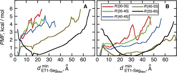
Next, we calculated the heavy-atomic minimum distance between ET1 and each segment for all snapshots. We denote the distances as (), and assigned a contact to a snapshot if . Fig. 7A indicates that most of the contacts were from for . For , and , contacts also appeared. Consequently, the contacts were commonplace in the gate-outside range . Fig. 7A also shows that the contacts appeared even in , which is a part of the completely dissociative range (Fig. S10). However, this contact was minor; non-contacting snapshots were major.

Fig. 7.

Distributions of as function of from (A) mD-VcMD and (B) canonical MD, where is –.

To analyze the contacts further, we calculated a probability distribution of in : . Supplementary subsection 16 explains the method of calculating the distribution. Fig. 8A presents a free-energy basin at except for . A significantly strong attractive force acted between ET1 and in the outside-gate range.

Fig. 8.

as a function of in five ranges of computed from (A) mD-VcMD and (B) canonical MD.

This interaction mechanism should be categorized as a fly-casting mechanism (Arai, 2018; Shoemaker et al., 2000; Sugase et al., 2007), where a disordered protein (or segment) binds weakly and non-specifically to its binding partner. In the present system, once ET1 is captured by the disordered segment , ET1 remains around the binding pocket. Therefore, the local ET1 concentration is raised around the binding pocket even if the concentration is low in the whole solution. Without the disordered tail, hETB cannot capture ET1 from a distant place. The genuine N-terminal of hETB is much longer than the truncated form () in the present simulation. Furthermore, the actual long N-terminal tail might assist the ET1–hETB interactions for longer range (). Later, we discuss the fly-casting mechanism for GPCR-ligand interactions.

Fly-casting from canonical MD

The canonical MD sampled conformations in the completely dissociative and outside-gate ranges. We plot calculated from the 1088 canonical MD runs (1.088 in total) along the axis (Fig. 7B), which showed again that most of the contacts were from for . Comparing Fig. 7B with Fig. 7A, the canonical MD provided a broader distribution than mD-VcMD did at each . This difference is because of the effect of selective sampling used in mD-VcMD, that is, the conventional MD could sample the completely dissociative and outside-gate ranges freely without the restraint on the ET1 orientation. Later, the selective sampling is discussed again.

Figure 8B portrays from the canonical MD, which also presents the free-energy basin at . We conclude that the complex formation was initiated by the fly-casting mechanism.

Variety of intermolecular contacts in the fly-casting mechanism

Here, we analyze the contact in further because this contact was dominant in this range for both simulations (Fig. 7). Four out of five residue sequence of (sequence: ISPPP) are hydrophobic, whereas ET1 (sequence: CSCSSLMDKECVYFCHLDIIW) involves hydrophobic and hydrophilic residues almost equally.

We gathered snapshots involving contacts in . Given a snapshot, if the contact was formed by hydrophobic residues (A, I, L, V, G, P, W, F, and M) of ET1 and , then we judged that this contact was hydrophobic. If it was formed by hydrophilic ones (D, E, K, H, R, T, N, S, Q, Y, and C), then the contact was hydrophilic. The other contacts (i.e. contact between hydrophobic and hydrophilic residues) were assigned as intermediate.

The intermediate-contact fractions were 47.4 and 55.5%. The hydrophobic-contact ones were 42.8 and 40.4%, and the hydrophilic-contact ones were, respectively, 9.8 and 4.1% for mD-VcMD and the canonical MD. Therefore, the largest, second largest, and smallest fractions were, respectively, intermediate, hydrophobic, and hydrophilic commonly whether the selective sampling was used or not. The smallest fraction assigned to the hydrophilic contact results from the small content percentage of hydrophilic residues in .

Figure 9A and 9B, respectively, portray snapshots in from mD-VcMD and canonical MD. From surveying many snapshots in this range, we found that Ile 85 of hETB (the first amino acid residue of ) participated frequently in the contact in both simulations. Contrarily, residues in ET1 had no specificity. Residues labeled in Fig. 9 are those participating in the contact. It is a particularly interesting finding that the contacting residues formed a hydrophobic cluster frequently. This hydrophobic cluster formation occurs readily because Ile 85 of hETB can reach the farthest range from hETB in the currently computed system, and because isoleucine has a long hydrophobic sidechain. Therefore, the hydrophobic cluster tends to be formed first. Met 7 and Lys 9 of ET1 labeled in Fig. 9B are hydrophilic. The stems of these residues are hydrophobic, to which the sidechain of Ile 85 of hETB contacted.

Fig. 9.

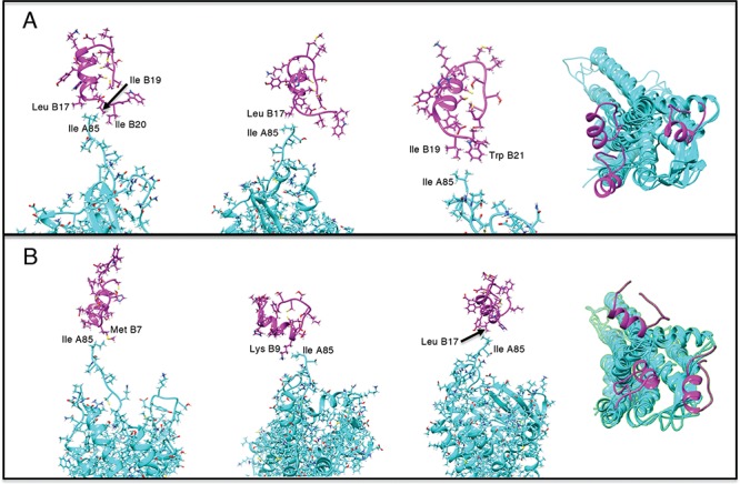
Three snapshots with contact in taken from (A) mD-VcMD and (B) canonical MD. ET1 is in magenta, and hETB in cyan. The right panels are superpositions of the three snapshots. A residue ordinal number in hETB and ET1 is labeled as and , respectively.

Remember that we removed the long N-terminal tail of hETB in the simulation. This tail is disordered in the full-length hETB because the crystallography did not provide the coordinates for the tail. It is also likely that the fly-casting mechanism in the full-length hETB is exerted more effectively than that in the truncated hETB because the disordered long tail can search a longer range around hETB.

Orientations of ET1 relative to hETB

To analyze the effects of selective sampling (Eq. S26) directly, we introduced a scalar product for each snapshot as

4

where and are unit vectors defined, respectively, in ET1 and hETB (Fig. S11). In principle, ranges between and and are completely parallel, then . If completely antiparallel, then .

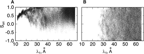
Figure 10A depicts scattering of from mD-VcMD along , where seldom descended below in . This pattern was created by the selective sampling because was not distributed in the full range from to , even in the completely dissociative range . In contrast, from the canonical MD was distributed widely and uniformly in the full range for (Fig. 10B). Because the ET1–hETB interaction becomes weaker with increasing for , it is likely that the canonical MD provided a canonical-like distribution for . Remember that the elimination of zones ( in Eq. S26) in mD-VcMD does not affect the distribution assigned to the sampled zones. Therefore, the canonical MD compensates mD-VcMD in : that is, the sampled region in mD-VcMD is a part of that in the canonical MD for , although the canonical MD could not sample regions for .

Fig. 10.

Distribution of (Eq. 4) as a function of computed from (A) mD-VcMD and (B) canonical MD.

In the gate range , the scattering from mD-VcMD decreased concomitantly with decreasing (Fig. 10A). This decrement occurs because the gate acted on ET1 as an orientational restraint: The selective sampling less affected the ET1 orientation in this range because the lower boundary of the distribution in was apparently larger than that in .

By contrast, the scattering from the canonical MD remained wide in the gate range, although the scattering was considerably sparse (Fig. 10B). Actually, proceeded rarely below in the canonical MD. Therefore, we confirmed again that the binding pocket gate is located at . It is likely that the gate-width is so narrow orientationally that ET1 cannot fit the gate readily, and that once ET1 fits the gate orientationally, the scattering becomes narrower with decreasing up to , as presented in Fig. 10A. This result can be rationalized to define the gate range at .

In mD-VcMD the distribution width of did not vary in , although the position of distribution moved. Therefore, ET1 goes a narrow pathway in the binding pocket to reach the genuine binding form. This range correlates well with the range of the steep free-energy variation in Fig. 5.

Fig. 4A showed no narrow pathway. The ET1–hETB binding/unbinding process can occur via various means in the - plane. As shown in our earlier study (Kamiya et al., 2002), a visual impression of the free-energy landscape depends strongly on the coordinate axes to view the landscape. Although worked effectively for enhancing sampling, another parameter provided a better view to analyze the binding process. The conformational distribution can be constructed in any conformational space once the mD-VcMD sampling is completed.

Multiple contact capture mechanism

With decreasing , other contacts than the one appeared. We analyzed these contacts as follows: Given a snapshot, if all the three minimum distances () were smaller than , then we judged that this snapshot had three contacts. If two, one, or none of the distances were smaller than , then two, one, or no contacts were assigned, respectively, to the snapshot. Then, we calculated a fraction in : , where is the number of snapshots with contacts () in .

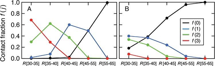
Figure 11A presents the fractions calculated from mD-VcMD. In , and . Then, decreased monotonically with decreasing . Instead, increased rapidly in exhibiting the fly-casting mechanism, and reached the maximum in . Subsequently, decreased quickly in , where reached the maximum. Then, decreased rapidly in because grew quickly in this range. The large in indicates naturally that ET1 contacted all three segments to fit in the binding pocket gate because the gate is constructed by the three segments.

Fig. 11.

(A) Fraction at five ranges of from (A) mD-VcMD and (B) canonical MD.

In the canonical MD (Fig. 11B), was also close to 1.0 in. The other fractions increased gradually with decreasing . However, those fractions did not show the maximum. To fit the gate at , ET1 should contact all the three segments as shown in Fig. 11A. As reported earlier, rarely proceeded below (Fig. 9B). Probably, the orientational disorder of ET1 hindered the three-contact formation. Consequently, ET1 could not penetrate into the binding pocket.

To assess relation between the ET1 orientation and the molecular binding, we picked snapshots randomly from and displayed them in Fig. S12. In , ET1 stayed around the binding pocket gate in both simulations. However, the ET1 orientational variety differed greatly between the two simulations. In mD-VcMD (Fig. S12A), ET1 was able to penetrate among the three segments to move to the gate and binding pocket ranges smoothly by virtue of the convenient ET1 orientation. In the canonical MD (Fig. S12B), by contrast, ET1 was caught at the gate because of the inconvenient molecular orientation of ET1. This point is discussed further later.

Disordered long tail of GPCRs

The cysteine residue at the root of (Cys 90 for hETB), which is conserved in many GPCRs, forms a disulfide bond with a cysteine residue at the N-terminal side of the transmembrane helix 7. The genuine N-terminal tail is long and disordered in many GPCRs (Wallin and von Heijne, 1995). Based on results of the present study, we infer that the long tail captures a ligand before the ligand reaches the binding pocket of GPCR.

The fly-casting mechanism is related to conformational disorder. The conformational disorder can be assigned to either receptor or ligand. The ligand examined in the present study is well structured. The disordered segment of the receptor captures the ligand. A similar fly-casting mechanism was proposed from NMR spectroscopy of another GPCR–ligand complex formation (Kofuku et al., 2009), where a long N-terminal tail of GPCR captures its ligand at an early stage of molecular binding, although there are some differences in the binding process between the two systems.

One might consider that the disordered segment should be folded in the final complex form as shown in the coupled folding and binding mechanism (Higo et al., 2011; Sugase et al., 2007). However, Fig. S12A proposes a different scenario: the figure panels for , , and show that is disordered again. Consequently, works only in the early stage of the ET1–hETB complex formation. This computational result is supported by the result of crystallographic analysis, where is disordered in the complex structure (PDB ID: 5glh), in which the structure of residues 85–87 are not determined.

IDP or intrinsically disordered region (IDR) was discovered from NMR spectroscopy (Wright and Dyson, 1999); the fly-casting mechanism was proposed as an IDP/IDR-related interaction mechanism using a coarse-grained protein model (Shoemaker et al., 2000). Additionally, the conformation-selection and induced-folding (Spolar and Record, 1994) mechanisms are likely to occur in IDP-related interactions. A wide survey (Arai, 2018; Mollica et al., 2016) of NMR spectroscopy and transient kinetic techniques revealed that these interaction mechanisms take place in a mixed manner depending on the system. Results of the present study show that the fly-casting occurred first and that conformation-selection occurred second in the interaction between GPCR and its ligand. Our earlier study (Higo et al., 2011) also showed that conformation-selection and induced-folding take place in a complicated and mixed manner.

Conformational selection at the binding pocket gate of hETB

Decrease of the ET1 orientational variety began at the binding pocket gate () in mD-VcMD (Fig. 10A). Fig. 10B showed that the random orientation of ET1 is inconvenient for ET1 to fit into the gate. Consequently, it is likely that convenient orientations of ET1 are selected from the random orientations to proceed further in the binding process. Generally, this selection mechanism is categorized in conformational selection (or population shift) (Bosshard, 2001; James and Tawfik, 2003; Yamane et al., 2010).

We examined an additional 64 conventional MD runs (13.2 in all) starting from conformations picked from snapshots of mD-VcMD in , which are slightly outside the gate. Those conformations had convenient orientations for molecular binding because they were taken from mD-VcMD. As a result, half of 64 runs moved into the binding pocket, and two runs reached native-like complex forms (data not shown). These results suggest that the ET1 orientation is fundamentally important to fit into the gate. Of course, this simulation does not prove the conformational-selection mechanism firmly. If MD runs are performed for a sufficiently long time starting from random orientations of ET1, then we can confirm the conformational-selection mechanism.

Several points to be improved in the current study

The free-energy difference between the genuine complex structure and the completely dissociated conformations were about 200 kcal/mol (Fig. 5). Reported values of the dissociation constants for complexes of endothelins and their receptors are 1–100 pM in order of magnitude (Hilal-Dandan et al., 1997; Mey et al., 2009; Takasuka et al., 1994). The free-energy differences estimated from these values are about 14–17 kcal/mol. Therefore, the computed free-energy difference is considerably larger than the experimental ones. We infer that the method to update from and (i.e. Eq. S11) might be inaccurate to treat the complicated system. Our earlier work (Higo et al., 2017a) (1D virtual-system coupled Monte-Carlo sampling) presented two equations (Eqs. 4.1 and 4.2 of the article) to update : Eq. 4.1 is fundamentally the same as the present work; actually, Eq. 4.2 is another equation that is suitable for sampling a complicated system or performing non-equilibrium sampling.

Preliminary simulations (Supplementary subsection 9) revealed that ET1 unfolds occasionally in the binding pocket. Consequently, in the present study, we introduced to maintain the tertiary structure of ET1. The free-state ET1 structure from crystallography (Janes et al., 1994) (PDB ID: 1edn) and that from NMR (Takashima et al., 2004) (PDB ID: 1v6r) differ in their details. However, both structures consist of an -helix and an extended strand, between which two disulfide bonds are formed. This overall structural feature of the free ET1 is similar to the bound form used in the present work. We have no information for the transient ET1 structure in the binding pocket. If ET1 unfolds in the binding pocket, then RCs should be modulated to control unfolding and refolding of ET1.

Conclusion

We computed the ET1–hETB free-energy landscape and investigated the ET1–hETB contacts and the ET1 orientations of the sampled snapshots. We classified the ET1–hETB distance into five ranges. In the outside-gate range, the attractive interaction (the fly-casting mechanism) acted between the two molecules, where the disordered N-terminal segment of hETB played an important role. The attractive interaction was confirmed using a conventional simulation method: canonical MD. The present study also suggested the existence of a conformational-selection mechanism, which works at the gate range to select ET1 convenient for transporting ET1 into the binding pocket.

Funding

J.H. was supported by JSPS KAKENHI (Grant No. 16K05517) and by the Development of core technologies for innovative drug development based upon IT from the Japan Agency for Medical Research and Development. J.H. and K.K. were supported by the HPCI System Research Project (Project IDs: hp180050, hp180054, hp190017, and hp190018); mD-VcMD was performed on the TSUBAME3.0 supercomputers at the Tokyo Institute of Technology. K.K. was supported by JSPS KAKENHI (16K18526). H.N. was supported by a Grant-in-Aid for Scientific Research on Innovative Areas (24118008) and a Grant-in-Aid for Challenging Exploratory Research (16K14711) from JSPS. T.H. was supported by OCTOPUS at the Cybermedia Center, Osaka University. This research was conducted in part under the Cooperative Research Program of the Institute for Protein Research, Osaka University, CR-16-05 and CR-19-05. J.H., N.K., and I.F. were supported by Development of Innovative Drug Discovery Technologies for Middle-Sized Molecules from AMED.

This article is for a Special Issue, Computational Design, from Haruki Nakamura, who is an editorial member of PEDS. This is the final revised version after reviewed by two reviewers, Profs. Angela M. Gronenborn and Makoto Kikuchi. Angela is one of the Editorial Board Members of PEDS.

References

- Aldeghi M., Heifetz A., Bodkin M.J., Knapp S. and Biggin P.C. (2016) Chem. Sci., 7, 207–218. [DOI] [PMC free article] [PubMed] [Google Scholar]
- Arai H., Hori S., Aramori I., Ohkubo H. and Nakanishi S. (1990) Nature, 348, 730–732. [DOI] [PubMed] [Google Scholar]
- Arai M. (2018) Biophys. Rev., 10, 163–181. [DOI] [PMC free article] [PubMed] [Google Scholar]
- Athanasiou C., Vasilakaki S., Dellis D., Cournia Z. (2017) J. Comput. Aided Mol. Des., 32, 21–44. [DOI] [PubMed] [Google Scholar]
- Bayly C.I., Cieplak P., Cornell W., Kollman P.A. (1993) J. Phys. Chem., 97, 10269–10280. [Google Scholar]
- Berendsen H.J.C., Postma J.P.M., Gunsteren W.F., DiNola A. and Haak J.R. (1984) J. Chem. Phys., 81, 3684–3690. [Google Scholar]
- Bosshard H.R. (2001) News Physiol. Sci., 16, 171–173. [DOI] [PubMed] [Google Scholar]
- Bowman G.R. and Geissler P.L. (2012) Proc. Natl. Acad. Sci. USA., 109, 11681–11686. [DOI] [PMC free article] [PubMed] [Google Scholar]
- Cimermancic P., Weinkam P., Rettenmaier T.J. et al. (2016) J. Mol. Biol., 428, 709–719. [DOI] [PMC free article] [PubMed] [Google Scholar]
- Clark A.J., Tiwary P., Borrelli K. et al. (2016) J. Chem. Theory Comput., 12, 2990–2998. [DOI] [PubMed] [Google Scholar]
- Dasgupta B., Nakamura H., Higo J. (2016) Chem. Phys. Lett., 662, 327–332. [Google Scholar]
- Dickson C.J., Madej B.D., Skjevik Å.A. et al. (2014) J. Chem. Theory Comput., 10, 865–879. [DOI] [PMC free article] [PubMed] [Google Scholar]
- Frisch M.J., Trucks G.W., Schlegel H.B. et al. (2004) Gaussian 03, Revision E.01. Gaussian, Inc., Wallingford, CT. [Google Scholar]
- Fujitani H., Tanida Y. and Matsuura A. (2009) Phys. Rev. E, 79, 021914. [DOI] [PubMed] [Google Scholar]
- Fukuda I., Kamiya N., Yonezawa Y. and Nakamura H. (2012) J. Chem. Phys., 137, 054314. [DOI] [PubMed] [Google Scholar]
- Fukuda I., Yonezawa Y. and Nakamura H. (2011) J. Chem. Phys., 134, 164107. [DOI] [PubMed] [Google Scholar]
- Fukunishi Y. (2009) Comb. Chem. High Throughput Screen., 12, 397–408. [DOI] [PubMed] [Google Scholar]
- Fukunishi Y. (2010) Expert. Opin. Drug Metab. Toxicol., 6, 835–849. [DOI] [PubMed] [Google Scholar]
- Fukunishi Y., Mikami Y. and Nakamura H. (2003) J. Phys. Chem. B, 107, 13201–13210. [Google Scholar]
- Fukunishi Y. and Nakamura H. (2013) Pharmaceuticals, 6, 604–622. [DOI] [PMC free article] [PubMed] [Google Scholar]
- Gralter F., Schwarzl S.M., Dejaegere A., Fischer S. and Smith J.C. (2005) J. Phys. Chem. B, 109, 10474–10483. [DOI] [PubMed] [Google Scholar]
- Hayami T., Kasahara K., Nakamura H. and Higo J. (2018) J. Comput. Chem., 39, 1291–1299. [DOI] [PubMed] [Google Scholar]
- Hayami T., Higo J., Nakamura H. and Kasahara K. (2019) J. Comput. Chem. , in press (accepted on 17 June 2019). [DOI] [PubMed] [Google Scholar]
- Higo J., Kamiya N., Sugihara T., Yonezawa Y. and Nakamura H. (2009) Chem. Phys. Lett., 473, 326–329. [Google Scholar]
- Higo J., Kasahara K., Dasgupta B. and Nakamura H. (2017a) J. Chem. Phys., 146, 044104. [DOI] [PubMed] [Google Scholar]
- Higo J., Kasahara K. and Nakamura H. (2017b) J. Chem. Phys., 147, 134102. [DOI] [PubMed] [Google Scholar]
- Higo J., Nishimura Y. and Nakamura H. (2011) J. Am. Chem. Soc., 133, 10448–10458. [DOI] [PubMed] [Google Scholar]
- Hilal-Dandan R., Villegas S., Gonzalez A. and Brunton L.L. (1997) J. Pharmacol. Exp. Ther., 281, 267–273. [PubMed] [Google Scholar]
- Iida S., Kawabata T., Kasahara K., Nakamura H., Higo J. (2019) J. Chem. Theory Comput., 15, 2597–2607. [DOI] [PubMed] [Google Scholar]
- Iida S., Nakamura H. and Higo J. (2016) Biochem. J., 473, 1651–1662. [DOI] [PMC free article] [PubMed] [Google Scholar]
- Ikebe J., Sakuraba S. and Kono H. (2014) J. Comput. Chem., 35, 39–50. [DOI] [PubMed] [Google Scholar]
- Ikebe J., Umezawa K., Kamiya N. et al. (2011) J. Comput. Chem., 32, 1286–1297. [DOI] [PubMed] [Google Scholar]
- James L.C. and Tawfik D.S. (2003) Trends Biochem. Sci., 28, 361–368. [DOI] [PubMed] [Google Scholar]
- Janes R.W., Peapus D.H. and Wallace B.A. (1994) Nat. Struct. Biol., 1, 311–319. [DOI] [PubMed] [Google Scholar]
- Jayachandran G., Shirts M.R., Park S. and Pande V.S. (2006) J. Chem. Phys., 125, 084901. [DOI] [PubMed] [Google Scholar]
- Jorgensen W.L., Chandrasekhar J., Madura J.D., Impey R.W. and Klein M.L. (1983) J. Chem. Phys., 79, 926–935. [Google Scholar]
- Joung I.S. and Cheatham T.E. (2008) J. Phys. Chem. B, 112, 9020–9041. [DOI] [PMC free article] [PubMed] [Google Scholar]
- Kamiya N., Fukuda I. and Nakamura H. (2013) Chem. Phys. Lett., 568–569, 26–32. [Google Scholar]
- Kamiya N., Higo J. and Nakamura H. (2002) Protein Sci., 11, 2297–2307. [DOI] [PMC free article] [PubMed] [Google Scholar]
- Kamiya N., Watanabe Y.S., Ono S., Higo J. (2005) Chem. Phys. Lett., 401, 312–317. [Google Scholar]
- Kamiya N., Yonezawa Y., Nakamura H. and Higo J. (2008) Proteins, 70, 41–53. [DOI] [PubMed] [Google Scholar]
- Kasahara K., Ma B., Goto K. et al. (2016) Biophys. Physicobiol., 13, 209–216. [DOI] [PMC free article] [PubMed] [Google Scholar]
- Kofuku Y., Yoshiura C., Ueda T. et al. (2009) J. Biol. Chem., 284, 35240–35250. [DOI] [PMC free article] [PubMed] [Google Scholar]
- Lee M.S. and Olson M.A. (2006) Biophys. J., 90, 864–877. [DOI] [PMC free article] [PubMed] [Google Scholar]
- Levine Z.A., Larini L., LaPointe N.E., Feinstein S.C. and Shea J.-E. (2015) Proc. Natl. Acad. Sci. USA, 112, 2758–2763. [DOI] [PMC free article] [PubMed] [Google Scholar]
- Luzhkov V.B. (2017) Russ. Chem. Rev., 86, 211–230. [Google Scholar]
- Mashimo T., Fukunishi Y., Kamiya N., Takano Y., Fukuda I. and Nakamura H. (2013) J. Chem. Theory Comput., 9, 5599–5609. [DOI] [PubMed] [Google Scholar]
- Mey J.G.R.D., Compeer M.G. and Meens M.J. (2009) Moll. Cel. Pharmacol., 1, 246–257. [Google Scholar]
- Mitsutake A., Sugita Y. and Okamoto Y. (2001) Biopolymers, 60, 96–123. [DOI] [PubMed] [Google Scholar]
- Mobley D.L., Chodera J.D. and Dill K.A. (2007) J. Chem. Theory Comput., 3, 1231–1235. [DOI] [PMC free article] [PubMed] [Google Scholar]
- Mollica L., Bessa L.M., Hanoulle X., Jensen M.R., Blackledge M. and Schneider R. (2016) Front. Mol. Biosci., 3, 52. [DOI] [PMC free article] [PubMed] [Google Scholar]
- Morishita T. (2000) J. Chem. Phys., 113, 2976–2982. [Google Scholar]
- Oleinikovas V., Saladino G., Cossins B.P. and Gervasio F.L. (2016) J. Am. Chem. Soc., 138, 14257–14263. [DOI] [PubMed] [Google Scholar]
- Ostermeir K. and Zacharias M. (2017) PLoS One, 12, e0172072. [DOI] [PMC free article] [PubMed] [Google Scholar]
- Pagadala N.J., Syed K. and Tuszynski J. (2017) Biophys. Rev., 9, 91–102. [DOI] [PMC free article] [PubMed] [Google Scholar]
- Pérez-Benito L., Keränen H., Vlijmen H. and Tresadern G. (2018) Sci. Rep., 8, 4883. [DOI] [PMC free article] [PubMed] [Google Scholar]
- Ryckaert J.-P., Ciccotti G. and Berendsen H.J.C. (1977) J. Comp. Phys., 23, 327–341. [Google Scholar]
- Sakurai T., Yanagisawa M. and Takuwa Y. et al. (1990) Nature, 348, 732–735. [DOI] [PubMed] [Google Scholar]
- Salomon-Ferrer R., Case D.A. and Walker R.C. (2013) WIREs Comput. Mol. Sci., 3, 198–210. [Google Scholar]
- Scior T., Bender A. and Tresadern G. et al. (2012) J. Chem. Inf. Model., 52, 867–881. [DOI] [PubMed] [Google Scholar]
- Shihoya W., Nishizawa T., Okuta A., Tani K., Dohmae N., Fujiyoshi Y., Nureki O. and Doi T. (2016) Nature, 537, 363–368. [DOI] [PubMed] [Google Scholar]
- Shoemaker B.A., Portman J.J. and Wolynes P.G. (2000) Proc. Natl. Acad. Sci. USA, 97, 8868–8873. [DOI] [PMC free article] [PubMed] [Google Scholar]
- Soederhjelm P., Tribello G.A. and Parrinello M. (2012) Proc. Natl. Acad. Sci. USA, 109, 5170–5175. [DOI] [PMC free article] [PubMed] [Google Scholar]
- Spolar R.S. and Record M.T. Jr. (1994) Science, 263, 777–784. [DOI] [PubMed] [Google Scholar]
- Steinbrecher T. and Labahn A. (2010) Curr. Med. Chem., 17, 767–785. [DOI] [PubMed] [Google Scholar]
- Suenaga A., Okimoto N., Hirano Y. and Fukui K. (2012) PLoS One, 7, e42846. [DOI] [PMC free article] [PubMed] [Google Scholar]
- Sugase K., Dyson H.J. and Wright P.E. (2007) Nature, 447, 1021–1025. [DOI] [PubMed] [Google Scholar]
- Sun Z., Yan Y.N., Yang M. and Zhang J.Z.H. (2017) J. Chem. Phys., 146, 124124. [DOI] [PubMed] [Google Scholar]
- Takashima H., Mimura N., Ohkubo T., Yoshida T., Tamaoki H. and Kobayashi Y. (2004) J. Am. Chem. Soc., 126, 4504–4505. [DOI] [PubMed] [Google Scholar]
- Takasuka T., Sakurai T., Goto K., Furuichi Y. and Watanabe T. (1994) J. Biol. Chem., 269, 7509–7513. [PubMed] [Google Scholar]
- Tompa P. and Fuxreiter M. (2008) Trends Biochem. Sci., 33, 2–8. [DOI] [PubMed] [Google Scholar]
- Umezawa K., Ikebe J., Takano M., Nakamura H. and Higo J. (2012) Biomolecules, 2, 104–121. [DOI] [PMC free article] [PubMed] [Google Scholar]
- Lee R., Buljan M., Lang B. et al. (2014) Chem. Rev., 114, 6589–6631. [DOI] [PMC free article] [PubMed] [Google Scholar]
- Villarreal O.D., Yu L., Rodriguez R.A. and Chen L.Y. (2017) Biochem. Biophys. Res. Com., 483, 203–208. [DOI] [PMC free article] [PubMed] [Google Scholar]
- Wallin E. and Heijne G. (1995) Protein. Eng. Des. Sel., 8, 693–698. [DOI] [PubMed] [Google Scholar]
- Wang K., Chodera J.D., Yang Y. and Shirts M.R. (2013) J. Comput. Aided Mol. Des., 27, 989–1007. [DOI] [PMC free article] [PubMed] [Google Scholar]
- Wang J., Deng Y. and Roux B. (2006) Biophys. J., 91, 2798–2814. [DOI] [PMC free article] [PubMed] [Google Scholar]
- Wang W., Wang J. and Kollman P.A. (1999) Proteins, 34, 395–402. [PubMed] [Google Scholar]
- Wang J.M., Wolf R.M., Caldwell J.W., Kollman P.A. and Case D.A. (2004) J. Comput. Chem., 25, 1157–1174. [DOI] [PubMed] [Google Scholar]
- Wright P.E. and Dyson H.J. (1999) J. Mol. Biol., 293, 321–331. [DOI] [PubMed] [Google Scholar]
- Yamane T., Okamura H., Nishimura Y., Kidera A. and Ikeguchi M. (2010) J. Am. Chem. Soc., 132, 12653–12659. [DOI] [PubMed] [Google Scholar]
- Yanagisawa M., Kurihara H., Kimura S. et al. (1988) Nature, 332, 411–415. [DOI] [PubMed] [Google Scholar]
Associated Data
This section collects any data citations, data availability statements, or supplementary materials included in this article.