

Abstract
Background:
Recent work has documented that low-income adults have higher life expectancy in more affluent areas of the US. Less is known about the relationship between area affluence and morbidity in the low-income population.
Objective:
To evaluate the association between the prevalence of chronic conditions among low-income older adults and the economic affluence of a local area
Design:
Cross-sectional association study.
Setting:
Medicare in 2015.
Participants:
6,363,097 Medicare beneficiaries aged 66 to 100 with a history of low income support under Medicare Part D.
Measurements:
Adjusted prevalence of 48 chronic conditions was computed for 736 commuting zones (CZ). Factor analysis was used to assess spatial covariation of condition prevalence and to construct a composite condition prevalence index for each CZ. The association between morbidity and area affluence was measured by comparing the mean of condition prevalence index across deciles of median CZ house values.
Results:
Study participants had a mean age of 77.7 years (SD, 8.2), 67% were female, and 61% white. The crude prevalence of 48 chronic conditions ranged from 72.5 per 100 for hypertension to 0.6 per 100 for post-traumatic stress disorder. The prevalence of 48 examined chronic conditions was highly spatially correlated. Composite condition prevalence was on average substantially lower in more affluent CZs.
Limitations:
Low-income status measured based on Medicare Part D low income subsidy receipt and does not capture individuals not enrolled in Medicare Part D
Conclusion:
Low-income older adults living in more affluent areas of the country are healthier. Further, areas with poor health in the low-income elderly population tend to have a high prevalence of most chronic conditions.
INTRODUCTION
Geographic variation in mortality and morbidity, as well as the association between socio-economic status and health are both widely recognized (1,2,11,3–10). Researchers have documented that there are substantial differences in life expectancy and in causes of death across US geographies, even after accounting for differences in age, sex, and racial composition of different areas (12,13,22–24,14–21). A separate large literature has documented differences in morbidity and mortality between different socio-economic and demographic groups in the US (13,16,32–38,22,25–31). More recently, substantial differences in the income-longevity association were found across geographies (3,39,40). Researchers have documented that adults with income in the first quartile of the income distribution have higher life expectancy in more affluent areas of the United States (39). To the best of our knowledge, there exists limited evidence on the local area variation in morbidity stratified by income using clinical measures of diagnoses and large samples of the US population.
Using 100% of Medicare administrative records, we aimed to assess the association between the prevalence of chronic conditions among low-income older adults and the economic affluence of local areas in the United States. We used the receipt of the low-income subsidy in Medicare Part D pharmaceutical benefit as a measure of low income. We hypothesized that low-income older adults living in more affluent areas of the country are healthier and that areas with poor health in the low-income elderly population tend to have a high prevalence of most chronic conditions.
METHODS
We conducted a cross-sectional association analysis using 100% sample of administrative Medicare records for year 2015. Institutional Review Board of the National Bureau of Economic Research approved this study. 6.4 million older adults with a history of low-income support under the Medicare Part D prescription drug benefit for at least one month in years 2006 to 2015 were included in the study. Medicare Part D program, which enrolls more than 70% of all Medicare beneficiaries in the US, provides cost-sharing and premium subsidies for beneficiaries that have income of less than 150% of the federal poverty line and modest countable assets (41,42). More than 85% of low-income subsidy recipients are enrolled into the program automatically by the Centers for Medicare & Medicaid Services (CMS) (43).
Data Sources
Medicare administrative data for years 2006 to 2015 was obtained from CMS. For the universe of 58.3 million individuals enrolled in Medicare in 2015, Medicare Master Beneficiary Summary File (MBSF) provided information about age, gender, race, SSA county code, Medicare Part D enrollment status, receipt of low income support under Part D, and the time of first diagnosis for 57 chronic conditions tracked by CMS. Individuals’ history of Part D low income subsidy receipt for years 2006 to 2014 was obtained from 2006–2014 MBSF. CMS and The Health Inequality Project (https://healthinequality.org/) provided the mapping of SSA county codes to FIPS codes and in turn to commuting zone codes (CZ), as well as information on the median house prices in each CZ, and whether or not each CZ intersected a Metropolitan Statistical Area (MSA).
Sample
From the universe of Medicare beneficiaries in 2015, individuals were excluded from the study if they lived outside of 50 US states, qualified for Medicare for reasons other than old age, and were younger than 66 or older than 100 years in 2015. We further excluded beneficiaries without Part D enrollment because we were not able to identify their low income status. Finally, we excluded individuals that were never observed to receive low-income subsidies in Part D in 120 months from 2006 to 2015.
Definition of a Local Area and Affluence
A local area was defined as a Commuting Zone, which is a group of counties. This grouping, developed by the Department of Agriculture, reflects commuting patterns between home and work in a local area. We chose this level of geographic aggregation because CZs reflect local economic and social activity ties rather than political boundaries. We use 1990 CZ delineation that splits the US into 741 CZs. Our analytic sample did not include any individuals in five CZs in Alaska, restricting our analysis to 736 CZs. Affluence of each CZ was measured using the median home value in the CZ. House prices incorporate both market and nonmarket (for example, air quality) characteristics of a local area and are an effective summary measure of an area’s socio-economic status (44). We ordered 736 CZs by increasing median house value and divided them into ten equally sized groups, representing deciles of the median home value distribution. Within each group we categorized CZs into urban and rural. A CZ was defined as urban if it intersected an MSA.
Outcomes
An individual was recorded to have one of 48 conditions if we observed the date when this individual first met CMS diagnosis criteria for this condition. The criteria are based on a combination of diagnostic and procedural codes. Indicators for 57 chronic conditions tracked by CMS were available in our data. We excluded 9 conditions with prevalence of less than 0.5 per 100 individuals to ensure enough observations for each condition in each CZ.
Demographic variables
To ensure sufficient sample size within each demographic cell, we discretized age into five disjoint intervals: age 66 to 69; 70 to 74; 75 to 79; 80 to 84; and 85 and older. We created indicator variables for being female and white using sex and race records.
Statistical Analysis
Descriptive data for the whole sample is presented as counts, means and standard deviations. Crude prevalence per 100 individuals was computed for all 48 conditions in the full sample. Crude CZ-level prevalence was adjusted to account for differences in age, race and sex across CZs. The adjustment was done using direct standardization (45). Twenty demographic cells were defined for standardization, using all combinations of indicators for five age intervals, female, and white. This adjustment method allowed for the relationship between prevalence and age to be CZ-specific and to vary flexibly by age and gender. The standard population distribution was computed empirically from the entire analytic sample.
We used factor analysis to assess the spatial covariation of condition prevalences, and to aggregate 48 conditions into a composite CZ-level prevalence index. The share of variance explained by the first factor in factor analysis was used as a measure of covariation across condition prevalences. The composite index was constructed in two steps. First, we computed a regression-based factor score for the first factor in our analysis (46,47). The regression-based factor score is an optimally weighted linear combination of z-scores of condition prevalences in each CZ. Second, to improve interpretability, we rescaled the standardized CZ-level factor score to be an index with mean 100 and standard deviation 10. The resulting local area chronic condition index (LACCI) for low income older adults can be interpreted in percent terms. For example, an LACCI of 150 in a given CZ would suggest that this CZ has a 50% higher composite prevalence of 48 examined conditions relative to an average CZ.
In addition to factor analysis, we used a graphical approach to illustrate the extent of spatial covariation of condition prevalence. We first identified one hundred most populous CZs and ordered them by increasing LACCI. We then created a matrix that - for each CZ in rows - recorded the adjusted prevalence of each condition in columns. We used a color scale from blue (low) to red (high) to color code relatively higher prevalence of a condition across CZs. If the prevalence of all conditions were correlated within a CZ, we would expect that for those CZs with the lowest LACCI, the prevalence of most conditions should be relatively low and hence the share of “blue” cells should be high. Reversely, for those CZs with the highest LACCI, the prevalence of most conditions should be relatively high and hence the share of “red” cells should be high.
In the final step of our analysis we examined the association between LACCI and the deciles of the median home price distribution across CZs. We quantified the magnitude of the association by computing the average LACCI within each decile, separately for urban and rural CZs. We measured the precision of the association using a two-sided t-test that compared the mean LACCI in deciles 1 to 9 to the mean LACCI in decile 10, which had the highest median home values. The p-value of <0.05 was considered to indicate a statistically significant association.
We performed several sensitivity analyses. First, we repeated the analysis using multivariable logistic regression for demographic adjustment. Demographic adjusters were included as main effects for five age groups, and indicators for female and white. We included separate indicators for women in each age group and for white women, which allowed age effects to vary by gender and for the gender effect to vary by race. Standard errors were clustered at the CZ level to account for the hierarchical structure of the data. The logistic regression included indicator variables for each CZ. Adjusted prevalence was predicted for each CZ at the mean of demographic groups in the full sample. Second, we repeated the analysis using direct standardization adjusting for age and gender, but not for race. Third, we repeated the analyses on a subsample of individuals that were observed to live in the same CZ in years 2006 and 2015, thus restricting our analysis to individuals that did not move in ten years before our measurement. Fourth, we examined methods other than factor scores for aggregating 48 conditions into an LACCI, such as a linear combination of condition prevalence that uses national prevalence as weights, or a linear combination of standardized condition prevalence with equal weights.
All analyses were performed in Stata for Unix 15.1/MP.
Role of the Funding Source
The funders had no role in the design or conduct of the study; analysis or interpretation of the data; or preparation of the manuscript.
RESULTS
We identified 40,387,209 individuals in 2015 MBSF who had age between 66 to 100, resided in 50 US States, and were eligible for Medicare because of old age. From these potentially eligible individuals, we excluded 10,568,733 (26%) for whom it was not possible to define Part D low income subsidy status. These individuals either had other sources of prescription drug coverage or had no records of any coverage. We further excluded 13,226 (0.04%) individuals for whom we were not able to match the recorded SSA county codes to FIPS codes. From the remaining 29,805,250, we selected 6,363,097 (21%) into the final analytic sample (Appendix Figure 1). These individuals were observed to have had at least one month of low-income subsidy receipt over 120 months from 2006 to 2015.
Individuals in our analytic sample had a mean age of 77.7 years (SD, 8.2), 67% were female, and 61% were white (Table 1). They had received low income Part D subsidies for 68.1 months on average (SD, 41.3). The crude prevalence of 48 chronic conditions ranged from 72.5 per 100 for hypertension to 0.6 per 100 for post-traumatic stress disorder (Figure 1). Five most prevalent conditions in addition to hypertension were hyperlipidemia, anemia, rheumatoid arthritis and osteoarthritis, ischemic heart disease, diabetes, and depression.
Table 1.
Characteristics of study participants
| n = 6 363 097 | Mean | SD |
|---|---|---|
| Age | 77.7 | 8.2 |
| Female | 0.67 | 0.5 |
| White | 0.61 | 0.5 |
| Months with Part D low-income subsidy* | 68.1 | 41.3 |
Measured in 120 months between 2006 and 2015
Figure 1. Crude prevalence of 48 chronic conditions in the study sample, per 100 individuals*.
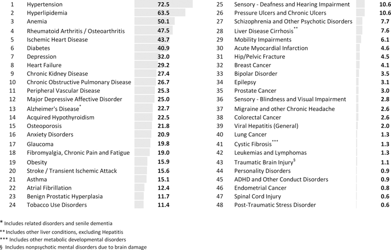
* The study sample includes 6,363,097 low-income older adults observed in year 2015. These individuals were selected from the universe of Medicare beneficiaries in 2015, according to the following criteria: age between 66 to 100, resided in 50 US States, were eligible for Medicare because of old age, had Medicare Part D prescription drug coverage, and were observed to have had at least one month of low-income subsidy receipt over 120 months from 2006 to 2015.
Adjusted prevalence of chronic conditions varied substantially across CZs. Figure 2 illustrates the variation for four common conditions: hypertension, depression, diabetes, and Alzheimer’s Disease and related dementias. The prevalence of hypertension was 75.0 per 100 in an average CZ, but ranged from 34.8 in the CZ around Bethel, AK to 91.9 in the CZ around Lake Providence, LA (SD 10.0, IQR 70.1 to 83.6). The prevalence of diabetes was 38.8 per 100 in an average CZ, but ranged from less than 12 in Alaska to 63.0 in the CZ around Frederick, OK (SD 7.6, IQR 35.2 to 43.6). The prevalence of depression was 34.5 per 100 in an average CZ, but ranged from 7.2 in the CZ around Bethel, AK to 51.1 in the CZ around Cody, WY (SD 5.7, IQR 31.4 to 38.3). The prevalence of Alzheimer’s Disease and related dementias was 22.4 per 100 in an average CZ, but ranged from 4.8 in the CZ around Bethel, AK to 36.3.1 in the CZ around Madison, IN (SD 4.5, IQR 19.6 to 24.4).
Figure 2. Adjusted prevalence, per 100 individuals, of hypertension, diabetes, depression, and Alzheimer’s disease in the study sample across 736 commuting zones*.
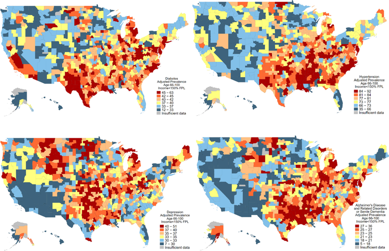
*Age-sex race adjustment was performed using direct standardization. The standardized population was the empirical distribution of 20 demographic categories in the full sample. Demographic categories included all permutations of indicators for female, white, and five age intervals: 66 to 69, 70 to 74, 75 to 79, 80 to 84, and 85 and above. The study sample includes low-income older adults enrolled in Medicare as defined in Table 1 and Figure 1.
The prevalence of 48 examined chronic conditions was highly spatially correlated, with the first factor in factor analysis being able to account for 66% of observed variance, while the second factor contributed only 9% towards cumulative variance (Appendix Table 1). This finding was consistent with the hypothesized spatial pattern - that a CZ with a high prevalence of one condition had high prevalence of most conditions. Factor loadings for the first factor supported this finding, since the first factor was strongly correlated with the prevalence of most conditions (Appendix Table 2).
LACCI for older low-income adults was created using regression-based factor scores. LACCI varied substantially across the United States (Figure 3). The average LACCI was 100 (SD 10) by construction. Among all 736 CZs considered in the analysis, LACCI ranged from 61.7 in the CZ around Bethel, AK to 122.3 in the CZ around Sherman, TX. SD of the index was 10 by construction. The IQR was 94.4 to 106.9 across all 736 CZs. Among one hundred most populous CZs, the average LACCI was 98.1 and ranged from 73.8 in the CZ around Tucson, AZ to 120.0 in the CZ around Detroit, MI (SD 9.2, IQR 91.1 to 102.5).
Figure 3. Local Area Chronic Conditions Index (LACCI) for low-income older adults across 736 commuting zones*.
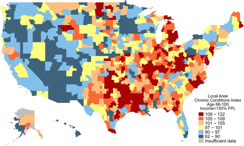
*LACCI is an index that was constructed as a regression-based factor score from factor analysis for prevalence of 48 chronic conditions among low-income older adults in 736 commuting zones. As a result, LACCI measures the aggregate prevalence of chronic conditions among low-income older adults in each commuting zone. A higher LACCI implies a higher average prevalence of chronic condition. The LACCI was standardized to have a mean of 100 and a standard deviation of 10 and can be interpreted in percent terms. For example, an LACCI of 150 in a given commuting zone would suggest that this commuting zone has a 50% higher composite prevalence of 48 examined conditions relative to the average commuting zone.
Graphical analysis in Figure 4 visually illustrates the high degree of spatial covariation across condition prevalences. The figure is restricted to 100 most populous CZs. The CZs index the rows and are ordered top to bottom from the lowest to the highest LACCI. Conditions are ordered in columns left to right from the least to the most nationally prevalent condition. We observe a high share of blue (lower prevalence) cells in the top rows for CZs with the lowest LACCI and a high share of red (higher prevalence) cells in the bottom rows for CZs with the highest LACCI, indicating spatial correlation of prevalences.
Figure 4. Spatial covariation of adjusted prevalence, per 100 individuals, of 48 chronic conditions in 100 most populous commuting zones.*.

* Each cell of the matrix records age-sex-race adjusted prevalence of a chronic condition per 100 individuals. Rows represent commuting zones that are ordered from the lowest (at the top) to the highest (at the bottom) Local Area Chronic Condition Index (LACCI). LACCI measures the aggregate prevalence of chronic conditions among low-income older adults in each commuting zone. A higher LACCI implies a higher average prevalence of chronic conditions. Each column represents a chronic condition. The conditions are ordered by decreasing crude national prevalence from left to right, with the most prevalent condition first. The resulting order of conditions is the same as in Figure 1. Lower prevalence within a column is shaded with blue, while higher prevalence is shared with an increasing intensity of red.
LACCI in the low income older adult population was on average substantially lower in more affluent CZs, as measured by the CZ’s median home value (Figure 5 and Appendix Table 3). This pattern was present in both urban and rural CZs and was nearly perfectly monotone with LACCI falling with higher home value deciles, except for the CZs in the first (lowest) decile of home values that had substantially lower LACCI than CZs in the second decile. Among urban CZs, LACCI in the second decile was 14.5 points higher (1.6 standard deviations difference; 95% CI 5.5 to 23.6; p-value 0.002) than in the top decile (LACCI=95.5). At each decile of home values, rural CZs had on average substantially lower LACCI. The difference was largest in the bottom deciles – 8.2 points (p-value 0.25) and 8.5 points (p-value 0.047) in the first and second lowest deciles, respectively. The difference between LACCI between urban and rural CZs was substantially less pronounced at the top of the home value distribution, with a statistically imprecise difference of 2.4 points in the top decile (p-value 0.37).
Figure 5. Association between Local Area Chronic Conditions Index (LACCI) for low-income older adults and median house values in a commuting zone*.
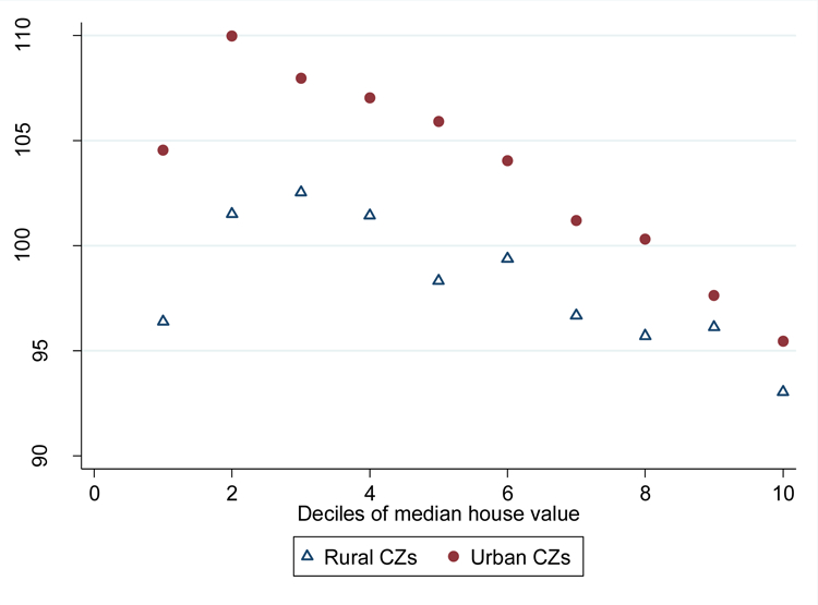
*The plot records the average Local Area Chronic Condition Index (LACCI), on the y-axis, for each decile of commuting-zone level median house values, on the x-axis. LACCI measures the aggregate prevalence of chronic conditions among low-income older adults in each commuting zone. A higher LACCI implies a higher average prevalence of chronic condition. The LACCI has a mean of 100 and a standard deviation of 10 and can be interpreted in percent terms relative to an average commuting zone that has an LACCI of 100. The association between disease burden and the median house value in an area is shown separately for urban and rural commuting zones. A commuting zone was defined to be urban if it intersected a Metropolitan Statistical Area.
The main results remained qualitatively unchanged in our sensitivity analyses that varied the method of demographic adjustment, the method of aggregation of conditions into an index, and the sample. The main differences were observed in models that either did not adjust for race or adjusted for race less flexibly than in the baseline specification. In these models, we observed a more monotone relationship between LACCI and deciles of home values (Appendix Tables 4–6), with no outliers in the first decile. Further, in these models we observed less difference in LACCI between urban and rural CZs. The general pattern of lower LACCI in more affluent CZs and the strong covariation of condition prevalences across CZs were observed in all sensitivity analyses.
DISCUSSION
Our results suggest an important interrelationship between the socio-economic environment of low-income older individuals and their health. We find that low income older adults living in more affluent areas of the country are healthier and that areas with poor health in the low-income elderly population tend to have a high prevalence of most chronic conditions. These results are broadly consistent with the extensive literature on the social determinants of health (1,8,38,48–51). Our study extends this prior research by providing measures of chronic condition prevalence among low-income older adults for a large national sample of the US population, by using clinical rather than self-reported measures of diagnoses, and by reporting the variation in morbidity of low-income older adults across local areas of the country rather than nationally. We draw three key conclusions from our results.
First, the health of low-income older adults in the US varies substantially across local geographies and this variation cannot be attributed to one specific disease or a narrow set of conditions. Local areas tend to be systematically healthy or unhealthy for low- income older adults; in the unhealthy places, the prevalence of most chronic conditions that we examined was high. This evidence suggests that any hypothesized causal pathway that aims to explain the geographic variation in health of the low-income population would need to explain the elevated prevalence of a broad spectrum of diseases in the same area.
Second, we find that low income older adults have better health in rural areas of the country. This difference is especially pronounced in less affluent commuting zones. In the most affluent commuting zones, in turn, the health of individuals living in rural and urban areas was found to be very similar. Multiple mechanisms could explain this finding, including true differences in underlying health that could stem from more manual activity or higher disposable incomes, systematic underdiagnosis of chronic conditions in less affluent rural areas (52–54), or more similarity between urban and rural areas in more affluent parts of the country. More research is needed to understand these patterns.
Finally, consistent with our original hypothesis we find that more affluent local areas of the country have a lower prevalence of chronic conditions in the low-income older adult population. Individuals with the same low level of income are healthier in more affluent areas, even though their income is likely to have less purchasing power in these areas. Taken together, our findings support a number of hypotheses about the role of location for health outcomes as well as the “single-factor” determinant of health hypotheses (8,48,49,55).
Our study has several limitations. First, we use the receipt of low-income subsidies in Medicare Part D as a proxy for low-income status. This is a coarse measure of income that likely undercounts socio-economically disadvantaged individuals and restricts our analysis to individuals with Medicare Part D prescription drug benefit We find that the prevalence of most chronic conditions is substantially higher in our sample of low-income older adults than in the overall Medicare population as reported in CMS statistics (56). This is not surprising, as the prevalence of disease is known to be higher in poorer households, on average. In addition, the CZ-level prevalences that we report adjust for geographic differences in demographics, contributing to the difference between our results and public reports. Our sample likely overstates the average prevalence relative to the full sample of low-income Medicare beneficiaries, as we are more likely to capture the poorest households that are automatically enrolled in Medicare Part D, but could be undercounting near-poor households that may have better health, but not be enrolled in Medicare Part D, or not be receiving low-income subsidies. Further, if in affluent areas healthier individuals are more likely to enroll in Medicare Part D and are also more likely to apply for low-income subsidy relative to less affluent areas, our results could reflect such differential sorting of individuals into the study sample within a CZ in addition to actual differences in condition prevalence across CZs. Second, to measure the prevalence of chronic conditions, we rely on CMS Chronic Condition Warehouse indicators which are constructed using diagnosis and procedures codes from Medicare claims. We thus can only measure formally diagnosed conditions and not the underlying condition prevalence. Further, regional differences in diagnostic intensity could lead us to under or over-estimate the prevalence of conditions in certain geographic areas (52–54). We believe this bias is unlikely to substantively affect our results, since differences in diagnostic practices would likely lead to overestimate the prevalence of conditions in more affluent areas that have more readily available healthcare options, while we find lower prevalence in these areas. Lastly, CMS chronic condition indicators rely on Medicare Fee for Service Claims, implying that individuals that CMS never observed in Fee for Service throughout their Medicare enrollment history may not have their chronic conditions captured in the data. Third, selective migration of healthier individuals to more affluent areas of the country could raise concerns about the interpretation of our results. We conducted a sensitivity analysis that restricted our sample to individuals that lived in the same CZ over a period of ten years prior to our measurement. We find similar results. However, earlier selective migration of healthier individuals to more affluent areas of the country contributes to our findings. It is hence importance to interpret our findings as an association between health and location rather than a causal effect of location on health (57).
In conclusion, we find that the prevalence of chronic conditions in the low-income older adult population varies substantially across local areas in the US, that low-income older adults living in more affluent areas of the country are healthier, and that areas with poor health in the low-income elderly population tend to have a high prevalence of most chronic conditions. These results suggest the likely importance of local place-based public health efforts that target the general health of the population rather than any specific conditions.
Acknowledgments
Grant Support: We gratefully acknowledge support by the National Institutes on Aging grants R21AG052833,P01AG005842–29, and K01AG05984301.
Primary Funding Source: National Institutes on Aging
Disclosures: Dr. Polyakova reports grants from National Institutes of Health (NIH), National Science Foundation (NSF), W.E. Upjohn Institute for Employment Research, and National Institute for Health Care Management during the conduct of the study.
Appendix
Appendix Figure 1:
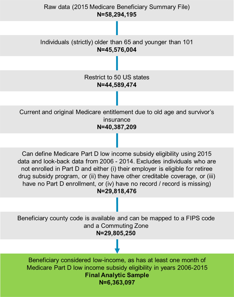
Selection of study participants
Appendix Table 1:
Factor analysis of spatial covariation of adjusted prevalence, per 100 individuals, of 48 chronic conditions in 736 commuting zones
| Factor | Eigenvalue | Share of variance explained |
|---|---|---|
| Factor 1 | 17.9 | 66% |
| Factor 2 | 2.5 | 9% |
| Factor 3 | 1.6 | 6% |
| Factor 4 | 1.4 | 5% |
| Factor 5 | 1.1 | 4% |
| Factor 6 | 0.7 | 2% |
| Factor 7 | 0.5 | 2% |
| Factor 8 | 0.5 | 2% |
| Factor 9 | 0.4 | 2% |
| Factor 10 | 0.4 | 1% |
The results are shown for the first 10 factors only. 27 factors were retained in the model.
Appendix Table 2:
Factor analysis of spatial covariation of adjusted prevalence, per 100 individuals, of 48 chronic conditions in 736 commuting zones
| Condition | Factor loadings | |
|---|---|---|
| Factor 1 | Factor 2 | |
| Anemia | 0.90 | −0.21 |
| Hypertension | 0.90 | −0.17 |
| Hyperlipidemia | 0.88 | −0.23 |
| Rheumatoid Arthritis | 0.87 | −0.15 |
| Ischemic Heart Disease | 0.86 | −0.27 |
| Chronic Kidney Disease | 0.83 | −0.04 |
| Congestve Heart Failure | 0.83 | −0.11 |
| Stroke | 0.81 | −0.08 |
| Anxiety | 0.81 | 0.11 |
| Peripheral Vascular Disease | 0.80 | −0.21 |
| Number of conditions with factor loading >|0.5| | 29 | 0 |
Factor loadings are shown only for ten conditions with the highest correlation with the first factor, but all 48 conditions were included in the model.
Appendix Table 3:
Association between Local Area Chronic Conditions Index (LACCI) for low-income older adults and median house values in a commuting zone, based on prevalence adjusted for age, sex, and race using direct standardization method
| Deciles of median house value distribution | ||||||||||
|---|---|---|---|---|---|---|---|---|---|---|
| 1 | 2 | 3 | 4 | 5 | 6 | 7 | 8 | 9 | 10 | |
| Average LACCI in urban CZs | 104.5 | 110.0 | 108.0 | 107.0 | 105.9 | 104.0 | 101.2 | 100.3 | 97.6 | 95.5 |
| P Value relative to 10th decile | 0.159 | 0.002 | <0.001 | <0.001 | <0.001 | <0.001 | 0.003 | 0.008 | 0.265 | NA |
| Average LACCI in rural CZs | 96.4 | 101.5 | 102.5 | 101.4 | 98.3 | 99.4 | 96.7 | 95.7 | 96.1 | 93.0 |
| P Value, relative to 10th decile | 0.230 | 0.001 | <0.001 | 0.003 | 0.059 | 0.011 | 0.208 | 0.446 | 0.320 | NA |
| P Value, urban versus rural | 0.247 | 0.048 | 0.018 | 0.044 | 0.001 | 0.016 | 0.042 | 0.057 | 0.529 | 0.367 |
| Number CZs, urban | 3 | 6 | 13 | 21 | 35 | 33 | 56 | 54 | 54 | 50 |
| Number CZs, rural | 71 | 68 | 60 | 53 | 38 | 41 | 18 | 19 | 20 | 23 |
Appendix Table 4:
Association between Local Area Chronic Conditions Index (LACCI) for low-income older adults and median house values in a commuting zone, based on prevalence adjusted for age and sex (but not race) using direct standardization method
| Deciles of median house value distribution | ||||||||||
|---|---|---|---|---|---|---|---|---|---|---|
| 1 | 2 | 3 | 4 | 5 | 6 | 7 | 8 | 9 | 10 | |
| Average LACCI in urban CZs | 103.7 | 107.3 | 106.3 | 105.0 | 104.4 | 101.7 | 98.7 | 98.3 | 94.6 | 90.9 |
| P Value relative to 10th decile | 0.077 | 0.002 | <0.001 | <0.001 | <0.001 | <0.001 | <0.001 | <0.001 | 0.094 | NA |
| Average LACCI in rural CZs | 104.6 | 102.9 | 103.3 | 102.8 | 99.4 | 99.2 | 96.2 | 96.9 | 95.7 | 93.7 |
| P Value, relative to 10th decile | <0.001 | <0.001 | <0.001 | <0.001 | 0.041 | 0.036 | 0.350 | 0.261 | 0.443 | NA |
| P Value, urban versus rural | 0.860 | 0.231 | 0.203 | 0.341 | 0.031 | 0.265 | 0.340 | 0.523 | 0.651 | 0.332 |
| Number CZs, urban | 3 | 6 | 13 | 21 | 35 | 33 | 56 | 54 | 54 | 50 |
| Number CZs, rural | 71 | 68 | 60 | 53 | 38 | 41 | 18 | 19 | 20 | 23 |
Appendix Table 5:
Association between Local Area Chronic Conditions Index (LACCI) for low-income older adults and median house values in a commuting zone, based on prevalence adjusted for age, sex and race using logistic regression*
| Deciles of median house value distribution | ||||||||||
|---|---|---|---|---|---|---|---|---|---|---|
| 1 | 2 | 3 | 4 | 5 | 6 | 7 | 8 | 9 | 10 | |
| Average LACCI in urban CZs | 106.3 | 108.5 | 105.5 | 104.4 | 102.6 | 100.4 | 97.9 | 96.9 | 96.1 | 91.8 |
| P Value relative to 10th decile | 0.008 | <0.001 | <0.001 | <0.001 | <0.001 | <0.001 | 0.008 | 0.030 | 0.075 | NA |
| Average LACCI in rural CZs | 105.6 | 103.0 | 104.7 | 100.4 | 99.5 | 98.6 | 95.8 | 98.2 | 94.0 | 93.1 |
| P Value, relative to 10th decile | <0.001 | <0.001 | <0.001 | 0.026 | 0.074 | 0.124 | 0.398 | 0.115 | 0.810 | NA |
| P Value, urban versus rural | 0.818 | 0.040 | 0.692 | 0.113 | 0.234 | 0.496 | 0.396 | 0.568 | 0.539 | 0.735 |
| Number CZs, urban | 6 | 10 | 18 | 25 | 31 | 45 | 47 | 44 | 50 | 48 |
| Number CZs, rural | 56 | 52 | 43 | 37 | 30 | 17 | 15 | 17 | 12 | 13 |
The number of commuting zones is smaller than in direct standardization, since the number of observations in some commuting zones were insufficient to estimate coefficients on the indicator variables for several commuting zones in the maximum likelihood procedure.
Appendix Table 6:
Association between Local Area Chronic Conditions Index (LACCI) for low-income older adults and median house values in a commuting zone, based on prevalence adjusted for age, sex and race using direct standardization method on the sample of individuals that did not move*
| Deciles of median house value distribution | ||||||||||
|---|---|---|---|---|---|---|---|---|---|---|
| 1 | 2 | 3 | 4 | 5 | 6 | 7 | 8 | 9 | 10 | |
| Average LACCI in urban CZs | 103.3 | 110.8 | 107.9 | 106.9 | 106.3 | 104.1 | 101.8 | 100.5 | 99.0 | 97.0 |
| P Value relative to 10th decile | 0.340 | 0.005 | 0.001 | <0.001 | <0.001 | 0.001 | 0.012 | 0.058 | 0.327 | NA |
| Average LACCI in rural CZs | 96.3 | 100.7 | 101.6 | 100.5 | 97.6 | 99.9 | 95.8 | 95.5 | 94.9 | 93.5 |
| P Value, relative to 10th decile | 0.285 | 0.005 | 0.001 | 0.016 | 0.162 | 0.011 | 0.444 | 0.575 | 0.658 | NA |
| P Value, urban versus rural | 0.289 | 0.021 | 0.016 | 0.023 | <0.001 | 0.024 | 0.007 | 0.039 | 0.097 | 0.209 |
| Number CZs, urban | 3 | 6 | 13 | 21 | 35 | 33 | 56 | 54 | 54 | 50 |
| Number CZs, rural | 71 | 68 | 60 | 53 | 38 | 41 | 18 | 19 | 20 | 23 |
Individuals are included in the sample if they are observed to have lived in the same commuting zone over the period of ten years prior to 2015
Footnotes
Publisher's Disclaimer: This is the prepublication, author-produced version of a manuscript accepted for publication in Annals of Internal Medicine. This version does not include post-acceptance editing and formatting. The American College of Physicians, the publisher of Annals of Internal Medicine, is not responsible for the content or presentation of the author-produced accepted version of the manuscript or any version that a third party derives from it. Readers who wish to access the definitive published version of this manuscript and any ancillary material related to this manuscript (e.g., correspondence, corrections, editorials, linked articles) should go to Annals.org or to the print issue in which the article appears. Those who cite this manuscript should cite the published version, as it is the official version of record
Ms. Hua has disclosed no conflict of interest.
Reproducible Research Statement: Original data set: not available due to data use agreement restrictions. Interested researchers can submit an application for a data use agreement at www.resdac.org. Prevalence of 48 conditions, the LACCI measure at the CZ level, and statistical code are available at web.stanford.edu/~mpolyak.
REFERENCES
- 1.Marmot M Social determinants of health inequalities. Lancet 2005; [DOI] [PubMed] [Google Scholar]
- 2.Fuchs VR. Reflections on the socio-economic correlates of health. In: Journal of Health Economics 2004. [DOI] [PubMed] [Google Scholar]
- 3.Case A, Deaton A. Mortality and morbidity in the 21st century. Brookings Pap Econ Act 2017; [DOI] [PMC free article] [PubMed] [Google Scholar]
- 4.Lleras-Muney A Mind the Gap: A Review of The Health Gap: The Challenge of an Unequal World by Sir Michael Marmot . J Econ Lit 2018; [Google Scholar]
- 5.Snyder SE, Evans WN. The effect of income on mortality: Evidence from the social security Notch. Rev Econ Stat 2006; [Google Scholar]
- 6.Preston SH, Kitagawa EM, Hauser PM. Differential Mortality in the United States: A Study in Socioeconomic Epidemiology. J Am Stat Assoc 2006; [Google Scholar]
- 7.Mackenbach JP, Stirbu I, Roskam A-JR, Schaap MM, Menvielle G, Leinsalu M, et al. Socioeconomic inequalities in health in 22 European countries. N Engl J Med 2008; [DOI] [PubMed] [Google Scholar]
- 8.Kawachi I, Berkman L. Social cohesion, social capital, and health. Soc Epidemiol 2000; [Google Scholar]
- 9.Waldron H Mortality differentials by lifetime earnings decile: implications for evaluations of proposed Social Security law changes. Soc Secur Bull 2013; [PubMed] [Google Scholar]
- 10.Duggan JE, Gillingham R, Greenlees JS. Mortality and lifetime income: Evidence from U.S. Social Security Records. IMF Staff Pap 2008; [Google Scholar]
- 11.Braveman PA, Cubbin C, Egerter S, Williams DR, Pamuk E. Socioeconomic disparities in health in the united States: What the patterns tell us. Am J Public Health 2010; [DOI] [PMC free article] [PubMed] [Google Scholar]
- 12.Cullen MR, Cummins C, Fuchs VR. Geographic and racial variation in premature mortality in the U.S.: Analyzing the disparities. PLoS One 2012; [DOI] [PMC free article] [PubMed] [Google Scholar]
- 13.Case A, Deaton A. Rising morbidity and mortality in midlife among white non-Hispanic Americans in the 21st century. Proc Natl Acad Sci 2015; [DOI] [PMC free article] [PubMed] [Google Scholar]
- 14.Dwyer-Lindgren L, Bertozzi-Villa A, Stubbs RW, Morozoff C, Mackenbach JP, van Lenthe FJ, et al. Inequalities in Life Expectancy Among US Counties, 1980 to 2014. JAMA Intern Med 2017; [DOI] [PMC free article] [PubMed] [Google Scholar]
- 15.Dwyer-Lindgren L, Bertozzi-Villa A, Stubbs RW, Morozoff C, Kutz MJ, Huynh C, et al. US county-level trends in mortality rates for major causes of death, 1980–2014. JAMA - J Am Med Assoc 2016; [DOI] [PMC free article] [PubMed] [Google Scholar]
- 16.Mokdad AH, Dwyer-Lindgren L, Fitzmaurice C, Stubbs RW, Bertozzi-Villa A, Morozoff C, et al. Trends and patterns of disparities in cancer mortality among US Counties, 1980–2014. JAMA - J Am Med Assoc 2017; [DOI] [PMC free article] [PubMed] [Google Scholar]
- 17.Roth GA, Dwyer-Lindgren L, Bertozzi-Villa A, Stubbs RW, Morozoff C, Naghavi M, et al. Trends and patterns of geographic variation in cardiovascular mortality among US counties, 1980–2014. JAMA - J Am Med Assoc 2017; [DOI] [PMC free article] [PubMed] [Google Scholar]
- 18.Lochner K, Goodman R, Posner S, Parekh A. Multiple Chronic Conditions Among Medicare Beneficiaries: State-level Variations in Prevalence, Utilization, and Cost, 2011. Medicare Medicaid Res Rev 2013; [DOI] [PMC free article] [PubMed] [Google Scholar]
- 19.Finkelstein A, Gentzkow M, Williams H. Sources of geographic variation in health care: Evidence from patient migration. Q J Econ 2016; [DOI] [PMC free article] [PubMed] [Google Scholar]
- 20.Skinner J. Causes and Consequences of Regional Variations in Health Care. In: Handbook of Health Economics 2011. [Google Scholar]
- 21.Thorpe KE, Howard DH. The Rise In Spending Among Medicare Beneficiaries: The Role Of Chronic Disease Prevalence And Changes In Treatment Intensity. Health Aff 2006; [DOI] [PubMed] [Google Scholar]
- 22.Ezzati M, Friedman AB, Kulkarni SC, Murray CJL. The reversal of fortunes: trends in county mortality and cross-county mortality disparities in the United States. PLoS Med 2008. April;5(4):e66. [DOI] [PMC free article] [PubMed] [Google Scholar]
- 23.Wang H, Schumacher AE, Levitz CE, Mokdad AH, Murray CJL. Left behind: Widening disparities for males and females in US county life expectancy, 1985–2010. Popul Health Metr 2013; [DOI] [PMC free article] [PubMed] [Google Scholar]
- 24.Murray CJL, Mokdad AH, Ballestros K, Echko M, Glenn S, Olsen HE, et al. The state of US health, 1990–2016: Burden of diseases, injuries, and risk factors among US states. JAMA - J Am Med Assoc 2018; [DOI] [PMC free article] [PubMed] [Google Scholar]
- 25.Singh GK, Siahpush M. Widening socioeconomic inequalities in US life expectancy, 1980–2000. Int J Epidemiol 2006; [DOI] [PubMed] [Google Scholar]
- 26.Currie J, Schwandt H. Mortality Inequality: The Good News from a County-Level Approach. J Econ Perspect 2016; [DOI] [PMC free article] [PubMed] [Google Scholar]
- 27.Currie J, Schwandt H. Inequality in mortality decreased among the young while increasing for older adults, 1990–2010. Science (80- ) 2016; [DOI] [PMC free article] [PubMed] [Google Scholar]
- 28.Avendano M, Glymour MM, Banks J, Mackenbach JP. Health disadvantage in US adults aged 50 to 74 years: a comparison of the health of rich and poor Americans with that of Europeans. Am J Public Health 2009. March;99(3):540–8. [DOI] [PMC free article] [PubMed] [Google Scholar]
- 29.Banks J, Marmot M, Oldfield Z, Smith JP. Disease and disadvantage in the United States and in England. JAMA 2006. May;295(17):2037–45. [DOI] [PubMed] [Google Scholar]
- 30.Kershaw KN, Diez Roux AV., Burgard SA, Lisabeth LD, Mujahid MS, Schulz AJ. Metropolitan-level racial residential segregation and black-white disparities in hypertension. Am J Epidemiol 2011; [DOI] [PMC free article] [PubMed] [Google Scholar]
- 31.Davids B-O, Hutchins SS, Jones CP, Hood JR. Disparities in Life Expectancy Across US Counties Linked to County Social Factors, 2009 Community Health Status Indicators (CHSI). J Racial Ethn Heal Disparities 2014; [Google Scholar]
- 32.Meara ER, Richards S, Cutler DM. The gap gets bigger: Changes in mortality and life expectancy, by education, 1981–2000. Health Aff 2008; [DOI] [PMC free article] [PubMed] [Google Scholar]
- 33.Olshansky SJ, Antonucci T, Berkman L, Binstock RH, Boersch-Supan A, Cacioppo JT, et al. Differences in life expectancy due to race and educational differences are widening, and many may not catch up. Health Aff 2012; [DOI] [PubMed] [Google Scholar]
- 34.Dowd JB, Hamoudi A. Is life expectancy really falling for groups of low socio-economic status? Lagged selection bias and artefactual trends in mortality. Int J Epidemiol 2014; [DOI] [PubMed] [Google Scholar]
- 35.Woolf SH, Braveman P. Where health disparities begin: The role of social and economic determinants-and why current policies may make matters worse. Health Aff 2011; [DOI] [PubMed] [Google Scholar]
- 36.Murray CJL, Kulkarni SC, Michaud C, Tomijima N, Bulzacchelli MT, Iandiorio TJ, et al. Eight Americas: investigating mortality disparities across races, counties, and race-counties in the United States. PLoS Med 2006. September;3(9):e260. [DOI] [PMC free article] [PubMed] [Google Scholar]
- 37.Lochner K, Pamuk E, Makuc D, Kennedy BP, Kawachi I. State-level income inequality and individual mortality risk: A prospective, multilevel study. Am J Public Health 2001; [DOI] [PMC free article] [PubMed] [Google Scholar]
- 38.Pickett KE, Wilkinson RG. Income inequality and health: A causal review. Social Science and Medicine 2015. [DOI] [PubMed] [Google Scholar]
- 39.Chetty R, Stepner M, Abraham S, Lin S, Scuderi B, Turner N, et al. The association between income and life expectancy in the United States, 2001–2014. JAMA - J Am Med Assoc 2016; [DOI] [PMC free article] [PubMed] [Google Scholar]
- 40.Lynch JW, Kaplan GA, Pamuk ER, Cohen RD, Heck KE, Balfour JL, et al. Income inequality and mortality in metropolitan areas of the United States. Am J Public Health 1998; [DOI] [PMC free article] [PubMed] [Google Scholar]
- 41.Purcell PJ. Income and Poverty Among Older Americans in 2006. Journal of Pension Planning & Compliance 2008. [Google Scholar]
- 42.Social Security Administration. Amendments to regulations regarding eligibility for a Medicare prescription drug subsidy. Final rule. Fed Regist 2012; [PubMed] [Google Scholar]
- 43.Centers for Medicare and Medicaid Services. CMS Program Statistics, Medicare Part D Enrollment 2015. [Google Scholar]
- 44.Leonard T, Powell-Wiley TM, Ayers C, Murdoch JC, Yin W, Pruitt SL. Property Values as a Measure of Neighborhoods. Epidemiology [Internet] 2016. July;27(4):518–24. Available from: http://insights.ovid.com/crossref?an=00001648-201607000-00011 [DOI] [PMC free article] [PubMed] [Google Scholar]
- 45.Rosenbaum PR. Model-based direct adjustment. J Am Stat Assoc 1987; [Google Scholar]
- 46.THOMSON G THE FACTORIAL ANALYSIS OF HUMAN ABILITY. Br J Educ Psychol 1939; [DOI] [PubMed] [Google Scholar]
- 47.Distefano C, Zhu M, Mîndrilă D. Understanding and Using Factor Scores: Considerations for the Applied Researcher - Practical Assessment, Research & Evaluation. Pract Assessment, Res Eval 2009; [Google Scholar]
- 48.Link BG, Phelan J. Social conditions as fundamental causes of disease. J Health Soc Behav 1995; [PubMed] [Google Scholar]
- 49.Comission on Social Determinants of Health. Closing the gap in a generation. Closing the gap in a generation: Health Equity Through Action on the Social Determinants of Health 2008. [DOI] [PubMed] [Google Scholar]
- 50.Lochner KA, Kawachi I, Brennan RT, Buka SL. Social capital and neighborhood mortality rates in Chicago. Soc Sci Med 2003; [DOI] [PubMed] [Google Scholar]
- 51.Lynch J, Smith GD, Harper S, Hillemeier M, Ross N, Kaplan GA, et al. Is income inequality a determinant of population health? Part 1. A systematic review. Milbank Quarterly 2004. [DOI] [PMC free article] [PubMed] [Google Scholar]
- 52.Finkelstein A, Gentzkow M, Hull P, Williams H. Adjusting Risk Adjustment — Accounting for Variation in Diagnostic Intensity. N Engl J Med 2017; [DOI] [PMC free article] [PubMed] [Google Scholar]
- 53.Welch HG, Sharp SM, Gottlieb DJ, Skinner JS, Wennberg JE. Geographic variation in diagnosis frequency and risk of death among medicare beneficiaries. JAMA - J Am Med Assoc 2011; [DOI] [PMC free article] [PubMed] [Google Scholar]
- 54.Song Y, Skinner J, Bynum J, Sutherland J, Wennberg JE, Fisher ES. Regional variations in diagnostic practices. N Engl J Med [Internet] 2010. July 1 [cited 2015 Jun 9];363(1):45–53. Available from: http://www.pubmedcentral.nih.gov/articlerender.fcgi?artid=2924574&tool=pmcentrez&rendertype=abstract [DOI] [PMC free article] [PubMed] [Google Scholar]
- 55.Wilper AP, Woolhandler S, Lasser KE, McCormick D, Bor DH, Himmelstein DU. A national study of chronic disease prevalence and access to care in uninsured U.S. adults. Ann Intern Med 2008; [DOI] [PubMed] [Google Scholar]
- 56.Centers for Medicare and Medicaid Services. County Level Chronic Conditions Table: Prevalence, Medicare Utilization and Spending [Internet] 2015. [cited 2019 Nov 7]. Available from: https://www.cms.gov/Research-Statistics-Data-and-Systems/Statistics-Trends-and-Reports/Chronic-Conditions/CC_Main.html
- 57.Diez Roux AV Investigating neighborhood and area effects on health. Am J Public Health 2001; [DOI] [PMC free article] [PubMed] [Google Scholar]