Deep Neural Networks for Classification of LC-MS Spectral Peaks

Abstract

Liquid chromatography-mass spectrometry (LC-MS)-based metabolomics has emerged as a valuable tool for biological discovery, capable of assaying thousands of diverse chemical entities in a single biospecimen. Processing of non-targeted LC-MS spectral data requires identification and isolation of true spectral features from the random, false noise peaks that comprise a significant portion of total signals, using inexact peak selection algorithms and time-consuming visual inspection of data. To increase the fidelity and speed of data processing, herein we establish, optimize and evaluate a machine learning pipeline employing deep neural networks as well as a simpler multiple logistic regression model for classification of spectral features from non-targeted LC-MS metabolomics data. Machine learning based approaches were found to remove up to 90% of false peaks from complex non-targeted LC-MS datasets without reducing true positive signals and exhibit excellent reproducibility across multiple datasets. Application of machine learning for non-targeted LC-MS based peak selection provides for robust and scalable peak classification and data filtering, enabling handling and processing of large scale, complex metabolomics datasets.

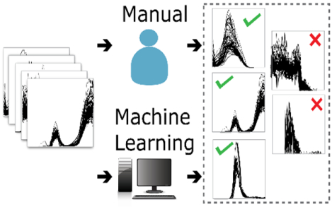
Graphical Abstract

The field of metabolomics has greatly altered the landscape of chemical biology, providing ever expanding insight into the chemical composition of complex biosystems, underpinnings of human disease, and mechanisms of drug responsiveness.^1–3 With the advancement of accelerated high-performance liquid chromatographic (LC) separation approaches coupled to high-resolution mass spectrometry (MS), non-targeted LC-MS based metabolomics approaches are now capable of routine detection of thousands of unique chemical compounds in a single biosample.^4,5 Typical LC-MS experiments further interrogate multiple samples in a single dataset, and increasingly rapid systems allow for hundreds or even thousands of individual samples to be assayed in a single experiment.^5–7 Given the increasing complexity of non-targeted metabolomics data, however, previous reports have suggested that up to 87% of monitored spectral peaks in a given dataset may represent false positive, artifactual features, owing to random detector signals.^8–10 Such false peaks are neither contaminants nor degenerate features¹¹ and cannot easily be distinguished from true positive features using bulk filtering or background control samples and typically have to be removed through manual review.⁸ Removal of false positive peaks is of particular importance in large datasets as they impart a significant statistical penalty and greatly increase the risk of false discovery when comparing metabolite differences among biological groups.^7,12 Given the speed with which vast amounts of non-targeted LC-MS based metabolomics data may now be generated, handling and processing of spectral peaks while accurately discerning true from false spectral signals have collectively become an ever more important bottleneck in the chemical discovery process.

Detection of chromatographic peaks from raw spectral data is a major component of any non-targeted metabolomics pipeline. However, there are a large number of potential methods for performing this task, and common algorithms have multiple adjustable input parameters. As a consequence, vastly different peak lists can be generated from a single raw dataset depending on the algorithm and parameters used. Algorithms for detecting individual spectral peaks range from very simple, such as those that select all chromatogram regions above a certain noise magnitude threshold, to more complex methods that identify peaks using characteristic shape properties, including smoothed second-derivatives, local maxima and minima, or wavelet models.^4,13–16 For instance, the commonly employed centWave algorithm utilizes continuous wavelet transformation for fitting of spectral peaks to a Gaussian shape.¹⁶ Other approaches, including local minimum search, seek local minima or maxima that meet pre-determined shape criteria.¹⁴ While these approaches are capable of consistently identifying abundant chromatographic features exhibiting highly Gaussian peak shapes, their ability to reliably identify features with low intensity, non-gaussian peak shapes, and/or poor baseline resolution, which are typically present in non-targeted LC-MS data, is limited.^10,17 Furthermore, most available algorithms require user tuning of a number of non-intuitive or ‘black box’ input parameters that can have unpredictable consequences for data quality.^8,17 Finally, detector noise can produce signals with shapes similar to true peaks, such that parameter adjustment alone is inadequate to ensure that true peaks are retained and false positives are removed. As such, extensive visual inspection of individual spectral peaks is often required post-processing for further distinguishing of true from false signals, which has become increasingly impractical as datasets become larger with improvements in instrument sensitivity and increasing sample numbers.

With the rapid growth in computing power, deep neural network based machine learning algorithms have emerged as a powerful approach for rapid and accurate classification of images in biomedicine, including for radiographic images,¹⁸ skin lesions,¹⁹ and electrocardiograms,²⁰ among many others.²¹ These deep neural network approaches have the potential to greatly accelerate image processing, and can classify true from false positive images with great accuracy while limiting operator bias. We hypothesized that a deep neural network based machine learning approach would prove effective in “learning” how to properly filter spectral peaks based on thousands of manually curated true and false positive signals, thereby enhancing both data processing speed and reliability. Moreover, given that the specific image features used for classification in deep neural networks are often not clear,^21–23 we also aimed to introduce a simplified secondary machine learning peak classification approach that employs commonly available spectral peak attributes. Collectively these approaches highlight the utility of machine learning for robust processing of non-targeted LC-MS based metabolomics data.

EXPERIMENTAL SECTION

LC-MS metabolomics

Human blood plasma samples from two independent cohorts (Cohort 1 [N = 78] and Cohort 2 [N = 526]) were analyzed using a non-targeted hydrophilic interaction liquid chromatography (HILIC) LC-MS metabolomic approach (See Supporting Information for more details). Raw data was converted to mzXML data format and subsequent extraction of chromatographic features was performed using MZmine 2.¹⁴ This extraction was performed using two different sets of parameters, namely “more restrictive” and “less restrictive” settings (settings provided in Table S1 and Table S2 in Supporting Information), which acted as both a representation of typical MZmine peak lists as well as a baseline for assessing the performance of the neural network and peak parameter models.

Image based deep neural network

To create standardized images for each putative feature, we began by establishing windows (ranges for m/z and retention time) around detected peaks (described in Supporting Information) with bounds set at the lowest start retention time and highest end retention time for a peak group. Given that peak consistency across multiple samples is critical for identification of true signals, stacked peak images were generated for each putative feature using data from samples where the peak was highly prevalent. In order to limit selection bias towards higher abundant peaks, intensity values of each apex were scaled to a maximum intensity of 1. Finally, this data was converted into a 64×64 pixel image raster for each stacked feature in which rows 1 through 63 correspond to peak intensity in 63 different samples. Row 64 was defined as the retention time window boundary for the feature where a pixel value of 1 indicating an active window and a value of 0 indicating an area outside the window. Similar raster images were created for every stacked feature plot, referred to as a peak group, which were then fed into the neural network model for peak classification.

A convolutional neural network model was trained on 1304 manually classified examples of true and false peaks (652 false and 652 true peaks), calibrated on 740 additional examples and tested independently on 726 examples from Cohort 1. The training:calibration:test split was approximately 47%:27%:26%. The neural network model was subsequently tested on data from the independent Cohort 2. In order to test the performance of the neural network model, a randomly selected subset of 3000 peak group examples from the MZmine 2 “more restrictive” dataset were manually classified as well as evaluated using the image based neural network with results compared to assess agreement. The description of training, calibration, and test datasets are described in Table S3 in Supporting Information and examples of peaks that were accepted and rejected by manual review are provided in Figure S1. The architecture of the neural network model was determined empirically by automated tuning of each of the hyperparameters in the model with optimization according to performance in the calibration dataset. The final model was comprised of two hidden convolution layers and two fully connected layers with max-pooling and dropout layers between them. The model architecture is described in detail in Supporting Information.

Peak group parameter model

Six commonly used peak shape attributes were identified that collectively provide a description of overall peak shape, including peak duration, height, area, full-width half max (FWHM), tailing factor, and asymmetry factor. Fifty-nine peak group parameters were defined by mathematical combinations of common statistics of these six shape attributes for aligned peak groups (Table S4) were evaluated based on their ability to statistically distinguish true peaks from false peaks. The 59 peak group parameters were developed based on observations during manual review of peaks and selected based on their potential to separate true peaks from false peaks as evaluated by comparing violin plots of the parameter for true and false peaks and by measure of the average error in k-fold cross validated logistic regression models. The peak group parameter model was trained, calibrated and tested using the same examples as the image based deep neural network. The workflow for generating the peak group parameter model is illustrated in Figure S2 and further described in Supporting Information.

All code used in this paper has been provided to the scientific community at https://github.com/JainLab. The raw data used for generating the images as well as the training, calibration, and test datasets are available at https://doi.org/doi:10.25345/C5FD2F.

RESULTS AND DISCUSSION

In typical non-targeted LC-MS workflows, the complex chemical mixtures present within biosamples are separated, measured, and reported as thousands of discrete chemical measurements with many being of unknown identity (Figure 1A). Mass-to-charge ratio (m/z) values are catalogued from LC-MS data and used to create extracted ion chromatograms for each m/z. Chromatographic peaks are then detected in these chromatograms, typically yielding thousands of spectral features, from which true peaks are selected for further data analysis (Figure 1A). Conventional processing of spectral data using centWave,¹⁶ local minimum search,¹⁴ or other similar algorithms allow for quality filtering of detected peaks; however, adjustment of parameters within these workflows can yield very different outputs depending on the degree of restrictiveness used. For instance, while less restrictive settings will yield a greater number of total features, typically the increase in false positive peaks outscales the increase in true positives, ultimately resulting in false peaks comprising a more significant fraction of total spectral signals (Figure 1B). Conversely, using highly restrictive settings will yield a smaller feature list that’s comprised of mostly high quality features but will have missed many good features due to a higher rate of false negative categorization. As manual inspection of each feature is not feasible at the scale of non-targeted LC-MS experiments, better methods of automated peak filtering need to be developed.

Figure 1.

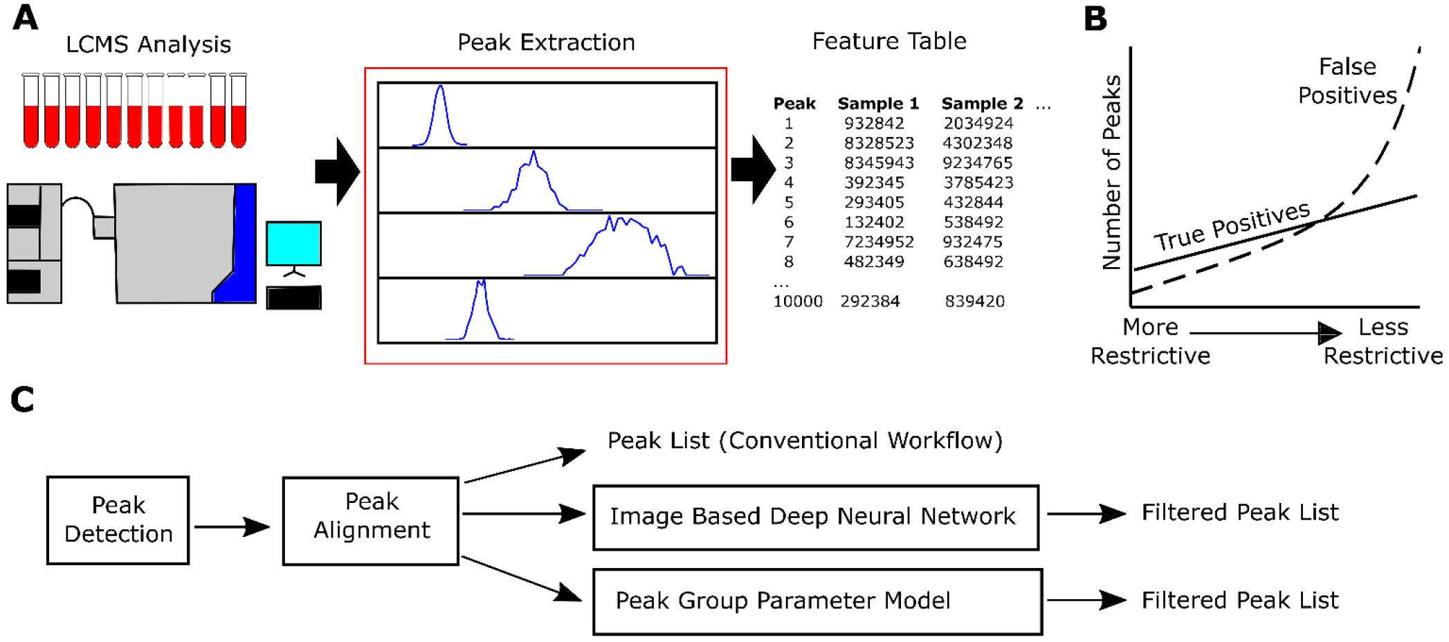
(A) Graphical summary of the LCMS workflow where human plasma was analyzed using non-targeted LC-MS followed by peak extraction using MZmine 2 and creation of candidate peak lists. Peaks of different quality are shown in the red box. (B) An illustration of the observed relationship between the quantities of true positive peaks and false positive peaks as detection parameters are adjusted. (C) A flowchart providing the workflow followed when applying the described models to classify peaks. Peak lists generated in (A) were used to train and evaluate both image based deep neural network as well as peak group parameter models.

Typically, true versus false peak designation is dependent on peak shape quality as well as consistency in shape and retention time across all samples in the study. Most peak selection algorithms, however, only evaluate peak quality on a per sample basis. We therefore sought to develop an image based deep neural network approach as well as a simplified linear regression model that would leverage the advanced decision-making process of a human expert in looking at peak quality across all samples in a study. To this end, human plasma from two independent cohorts (Cohort 1 [N = 78] and Cohort 2 [N = 526]) was analyzed for polar metabolites using a non-targeted HILIC based LC-MS method (See Experimental Section for more information). Non-filtered peak lists were then generated using MZmine 2 where the raw data was extracted using both “More Restrictive” and “Less Restrictive” peak extraction parameters resulting in two peak lists with one being a smaller list of mostly true peaks and the other being a larger list of mostly false peaks, respectively (Table S1 and S2). These two peak lists were then used to train and evaluate both the deep neural network and linear regression quality filtering models (Figure 1C).

Image based deep neural network

In order to train a deep neural network model, peak shape information from the extracted peak lists were converted into images that were readable by both humans and machines for training the model. For human review, stacked peak plots for each extracted feature were produced using peak information from the 63 samples in which the candidate peak was most intense (Figure 2A). Examples of peaks that were accepted and rejected by the human reviewer are provided in Figure S1 in Supporting Information. The structure of the stacked peak plot data can be more clearly represented using a 3D isometric representation (Figure 2B). For input into the deep neural network, the same information can be represented as a raster image in which each pixel value indicates intensity, each row represents a different single sample, and each column represents a different retention time bin (Figure 2C).

Figure 2.

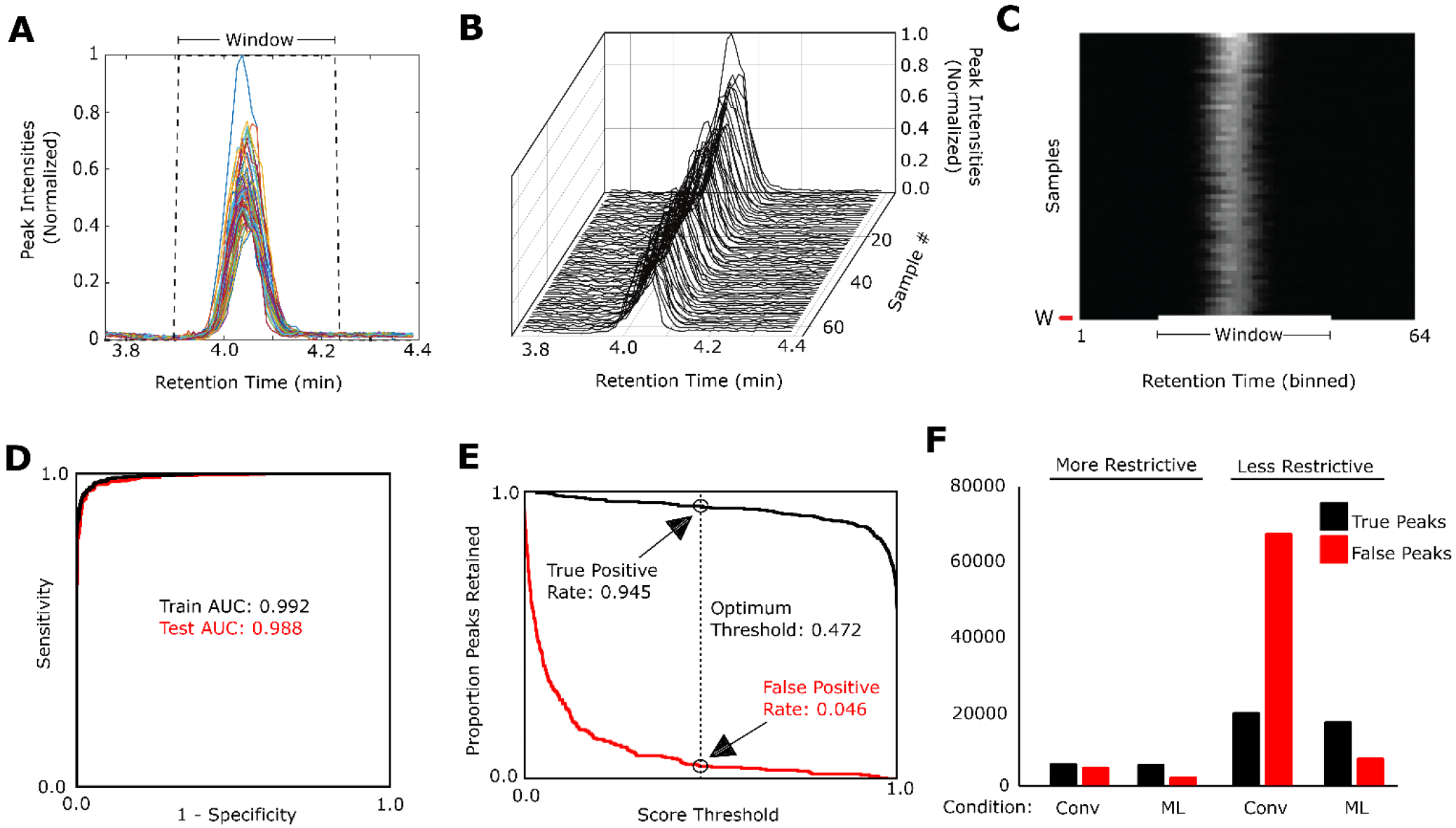
Image based deep neural network model performance (A) A plot of a peak group for a single retention time window. Signal intensity is scaled so the maximum intensity is equal to 1. (B) Scans from multiple samples are considered when determining whether a window contains a true peak. (C) An example peak image generated from signals from multiple samples, where each sample is represented by a single horizontal row. The shade of individual cells indicates the signal intensity. The bottom row indicates the window in which the suspected peak occurs. (D) Receiver-operator curve (ROC) and area under the curve (AUC) for the training and test data sets. (E) A plot of the proportion of true positive (black line) and false positive (red line) peaks retained at each score threshold from zero to one. Values for the optimum score threshold are indicated. (F) A comparison of true positive and false positive peaks retained under 4 conditions. “Conv” refers to peak extraction using a conventional MZmine 2 workflow. This was performed once with typical “More Restrictive” settings and once with “Less Restrictive” settings. “ML” shows the number of peaks retained after the neural network model was applied. Values were determined from manual review of subsets and scaled to reflect the full number of peak groups selected by the MZmine 2 workflows.

The starting peak lists from Cohort 1 were divided into training, calibration and test subsets with 1304 manually reviewed peak examples used for model training (50% true peaks and 50% false peaks), 740 peak examples used for calibration and 726 peak examples used for testing (See Experimental Section for more information). The trained model assigned each peak group a probability score of being a true peak. At each score threshold cutoff value, the true positive rate (sensitivity) and true negative rate (specificity) were determined. Receiver operating characteristic curves (Figure 2D) demonstrated the performance of the machine learning model at each of the thresholds. The curves illustrate an exceptional high specificity and sensitivity with an area under the curve (AUC) of 0.992 and 0.988 in training and test sets, respectively (Figure 2D), indicating that the model is able to mimic the decision making of an expert, integrating visual inputs with prior knowledge and experience, when classifying potential features as false or true peaks in a systematic manner.

For peak selection, an optimum operating point (score threshold) of 0.4725 was selected (see Supporting Information for selection criteria) corresponding to a true positive rate of approximately 0.945, and a false positive rate of approximately 0.04 in the calibration set. Importantly, a different threshold (other than the optimum operating point) may be selected on a case-by-case basis, as dictated by the specific application and dataset in question (Figure 2E). This option allows the user to filter output by peak quality using only a single setting.

The performance of the machine learning approaches was subsequently evaluated on 3000 candidate peaks from Cohort 2 using both “more restrictive” and “less restrictive” settings. Under more restrictive settings conventional peak selection resulted in approximately 50% true positive and 50% false positive peaks, capturing a total of 11,026 features (Figure 2F). Application of the optimized machine learning based neural network to the identical peak windows captured 98% of the true positive peaks and reduced false peak detection by more than 50% (Figure 2F). Under less restrictive settings, a greater number of total peaks were captured, though with a higher proportion of false positive peaks (~75%) (Figure 2F). Under these settings, application of the image based deep neural network peak selection minimally reduced true positive peaks, while drastically improving filtering of false positive peaks by ~90%, substantially improving the overall dataset quality (Figure 2F)

Even with machine learning approaches, a small but notable percentage of peaks still were false positives. Visual inspection of these particular peaks revealed slightly different peak shapes in this independent dataset relative to training datasets, illustrating a common source of retained error with machine learning systems, referred to as covariate shift.^24–26 Common false detected peaks included those with peak splitting outside of the window, shoulder or double peaks, spurious high background peaks, and peaks with low signal to noise (Figure S3). A greater discussion of potential contributors to retained false peaks in image based deep neural network approach is provided in Supporting Information.

While the overall benefit of the image based deep neural network approach for reducing false positive peaks is evident from the data provided, it is likely these algorithms may be even further optimized, particularly through improved understanding of specific causes of peak misclassification, as has been suggested.¹⁵ Additionally, while the machine learning approaches employed specifically within these datasets are somewhat dependent on the characteristics of the LC-MS method, it is likely that data generated using different LC-MS instrumentation and methods will likely only require generation of a new training data set and re-tuning of neural network parameters, rather than re-optimization of multiple settings. Collectively, these data highlight the use of machine learning based neural networks for spectral data handling and peak filtering.

Peak group parameter model

While image based deep neural network-based machine learning models achieve high performance in peak classification, that approach is somewhat opaque and it remains difficult to determine which specific characteristics of the input data are the most important to the deep neural network classifier. We therefore sought to determine whether a simpler classifier based on readily available peak shape attributes would perform comparably to the more complex image based deep neural network approach.

We selected 6 peak shape attributes that are commonly used and collectively provide a good description of peak shape [peak duration, height, area, full-width half max (FWHM), tailing factor, and asymmetry factor], which can be easily exported from MZmine (Figure 3A). Peak group parameters were developed as mathematical combinations of common statistics of the 6 peak shape attributes for groups of aligned peaks. We defined 59 of these peak group parameters that could potentially quantify the observed differences between groups of true and false peaks detected by MZmine 2 (Table S4). Violin plots of each peak group parameter for true and false peaks (Figure 3B) as well as single variable logistic regression models were used to assess the predictive value of individual peak group parameters during development. From among the 59 peak group parameters, the peak group parameter found to be the most predictive of peak quality was medRelFWHM (Figure 3C), calculated as:

$$\mathit{\text{medRelFWHM}}=\mathit{\text{median}}\left(\frac{\mathit{\text{peakFWHM}}}{\mathit{\text{peakduration}}}\right)$$

Figure 3.

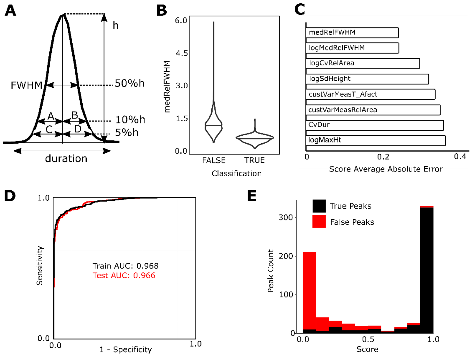
Peak group parameter model (A) Illustration of 6 peak attributes exported from MZmine 2 for prediction. Asymmetry factor = B/A, tailing factor = (C + D)/ (2C). (B) Violin plots comparing the distributions of a single group statistic (medRelFWHM as defined in the main text) of true and false positive peaks (C) The top performing peak group parameters as determined by the average absolute error of the single variable logistic regression model averaged across all folds of a 5-fold cross validation (D) Receiver-operator curve (ROC) and area under the curve (AUC) for the training (black line) and test (red line) data sets. (E) A stacked-bar histogram of peak probability scores predicted by the multiple logistic regression model for false positive (red) and true positive (black) peak groups in the test set.

A multiple logistic regression model was then developed using a forward selection procedure where variables are added one at a time until model improvement stops. This resulted in 15 different peak group parameters being used as variables in the final model (See Supporting Information for the 15 parameters and additional information on model selection). This simple model showed a high level of performance with an AUC on the test set of >0.96 (Figure 3D) and a histogram of the prediction scores (Figure 3E) further illustrates the model’s ability to distinguish between true and false peaks. A Random Forest²⁷ model was also developed from the original 59 peak group parameters and it showed a similar level of performance (Figure S4). Additional information on the Random Forest model is included in Supporting Information.

To compare the performance of this peak group parameter model approach to the image-based deep neural network approach, the 3000 peak groups obtained from Cohort 2 were also classified using the peak group parameter model. At the optimum performance threshold, the image-based deep neural network method retained 88% of true peaks while eliminating 89% of false peaks relative to a conventional peak extraction workflow, whereas the simpler peak group parameter multiple logistic regression model retained the majority of true peaks (80%) and removed a significant portion of false peaks (66%) (Table 1). While the data presented herein as well as in prior reports(28) suggest that deep neural networks may outperform other machine learning approaches, we also find that simpler peak group parameter models may prove useful given their ease of applicability and straightforward implementation using commonly used MZmine 2 workflows and custom R scripts. As such both approaches may be of benefit to LC-MS investigators.

Table 1.

Performance of conventional and machine learning based data extraction approaches

	Conventional Workflow	Image Based Deep Neural Network	Peak Group Parameter Model
True Positives	676	596	539
False Positives	2324	259	792

Application and Limitations

Once properly trained, the machine learning approaches described herein are highly effective at removal of the false peaks that populate non-targeted LC-MS metabolomics datasets. The relationship between the size of the training set and model performance is illustrated in Figure S5. The plot suggests that a model with a high level of performance can be developed with fewer than 1000 peak examples; however the required training set size will be dependent on the specific LC methods. The more discrete the peaks and easier for human classification, the fewer training peaks are required for a high performing model. In contrast, for LC-MS approaches that have many isobaric peaks eluting in a short retention time span or have many peaks present at near baseline noise levels, more training peaks will likely be required for optimum performance. While somewhat variable, manual selection of training peaks and training of a high performing image based neural network or a peak parameter model typically will require on the order of several days time. Importantly, for optimal performance, a peak prediction model must be trained and evaluated for any individual LC-MS method using representative spectral data generated from that specific method. Once trained and evaluated, though, either the image based neural network or a peak parameter model can be used for all future datasets employing the same LC-MS method without a need for re-training or re-optimization, thereby greatly accelerating overall data processing speed. Additionally, while the workflows discussed herein have utilized MZmine 2 for the initial data extraction, the image based neural network only requires that peak groups be represented as m/z-retention time windows. As such, these approaches are amenable to future application as part of other platforms as well as for development of MZmine 2 specific peak filtering modules.

CONCLUSION

Non-targeted LC-MS metabolomics is an invaluable approach for biological discovery. With the improvement in analytical systems and generation of larger and more complex metabolomics datasets, robust approaches for processing of spectral data have become imperative. Due to the large number of variables affecting chromatographic peak shape, traditional peak detection algorithms are incapable of capturing the full variety of legitimate peak shapes created by a single non-targeted LC-MS method, while also avoiding the capture of noise, or unacceptable peaks. In addition, manual peak filtering suffers from inter-and intra-observer bias, low efficiency and performance inconsistency. Herein we developed, optimized, and applied an image based deep neural network model for peak classification, and found this approach to greatly improve upon current peak selection workflows, reducing false peaks by approximately 90%. Moreover, we found that simpler machine learning approaches, such as those using multiple logistic regression models developed from well described peak shape attributes, can also significantly improve upon existing peak detection methods. This work provides an important proof of concept and is the first to our knowledge to demonstrate the potential value of machine learning approaches for LC-MS based spectral peak filtering.

REFERENCES

- (1).Johnson CH; Ivanisevic J; Siuzdak G Metabolomics: beyond biomarkers and towards mechanisms. Nature Review Molecular and Cell Biology 2016. 10.1038/nrm.2016.25. [DOI] [PMC free article] [PubMed] [Google Scholar]
- (2).Patti GJ; Yanes O; Siuzdak G Metabolomics: the apogee of the omic trilolgy. Nature Review Molecular and Cell Biology 2013, 13 (4), 263–269. 10.1038/nrm3314.Metabolomics. [DOI] [PMC free article] [PubMed] [Google Scholar]
- (3).Kaddurah-Daouk R; Weinshilboum R Metabolomic signatures for drug response phenotypes: Pharmacometabolomics enables precision medicine. Clinical Pharmacology and Therapeutics 2015, 98 (1), 71–75. 10.1002/cpt.134. [DOI] [PMC free article] [PubMed] [Google Scholar]
- (4).Smith CA; Want EJ; O’Maille G; Abagyan R; Siuzdak G XCMS: Processing Mass Spectrometry Data for Metabolite Profiling Using Nonlinear Peak Alignment, Matching, and Identification. Analytical Chemistry 2006, 78 (3), 779–787. 10.1021/ac051437y. [DOI] [PubMed] [Google Scholar]
- (5).Watrous JD; Henglin M; Claggett B; Lehmann KA; Larson MG; Cheng S; Jain M Visualization, Quantification, and Alignment of Spectral Drift in Population Scale Untargeted Metabolomics Data. Analytical Chemistry 2017, 89 (3), 1399–1404. 10.1021/acs.analchem.6b04337. [DOI] [PMC free article] [PubMed] [Google Scholar]
- (6).Watrous JD; Niiranen TJ; Lagerborg KA; Henglin M; Xu Y-J; Rong J; Sharma S; Vasan RS; Larson MG; Armando A; et al. Directed Non-targeted Mass Spectrometry and Chemical Networking for Discovery of Eicosanoids and Related Oxylipins. Cell Chemical Biology 2019, 26 (3), 433–442.e4. 10.1016/j.chembiol.2018.11.015. [DOI] [PMC free article] [PubMed] [Google Scholar]
- (7).Ganna A; Fall T; Salihovic S; Lee W; Broeckling CD; Kumar J; Hägg S; Stenemo M; Magnusson PK; Prenni JE; et al. Large-scale non-targeted metabolomic profiling in three human population-based studies. Metabolomics 2016, 12 (1), 1–13. 10.1007/s11306-015-0893-5. [DOI] [Google Scholar]
- (8).Coble JB; Fraga CG Comparative evaluation of preprocessing freeware on chromatography/mass spectrometry data for signature discovery. Journal of Chromatography A 2014, 1358, 155–164. 10.1016/j.chroma.2014.06.100. [DOI] [PubMed] [Google Scholar]
- (9).Mahieu NG; Huang X; Chen YJ; Patti GJ Credentialing features: A platform to benchmark and optimize untargeted metabolomic methods. Analytical Chemistry 2014, 86 (19), 9583–9589. 10.1021/ac503092d. [DOI] [PMC free article] [PubMed] [Google Scholar]
- (10).Myers OD; Sumner SJ; Li S; Barnes S; Du X Detailed Investigation and Comparison of the XCMS and MZmine 2 Chromatogram Construction and Chromatographic Peak Detection Methods for Preprocessing Mass Spectrometry Metabolomics Data. Analytical Chemistry 2017, 89 (17), 8689–8695. 10.1021/acs.analchem.7b01069. [DOI] [PubMed] [Google Scholar]
- (11).Mahieu NG; Patti GJ Systems-Level Annotation of a Metabolomics Data Set Reduces 25 000 Features to Fewer than 1000 Unique Metabolites. Analytical Chemistry 2017, 89 (19), 10397–10406. 10.1021/acs.analchem.7b02380. [DOI] [PMC free article] [PubMed] [Google Scholar]
- (12).Bictash M; Ebbels TM; Chan Q; Loo RL; Yap IK; Brown IJ; De Iorio M; Daviglus ML; Holmes E; Stamler J; et al. Opening up the “black box”: Metabolic phenotyping and metabolome-wide association studies in epidemiology. Journal of Clinical Epidemiology 2010, 63 (9), 970–979. 10.1016/j.jclinepi.2009.10.001. [DOI] [PMC free article] [PubMed] [Google Scholar]
- (13).Savitzky A; Golay MJE Smoothing and Differentiation of Data by Simplified LEast Squares Procedures. Analytical Chemistry 1964, 36 (8), 1627–1639. [Google Scholar]
- (14).Pluskal T; Castillo S; Villar-Briones A; Orešič M MZmine 2: Modular framework for processing, visualizing, and analyzing mass spectrometry-based molecular profile data. BMC Bioinformatics 2010, 11 (1), 395 10.1186/1471-2105-11-395. [DOI] [PMC free article] [PubMed] [Google Scholar]
- (15).Myers OD; Sumner SJ; Li S; Barnes S; Du X One Step Forward for Reducing False Positive and False Negative Compound Identifications from Mass Spectrometry Metabolomics Data: New Algorithms for Constructing Extracted Ion Chromatograms and Detecting Chromatographic Peaks. Analytical Chemistry 2017, 89 (17), 8696–8703. 10.1021/acs.analchem.7b00947. [DOI] [PubMed] [Google Scholar]
- (16).Tautenhahn R; Böttcher C; Neumann S Highly sensitive feature detection for high resolution LC/MS. BMC Bioinformatics 2008, 9 (1), 504 10.1186/1471-2105-9-504. [DOI] [PMC free article] [PubMed] [Google Scholar]
- (17).Rafiei A; Sleno L Comparison of peak-picking workflows for untargeted liquid chromatography/high-resolution mass spectrometry metabolomics data analysis. Rapid Communications in Mass Spectrometry 2014, 29 (1), 119–127. 10.1002/rcm.7094. [DOI] [PubMed] [Google Scholar]
- (18).Lakhani P; Sundaram B Deep Learning at Chest Radiography: Automated Classification of Pulmonary Tuberculosis by Using Convolutional Neural Networks. Radiology 2017, 284 (2), 574–582. 10.1148/radiol.2017162326. [DOI] [PubMed] [Google Scholar]
- (19).Esteva A; Thrun S; Swetter SM; Novoa RA; Blau HM; Kuprel B; Ko J Dermatologist-level classification of skin cancer with deep neural networks. Nature 2017, 542 (7639), 115–118. 10.1038/nature21056. [DOI] [PMC free article] [PubMed] [Google Scholar]
- (20).Hannun AY; Rajpurkar P; Haghpanahi M; Tison GH; Bourn C; Turakhia MP; Ng AY Cardiologist-level arrhythmia detection and classification in ambulatory electrocardiograms using a deep neural network. Nature Medicine 2019, 25 (1), 65–69. 10.1038/s41591-018-0268-3. [DOI] [PMC free article] [PubMed] [Google Scholar]
- (21).Topol EJ High-performance medicine: the convergence of human and artificial intelligence. Nature Medicine 2019, 25 (1), 44–56. 10.1038/s41591-018-0300-7. [DOI] [PubMed] [Google Scholar]
- (22).Castelvecchi D Can we open the black box of AI? Nature 2016, No. 538, 20–23. [DOI] [PubMed] [Google Scholar]
- (23).Mahendran A; Vedaldi A Understanding Deep Image Representations by Inverting Them. 2015 IEEE Conference on Computer Vision and Pattern Recognition (CVPR) 2015. [Google Scholar]
- (24).Shimodaira H Improving predictive inference under covariate shift by weighting the log-likelihood function. Journal of Statistical Planning and Inference 2000, 90, 227–244. [Google Scholar]
- (25).Sugiyama M Sample Selection Bias – Covariate Shift: Problems, Solutions, and Applications. 2007, 8, 985–1005. [Google Scholar]
- (26).Bickel S; Scheffer T Discriminative Learning Under Covariate Shift. Journal of Machine Learning Research 2009, 10, 2137–2155. [Google Scholar]
- (27).Breiman L Random Forests. Machine Learning 2001, No. 45, 5–32. 10.1023/A:1010933404324. [DOI] [Google Scholar]
- (28).Risum AB; Bro R Using Deep Learning to Evaluate Peaks in Chromatographic Data. Talanta 2019, 204 (May), 255–260, DOI: 10.1016/j.talanta.2019.05.053 [DOI] [PubMed] [Google Scholar]
Associated Data
This section collects any data citations, data availability statements, or supplementary materials included in this article.