Inferring effective forces for Langevin dynamics using Gaussian processes

Abstract

Effective forces derived from experimental or in silico molecular dynamics time traces are critical in developing reduced and computationally efficient descriptions of otherwise complex dynamical problems. This helps motivate why it is important to develop methods to efficiently learn effective forces from time series data. A number of methods already exist to do this when data are plentiful but otherwise fail for sparse datasets or datasets where some regions of phase space are undersampled. In addition, any method developed to learn effective forces from time series data should be minimally a priori committal as to the shape of the effective force profile, exploit every data point without reducing data quality through any form of binning or pre-processing, and provide full credible intervals (error bars) about the prediction for the entirety of the effective force curve. Here, we propose a generalization of the Gaussian process, a key tool in Bayesian nonparametric inference and machine learning, which meets all of the above criteria in learning effective forces for the first time.

I. INTRODUCTION

Compressing complex and noisy observations into simpler effective models is the goal of much of biological and condensed matter physics.^1–4 Although there are many models of reduced dynamics, in this proof-of-principle work, we focus on the Langevin equation^5–8 to describe the time evolution of a spatial degree of freedom such as a particle’s position in physical space or the distance between two marked locations (such as labeled protein sites). The Langevin equation is governed by deterministic as well as random (thermal) forces dampened by frictional forces.⁹

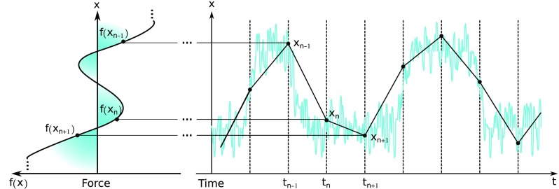
Concretely, the ability to infer effective forces (Fig. 1) from sequences of data, here on in “time traces,” is especially useful in (1) quantitative single molecule analysis^10–15 that has revealed many interesting phenomena well modeled within a Langevin framework, for example, confinement,^16–18 and (2) molecular dynamics (MD) simulations where effort has already been invested in approximating exact force fields with coarse-grained potentials.^19–25 The key behind these coarse-grained force fields is to capture the complicated effects of the extra- or intra-molecular environment on the dynamics of a degree of freedom of interest without invoking atomistic details.

FIG. 1.

Illustration of the goal of the analysis presented. A scalar degree of freedom, x, such as a particle’s position or an intra-molecular distance, is measured at discrete time levels, t_n. The measurements obtained, x_n, in turn, are used to find an effective force f(x). Despite the discrete measurements, the effective force found is a continuous function over x and also extends over positions that may not necessarily coincide with the measured ones x_n.

Naïvely, to obtain an effective force from such a time trace, we would create a histogram for the positions in the time trace ignoring time, take the logarithm of the histogram to find the potential invoking Boltzmann statistics, and then calculate the gradient of the potential.⁵ In practice, this naïve method requires arbitrary histogram bin size selection and large amounts of data to converge and incorrectly estimates the effective force in oversampled and undersampled regions.²⁶ Additionally, such a method does not provide any means to assess the quality of the derived force (e.g., error bars).

Ideally, a method to learn effective forces from time series data would be (1) minimally a priori committal to the effective force’s profile, (2) provide full credible intervals (error bars) about the prediction, and (3) exploit every data point without down-sampling such as binning or pre-processing. Bayesian methods that satisfy the first two criteria above^26,27 exist; however, these methods do not cover the last criteria.

Existing methods are not free of pre-processing such as spatial segmentation and losing information through averaging the force in each spatial segment.^26,27 Neither of these, or similar pre-processing steps, are major limitations when vast amounts of data are available. Yet, data are quite often limited in both MD trajectories and experiments on account of limited computational resources (in silico) or otherwise damaging (in vitro) or invasive (in vivo) experimental protocols.²⁸ These limitations highlight once more the importance of exploiting the information encoded in each data point as efficiently as possible.

To develop a method satisfying all three criteria, we use tools within Bayesian nonparametrics, in particular Gaussian processes (GPs).²⁹ Nonparametrics are required because force is a continuous function, and so learning it cannot be achieved through conventional Bayesian statistics,^30,31 which are restricted to learning collections of scalar parameters. We use GPs as priors to learn the effective forces from a time trace. We show that when data are limited, our method outperforms the existing methods requiring discretization because our method allows inference over the entire space including undersampled (and altogether unsampled) regions. In addition, as we will demonstrate, our method converges to a more accurate force with fewer data points as compared to the existing methods and naturally provides error bars.

II. METHODS

Here, we set up both the dynamical (Langevin) model and discuss the inference strategy to learn the effective force from data. As with all methods within the Bayesian paradigm,^3,28,30–32 we provide not only a point estimate for the maximum a posteriori (MAP) effective force estimate but also achieve full posterior inference with credible intervals.

A. Dynamics model

For concreteness, we start with one dimensional overdamped Langevin dynamics given by⁹

$$\zeta \dot{x}=f\left(x\right)+r\left(t\right),$$ (1)

where x(t) is the position coordinate at time t, $\dot{x}$ is the velocity, f(x) is the effective force at position x, and ζ is the friction coefficient. The thermal force, r(t), is stochastic and has moments

$$⟨r\left(t\right)⟩=0,$$ (2)

$$⟨r\left(t\right)r\left(t^{\prime }\right)⟩=2\zeta kT\delta \left(t-t^{\prime }\right),$$ (3)

where ⟨·⟩ denotes the ensemble averages over realizations, T is the temperature, and k is Boltzmann’s constant.

The positional data from the time trace are x_1:N. These positions, x_n = x(t_n), are indexed with n being the time level label, where n = 1, …, N. In this study, we assume that the time levels t_n are known. Furthermore, we assume that the step size, τ = t_n+1 − t_n, is constant throughout the entire trace x_1:N, although we can easily relax this requirement.

Our assumed model in Eq. (1) is overdamped. Additionally, our model is noiseless, meaning that there is no observation error, as would be relevant to MD or experiments with a high signal to noise ratio. The noiseless assumption is valid when observation error, which we do not incorporate in the present formulation, is much smaller than the kicks induced by the thermal force r(t).

B. Inference model

Given the dynamical model and the time trace, x_1:N, our goal is to learn the force at each point in space, f(·) (normally, we would write f(x), but this might be misleading as it is unclear if it means the function f or the value of the function evaluated at x), and the friction coefficient, ζ. As illustrated in Fig. 1, we only know x₁, …, x_N and our goal is to infer f(·). To achieve this, we use the Bayesian paradigm and try to compute $\mathcal{P}\left(f\left(\cdot \right),\zeta |{\mathit{x}}_{1:N}\right)$. Using Bayes’ theorem, which gives the probability of the model given the data, we obtain

$$\mathcal{P}\left(f\left(\cdot \right),\zeta |{\mathit{x}}_{\mathbf{2}:\mathbf{N}}\right)=\frac{\mathcal{P}\left({\mathit{x}}_{\mathbf{1}:\mathbf{N}}|f\left(\cdot \right),\zeta ,x_1\right)\mathcal{P}\left(f\left(\cdot \right),\zeta \right)}{\mathcal{P}\left({\mathit{x}}_{\mathbf{1}:\mathbf{N}}\right)},$$ (4)

where $\mathcal{P}\left(\cdot \right)$ represents the “probability of the argument” and ·|· stands for “the left argument given right argument.” For the prior, $\mathcal{P}\left(f\left(\cdot \right),\zeta \right)$, we propose a zero-mean Gaussian process (GP) prior on f(·) and an independent Gamma prior on ζ. That is, in the language of statistics, we write

$$f\left(\cdot \right)\sim \mathbf{\text{GP}}\left(0,K\left(\cdot ,\cdot \right)\right),$$ (5)

$$\zeta \sim \mathbf{\text{Gamma}}\left(\alpha ,\beta \right),$$ (6)

where · ∼ · means the “left argument variable sampled from right argument distribution.”

As the data likelihood (discussed below) assume a Gaussian form on f(·) for the thermal kicks, the posterior on f(·)|ζ, x_1:N is also a GP by conjugacy. That is, from our GP posterior, we may sample continuous curves f(·). To carry out our computations, we evaluate this curve on test points, ${\mathit{x}}_{1:M}^{*}$, that may be chosen arbitrarily. Specifically, we evaluate either ${\mathit{f}}_{\mathbf{1}:\mathbf{M}}^{*}$ or ${\mathit{f}}_{\mathbf{1}:\mathbf{M}}^{*}|\zeta ,{\mathit{x}}_{1:N}$, where $f_m^{*}=f\left(x_m^{*}\right)$ (see the supplementary material). Because the GP allows us to choose the test points ${\mathit{x}}_{1:M}^{*}$ arbitrarily, including their number M and the specific position $x_m^{*}$ or each one, our ${\mathit{f}}_{1:M}^{*}$ and ${\mathit{f}}_{1:M}^{*}|\zeta ,{\mathit{x}}_{1:M}^{*}$ are equivalent to the entire functions f(·) and f(·)|ζ, x_1:N, respectively. In other words, using the test points ${\mathit{x}}_{1:M}^{*}$, we do not introduce any discretization or any approximation error whatsoever.

1. Constructing the likelihood

The shape of the likelihood in Eq. (4) is itself dictated by the physics of the thermal kicks, i.e., in this case, uncorrelated Gaussian kicks [Eq. (1)]. To find the likelihood for a time trace of positions, x_1:N, we consider the following discretized overdamped Langevin equation under the forward Euler scheme:^6,33

$$\frac{\zeta }{\tau }\left(x_{n+1}-x_n\right)=f\left(x_n\right)+r_n,$$ (7)

where $r_n\sim \mathbf{\text{Normal}}\left(\mathrm{0,2}\zeta kT/\tau \right)$. The forward Euler scheme [Eq. (7)] is a first order, discretized approximation of the dynamics meaning that it is valid when the data acquisition rate is sufficiently high (i.e., when τ is sufficiently small). Since r_n is a normal random variable, the change in position x_n+1 − x_n|x_n is also a Normal random variable. In fact, rearranging Eq. (7), we obtain

$$x_{n+1}|f\left(\cdot \right),\zeta ,x_n\sim \mathbf{\text{Normal}}\left(\frac{\tau }{\zeta }f\left(x_n\right)+x_n,\frac{2\tau kT}{\zeta }\right).$$ (8)

Assuming a known initial position, x₁, the likelihood of the rest of the time trace is then the product of each of these normals

$$\mathcal{P}\left({\mathit{x}}_{2:N}|f\left(\cdot \right),\zeta ,x_1\right)=\prod _{n=2}^N\mathbf{\text{Normal}}\left(x_n;\frac{\tau }{\zeta }f\left(x_{n-1}\right)+x_{n-1},\frac{2\tau kT}{\zeta }\right),$$ (9)

which may be combined into a single multivariate one

$$\mathcal{P}\left({\mathit{x}}_{2:N}|f\left(\cdot \right),\zeta ,x_1\right)={\mathbf{\text{Normal}}}_{N-1}\left(\tau {\mathit{v}}_{1:N-1};\frac{\tau }{\zeta }{\mathit{f}}_{1:N-1},\frac{2\tau kT}{\zeta }\mathit{I}\right),$$ (10)

where $v$_n = (x_n+1 − x_n)/τ, $f_n=f\left(x_n\right)$, I is the (N − 1) × (N − 1) identity matrix, and f_i:j regroups all values of f_n from n = i to n = j, similarly for $\mathit{v}$_i:j.

2. GP prior and posterior for force

For our force, we choose a zero mean Gaussian process prior $f\left(\cdot \right)\sim \mathbf{\text{GP}}\left(0,K\left(\cdot ,\cdot \right)\right)$ with a kernel, K(·, ·), assuming the familiar squared exponential form²⁹

$$K\left(x,x^{\prime }\right)={\sigma }^2\exp \left(-\frac{1}{2}{\left(\frac{x-x^{\prime }}{\ell }\right)}^2\right),$$ (11)

where σ and ℓ are positive constants that determine the fineness of detail we allow in our reconstruction (see the supplementary material). We choose this GP prior because it is both conjugate to the likelihood, and it allows us to impose the physical assumption that the force measured at any two points should be correlated according to how far away the points are from each other. That is to say that the effective force measured at two nearby points should be similar and the effective force measured at two far away points need not be similar. The discretized GP then assumes the form

$$\begin{array}{ll}\hfill & \mathcal{P}\left({\mathit{f}}_{1:N-1},{{\mathit{f}}^{*}}_{1:M}\right)\hfill \\ \hfill & ={\mathbf{\text{Normal}}}_{N+M-1}\left(\left[\begin{array}{c}\hfill {\mathit{f}}_{1:N-1}\hfill \\ \hfill {{\mathit{f}}^{*}}_{1:M}\hfill \end{array}\right];\mathbf{0},\left[\begin{array}{cc}\hfill \mathit{K}\hfill & \hfill {\mathit{K}}_{*}\hfill \\ \hfill {\mathit{K}}_{*}^{\mathbf{T}}\hfill & \hfill {\mathit{K}}_{**}\hfill \end{array}\right]\right),\hfill \end{array}$$ (12)

where the covariance matrices K, K_*, K_** are given in the supplementary material. For this choice of prior [Eq. (12)] and likelihood [Eq. (10)], the posterior distribution of the effective force given friction coefficient and data is

$$\begin{array}{ll}\hfill & \mathcal{P}\left({\mathit{f}}_{1:N-1},{{\mathit{f}}^{*}}_{1:M}|{\mathit{x}}_{1:N},\zeta \right)\hfill \\ \hfill & \propto \mathcal{P}\left({\mathit{x}}_{2:N}|{\mathit{f}}_{1:N-1},{{\mathit{f}}^{*}}_{1:M},\zeta ,x_1\right)\mathcal{P}\left({\mathit{f}}_{1:N-1},{{\mathit{f}}^{*}}_{1:M}|\zeta ,x_1\right),\hfill \end{array}$$

which simplifies to

$$\begin{array}{ll}\hfill & \mathcal{P}\left({\mathit{f}}_{1:N-1},{{\mathit{f}}^{*}}_{1:M},|{\mathit{x}}_{1:N},\zeta \right)\propto \mathcal{P}\left({\mathit{x}}_{2:N}|{\mathit{f}}_{1:N-1},\zeta ,x_1\right)\mathcal{P}\left({\mathit{f}}_{1:N-1},{{\mathit{f}}^{*}}_{1:M}\right).\hfill \\ \hfill \end{array}$$ (13)

Here, we use proportionalities to denote that we drop multiplicative constants that are not required for the calculations that follow. Rewriting Eq. (10) as

$$\begin{array}{ll}\hfill & \mathcal{P}\left({\mathit{x}}_{2:N}|f\left(\cdot \right),\zeta ,x_1\right)\propto {\mathbf{\text{Normal}}}_{N+M-1}\left(\left[\begin{array}{c}\hfill {\mathit{f}}_{1:N-1}\hfill \\ \hfill {{\mathit{f}}^{*}}_{1:M}\hfill \end{array}\right];\left[\begin{array}{c}\hfill \zeta {\mathit{v}}_{1:N-1}\hfill \\ \hfill \mathbf{0}\hfill \end{array}\right],\left[\begin{array}{cc}\hfill \frac{2\zeta kT}{\tau }\mathit{I}\hfill & \hfill \mathbf{0}\hfill \\ \hfill \mathbf{0}\hfill & \hfill ϵ\mathit{I}\hfill \end{array}\right]\right),\hfill \\ \hfill \end{array}$$ (14)

we combine³⁴ the Gaussians in Eq. (13) and then take the limit as ϵ goes to zero. After this, we get

$$\begin{array}{ccc}\hfill & \hfill & \mathcal{P}\left({\mathit{f}}_{1:N-1},{{\mathit{f}}^{*}}_{1:M}|{\mathit{x}}_{1:N},\zeta \right)\hfill \\ \hfill & \hfill & \propto {\mathbf{\text{Normal}}}_{N+M-1}\left(\left[\begin{array}{c}\hfill {\mathit{f}}_{1:N-1}\hfill \\ \hfill {{\mathit{f}}^{*}}_{1:M}\hfill \end{array}\right];\left[\begin{array}{c}\hfill \zeta {\mathit{v}}_{1:N-1}\hfill \\ \hfill \mathbf{0}\hfill \end{array}\right],\left[\begin{array}{cc}\hfill \mathit{K}+\frac{2\zeta kT}{\tau }\mathit{I}\hfill & \hfill {\mathit{K}}_{*}\hfill \\ \hfill {\mathit{K}}_{*}^{\mathbf{T}}\hfill & \hfill {\mathit{K}}_{**}\hfill \end{array}\right]\right).\hfill \end{array}$$ (15)

The marginal distribution (the distribution integrated over all other random variables so that we may just focus on one) for f^*_1:M in this setup is³⁵

$$\mathcal{P}\left({\mathit{f}}_{1:M}^{*}|{\mathit{x}}_{1:N},\zeta \right)\propto {\mathbf{\text{Normal}}}_M\left({\mathit{f}}_{1:M}^{*};\tilde{\mathit{\mu }},\tilde{\mathit{K}}\right),$$ (16)

where

$$\tilde{\mathit{\mu }}=\zeta {\mathit{K}}_{*}^T{\left(\mathit{K}+\frac{2\zeta kT}{\tau }\mathit{I}\right)}^{-1}{\mathit{v}}_{1:N-1},$$ (17)

$$\tilde{\mathit{K}}={\mathit{K}}_{**}-{\mathit{K}}_{*}^T{\left(\mathit{K}+\frac{2\zeta kT}{\tau }\mathit{I}\right)}^{-1}{\mathit{K}}_{*}.$$ (18)

Further details of this derivation can be found by Rasmussen²⁹ and Do and Lee.³⁶ The maximum a posteriori (MAP) estimate, or the estimate that yields the highest probability, for f(·)|ζ, x_1:N evaluated at the test points is provided by $\tilde{\mathit{\mu }}$, while one standard deviation around each such effective force estimate (error bars) is provided by the square root of the corresponding diagonal entry of the covariance matrix, for example, one standard deviation around ${\tilde{\mu }}_{17}$ is $\sqrt{{\tilde{K}}_{\mathrm{17,17}}}$. To find the effective potential from here, we numerically integrated the effective force over the test points (see the supplementary material).

C. Gibbs sampling for friction coefficient

We now relax the assumption that ζ is known. In order to infer ζ, we must choose a prior for it; however, there is no prior for ζ, which is conjugate to the likelihood [Eq. (10)], and therefore, we must choose a nonconjugate prior for ζ. In principle, the prior on ζ could be many things, but for concreteness, we choose to use a gamma distribution prior over ζ because it demands that the friction coefficient is greater than zero but is flexible as to the actual values it can take. The gamma prior over ζ gives the marginal posterior,

$$\begin{array}{ll}\hfill & \mathcal{P}\left(\zeta |{\mathit{x}}_{1:N},{\mathit{f}}_{1:N-1}\right)\hfill \\ \hfill & \propto {\mathbf{\text{Normal}}}_{N-1}\left(\tau {\mathit{v}}_{1:N-1};\frac{\tau }{\zeta }{\mathit{f}}_{1:N-1},\frac{2\tau kT}{\zeta }\mathit{I}\right)\times \mathbf{\text{Gamma}}\left(\zeta |\alpha ,\beta \right),\hfill \\ \hfill \end{array}$$ (19)

where, after the proportionality, we keep track of all terms dependent on ζ. Note that we can sample ζ from this distribution using the proportionality in Eq. (19) without any need to keep track of the terms that do not depend on ζ.³⁵ That is, we can proceed with our inference without any need to normalize Eq. (19).

As we now have explicit forms for $\mathcal{P}\left(\zeta |{\mathit{x}}_{1:N},{\mathit{f}}_{1:N-1}\right)$ and $\mathcal{P}\left({\mathit{f}}_{1:N-1}|\zeta ,{\mathit{x}}_{1:N}\right)$, we learn both f and ζ using a Gibbs sampling scheme,³⁷ which starts with an initial value for both f_1:N−1 and ζ. We outline this algorithm here,

• •Step 1: Choose initial ${\zeta }^{\left(0\right)},{\mathit{f}}_{1:N-1}^{\left(0\right)}$
• •
  Step 2: For many iterations, i,

  • •
    Sample a new force given the previous friction coefficient, ${\mathit{f}}_{1:N-1}^{\left(i\right)}\sim \mathcal{P}\left({\mathit{f}}_{1:N-1}|{\zeta }^{\left(i-1\right)},{\mathit{x}}_{1:N}\right)$.
  • •
    Sample a new friction coefficient given the new force, ${\zeta }^{\left(i\right)}\sim \mathcal{P}\left(\zeta |{\mathit{x}}_{1:N},{\mathit{f}}_{1:N-1}^{\left(i\right)}\right)$.

To sample the force, we use Eq. (16) with ${\mathit{x}}_{1:M}^{*}={\mathit{x}}_{1:N-1}$. To sample the friction coefficient, we must use a Metropolis–Hastings update.^31,37,38

This algorithm samples force and friction coefficient pairs $\left({\mathit{f}}_{1:N-1}^{\left(i\right)},{\zeta }^{\left(i\right)}\right)$ from the posterior $\mathcal{P}\left({\mathit{f}}_{1:N-1},\zeta |{\mathit{x}}_{1:N}\right)$. After many iterations, the sampled pairs converge to the true value.³¹ Once we have a large number of pairs, we distinguish the pair that maximizes the posterior. This pair constitutes the MAP friction coefficient and force estimates (${\widehat{\mathit{f}}}_{1:N-1}$ and $\widehat{\zeta }$).

III. RESULTS

To demonstrate our method, we show that we can accurately learn the force from a simple potential while assuming that the friction coefficient, ζ, is known. We show that the accuracy of our method scales with the number of data points. We then demonstrate that our method can learn a more complicated force while still assuming the known friction coefficient. We show that the effectiveness of our method depends on a stiffness parameter, ζ/τ. Finally, we allow the friction coefficient to be unknown and use Gibbs sampling to learn both f(·) and ζ simultaneously.

A. Demonstration

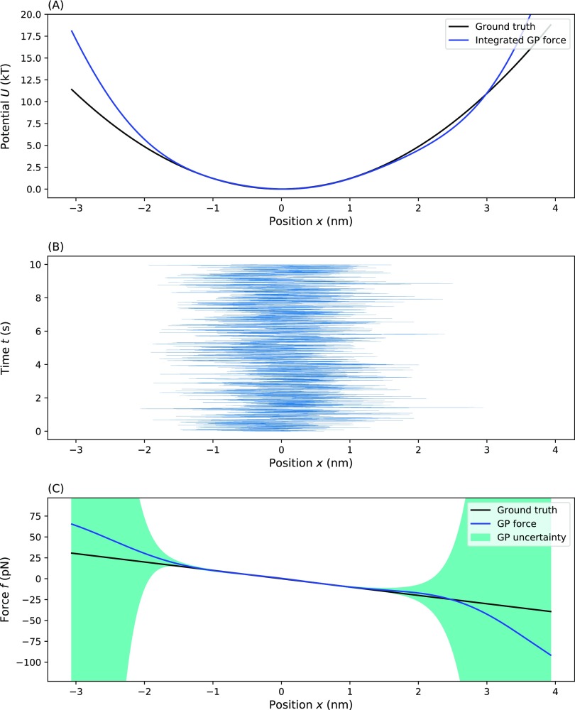
To demonstrate our method, we applied it to a synthetically generated time trace, consisting of N = 10⁴ data points, of a particle trapped in a harmonic potential well corresponding to the force f(x) = −Ax (Fig. 2). The values used in the simulation were ζ = 100 pg/μs, T = 300 K, and A = 10 pN/nm probed at τ = 1 µs. We looked for the effective force at 500 evenly spaced test points, ${\mathit{x}}_{1:M}^{*}$, around the spatial range of the time trace. The hyperparameters used that appear in Eq. (11) were σ = ατ($v$_max − $v$_min) and ℓ = (x_max − x_min)/2 with α = 1 pN/nm, where the subscripts max and min denote the maximum and minimum values from the trace. Briefly, here, our motivation for using these values is to set a length, ℓ, that correlates points over the spatial range covered in the time trace and yet still allows distant regions to be independent, and to set a prefactor, σ, which gives uncertainty proportional to the range of measured forces. The sensitivity of our method to the particular choice of hyperparameters is analyzed in the supplementary material.

FIG. 2.

Testing our method on a harmonic potential. This plot shows the inference of an effective force (and resulting effective potential) from a simple one-dimensional harmonic well test case: (a) the ground truth potential and our estimate obtained by integrating the MAP effective force estimate, (b) the time trace on which inference was performed, and (c) the ground truth force and the GP inferred effective force with uncertainty. For (a) and (c), the blue line represents the MAP estimate, the dark green shading represents a one standard deviation confidence interval, and the black line represents the ground truth. Parameters used for the simulation are ζ = 100 pg/μs, T = 300 K, τ = 1 µs, and f(x) = −Ax with A = pN/nm.

For simple forces lacking finer detail, the choice of hyperparameters is less critical especially as the number of data points, N, increases (see the supplementary material). Similarly, agreement of the predicted effective force with the ground truth is best when the effective force is close to zero (i.e., in regions of the effective potential where data points are more commonly sampled). As we look further out from the center where there are fewer data points, the uncertainty increases; however, the MAP estimate is still close to the ground truth. This is because the GP prior imposes a smoothness assumption set by the hyperparameters in Eq. (11), which favors maintaining the trend from the MAP estimate from better sampled regions, that is, regions with more data. In regions with no data, the uncertainty eventually grows to the prior value (determined by the first hyperparameter, σ) and the MAP estimate for f(·) eventually converges to the prior mean [f(·) = 0].

1. Varying the number of data points

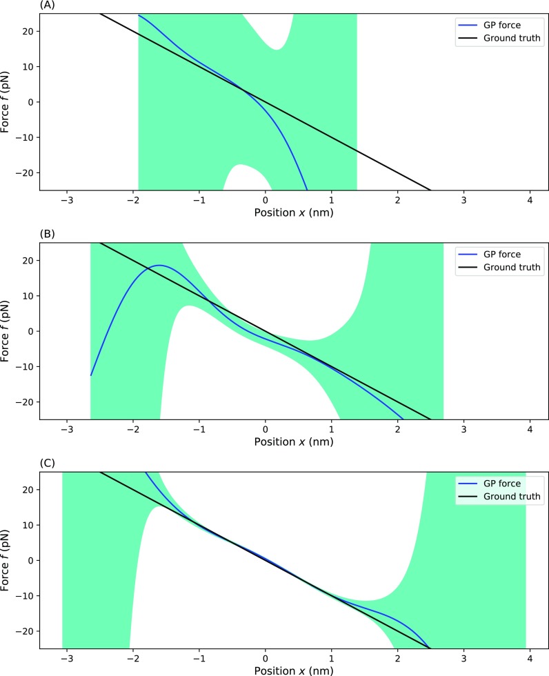
Previously, in Fig. 2, we looked at 10⁴ number of data points. Here, we characterize the quality of our force estimates as a function of the number of data points considered in the force estimate. Figure 3 shows the dependency of the prediction of the force as a function of an increase in the number of data points, N. Even for datasets as small as 100 points [Fig. 3(a)], the GP gives a reasonable shape for the inferred effective force. However, the uncertainty (as captured by the green confidence interval) remains high. As we increase the number of points to 1000 [Fig. 3(b)] and 10 000 [Fig. 3(c)] points, we see that the predicted effective force converges to the ground truth force in well-sampled regions with high uncertainty relegated to the undersampled regions.

FIG. 3.

Testing our method as a function of the number of data points available. Here, we show the effective force inferred from trajectories simulated for a particle trapped in a one dimensional harmonic well with a different number of data points: (a) 100 data points, (b) 1000 data points, and (c) 10 000 data points. For each panel, the blue line represents the MAP estimate, the dark green shading represents a one standard deviation confidence interval, and the black line represents the ground truth. Parameters used for the simulation are ζ = 100 pg/μs, T = 300 K, τ = 1 µs, and f(x) = −Ax with A = pN/nm.

2. Varying the stiffness

Next, to test the robustness of our method with respect to the stiffness, we applied our method to data simulated with different values of ζ/τ.

Re-writing our equation with a new parameter, h = ζ/τ called the stiffness,

$$h\left(x_{n+1}-x_n\right)=f\left(x_n\right)+r_n,$$ (20)

$$r_n\sim \mathbf{\text{Normal}}\left(\mathrm{0,2}hkT\right),$$ (21)

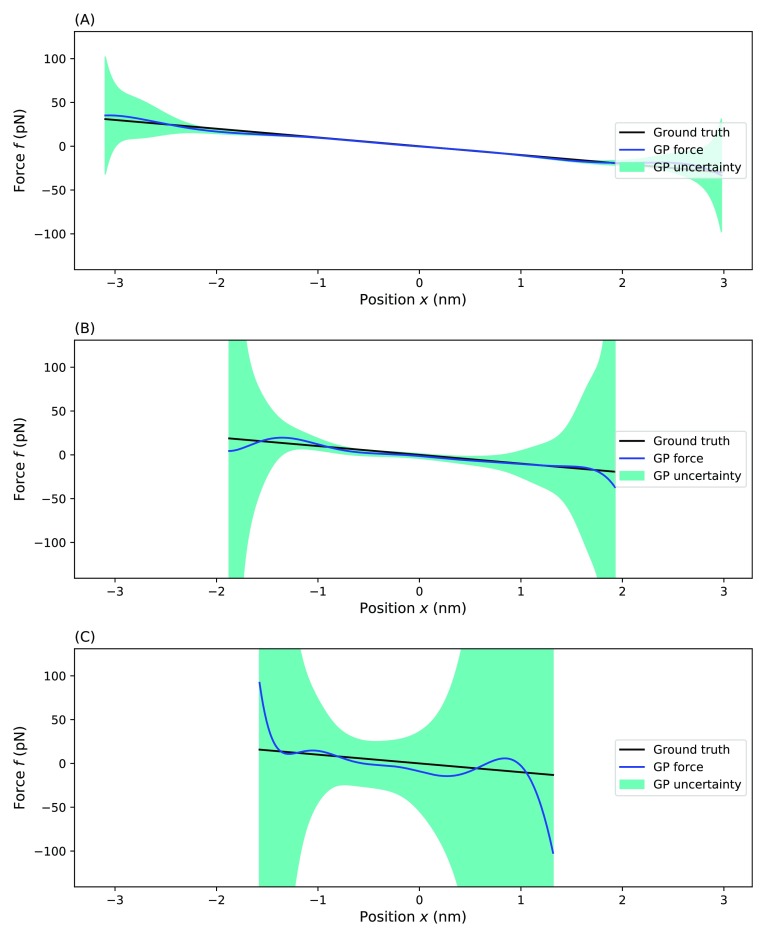
we see that varying the stiffness can be interpreted as changing the friction coefficient or the capture rate of the time trace, as ζ and τ always appear together in our model. The results are shown in Fig. 4.

FIG. 4.

Testing our method for a different stiffness. Here, we show the effective force inferred from 1000 point trajectories simulated for particles trapped in a one dimensional harmonic well using different choices of stiffness: (a) stiffness is h = 100 pg/μs, (b) stiffness is h = 1000 pg/μs, and (c) stiffness is h = 10 000 pg/μs. For each panel, the blue line represents the MAP estimate, the dark green shading represents a one standard deviation confidence interval, and the black line represents the ground truth. Parameters used for the simulation are T = 300 K and f(x) = −Ax with A = pN/nm.

For large values, the MAP estimate captures some of the trend, but the uncertainty remains large as thermal kicks at each time step dominate the dynamics. Frishman and Ronceray³⁹ described this in analogy to a signal to noise ratio. For small values of h, the prediction is, predictably, dramatically improved.

3. Double-well potential

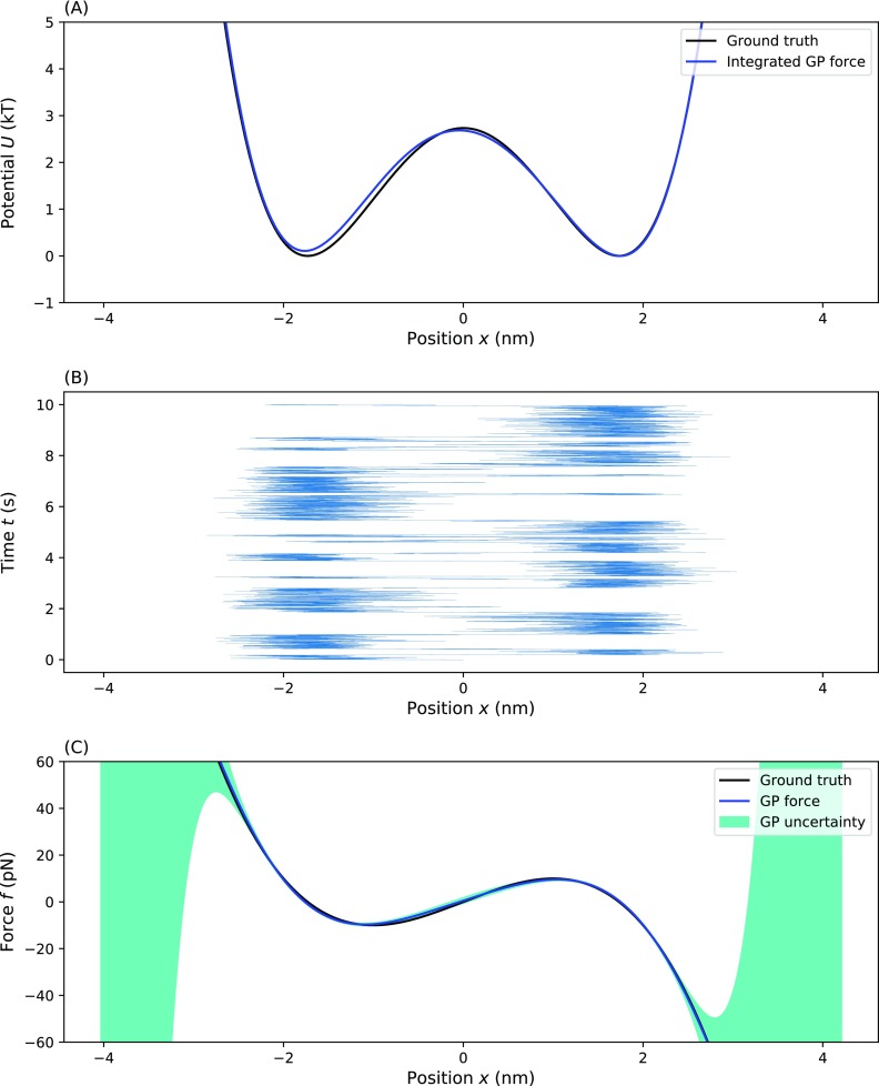
To further demonstrate our method on potentials of increasing complexity, we applied our method to a double well potential. As shown in Fig. 5, the shape of the learned effective force exactly matches the ground truth although there is a slight increase in the uncertainty of the middle region reflecting the undersampling in that region. The integrated learned force, as shown in Fig. 5(a), matches with the right potential well very closely, but for the left potential, the learned effective potential is slightly higher than the ground truth.

FIG. 5.

Testing our method on a double-well potential. Here, we show the effective force (and effective potential) inferred from the time trace of a particle diffusing within a double-well potential: (a) the ground truth and inferred effective potential, (b) the time trace on which the inference was performed, and (c) the ground truth force and the MAP estimate for the inferred effective force with uncertainty. For (a) and (c), the blue line represents the MAP estimate, the dark green shading represents a one standard deviation confidence interval, and the black line represents the ground truth. Parameters used for the simulation are ζ = 100 pg/μs, T = 300 K, τ = 1 µs, and f(x) = Ax⁴ − Bx² with A = 0.8 pN/nm⁴ and B = 7.5 pN/nm².

4. Multi-well potential

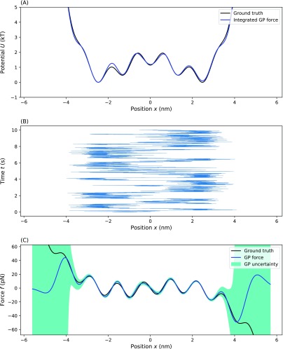
Next, we applied our method to a more complicated potential. We chose a rapidly spatially varying, multi-well potential to test how well our method can pick up on finer, often undersampled, potential details such as barriers. Here, we show how our method can be adapted to deal high frequency spatial variations in the potential. For example, we found that our method was able to pick up on the finer potential details when we decreased the length scale, ℓ, appearing as a hyperparameter to ℓ = (x_max − x_min)/10 so that correlations between distant points die out faster (see the supplementary material). The results are shown in Fig. 6. For a trace with N = 10⁴ time points, our method was able to find each of the wells reasonably well despite the potential’s greater complexity. The slight increase in uncertainty on the barriers suggests, as expected, that those regions are sampled less frequently. The integrated learned force matches well with the ground truth, as seen by comparing the learned effective potential to the ground truth [Fig. 6(a)] with only a slight overestimation of a barrier on the left side.

FIG. 6.

Testing our method on a multi-well potentials. Here, we show the effective force (and effective potential) inferred from the time trace of a particle diffusing within a multi-well potential: (a) the ground truth and inferred effective potential, (b) the time trace on which the inference was performed, and (c) the ground truth force and the MAP estimate for the inferred effective force with uncertainty. For (a) and (c), the blue line represents the MAP estimate, the dark green shading represents a one standard deviation confidence interval, and the black line represents the ground truth. Parameters used for the simulation are ζ = 100 pg/μs, T = 300 K, τ = 1 µs, and f(x) = Ax⁴ − Bx² − C cos(Dx) with A = 0.2 pN/nm⁴, B = 2 pN/nm², C = 2 pN, and D = 0.2 nm⁻¹.

5. Gibbs sampling for friction coefficient

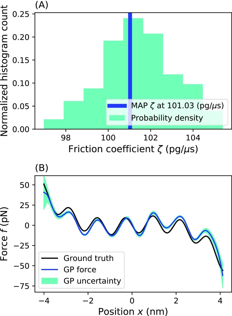
We used the Gibbs sampling scheme³⁷ to simultaneously sample a multi-well force and its corresponding friction coefficient from the time trace of position vs time. For our prior on ζ, we used a shape parameter α = 1 and a scale parameter β = 1000 pg/μs so that we could allow ζ to be sampled over a large range. By histogramming the sampled ζ⁽ⁱ⁾, we simulated the posterior on the friction coefficient [Fig. 7(a)]. Here, we see that the sampled values converged close to the true value. While not as good as the prediction with known friction coefficient (as also determining the friction coefficient demands more from the finite data available), we saw earlier, the prediction is still satisfactory. This demonstrates that the effective force can still be learned with an unknown friction coefficient.

FIG. 7.

Results of simultaneous force and friction coefficient determination using Gibbs sampling. This figure shows the inference of the force and friction coefficient using a Gibbs sampler. (a) A histogram of the sampled friction coefficients simulates the posterior on ζ. The highest probability sampled ζ was 101.03 pg/μs. The dark green represents the probability density. (b) The MAP force matches nicely with the ground truth force. Here, the blue line represents the MAP estimate, and the black line represents the ground truth. The dark green represents the one standard deviation confidence interval. Parameters used for the simulation are ζ = 100 pg/μs, T = 300 K, τ = 1 µs, and f(x) = Ax⁴ − Bx² − C cos(Dx) with A = 0.2 pN/nm⁴, B = 2 pN/nm², C = 2 pN, and D = 0.2 nm⁻¹.

B. Comparison with other methods

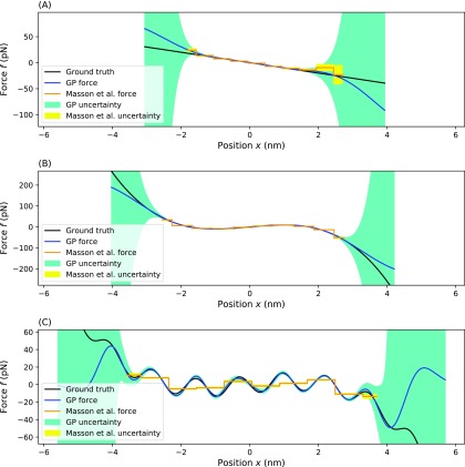
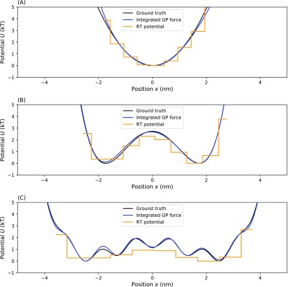
We compare our method described above to two previous methods to which we can compare most directly: that of Masson et al.,²⁷ which learns the effective force, and the residence time (RT) method,⁵ which learns the potential. Because the main proof of principle for our method is in learning the force, we compare all methods given a known friction coefficient selected to be ζ = 100 pg/μs. In order to compare our method to other methods, we use the following metric: how much data it take to converge to a force that is reasonably close to the ground truth. This will be shown in Figs. 8–10.

FIG. 8.

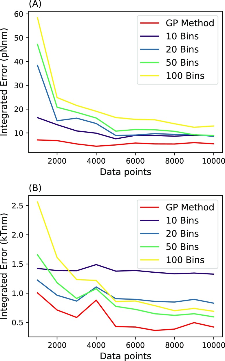
Error vs data points. Here, we compare the error of each method. Error was calculated by integrating the absolute value of the predicted effective force (a) or potential (b) subtracted from the ground truth force or potential over the range [−1 nm, 1 nm]. Different bin numbers of Masson et al. and residence time were compared. In (a), we compare the amount of data points it takes for our method and the Masson et al. method to converge to an accurate effective force field for the harmonic well. In (b), we compare the amount of data points it takes for our method and the RT method to converge to an accurate effective potential for the harmonic well. Parameters used for the simulation are ζ = 100 pg/μs, T = 300 K, τ = 1 µs, and f(x) = −Ax with A = pN/nm.

FIG. 9.

Comparison of our method with the Masson et al. method. In this figure, we compare our method to the Masson et al. method on three different effective force fields. The top compares inferences on the simplest, harmonic, potential (a). The middle compares inference on a double-well potential (b). The bottom compares inference on a multi-well potential (c). For each panel, the blue line represents the MAP estimate from our method, the dark green region represents the one standard deviation confidence interval for our estimate, the orange line represents the MAP estimate of the Masson et al. method, the yellow region represents the one standard deviation confidence interval of the Masson et al. method, and the black line represents the ground truth. Parameters for the simulation are the same as used in Secs. III A, III A 3, and III A 4.

FIG. 10.

Comparison of our method with residence time. In this figure, we compare our method to the residence time method on three different effective force fields. The top compares inferences on the simplest, harmonic, potential (a). The middle compares inference on a double-well potential (b). The bottom compares inference on a multi-well potential (c). For each panel, the blue line represents our MAP estimate, the orange line represents the residence time MAP estimate, and the black line represents the ground truth. Parameters used for the simulations are the same, as shown in Secs. III A, III A 3, and III A 4.

1. Masson et al.

We first compare to method of Masson et al.,²⁷ which follows a Bayesian strategy similar in spirit to ours. This method uses the same likelihood as in Eq. (9) but spatially bins the data into S equally sized bins and uses flat priors on the force in each bin instead of the GP prior of Eq. (12). This approach then finds a force and friction coefficient, which maximizes the posterior.²⁷ This method is optimized for simultaneously learning force and friction coefficient, but for simplified comparison, we hold ζ fixed. For known friction coefficient and one dimensional motion, this method reduces to averaging the measured force in each bin. This method predicts the effective force strength in bin s to be

$$f\left(x\right)=\frac{1}{C_s}\sum _{n:x_n\in s}\frac{\zeta }{\tau }\left(x_{n+1}-x_n\right),$$ (22)

where C_s is the number of times the position was measured in bin s. Bin size should be chosen so that each bin contains a sufficient number of data points to allow meaningful inference.²⁶ We found that 10 bins was optimal, but for completeness, when analyzing accuracy, we try many different bin numbers (Fig. 8).

Looking at Fig. 8(a), we see that our method converges to within a pre-specified error with fewer data points. The error was determined by numerically integrating the absolute value of the predicted effective force subtracted from the ground truth force over a range between −1 nm and +1 nm. We chose this range because it is the region with the most data and thus, the region in which the Masson et al. method best performs. For the Masson et al. method, a smaller bin size led to a smaller error. However, this effect emerged only after a large number of data points because for smaller bins, there are fewer data points per bin. Similarly, the method of Masson et al. also suffers in regions with few data points as this method averages the force from points within each bin. Outlier data points heavily influence effective forces inferred in these regions. On the right-hand side of the harmonic force [Fig. 9(a)], we see that a few outlier measurements dominate the inference in this region. For this reason, the method produces an incorrect predicted effective force. On the other hand, within our method, the smoothness assumption imposed by the GP prior prevents the prediction from being influenced by these points too heavily.

For the double-well potential [Fig. 9(b)], the Masson et al. method under-estimates the effective force in the steep parts of the effective potential. This is because the method averages all the points in the bin equally, regardless of location. Because the force in each bin is not spatially constant, the sides of each bin will have different forces. There inevitably are more points at the low force side of each bin than at the high force side, and so each bin is dominated by data points displaying a lower effective force. The GP prior avoids binning altogether and thus avoids this problem altogether.

2. Residence time

We also compared our method to the residence time (RT) analysis for finding the effective potential.⁴⁰ This method also bins space but totally ignores times. For each bin, s, this method assumes that under Boltzmann statistics, the expected number of times a particle is found in bin s after N measurements is given by

$$N_s=N{e}^{-U_s/kT}.$$ (23)

Solving for U_s, this method predicts the effective potential in bin s to be

$$U_s=-kT\ln \left(N_s/N\right).$$ (24)

For a harmonic potential, the RT method gives a good prediction [Fig. 10(a)]. For the more complex, multi-well, potential [Fig. 10(c)], the prediction by RT is not satisfactory. Here, the RT method underestimates the potential and does not capture all of the fine details. For the double-well potential force, while our method predicts an accurate force, it does slightly overestimate the potential in the left well. That is because our method is tailored for accurate effective force predictions and potential predictions are a post-processing step, which introduces additional (albeit small and bounded) errors due to integration (see the supplementary material).

IV. CONCLUSION

Learning effective forces is an important task as knowledge of appropriate forces allows us to develop reduced models of the dynamics of complex biological macromolecules.^19–24 Here, we developed a framework in which we inferred effective force profiles from time traces of position vs time for which positions may be undersampled. In order to learn both friction coefficient and forces simultaneously from the same dataset—and avoid binning or other pre-processing procedures that otherwise introduce artifacts—we developed a Gibbs sampling scheme and exploited Gaussian process priors over forces.

As such, our method simultaneously exploits every data point without binning or pre-processing and provides full Bayesian posterior over the prediction of the friction coefficient and force while placing minimal prior assumptions on the force profile.

A limitation of our method is its poor scalability. This is an inherent limitation of GP themselves, as these statistical tools naturally require the inversion of large matrices. The computations required to perform these inversions scale roughly as (N + M)³, where N, M are the number of data points and test points, respectively, and, as such, to do this for any datasets larger than roughly 50 000 data points requires around 100 gigabytes of memory. However, in the high data limit, as our method becomes more difficult to run or in the absence of high barriers in the potential, existing methods, such as the Masson et al. method and the residence time method, perform well, as errors due to binning become smaller with more data. Thus, our method supplements the existing methods to be used in the low data limits or when we anticipate poorly sampled regions of phase space. Moving forward, it is also worth noting that approximate inference for GP methods is under active development that may allow our method to be used in the high data limit.^41,42

Beyond computational improvements that are necessary for large scale applications, there are many ways to generalize the framework we proposed. In particular, at some computational cost, the form for the likelihood could be adapted to treat different models including measurement noise. Reminiscent of the hidden Markov model,^43,44 this may be achieved by adapting the Gibbs sampling scheme to learn the positions themselves hidden by the noise from the data.⁴ Furthermore, just as we placed a prior on the friction coefficient, we may also place a prior on the initial condition or even potentially treat more general (non-constant) friction coefficients.^14,15,45

Yet, another way to build off of our formulation is to generalize our analysis to multidimensional trajectories. Multidimensional datasets are common when combining single molecule measurements from force spectroscopy⁴⁶ and Förster resonance energy transfer.^3,4,47 To treat these datasets within our GP framework is straightforward as we would simply need to choose a kernel allowing two- or higher-dimensional inputs.²⁹

In conclusion, we have demonstrated a new method for finding the effective force field of an environment with minimal prior commitment to the form of the force field, exploiting every data point without binning or pre-processing, which can predict the force on the full posterior with credible intervals.

SUPPLEMENTARY MATERIAL

See the supplementary material for definitions of the probability distributions (Sec. A), post-processing to determine the potential from the force (Sec. B), an in-depth description of Bayes’ theorem and the Gaussian process prior (Sec. C), and explanation of the hyperparameter role in the inference (Sec. D).

AUTHOR’S CONTRIBUTIONS

J.S.B. analyzed data and developed analysis software; J.S.B., I.S., and S.P. conceived research; and S.P. oversaw all aspects of the projects.

REFERENCES

- 1.Espanol P. and Zuniga I., “Obtaining fully dynamic coarse-grained models from MD,” Phys. Chem. Chem. Phys. 13, 10538–10545 (2011). 10.1039/c0cp02826f [DOI] [PubMed] [Google Scholar]
- 2.Mardt A., Pasquali L., Wu H., and Noé F., “Vampnets for deep learning of molecular kinetics,” Nat. Commun. 9, 4443 (2018). 10.1038/s41467-018-06999-0 [DOI] [PMC free article] [PubMed] [Google Scholar]
- 3.Sgouralis I., Whitmore M., Lapidus L., Comstock M. J., and Pressé S., “Single molecule force spectroscopy at high data acquisition: A Bayesian nonparametric analysis,” J. Chem. Phys. 148, 123320 (2018). 10.1063/1.5008842 [DOI] [PubMed] [Google Scholar]
- 4.Jazani S., Sgouralis I., Shafraz O. M., Levitus M., Sivasankar S., and Pressé S., “An alternative framework for fluorescence correlation spectroscopy,” Nat. Commun. 10, 3662 (2019). 10.1038/s41467-019-11574-2 [DOI] [PMC free article] [PubMed] [Google Scholar]
- 5.Reif F., Fundamentals of Statistical and Thermal Physics (Waveland Press, 2009). [Google Scholar]
- 6.Schlick T., Molecular Modeling and Simulation: An Interdisciplinary Guide: An Interdisciplinary Guide (Springer Science & Business Media, 2010), Vol. 21. [Google Scholar]
- 7.Schaudinnus N., Lickert B., Biswas M., and Stock G., “Global Langevin model of multidimensional biomolecular dynamics,” J. Chem. Phys. 145, 184114 (2016). 10.1063/1.4967341 [DOI] [PubMed] [Google Scholar]
- 8.Micheletti C., Bussi G., and Laio A., “Optimal Langevin modeling of out-of-equilibrium molecular dynamics simulations,” J. Chem. Phys. 129, 074105 (2008). 10.1063/1.2969761 [DOI] [PubMed] [Google Scholar]
- 9.Zwanzig R., Nonequilibrium Statistical Mechanics (Oxford University Press, 2001). [Google Scholar]
- 10.Manzo C. and Garcia-Parajo M. F., “A review of progress in single particle tracking: From methods to biophysical insights,” Rep. Prog. Phys. 78, 124601 (2015). 10.1088/0034-4885/78/12/124601 [DOI] [PubMed] [Google Scholar]
- 11.Meijering E., Dzyubachyk O., and Smal I., “Methods for cell and particle tracking,” in Methods in Enzymology (Elsevier, 2012), Vol. 504, pp. 183–200. [DOI] [PubMed] [Google Scholar]
- 12.Sgouralis I. and Pressé S., “An introduction to infinite HMMs for single-molecule data analysis,” Biophys. J. 112, 2021–2029 (2017). 10.1016/j.bpj.2017.04.027 [DOI] [PMC free article] [PubMed] [Google Scholar]
- 13.Sgouralis I. and Pressé S., “ICON: An adaptation of infinite HMMs for time traces with drift,” Biophys. J. 112, 2117–2126 (2017). 10.1016/j.bpj.2017.04.009 [DOI] [PMC free article] [PubMed] [Google Scholar]
- 14.Pressé S., Peterson J., Lee J., Elms P., MacCallum J. L., Marqusee S., Bustamante C., and Dill K., “Single molecule conformational memory extraction: P5ab RNA hairpin,” J. Phys. Chem. B 118, 6597–6603 (2014). 10.1021/jp500611f [DOI] [PMC free article] [PubMed] [Google Scholar]
- 15.Pressé S., Lee J., and Dill K. A., “Extracting conformational memory from single-molecule kinetic data,” J. Phys. Chem. B 117, 495–502 (2013). 10.1021/jp309420u [DOI] [PMC free article] [PubMed] [Google Scholar]
- 16.Kusumi A., Sako Y., and Yamamoto M., “Confined lateral diffusion of membrane receptors as studied by single particle tracking (nanovid microscopy). Effects of calcium-induced differentiation in cultured epithelial cells,” Biophys. J. 65, 2021–2040 (1993). 10.1016/s0006-3495(93)81253-0 [DOI] [PMC free article] [PubMed] [Google Scholar]
- 17.Simson R., Sheets E. D., and Jacobson K., “Detection of temporary lateral confinement of membrane proteins using single-particle tracking analysis,” Biophys. J. 69, 989–993 (1995). 10.1016/s0006-3495(95)79972-6 [DOI] [PMC free article] [PubMed] [Google Scholar]
- 18.Welsher K. and Yang H., “Imaging the behavior of molecules in biological systems: Breaking the 3D speed barrier with 3D multi-resolution microscopy,” Faraday Discuss. 184, 359–379 (2015). 10.1039/c5fd00090d [DOI] [PubMed] [Google Scholar]
- 19.Wang J., Olsson S., Wehmeyer C., Pérez A., Charron N. E., De Fabritiis G., Noé F., and Clementi C., “Machine learning of coarse-grained molecular dynamics force fields,” ACS Cent. Sci. 5, 755 (2019). 10.1021/acscentsci.8b00913 [DOI] [PMC free article] [PubMed] [Google Scholar]
- 20.Chmiela S., Tkatchenko A., Sauceda H. E., Poltavsky I., Schütt K. T., and Müller K.-R., “Machine learning of accurate energy-conserving molecular force fields,” Sci. Adv. 3, e1603015 (2017). 10.1126/sciadv.1603015 [DOI] [PMC free article] [PubMed] [Google Scholar]
- 21.Kumar S., Rosenberg J. M., Bouzida D., Swendsen R. H., and Kollman P. A., “The weighted histogram analysis method for free-energy calculations on biomolecules. I. The method,” J. Comput. Chem. 13, 1011–1021 (1992). 10.1002/jcc.540130812 [DOI] [Google Scholar]
- 22.Foley T. T., Shell M. S., and Noid W. G., “The impact of resolution upon entropy and information in coarse-grained models,” J. Chem. Phys. 143, 243104 (2015). 10.1063/1.4929836 [DOI] [PubMed] [Google Scholar]
- 23.Izvekov S. and Voth G. A., “A multiscale coarse-graining method for biomolecular systems,” J. Phys. Chem. B 109, 2469–2473 (2005). 10.1021/jp044629q [DOI] [PubMed] [Google Scholar]
- 24.Marrink S. J., Risselada H. J., Yefimov S., Tieleman D. P., and De Vries A. H., “The martini force field: Coarse grained model for biomolecular simulations,” J. Phys. Chem. B 111, 7812–7824 (2007). 10.1021/jp071097f [DOI] [PubMed] [Google Scholar]
- 25.Straub J. E. and Thirumalai D., “Exploring the energy landscape in proteins,” Proc. Natl. Acad. Sci. U. S. A. 90, 809–813 (1993). 10.1073/pnas.90.3.809 [DOI] [PMC free article] [PubMed] [Google Scholar]
- 26.Tuerkcan S., Alexandrou A., and Masson J.-B., “A Bayesian inference scheme to extract diffusivity and potential fields from confined single-molecule trajectories,” Biophys. J. 102, 2288–2298 (2012). 10.1016/j.bpj.2012.01.063 [DOI] [PMC free article] [PubMed] [Google Scholar]
- 27.Masson J.-B., Casanova D., Türkcan S., Voisinne G., Popoff M.-R., Vergassola M., and Alexandrou A., “Inferring maps of forces inside cell membrane microdomains,” Phys. Rev. Lett. 102, 048103 (2009). 10.1103/physrevlett.102.048103 [DOI] [PubMed] [Google Scholar]
- 28.Lee A., Tsekouras K., Calderon C., Bustamante C., and Pressé S., “Unraveling the thousand word picture: An introduction to super-resolution data analysis,” Chem. Rev. 117, 7276–7330 (2017). 10.1021/acs.chemrev.6b00729 [DOI] [PMC free article] [PubMed] [Google Scholar]
- 29.Rasmussen C. E., “Gaussian processes in machine learning,” in Summer School on Machine Learning (Springer, 2003), pp. 63–71. [Google Scholar]
- 30.Gelman A., Carlin J. B., Stern H. S., Dunson D. B., Vehtari A., and Rubin D. B., Bayesian Data Analysis (Chapman and Hall/CRC, 2013). [Google Scholar]
- 31.Von Toussaint U., “Bayesian inference in physics,” Rev. Mod. Phys. 83, 943 (2011). 10.1103/revmodphys.83.943 [DOI] [Google Scholar]
- 32.Tavakoli M., Taylor J. N., Li C.-B., Komatsuzaki T., and Pressé S., “Single molecule data analysis: An introduction,” in Advances in Chemical Physics (John Wiley & Sons, Inc., 2017), pp. 205–305. 10.1002/9781119324560.ch4 [DOI] [Google Scholar]
- 33.Abraham M., Hess B., van der Spoel D., and Lindahl E., GROMACS user manual version 2018, 2018.
- 34.Petersen K. B. and Pedersen M. S., The Matrix Cookbook (Technical University of Denmark, 2012). [Google Scholar]
- 35.Bishop C. M., Pattern Recognition and Machine Learning (Springer-Verlag, 2006). [Google Scholar]
- 36.Do C. and Lee H., Gaussian processes, 2008.
- 37.Gilks W. R., Best N. G., and Tan K. K. C., “Adaptive rejection metropolis sampling within Gibbs sampling,” Appl. Stat. 44, 455–472 (1995). 10.2307/2986138 [DOI] [Google Scholar]
- 38.Robert C. and Casella G., Monte Carlo Statistical Methods (Springer Science & Business Media, 2013). [Google Scholar]
- 39.Frishman A. and Ronceray P., “Learning force fields from stochastic trajectories,” Phys. Rev. X (to be published); arXiv:1809.09650 (2018).https://journals.aps.org/prx/accepted/10077K6aO441f00873804e05f49d6599b66979640 [Google Scholar]
- 40.Florin E.-L., Pralle A., Stelzer E., and Hörber J., “Photonic force microscope calibration by thermal noise analysis,” Appl. Phys. A: Mater. Sci. Process. 66, S75–S78 (1998). 10.1007/s003390051103 [DOI] [Google Scholar]
- 41.Nemeth C., Sherlock C. et al. , “Merging MCMC subposteriors through Gaussian-process approximations,” Bayesian Anal. 13, 507–530 (2018). 10.1214/17-ba1063 [DOI] [Google Scholar]
- 42.Titsias M. K., Lawrence N., and Rattray M., “Markov chain Monte Carlo algorithms for Gaussian processes,” in Inference and Estimation in Probabilistic Time-Series Models (University of Cambridge, 2008), Vol. 9. [Google Scholar]
- 43.Beal M. J., Ghahramani Z., and Rasmussen C. E., “The infinite hidden Markov model,” in Advances in Neural Information Processing Systems (Neural Information Processing Systems Foundation, Inc., 2002), pp. 577–584. [Google Scholar]
- 44.Rabiner L. R. and Juang B.-H., “An introduction to hidden Markov models,” IEEE ASSP Mag. 3, 4–16 (1986). 10.1109/massp.1986.1165342 [DOI] [Google Scholar]
- 45.Satija R., Das A., and Makarov D. E., “Transition path times reveal memory effects and anomalous diffusion in the dynamics of protein folding,” J. Chem. Phys. 147, 152707 (2017). 10.1063/1.4993228 [DOI] [PubMed] [Google Scholar]
- 46.Hummer G. and Szabo A., “Free energy reconstruction from nonequilibrium single-molecule pulling experiments,” Proc. Natl. Acad. Sci. U. S. A. 98, 3658–3661 (2001). 10.1073/pnas.071034098 [DOI] [PMC free article] [PubMed] [Google Scholar]
- 47.Sgouralis I., Madaan S., Djutanta F., Kha R., Hariadi R. F., and Pressé S., “A bayesian nonparametric approach to single molecule Förster resonance energy transfer,” J. Phys. Chem. B 123, 675–688 (2018). 10.1021/acs.jpcb.8b09752 [DOI] [PMC free article] [PubMed] [Google Scholar]
Associated Data
This section collects any data citations, data availability statements, or supplementary materials included in this article.
Supplementary Materials