

Abstract
Neuromelanin-sensitive MRI (NM-MRI) provides a noninvasive measure of the content of neuromelanin (NM), a product of dopamine metabolism that accumulates with age in dopamine neurons of the substantia nigra (SN). NM-MRI has been validated as a measure of both dopamine neuron loss, with applications in neurodegenerative disease, and dopamine function, with applications in psychiatric disease. Furthermore, a voxelwise-analysis approach has been validated to resolve substructures, such as the ventral tegmental area (VTA), within midbrain dopaminergic nuclei thought to have distinct anatomical targets and functional roles. NM-MRI is thus a promising tool that could have diverse research and clinical applications to noninvasively interrogate in vivo the dopamine system in neuropsychiatric illness. Although a test-retest reliability study by Langley et al. using the standard NM-MRI protocol recently reported high reliability, a systematic and comprehensive investigation of the performance of the method for various acquisition parameters and preprocessing methods has not been conducted. In particular, most previous studies used relatively thick MRI slices (~3 mm), compared to the typical in-plane resolution (~0.5 mm) and to the height of the SN (~15 mm), to overcome technical limitations such as specific absorption rate and signal-to-noise ratio, at the cost of partial-volume effects. Here, we evaluated the effect of various acquisition and preprocessing parameters on the strength and test-retest reliability of the NM-MRI signal to determine optimized protocols for both region-of-interest (including whole SN-VTA complex and atlas-defined dopaminergic nuclei) and voxelwise measures. Namely, we determined a combination of parameters that optimizes the strength and reliability of the NM-MRI signal, including acquisition time, slice-thickness, spatial-normalization software, and degree of spatial smoothing. Using a newly developed, detailed acquisition protocol, across two scans separated by 13 days on average, we obtained intra-class correlation values indicating excellent reliability and high contrast, which could be achieved with a different set of parameters depending on the measures of interest and experimental constraints such as acquisition time. Based on this, we provide detailed guidelines covering acquisition through analysis and recommendations for performing NM-MRI experiments with high quality and reproducibility. This work provides a foundation for the optimization and standardization of NM-MRI, a promising MRI approach with growing applications throughout clinical and basic neuroscience.
Keywords: Neuromelanin, Test-retest, Substantia nigra, Ventral tegmental area, NM-MRI, Voxelwise analysis
1. Introduction
Neuromelanin (NM) is an insoluble dark pigment that consists of melanin, proteins, lipids, and metal ions (Zecca et al., 2008). Neurons containing NM are present in specific brain regions of the human central nervous system with particularly high concentrations found in the dopaminergic neurons of the substantia nigra (SN) and noradrenergic neurons of the locus coeruleus (LC) (Zecca et al., 1996; Zucca et al., 2014). NM is synthesized by iron-dependent oxidation of dopamine, norepinephrine, and other catecholamines in the cytosol, to semi-quinones and quinones (Sulzer and Zecca, 1999). While initially present in the cytosol, NM accumulates within cytoplasmic organelles via macroautophagy that results in the undegradable material being taken into autophagic vacuoles (Sulzer et al., 2000). These vacuoles then fuse with lysosomes and other autophagic vacuoles containing lipid and protein components to form the final NM-containing organelles (Zucca et al., 2014). These organelles contain NM pigment along with metals, abundant lipid bodies, and protein matrix (Zecca et al., 2000; Zucca et al., 2018). This process was shown to be driven by excess cytosolic catecholamines, such as that resulting from L-DOPA exposure, that are not accumulated in synaptic vesicles and can be inhibited by treatment with the iron chelator desferrioxamine (Cebrián et al., 2014; Sulzer et al., 2000). NM-containing organelles first appear in humans between 2 and 3 years of age (Cowen, 1986) and gradually accumulate with age (Zecca et al., 2008; Zucca et al., 2018).
The paramagnetic nature of the NM-iron complexes within the NM-containing organelles (Zecca et al., 1996, 2004) enables them to be noninvasively imaged using magnetic resonance imaging (MRI) (Cassidy et al., 2019; Sasaki et al., 2006; Sulzer et al., 2018; Trujillo et al., 2017). NM-sensitive MRI (NM-MRI) produces hyperintense signals in neuromelanin-containing regions such as the SN and LC due to the short longitudinal relaxation time (T1) of the NM-complexes and saturation of the surrounding white matter (WM) by either direct magnetization transfer (MT) pulses (Chen et al., 2014) or indirect MT effects (Sasaki et al., 2006) (see Trujillo et al. for a detailed investigation of NM-MRI contrast mechanisms (Trujillo et al., 2017)). While most previous NM-MRI studies have used indirect MT effects, images with direct MT pulses achieve greater sensitivity (Langley et al., 2015; Schwarz et al., 2013) and were recently shown to be directly related to NM concentration (Cassidy et al., 2019). NM-MRI has also been validated as a measure of dopaminergic neuron loss in the SN (Kitao et al., 2013) and several studies have shown that this method can capture the well-known loss of NM-containing neurons in the SN of individuals with Parkinson’s disease (Sulzer et al., 2018). More recently, NM-MRI was validated as a marker of dopamine function, with the NM-MRI signal in the SN demonstrating a significant relationship to Positron emission tomography (PET) measures of dopamine release capacity in the striatum (Cassidy et al., 2019). Furthermore, a voxelwise-analysis approach was validated to resolve substructures within dopaminergic nuclei thought to have distinct anatomical targets and functional roles (Cassidy et al., 2019; Haber et al., 1995; Roeper, 2013; Weinstein et al., 2017). This voxelwise approach may thus allow for a more anatomically precise interrogation of specific midbrain circuits encompassing subregions within the SN or small dopaminergic nuclei such as the ventral tegmental area (VTA), which may in turn increase the accuracy of NM-MRI markers for clinical or mechanistic research. For example, voxelwise NM-MRI may facilitate investigations into the specific subregions within the SN-VTA complex projecting to the head of the caudate, which are of particular relevance in the study of psychosis (Weinstein et al., 2017), or help capture the known topography of SN neuronal loss in Parkinson’s disease (Cassidy et al., 2019; Damier et al., 1999; Fearnley and Lees, 1991). An additional benefit of the voxelwise analysis is avoiding the circularity that can incur when defining ROIs based on the NM-MRI images that are then used to read out the signal in those same regions. Most previous studies have used the high signal region in the NM-MRI images to define the SN region-of-interest (ROI) that is used for further analysis. While this may be appropriate if the goal of the study is to measure the volume of the SN, it can be problematic for analysis of the contrast ratio (CNR) because the selected ROI is biased towards high CNR voxels.
NM-MRI can be a promising tool with diverse research and clinical applications to noninvasively interrogate in vivo the dopamine system. However, this is critically dependent on a thorough investigation of the performance of the method for various acquisition parameters and preprocessing methods. In particular, most previous studies used relatively thick MRI slices (~3 mm) (Langley et al., 2017; Sasaki et al., 2008; Schwarz et al., 2011), compared to the in-plane resolution (~0.5 mm) and to the height of the SN (~15 mm) (Pauli et al., 2018), to overcome technical limitations such as specific absorption rate and signal-to-noise ratio (SNR), at the cost of partial-volume effects. Additionally, previous studies acquired multiple measurements that were subsequently averaged to improve the SNR of the technique with the expense of increased scanning time. Although time in the MRI is expensive and should be minimized to improve patient compliance, a detailed investigation into how many measurements are necessary for robust NM-MRI has not been reported. A recent study reported high reproducibility for ROI analysis (Langley et al., 2017). However, this study did not provide a detailed description of NM-MRI volume placement and the two scans were obtained within a single session, although subjects were removed and repositioned in-between scans.
Here, we evaluate the effect of various acquisition and preprocessing parameters on the strength and test-retest reliability of the NM-MRI signal to determine optimized protocols for both ROI and voxelwise measures. Three new NM-MRI sequences with slice-thickness of 1.5 mm, 2 mm, and 3 mm were compared to the literature-standard sequence with 3 mm slice-thickness (Cassidy et al., 2019; Chen et al., 2014). Using our step-by-step acquisition protocol, across the two acquired scans we obtained intra-class correlation coefficient (ICC) values indicating excellent reliability and high CNR, which could be achieved with a different set of parameters depending on the measures of interest and experimental constraints such as acquisition time. A detailed analysis of the CNR and ICC provide evidence for the optimal spatial-normalization software, number of measurements (acquisition time), slice-thickness, and spatial smoothing. Based on this, we provide detailed guidelines covering acquisition through analysis and recommendations for performing NM-MRI experiments with high quality and reproducibility.
2. Methods
2.1. Participants
10 healthy subjects underwent 2 MRI exams (test and re-test) on a 3T Prisma MRI (Siemens, Erlangen, Germany) using a 64-channel head coil. The test-retest scans were separated by a minimum of 2 days. Inclusion criteria were: age between 18 and 65 years and no MRI contraindications. Exclusion criteria were: history of neurological or psychiatric diseases, pregnancy or nursing, and inability to provide written consent. This study was approved by the Stony Brook University Institutional Review Board and written informed consent was obtained from all subjects.
2.2. Magnetic resonance imaging
A T1-weighted (T1w) image was acquired for processing of the NM-MRI image using a 3D magnetization prepared rapid acquisition gradient echo (MPRAGE) sequence with the following parameters: spatial resolution = 0.8× 0.8 × 0.8 mm3; field-of-view (FOV) = 166 × 240 × 256 mm3; echo time (TE) = 2.24 ms; repetition time (TR) = 2,400 ms; inversion time (TI) = 1060 ms; flip angle = 8°; in-plane acceleration, GRAPPA = 2 (Griswold et al., 2002); bandwidth = 210 Hz/pixel. A T2-weighted (T2w) image was acquired for processing of the NM-MRI image using a 3D sampling perfection with application-optimized contrasts by using flip angle evolution (SPACE) sequence with the following parameters: spatial resolution = 0.8 × 0.8 × 0.8 mm3; FOV = 166 × 240 × 256 mm3; TE = 564 ms; TR = 3,200 ms; echo spacing = 3.86 ms; echo train duration = 1,166 ms; variable flip angle (T2 var mode); in-plane acceleration = 2; bandwidth = 744 Hz/pixel. NM-MRI images were acquired using 4 different 2D gradient recalled echo sequences with magnetization transfer contrast (2D GRE-MTC) (Chen et al., 2014). The following parameters were consistent across the 4 2D GRE-MT sequences: in-plane resolution = 0.4 × 0.4 mm2; FOV = 165 × 220 mm2; flip angle = 40°; slice gap = 0 mm; bandwidth = 390 Hz/pixel; MT frequency offset = 1.2 kHz; MT pulse duration = 10 ms; MT flip angle = 300°; partial k-space coverage of MT pulse as described by Chen et al. (2014). The partial k-space coverage MT pulses were applied in a trapezoidal fashion as described by Parker et al. (1995) with ramp-up and ramp-down coverage of 20% and plateau coverage of 40%. Other 2D GRE-MTC sequence parameters that differed across the 4 sequences are listed in Table 1. The order of the 4 NM-MRI sequences was randomized across all subjects and sessions.
Table 1.
2D GRE-MTC sequence parameters used for NM-MRI.
| Sequence | TE (ms) | TR (ms) | Slice-Thickness (mm) | Number of Slices | Number of Acquisitions | Acquisition Time (minutes:s) | In-Plane Acceleration |
|---|---|---|---|---|---|---|---|
| NM-1.5 mm | 4.11 | 444 | 1.5 | 16 | 11 | 10:51 | 2 |
| NM-2 mm | 3.61 | 321 | 2 | 12 | 15 | 10:42 | 2 |
| NM-3 mm | 3.61 | 214 | 3 | 8 | 23 | 10:56 | 2 |
| NM-3 mm Standard | 3.87 | 273 | 3 | 10 | 10 | 11:02 | None |
2.3. Neuromelanin-MRI placement protocol
Given the limited coverage of the NM-MRI protocol in the inferior-superior direction (~30 mm), a detailed NM-MRI volume placement procedure based on distinct anatomical landmarks was developed to improve within-subject and across-subject repeatability. The placement protocol makes use of the sagittal, coronal, and axial 3D T1w images. Furthermore, the coronal and axial images were reformatted along the anterior commissure-posterior commissure (AC-PC) line. The following is the step-by-step procedure used for NM-MRI volume placement:
Identification of the sagittal image showing the greatest separation between the midbrain and thalamus (Fig. 1A).
Using the sagittal image from the end of Step 1, finding the coronal plane that identifies the most anterior aspect of the midbrain (Fig. 1B).
Using the coronal image from the end of Step 2, finding the axial plane that identifies the inferior aspect of the third ventricle (Fig. 1C and 1D).
Setting the superior boundary of the NM-MRI volume to be 3 mm superior to the axial plane from the end of Step 3 (Fig. 1E).
Fig. 1.

Illustration of the step-by-step procedure for placement of the NM-MRI volume. Yellow lines indicate the position of slices used for placing the volume. (A) Sagittal image showing the greatest separation between the midbrain and thalamus. (B) Coronal plane that identifies the most anterior aspect of the midbrain on the image from A. (C) Axial plane that identifies the inferior aspect of the third ventricle on the image of the coronal plane from B. (D) Location of the axial plane from C identified on the image from A. (E) The axial plane denoting the superior boundary of the NM-MRI volume. This axial plane is the axial plane from D shifted superiorly 3 mm.
Because the NM-MRI volume was placed relative to the axial and coronal images reformatted along the AC-PC line, the final angle of the NM-MRI volume is along the AC-PC line. Additionally, the NM-MRI volume should be angled parallel to the brain midline in the axial and coronal planes. Although some previous NM-MRI studies have oriented the NM-MRI volume perpendicular to the floor of the 4th ventricle, we chose to orient it along the AC-PC line to improve reproducibility. Because there is no unique plane that runs perpendicular to the SN-VTA complex and the exact plane perpendicular to the floor of the 4th ventricle is somewhat ambiguous, we chose a plane that is easily identified across subjects and commonly used in MRI. An example of the final placement from a representative subject is shown in Fig. 2 along with a NM-MRI image from each of the 4 NM-MRI sequences.
Fig. 2.
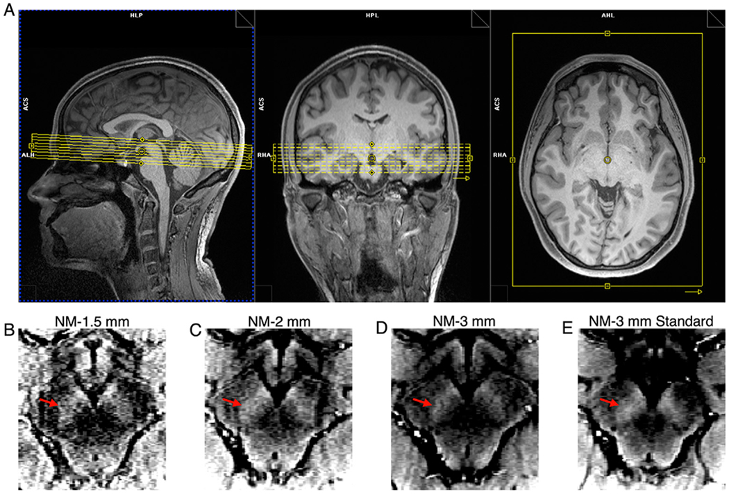
NM-MRI volume placement and NM-MRI images from the 4 NM-MRI sequences tested in this study from a representative subject. (A) Final NM-MRI volume placement. (B–E) Raw signal in axial slices at approximately the same level of the midbrain for each NM-MRI sequence, after motion correction and averaging: (B) NM-1.5 mm, (C) NM-2 mm, (D) NM-3 mm, and (E) NM-3 mm Standard. The intensity scales for the NM-MRI images were set such that the ratio between the lower bound and upper bound was 25%. Red arrows on B – E denote the left SN-VTA complex.
2.4. Neuromelanin-MRI preprocessing
The NM-MRI preprocessing pipeline was written in Matlab (Math-Works, Natick, MA) using SPM12 (Penny et al., 2011). The steps of the pipeline were as follows: 1) The intra-sequence acquisitions were realigned to the first acquisition to correct for inter-acquisition motion using ‘SPM-Realign’ to perform 6-parameter rigid-body registration; 2) The motion corrected NM-MRI images were subsequently averaged; 3) The average NM-MRI images were then coregistered to the T1w image using ‘SPM-Coregister’ to perform 6-parameter rigid-body registration; 4) The average NM-MRI images were resliced to the resolution of the T1w image (0.8 × 0.8 × 0.8 mm3) using ‘SPM-Reslice’; 5) The T1w image was spatially normalized to a standard MNI template using 4 different software: ANTs (Avants et al., 2008, 2009), FSL (Andersson et al., 2007; Jenkinson et al., 2012), SPM12’s Unified Segmentation (referred to as SPM12 throughout) (Ashburner and Friston, 2005; Penny et al., 2011) and SPM12’s DARTEL (referred to as DARTEL throughout) (Ashburner, 2007; Penny et al., 2011). The warping parameters to normalize the T1w image to the MNI template were then applied to the coregistered NM-MRI images using the respective software. The resampled resolution of the spatially normalized NM-MRI images was 1 mm, isotropic. Additionally, the spatially normalized NM-MRI images were spatially smoothed using 3D Gaussian kernels with full-width-at-half-maximum (FWHM) of 0 mm (no smoothing), 1 mm, 2 mm, and 3 mm. All analyses using manually traced ROIs used the standard 1 mm spatial smoothing. All ROI-analysis results used 0 mm of spatial smoothing and all voxelwise-analysis results used 1 mm of spatial smoothing unless otherwise specified.
2.5. Neuromelanin-MRI analysis
The ROIs used in this study included a manually traced mask of the SN-VTA complex defined from a previous study (Cassidy et al., 2019) and ROIs of the dopaminergic nuclei within the SN-VTA complex: SN pars compacta (SNc), SN pars reticulata (SNr), ventral tegmental area (VTA), and parabrachial pigmented nucleus (PBP) as defined from a high-resolution probabilistic atlas (Pauli et al., 2018). Details regarding the creation of the manually traced mask can be found in (Cassidy et al., 2019). Briefly, a template NM-MRI image was generated by averaging the spatially normalized NM-MRI images from 40 individuals (20 individuals with schizophrenia and 20 healthy controls). The hyperintense region depicting the SN-VTA complex was manually traced on this NM-MRI template image. This tracing was purposefully overinclusive to better ensure that all voxels in all possible subjects’ SN-VTA complex would be included. The neighboring hypointense region depicting the CC was also manually traced. Fig. 3 shows the ROIs overlaid on a template NM image. This mask was used to maintain consistency with the only NM-MRI study that validated the NM-MRI signal directly against NM concentration in brain tissue (Cassidy et al., 2019). Additionally, all of the probabilistic masks of dopaminergic nuclei are contained within the manually traced mask. Although the investigated NM-MRI sequences were not optimized for locus coeruleus (LC) imaging, preliminary analyses for probabilistic LC masks are presented in the Supplement.
Fig. 3.

Spatial normalization and anatomical masks for analysis of NM-MRI images. (A) Average NM-MRI image created by averaging the spatially normalized NM-MRI images from 10 individuals in MNI space. Note the high signal intensity in the SN-VTA complex. (B) Masks for the SN-VTA complex (yellow voxels) and the CC (pink voxels) reference region (used in the calculation of CNR) are overlaid onto the template in A. These anatomical masks were made by manual tracing on a NM-MRI template from a previous study (Cassidy et al., 2019). Note the hyper-intensity along the edge of the midbrain and that the SN-VTA-complex mask does include the anterior medial edge, which is also not included in the probabilistic masks in D. (C) The same average NM-MRI image from A but different slices. (D) Probabilistic masks for the VTA, SNr, SNc, and PBP as defined from a high-resolution probabilistic atlas (Pauli et al., 2018) overlaid onto the template in C. The color scaling for probabilistic masks goes from P = 0.5 (darkest) to P = 0.8 (lightest). Red arrows in A and C denote the left SN-VTA complex.
The NM-MRI contrast ratio (CNR) at each voxel in the NM-MRI image was calculated as the percent signal difference in NM-MRI signal intensity at a given voxel (IV) from the signal intensity in the crus cerebri (ICC), a region of white matter tracts known to have minimal NM content (Cassidy et al., 2019), as CNRV = {[IV − mode(ICC)]/mode(ICC)}*100. Where mode(ICC) was calculated for each participant from a kernel-smoothing-function fit of a histogram of all voxels in the CC mask. This method was found to be more robust to outlier voxels in the CC mask (e.g., due to edge artifacts) relative to computing the mean or median (Cassidy et al., 2019).
2.6. Statistical analysis
Two-way mixed, single score intraclass correlation coefficient [ICC(3,1)] (Shrout and Fleiss, 1979) were used to assess the test-retest reliability of NM-MRI. This ICC is a measure of consistency between the first and second measurements that does not penalize consistent changes across all subjects (e.g., if the retest CNR is consistently higher than the test CNR for all subjects). The maximum ICC is 1, indicating perfect reliability, ICC over 0.75 indicates “excellent” reliability, ICC between 0.75 and 0.6 indicates “good” reliability, ICC between 0.6 and 0.4 indicates “fair” reliability, and ICC under 0.4 indicates “poor” reliability (Cicchetti, 1994). ICC(3,1) values were calculated for three conditions: the average CNR within a given ROI (1 ICC value per ROI; ICCROI); the across-subject voxelwise CNR (1 ICC value per voxel; ICCASV); the within-subject voxelwise CNR (1 ICC value per subject; ICCWSV). ICCROI provides a measure of the reliability of the average CNR within an ROI across all subjects, thus providing a measure of the reliability of the ROI-analysis approach. ICCASV provides a measure of the reliability of CNRV at each voxel within an ROI across all subjects, thus providing a measure of the reliability of the voxelwise-analysis approach. ICCWSV provides a measure of the reliability of the spatial pattern of CNRV across voxels within each of the subjects individually, which provides a complementary measure of reliability of the voxelwise-analysis approach.
The relationship between CNRV and ICCASV was assessed using Spearman correlation. Multiple linear regression analysis predicting ICCASV of voxels within the manually traced mask as a function of their coordinates in x (absolute distance from the midline), y, and z directions was used to evaluate the predictive value of anatomical position on ICCASV. Wilcoxon signed rank tests were used to compare the CNRV and ICCASV between different magnitudes of spatial smoothing.
3. Results
3.1. Demographics
The test-retest MRI exams were separated by 13 ± 13 (mean ± standard deviation) days on average with a median of 8 days, minimum of 2 days, and maximum of 38 days. Of the 10 subjects, 4 were male and 6 were female; 4 were Caucasian and 6 were Asian; 9 were right-handed and 1 was left-handed. The average age was 27 ± 5 years (mean ± standard deviation). None of the subjects reported current cigarette smoking or recreational drug use.
3.2. Required acquisition time
Plots of ICCROI and CNRROI within the manually traced mask as a function of acquisition time for each of the NM-MRI sequences and spatial normalization software are shown in Fig. 4. In general, all NM-MRI sequences and spatial normalization software achieved excellent test-retest reliability within 3 min of acquisition time and CNRROI was not affected by acquisition time. The NM-1.5 mm sequence had the highest CNRROI for all spatial normalization software while the NM-3 mm sequence had the lowest. Table 2 lists the ICCROI and the 25th percentile, median, and 75th percentile of and CNRROI values shown in Fig. 4 for 3 min of acquisition time.
Fig. 4.

ICCROI (top row) and CNRROI (bottom row) within the manually traced mask of the SN-VTA complex (Fig. 3B) as a function of acquisition time. Data points denote the median and error bars indicate the 25th and 75th percentiles.
Table 2.
ICCROI and CNRROI for each NM-MRI sequence and spatial normalization software. ICCROI and CNRROI values are from within the manually traced mask of the SN-VTA complex (Fig. 3B) and for CNRROI are listed as 25th percentile, median, 75th percentile.
| Sequence | Spatial Normalization Software | ICCROI | CNRROI |
|---|---|---|---|
| NM-1.5 mm | ANTs | 0.95 | 15.1, 21.8, 23.1 |
| FSL | 0.93 | 13.5, 20.3, 21.4 | |
| SPM12 | 0.96 | 16.0, 23.3, 25.5 | |
| DARTEL | 0.92 | 14.1, 21.3, 22.9 | |
| NM-2 mm | ANTs | 0.97 | 13.1, 18.6, 21.5 |
| FSL | 0.97 | 11.6, 17.7, 19.8 | |
| SPM12 | 0.98 | 13.5, 20.7, 23.1 | |
| DARTEL | 0.94 | 12.6, 17.1, 20.1 | |
| NM-3 mm | ANTs | 0.95 | 9.1, 15.3, 16.7 |
| FSL | 0.95 | 8.2, 14.7, 15.9 | |
| SPM12 | 0.89 | 14.8, 16.3, 19.6 | |
| DARTEL | 0.72 | 4.6, 11.4, 15.6 | |
| NM-3 mm Standard | ANTs | 0.98 | 10.5, 18.0, 19.3 |
| FSL | 0.98 | 9.5, 16.8, 18.4 | |
| SPM12 | 0.95 | 12.4, 19.8, 20.6 | |
| DARTEL | 0.89 | 11.4, 15.5, 17.1 |
Plots of the ICCASV, ICCWSV, and CNRV within the manually traced mask as a function of acquisition time for each of the NM-MRI sequences and spatial normalization software are shown in Fig. 5. In general, all spatial normalization software and NM-MRI sequences except for NM-3 mm achieved excellent test-retest reliability within 6 min of acquisition time and CNRV was not affected by acquisition time. The NM-1.5 mm sequence had the highest CNRV for all spatial normalization software while the NM-3 mm sequence had the lowest.
Fig. 5.

ICCASV (top row), ICCWSV (middle row), and CNRV (bottom row) of voxels within the manually traced mask of the SN-VTA complex (Fig. 3B) as a function of acquisition time. Data points denote the median and error bars indicate the 25th and 75th percentiles.
3.3. Choice of NM-MRI sequence
Scatterplots of the ICCASV and CNRV of each voxel within the manually traced mask for each of the NM-MRI sequences and spatial normalization software are shown in Fig. 6. Table 3 lists the 25th percentile, median, and 75th percentile of ICCASV and CNRV values and the correlation between ICCASV and CNRV shown in Fig. 6. The NM-1.5 mm sequence consistently showed the highest CNRV, greatest spread in CNRV, lowest correlation between CNRV and ICCASV, and high ICCASV across all spatial normalization software. Because the NM-1.5 mm sequence demonstrated the best performance, further optimization was performed for this sequence and the following sections only use data from this sequence.
Fig. 6.

Scatterplots of ICCASV and CNRV for each of the NM-MRI sequences and spatial normalization software. Each data point represents one voxel within the manually traced mask of the SN-VTA complex (Fig. 3B). The solid lines indicate the linear fit of the relationship between ICCASV and CNRV.
Table 3.
ICCASV, CNRV, and Spearman’s rho of their relationship for each NM-MRI sequence and spatial normalization software. ICCASV and CNRV values are from within the manually traced mask of the SN-VTA complex (Fig. 3B) and are listed as 25th percentile, median, 75th percentile. Spearman’s rho values represent the relationship between ICCASV and CNRV of voxels within the manually traced mask.
| Sequence | Spatial Normalization Software | ICCASV | CNRV | ρ |
|---|---|---|---|---|
| NM-1.5 mm | ANTs | 0.86, 0.91, 0.94 | 13.2, 17.3, 21.6 | 0.26 |
| FSL | 0.82, 0.88, 0.92 | 12.6, 16.2, 19.7 | 0.22 | |
| SPM12 | 0.77, 0.86, 0.91 | 16.7, 20.4, 23.8 | 0.26 | |
| DARTEL | 0.85, 0.89, 0.92 | 15.3, 18.8, 22.3 | 0.25 | |
| NM-2 mm | ANTs | 0.87, 0.92, 0.95 | 12.7, 16.1, 19.3 | 0.37 |
| FSL | 0.73, 0.90, 0.95 | 11.5, 14.4, 17.5 | 0.49 | |
| SPM12 | 0.65, 0.81, 0.90 | 14.5, 17.9, 21.1 | 0.35 | |
| DARTEL | 0.81, 0.88, 0.92 | 14.3, 17.3, 19.9 | 0.26 | |
| NM-3 mm | ANTs | 0.21, 0.77, 0.93 | 7.9, 10.6, 13.4 | 0.42 |
| FSL | 0.51, 0.83, 0.94 | 5.9, 9.5, 12.2 | 0.33 | |
| SPM12 | −0.04, 0.24, 0.91 | 9.9, 12.4, 14.9 | 0.27 | |
| DARTEL | 0.32, 0.80, 0.86 | 7.3, 10.2, 12.9 | 0.54 | |
| NM-3 mm Standard | ANTs | 0.84, 0.95, 0.97 | 11.3, 14.6, 17.1 | 0.30 |
| FSL | 0.86, 0.94, 0.96 | 11.3, 13.7, 15.9 | 0.35 | |
| SPM12 | 0.70, 0.84, 0.89 | 13.2, 16.2, 18.6 | 0.42 | |
| DARTEL | 0.85, 0.91, 0.94 | 10.5, 13.2, 15.3 | 0.47 |
3.4. Choice of spatial normalization software
To determine which spatial normalization software should be used for voxelwise-analysis of NM-MRI data, multiple linear regression analysis predicting ICCASV of voxels within the manually traced mask as a function of their coordinates in x (absolute distance from the midline), y, and z directions was used. The rationale here is that, with an optimal method, the ICC should be highest and homogeneous across voxels such that the voxel’s anatomical location should not predict its associated ICC value. This analysis showed that ANTs achieved the best performance in that anatomical position was least predictive of ICCASV and it provided the highest ICCASV (Fig. 7). This result was consistent with a previous study where ANTs outperformed 13 other spatial-normalization algorithms (Klein et al., 2009).
Fig. 7.

(A) Predictive value (R2) of anatomical position on ICCASV of voxels within the manually traced mask of the SN-VTA complex (Fig. 3B) for NM-1.5 mm sequence and each of the spatial normalization software. Data points denote the median and error bars indicate the 25th and 75th percentiles. (B) Histogram of ICCASV of voxels within the manually traced mask for NM-1.5 mm sequence and ANTs spatial normalization software, which is the best performing method as per A. (C) Histogram of ICCASV of voxels within the manually traced mask for NM-1.5 mm sequence and SPM12 spatial normalization software, which is the worst performing method as per A. Yellow denotes excellent reliability (ICC over 0.75), orange denotes good reliability (ICC between 0.75 and 0.6), red denotes fair reliability (ICC between 0.6 and 0.4), and burgundy denotes poor reliability (ICC under 0.4).
3.5. Effect of spatial smoothing
A plot showing the relationship of ICCASV and CNRV of voxels within the manually traced mask at 4 levels of spatial smoothing is shown in Fig. 8. Greater amounts of spatial smoothing lead to significantly lower CNRV and significantly higher ICCASV (Wilcoxon signed rank test, P < 0.001 for all after correction for multiple comparisons). Relative to the one-lower degree of spatial smoothing (e.g., 2 mm vs 1 mm), spatial smoothing with 1 mm FWHM achieved the greatest increase in ICCASV and lowest decrease in CNRV, 0.03 and −0.09, respectively. Although there was still a significant difference in ICCASV and CNRV between spatial smoothing with FWHM of 0 mm and 1 mm, the minimal difference in CNRV and overall improvement in the robustness of voxelwise analysis and spatial normalization in particular, support the use of spatial smoothing with 1 mm FWHM.
Fig. 8.

The effect of spatial smoothing on ICCASV and CNRV of voxels within the manually traced mask of the SN-VTA complex (Fig. 3B) for different degrees of spatial smoothing. Data points denote the median and error bars show the 25th and 75th percentiles.
3.6. Analyses using probabilistic atlas of dopaminergic nuclei
Using a recent high-resolution probabilistic atlas that identified the dopaminergic nuclei (Pauli et al., 2018), we evaluated the feasibility of obtaining reliable measures of NM-MRI signal in these nuclei. Such measures would be valuable for basic and clinical neuroscience, particularly for the VTA, given its importance for reward learning (Montague et al., 1996; Schultz, 1998; Ungless et al., 2004) and affective processing (Depue and Collins, 1999; Fields et al., 2007). Plots of the ICCROI and CNRROI within the probabilistic masks as a function of acquisition time for the NM-1.5 mm sequence and ANTs spatial normalization software and various probability cutoffs are shown in Fig. 9. In general, excellent test-retest reliability was achieved for all nuclei and all probability cutoff values within 6 min of acquisition time. Similar to CNR in the manually traced mask, the CNRROI was not affected by acquisition time. The highest CNR was consistently observed in the SNr and SNc, then the PBP, and the lowest CNR in the VTA.
Fig. 9.

ICCROI (top row) and CNRROI (bottom row) within the probabilistic masks of the dopaminergic nuclei (Fig. 3D) with different probability cutoffs (0.5, 0.6, 0.7, and 0.8) as a function of acquisition time. Data points denote the median and error bars indicate the 25th and 75th percentiles.
Having established the ability to reliably measure NM-MRI within dopaminergic nuclei, we then investigated how distinct the NM-MRI signal within each nuclei is. The dopaminergic nuclei are believed to have distinct anatomical projections and functional roles, so independently measuring signals from these nuclei would allow for investigation into these distinct anatomical circuits and functions. Although the nuclei are anatomically distinct, the potential for cross-contamination of the NM-MRI signal exists due to partial volume effects and spatial blurring due to MRI acquisition and the spatial normalization procedure. The independence of CNRROI values measured within the individual dopaminergic nuclei was assessed by nonparametric Spearman’s correlation (Fig. 10). Overall, CNR was highly correlated across the four nuclei, particularly for ROI definitions based on a probability cutoff of P = 0.5.
Fig. 10.

Correlations and histograms of the CNRROI values within the 4 dopaminergic nuclei (Fig. 3D) for the lowest (P = 0.5) and highest (P = 0.8) probability cutoffs. The value within each correlation plot is Spearman’s rho.
4. Discussion
We present here a detailed description of a volume placement protocol for NM-MRI and use a test-retest study design to quantitatively derive recommendations for NM-MRI sequence parameters and preprocessing methods to achieve reproducible NM-MRI for ROI and voxelwise analyses. Additionally, by using a high-resolution probabilistic atlas, we were able to determine the reproducibility of NM-MRI measurements in specific dopaminergic nuclei within the SN-VTA complex. Overall, excellent reproducibility was observed in all ROIs investigated and for voxels within the ROIs. Based on our results, we recommend acquiring at least 6 min of data for voxelwise analysis or dopaminergic-nuclei-ROI analysis and at least 3 min of data for standard SN-VTA-complex analysis. We also recommend acquiring NM-MRI data with 1.5 mm slice-thickness, using ANTs for spatial normalization, and performing spatial smoothing with a 1 mm FWHM 3D Gaussian kernel for voxelwise analysis and no spatial smoothing for ROI analysis (especially for analysis of dopaminergic nuclei).
The goal of this paper was to provide detailed guidelines covering acquisition through analysis and recommendations for performing NM-MRI experiments with high quality and reproducibility. The main metric used to determine the recommendations was ICC. The high ICC values observed in our test-retest study suggest that NM-MRI using 2D GRE-MT sequences achieve excellent reproducibility across several acquisition and preprocessing combinations. This is in agreement with a previous report that observed an ICCROI value of 0.81 for SN in 11 healthy subjects (Langley et al., 2017). Surprisingly the present study observed higher ICCROI values (~0.92) even though our study used a template-defined SN-VTA-complex mask and the two MRI scans were separated by 13 ± 13 days instead of using a subject-specific semi--automated thresholding method for SN mask generation (Chen et al., 2014) and having test-retest scans within a single session in one day (in which subjects were removed from the scanner after the first session, repositioned on the table, and scanned again). The improved ICCROI observed in our study could be explained by the rigor of the NM-MRI volume placement protocol, which makes use of easy to identify anatomical landmarks to improve the reproducibility of volume placement across sessions. The study by Langley et al. focused on ROI measures and did not measure voxelwise ICC, so our study also extends this previous work in suggesting that voxelwise CNR measures can be obtained reliably. Another recent study measured ICCASV in 8 healthy subjects and 8 patients with schizophrenia, also with both MRI sessions on the same day (~1 h apart) (Cassidy et al., 2019). That study observed a median ICCASV value of 0.64 and an ICCROI value of 0.96. The higher ICCASV observed in the present study could be due to the inclusion of only healthy subjects as well as the detailed volume placement protocol.
In addition to ICC values, we also used the strength of the NM-MRI signal (CNR) and the range of CNR values. Because correlation-based approaches are common for voxelwise analysis, a greater range in CNR values within the SN-VTA complex will provide greater statistical power. Another important factor in our analysis was the relationship between CNR and ICC. To make sure that voxelwise-analysis effects are not driven solely by high (or low) CNR voxels due to lower measurement noise in those voxels, it is important to have homogeneously high ICC values independent of CNR. Our recommended ANTs-based method applied to NM-MRI data with 1.5 mm slice-thickness maximizes this independence.
This study is the first NM-MRI study to measure CNR in nuclei within the SN-VTA complex. This was facilitated by making use of a publicly available high-resolution probabilistic atlas (Pauli et al., 2018). We demonstrated that the NM-MRI signal within the nuclei is highly reproducible with ~6 min of data. Overall, we observed the highest CNR in the SNc and SNr, followed by the PBP, then the VTA. This is consistent with reports of higher degree of NM pigmentation in the SN than the VTA (Hirsch et al., 1988; Liang et al., 2004). However, we observed that the NM-MRI signal was highly correlated across nuclei. This finding may suggest that NM-MRI may only provide a measure of the general function of the dopamine system and is not specific to nuclei with distinct anatomy and function. While this may be true, our study included a limited number of subjects. Additionally, it is possible that the different functional domains of the dopamine system are highly correlated in healthy subjects and small errors in the realignment and spatial normalization processes could cause signal from different nuclei becoming mixed. These concerns could be partially mitigated through the use of a voxelwise analysis (Cassidy et al., 2019). A future study should be conducted to investigate variability in specific functional domains of the dopamine system to determine if NM-MRI is capable of independently assessing dopamine functions more closely related to each of the nuclei.
This study tested 2 NM-MRI sequences with 3 mm slice-thickness: NM-3 mm and NM-3 mm Standard. The main difference between these two NM-MRI sequences was the use of in-plane acceleration, the number of slices, the TE, and the TR. These parameters were changed relative to the literature standard protocol (i.e. NM-3 mm Standard) to accommodate the increased number of slices required for similar coverage in the higher resolution sequences (i.e. NM-1.5 mm and NM-2 mm). Although the higher resolution sequences did not seem to be affected, increased noise due to in-plane acceleration could have caused the lower reproducibility observed for the NM-3 mm sequence compared to the NM-3 mm Standard sequence (Robson et al., 2008). An alternative explanation is that the reduced number of slices results in reduced performance of the realignment and coregistration steps (resulting from less anatomical information for the algorithms to work with) leading to reduced reproducibility. All images were manually inspected at each step and no obvious errors occurred but small-scale deviations in the preprocessing could impact the reproducibility. Future studies are needed to better understand the effect of TE and TR on the reproducibility of the NM-MRI signal.
This work provides a foundation for several applications in both basic and clinical neuroscience. The high reliability of NM-MRI observed is this study provides strong evidence for NM-MRI as a reliable noninvasive tool to investigate the role of the dopaminergic system in vivo. This includes the study of reward related behavior (Schultz, 2007) and investigation of dopaminergic abnormalities in addiction (Kelley and Berridge, 2002; Koob et al., 1998), Parkinson’s disease (Fahn and Sulzer, 2004; Sulzer et al., 2018; Sulzer and Surmeier, 2013), depression (Dunlop and Nemeroff, 2007; Nestler and Carlezon Jr, 2006), and schizophrenia (Abi-Dargham et al., 2000; Davis et al., 1991; Laruelle et al., 1996; Weinstein et al., 2017). The potential for achieving highly reliable NM-MRI supports its continued use as a research tool throughout various applications, which in past work have included research in Parkinson’s disease (Aiba et al.; Cassidy et al., 2019; Hatano et al., 2017; Huddleston et al., 2017; Isaias et al., 2016; Kitao et al., 2013; Matsuura et al., 2013; Ohtsuka et al., 2014; Ohtsuka et al., 2013; Sasaki et al., 2006; Wang et al., 2019; Wang et al., 2018; Xing et al., 2018) and schizophrenia (Cassidy et al., 2019; Shibata et al., 2008; Watanabe et al., 2014; Yamashita et al., 2016), among others (Xing et al., 2018). Future studies may follow our guidelines or build upon them to obtain robust NM-MRI measures that are conducive to improved standardization across sites and studies, features that may be particularly relevant in biomarker development (Abi-Dargham and Horga, 2016).
The ability to acquire highly reproducible NM-MRI measurements for ROI-analysis with a 3-min acquisition opens the possibility of applications to clinical populations that may not have been previously possible due to prohibitively long acquisition times. While the mechanisms of NM-MRI contrast are not fully understood and its specificity in measuring NM concentration or dopamine neuron loss requires further investigation, our results suggest that this technique may provide a reliable tool for the development of neuropsychiatric biomarkers.
Limitations of the present study include not conducting an exhaustive search of MRI acquisition parameters (e.g. TR, TE) or MT parameters (e.g. flip angle, offset). Such a search would have made the present study untenable, so we focused on what we perceived as the most critical acquisition parameter: slice-thickness. Additionally, as the contrast mechanisms of NM-MRI signal are better understood (Trujillo et al., 2017), numerical simulations could be performed to optimize several acquisition parameters including TE, TR, and MT parameters. Another limitation was the inclusion of only relatively young and healthy subjects. As such, the ICC values in patients (e.g. psychosis, Parkinson’s) could be lower due to reduced compliance in the MRI, however increased range of CNR values in patients could result in higher ICC values.
5. Conclusions
We have empirically determined that highly reproducible NM-MRI can be achieved with at least 6 min of NM-MRI data for voxelwise analysis or dopaminergic-nuclei ROI analysis, and at least 3 min of NM-MRI data for ROI analysis. Additionally, we recommend using 1.5 mm slice-thickness, ANTs spatial normalization software, and spatial smoothing with 1 mm FWHM 3D Gaussian kernel. This work provides a foundation for the optimization and standardization of NM-MRI, a promising MRI approach with growing applications throughout basic and clinical neuroscience.
Supplementary Material
Acknowledgments
The authors would like to thank Drs. Xiaoping Hu and Jason Langley for consultation with implementing the partial k-space MT sequence. Pilot funding for MRI scanner time was provided by the SCAN Center at Stony Brook University. G.H. received funding from the NIMH (R01-MH114965, R01-MH117323).
Footnotes
Data and code availability
The code and the data used to produce the results reported in the manuscript are available from the corresponding author upon reasonable request.
Declaration of competing interest
The authors declare no conflicts of interest.
Appendix A. Supplementary data
Supplementary data to this article can be found online at https://doi.org/10.1016/j.neuroimage.2019.116457.
References
- Abi-Dargham A, Horga G, 2016. The search for imaging biomarkers in psychiatric disorders. Nat. Med 22, 1248. [DOI] [PubMed] [Google Scholar]
- Abi-Dargham A, Rodenhiser J, Printz D, Zea-Ponce Y, Gil R, Kegeles LS, Weiss R, Cooper TB, Mann JJ, Van Heertum RL, Gorman JM, Laruelle M, 2000. Increased baseline occupancy of D-2 receptors by dopamine in schizophrenia. Proc. Natl. Acad. Sci. U. S. A 97, 8104–8109. [DOI] [PMC free article] [PubMed] [Google Scholar]
- Aiba Y, Sakakibara R, Tsuyusaki Y, Oki T, Ogata T, Tateno F, Terada H, 2019. Neuromelanin-sensitive MRI in the differential diagnosis of elderly white matter lesion from Parkinson’s disease. Neurol. Clin. Neurosci 7, 322–325. 10.1111/ncn3.12320. [DOI] [Google Scholar]
- Andersson JL, Jenkinson M, Smith S, 2007. Non-linear Registration Aka Spatial Normalisation FMRIB Technial Report TR07JA2. FMRIB Analysis Group of the University of, Oxford. [Google Scholar]
- Ashburner J, 2007. A fast diffeomorphic image registration algorithm. Neuroimage 38, 95–113. [DOI] [PubMed] [Google Scholar]
- Ashburner J, Friston KJ, 2005. Unified segmentation. Neuroimage 26, 839–851. [DOI] [PubMed] [Google Scholar]
- Avants BB, Epstein CL, Grossman M, Gee JC, 2008. Symmetric diffeomorphic image registration with cross-correlation: evaluating automated labeling of elderly and neurodegenerative brain. Med. Image Anal 12, 26–41. [DOI] [PMC free article] [PubMed] [Google Scholar]
- Avants BB, Tustison N, Song G, 2009. Advanced normalization tools (ANTS). Insight j 2, 1–35. [Google Scholar]
- Cassidy CM, Zucca FA, Girgis RR, Baker SC, Weinstein JJ, Sharp ME, Bellei C, Valmadre A, Vanegas N, Kegeles LS, Brucato G, Jung Kang U, Sulzer D, Zecca L, Abi-Dargham A, Horga G, 2019. Neuromelanin-sensitive MRI as a noninvasive proxy measure of dopamine function in the human brain. Proc. Natl. Acad. Sci 116, 5108–5117. [DOI] [PMC free article] [PubMed] [Google Scholar]
- Cebrián C, Zucca FA, Mauri P, Steinbeck JA, Studer L, Scherzer CR, Kanter E, Budhu S, Mandelbaum J, Vonsattel JP, 2014. MHC-I expression renders catecholaminergic neurons susceptible to T-cell-mediated degeneration. Nat. Commun 5, 3633. [DOI] [PMC free article] [PubMed] [Google Scholar]
- Chen X, Huddleston DE, Langley J, Ahn S, Barnum CJ, Factor SA, Levey AI, Hu X, 2014. Simultaneous imaging of locus coeruleus and substantia nigra with a quantitative neuromelanin MRI approach. Magn. Reson. Imag 32, 1301–1306. [DOI] [PubMed] [Google Scholar]
- Cicchetti DV, 1994. Guidelines, criteria, and rules of thumb for evaluating normed and standardized assessment instruments in psychology. Psychol. Assess 6, 284. [Google Scholar]
- Cowen D, 1986. The melanoneurons of the human cerebellum (nucleus pigmentosus cerebellaris) and homologues in the monkey. J. Neuropathol. Exp. Neurol 45, 205–221. [PubMed] [Google Scholar]
- Damier P, Hirsch E, Agid Y, Graybiel A, 1999. The substantia nigra of the human brain: II. Patterns of loss of dopamine-containing neurons in Parkinson’s disease. Brain 122, 1437–1448. [DOI] [PubMed] [Google Scholar]
- Davis KL, Kahn RS, Ko G, Davidson M, 1991. Dopamine in schizophrenia - a review and reconceptualization. Am. J. Psychiatry 148, 1474–1486. [DOI] [PubMed] [Google Scholar]
- Depue RA, Collins PF, 1999. Neurobiology of the structure of personality: dopamine, facilitation of incentive motivation, and extraversion. Behav. Brain Sci 22, 491–517. [DOI] [PubMed] [Google Scholar]
- Dunlop BW, Nemeroff CB, 2007. The role of dopamine in the pathophysiology of depression. Arch. Gen. Psychiatr 64, 327–337. [DOI] [PubMed] [Google Scholar]
- Fahn S, Sulzer D, 2004. Neurodegeneration and neuroprotection in Parkinson disease. NeuroRx 1, 139–154. [DOI] [PMC free article] [PubMed] [Google Scholar]
- Fearnley JM, Lees AJ, 1991. Ageing and Parkinson’s disease: substantia nigra regional selectivity. Brain 114, 2283–2301. [DOI] [PubMed] [Google Scholar]
- Fields HL, Hjelmstad GO, Margolis EB, Nicola SM, 2007. Ventral tegmental area neurons in learned appetitive behavior and positive reinforcement. Annu. Rev. Neurosci 30, 289–316. [DOI] [PubMed] [Google Scholar]
- Griswold MA, Jakob PM, Heidemann RM, Nittka M, Jellus V, Wang J, Kiefer B, Haase A, 2002. Generalized autocalibrating partially parallel acquisitions (GRAPPA). Magn. Reson. Med 47, 1202–1210. [DOI] [PubMed] [Google Scholar]
- Haber S, Ryoo H, Cox C, Lu W, 1995. Subsets of midbrain dopaminergic neurons in monkeys are distinguished by different levels of mRNA for the dopamine transporter: comparison with the mRNA for the D2 receptor, tyrosine hydroxylase and calbindin immunoreactivity. J. Comp. Neurol 362, 400–410. [DOI] [PubMed] [Google Scholar]
- Hatano T, Okuzumi A, Kamagata K, Daida K, Taniguchi D, Hori M, Yoshino H, Aoki S, Hattori N, 2017. Neuromelanin MRI is useful for monitoring motor complications in Parkinson’s and PARK2 disease. J. Neural Transm 124, 407–415. [DOI] [PubMed] [Google Scholar]
- Hirsch E, Graybiel AM, Agid YA, 1988. Melanized dopaminergic neurons are differentially susceptible to degeneration in Parkinson’s disease. Nature 334, 345. [DOI] [PubMed] [Google Scholar]
- Huddleston DE, Langley J, Sedlacik J, Boelmans K, Factor SA, Hu XP, 2017. In vivo detection of lateral-ventral tier nigral degeneration in Parkinson’s disease. Hum. Brain Mapp 38, 2627–2634. [DOI] [PMC free article] [PubMed] [Google Scholar]
- Isaias IU, Trujillo P, Summers P, Marotta G, Mainardi L, Pezzoli G, Zecca L, Costa A, 2016. Neuromelanin imaging and dopaminergic loss in Parkinson’s disease. Front. Aging Neurosci 8, 196. [DOI] [PMC free article] [PubMed] [Google Scholar]
- Jenkinson M, Beckmann CF, Behrens TE, Woolrich MW, Smith SM, 2012. FSL. NeuroImage 62, 782–790. [DOI] [PubMed] [Google Scholar]
- Kelley AE, Berridge KC, 2002. The neuroscience of natural rewards: relevance to addictive drugs. J. Neurosci 22, 3306–3311. [DOI] [PMC free article] [PubMed] [Google Scholar]
- Kitao S, Matsusue E, Fujii S, Miyoshi F, Kaminou T, Kato S, Ito H, Ogawa T, 2013. Correlation between pathology and neuromelanin MR imaging in Parkinson’ s disease and dementia with Lewy bodies. Neuroradiology 55, 947–953. [DOI] [PubMed] [Google Scholar]
- Klein A, Andersson J, Ardekani BA, Ashburner J, Avants B, Chiang MC, Christensen GE, Collins DL, Gee J, Hellier P, Song JH, Jenkinson M, Lepage C, Rueckert D, Thompson P, Vercauteren T, Woods RP, Mann JJ, Parsey RV, 2009. Evaluation of 14 nonlinear deformation algorithms applied to human brain MRI registration. Neuroimage 46, 786–802. [DOI] [PMC free article] [PubMed] [Google Scholar]
- Koob GF, Sanna PP, Bloom FE, 1998. Neuroscience of addiction. Neuron 21, 467–476. [DOI] [PubMed] [Google Scholar]
- Langley J, Huddleston DE, Chen X, Sedlacik J, Zachariah N, Hu X, 2015. A multicontrast approach for comprehensive imaging of substantia nigra. Neuroimage 112, 7–13. [DOI] [PMC free article] [PubMed] [Google Scholar]
- Langley J, Huddleston DE, Liu CJ, Hu X, 2017. Reproducibility of locus coeruleus and substantia nigra imaging with neuromelanin sensitive MRI. Magn. Reson. Mater. Phys. Biol. Med 30, 121–125. [DOI] [PubMed] [Google Scholar]
- Laruelle M, Abi-Dargham A, vanDyck CH, Gil R, Dsouza CD, Erdos J, McCance E, Rosenblatt W, Fingado C, Zoghbi SS, Baldwin RM, Seibyl JP, Krystal JH, Charney DS, Innis RB, 1996. Single photon emission computerized tomography imaging of amphetamine-induced dopamine release in drug-free schizophrenic subjects. Proc. Natl. Acad. Sci. U. S. A 93, 9235–9240. [DOI] [PMC free article] [PubMed] [Google Scholar]
- Liang CL, Nelson O, Yazdani U, Pasbakhsh P, German DC, 2004. Inverse relationship between the contents of neuromelanin pigment and the vesicular monoamine transporter-2: human midbrain dopamine neurons. J. Comp. Neurol 473, 97–106. [DOI] [PubMed] [Google Scholar]
- Matsuura K, Maeda M, Yata K, Ichiba Y, Yamaguchi T, Kanamaru K, Tomimoto H, 2013. Neuromelanin magnetic resonance imaging in Parkinson’s disease and multiple system atrophy. Eur. Neurol 70, 70–77. [DOI] [PubMed] [Google Scholar]
- Montague PR, Dayan P, Sejnowski TJ, 1996. A framework for mesencephalic dopamine systems based on predictive Hebbian learning. J. Neurosci 16, 1936–1947. [DOI] [PMC free article] [PubMed] [Google Scholar]
- Nestler EJ, Carlezon WA Jr., 2006. The mesolimbic dopamine reward circuit in depression. Biol. Psychiatry 59, 1151–1159. [DOI] [PubMed] [Google Scholar]
- Ohtsuka C, Sasaki M, Konno K, Kato K, Takahashi J, Yamashita F, Terayama Y, 2014. Differentiation of early-stage parkinsonisms using neuromelanin-sensitive magnetic resonance imaging. Park. Relat. Disord 20, 755–760. [DOI] [PubMed] [Google Scholar]
- Ohtsuka C, Sasaki M, Konno K, Koide M, Kato K, Takahashi J, Takahashi S, Kudo K, Yamashita F, Terayama Y, 2013. Changes in substantia nigra and locus coeruleus in patients with early-stage Parkinson’s disease using neuromelanin-sensitive MR imaging. Neurosci. Lett 541, 93–98. [DOI] [PubMed] [Google Scholar]
- Parker DL, Buswell HR, Goodrich KC, Alexander AL, Keck N, Tsuruda JS, 1995. The application of magnetization transfer to MR angiography with reduced total power. Magn. Reson. Med 34, 283–286. [DOI] [PubMed] [Google Scholar]
- Pauli WM, Nili AN, Tyszka JM, 2018. A high-resolution probabilistic in vivo atlas of human subcortical brain nuclei. Scientific data 5, 180063. [DOI] [PMC free article] [PubMed] [Google Scholar]
- Penny WD, Friston KJ, Ashburner JT, Kiebel SJ, Nichols TE, 2011. Statistical Parametric Mapping: the Analysis of Functional Brain Images. Elsevier. [Google Scholar]
- Robson PM, Grant AK, Madhuranthakam AJ, Lattanzi R, Sodickson DK, McKenzie CA, 2008. Comprehensive quantification of signal-to-noise ratio and g-factor for image-based and k-space-based parallel imaging reconstructions. Magn. Reson. Med 60, 895–907. [DOI] [PMC free article] [PubMed] [Google Scholar]
- Roeper J, 2013. Dissecting the diversity of midbrain dopamine neurons. Trends Neurosci. 36, 336–342. [DOI] [PubMed] [Google Scholar]
- Sasaki M, Shibata E, Kudo K, Tohyama K, 2008. Neuromelanin-sensitive MRI. Clin. Neuroradiol 18, 147–153. [Google Scholar]
- Sasaki M, Shibata E, Tohyama K, Takahashi J, Otsuka K, Tsuchiya K, Takahashi S, Ehara S, Terayama Y, Sakai A, 2006. Neuromelanin magnetic resonance imaging of locus ceruleus and substantia nigra in Parkinson’s disease. Neuroreport 17, 1215–1218. [DOI] [PubMed] [Google Scholar]
- Schultz W, 1998. Predictive reward signal of dopamine neurons. J. Neurophysiol 80, 1–27. [DOI] [PubMed] [Google Scholar]
- Schultz W, 2007. Behavioral dopamine signals. Trends Neurosci. 30, 203–210. [DOI] [PubMed] [Google Scholar]
- Schwarz S, Bajaj N, Morgan P, Reid S, Gowland P, Auer D, 2013. Magnetisation transfer contrast to enhance detection of neuromelanin loss at 3T in Parkinson’s disease. Proc. Int. Soc. Mag. Reson. Med 2848. [Google Scholar]
- Schwarz ST, Rittman T, Gontu V, Morgan PS, Bajaj N, Auer DP, 2011. T1-weighted MRI shows stage-dependent substantia nigra signal loss in Parkinson’s disease. Mov. Disord 26, 1633–1638. [DOI] [PubMed] [Google Scholar]
- Shibata E, Sasaki M, Tohyama K, Otsuka K, Endoh J, Terayama Y, Sakai A, 2008. Use of neuromelanin-sensitive MRI to distinguish schizophrenic and depressive patients and healthy individuals based on signal alterations in the substantia nigra and locus ceruleus. Biol. Psychiatry 64, 401–406. [DOI] [PubMed] [Google Scholar]
- Shrout PE, Fleiss JL, 1979. Intraclass correlations: uses in assessing rater reliability. Psychol. Bull 86, 420. [DOI] [PubMed] [Google Scholar]
- Sulzer D, Bogulavsky J, Larsen KE, Behr G, Karatekin E, Kleinman MH, Turro N, Krantz D, Edwards RH, Greene LA, 2000. Neuromelanin biosynthesis is driven by excess cytosolic catecholamines not accumulated by synaptic vesicles. Proc. Natl. Acad. Sci 97, 11869–11874. [DOI] [PMC free article] [PubMed] [Google Scholar]
- Sulzer D, Cassidy C, Horga G, Kang UJ, Fahn S, Casella L, Pezzoli G, Langley J, Hu XP, Zucca FA, 2018. Neuromelanin detection by magnetic resonance imaging (MRI) and its promise as a biomarker for Parkinson’s disease. NPJ Parkinson’s disease 4, 11. [DOI] [PMC free article] [PubMed] [Google Scholar]
- Sulzer D, Surmeier DJ, 2013. Neuronal vulnerability, pathogenesis, and Parkinson’s disease. Mov. Disord 28, 715–724. [DOI] [PubMed] [Google Scholar]
- Sulzer D, Zecca L, 1999. Intraneuronal dopamine-quinone synthesis: a review. Neurotox. Res 1, 181–195. [DOI] [PubMed] [Google Scholar]
- Trujillo P, Summers PE, Ferrari E, Zucca FA, Sturini M, Mainardi LT, Cerutti S, Smith AK, Smith SA, Zecca L, 2017. Contrast mechanisms associated with neuromelanin-MRI. Magn. Reson. Med 78, 1790–1800. [DOI] [PubMed] [Google Scholar]
- Ungless MA, Magill PJ, Bolam JP, 2004. Uniform inhibition of dopamine neurons in the ventral tegmental area by aversive stimuli. Science 303, 2040–2042. [DOI] [PubMed] [Google Scholar]
- Wang J, Huang Z, Li Y, Ye F, Wang C, Zhang Y, Cheng X, Fei G, Liu K, Zeng M, 2019. Neuromelanin-sensitive MRI of the substantia nigra: an imaging biomarker to differentiate essential tremor from tremor-dominant Parkinson’s disease. Park. Relat. Disord 58, 3–8. [DOI] [PubMed] [Google Scholar]
- Wang J, Li Y, Huang Z, Wan W, Zhang Y, Wang C, Cheng X, Ye F, Liu K, Fei G, 2018. Neuromelanin-sensitive magnetic resonance imaging features of the substantia nigra and locus coeruleus in de novo Parkinson’ s disease and its phenotypes. Eur. J. Neurol 25, 949–e973. [DOI] [PubMed] [Google Scholar]
- Watanabe Y, Tanaka H, Tsukabe A, Kunitomi Y, Nishizawa M, Hashimoto R, Yamamori H, Fujimoto M, Fukunaga M, Tomiyama N, 2014. Neuromelanin magnetic resonance imaging reveals increased dopaminergic neuron activity in the substantia nigra of patients with schizophrenia. PLoS One 9, e104619. [DOI] [PMC free article] [PubMed] [Google Scholar]
- Weinstein JJ, Chohan MO, Slifstein M, Kegeles LS, Moore H, Abi-Dargham A, 2017. Pathway-specific dopamine abnormalities in schizophrenia. Biol. Psychiatry 81, 31–42. [DOI] [PMC free article] [PubMed] [Google Scholar]
- Xing Y, Sapuan A, Dineen RA, Auer DP, 2018. Life span pigmentation changes of the substantia nigra detected by neuromelanin-sensitive MRI. Mov. Disord 33, 1792–1799. [DOI] [PMC free article] [PubMed] [Google Scholar]
- Yamashita F, Sasaki M, Fukumoto K, Otsuka K, Uwano I, Kameda H, Endoh J, Sakai A, 2016. Detection of changes in the ventral tegmental area of patients with schizophrenia using neuromelanin-sensitive MRI. Neuroreport 27, 289–294. [DOI] [PubMed] [Google Scholar]
- Zecca L, Bellei C, Costi P, Albertini A, Monzani E, Casella L, Gallorini M, Bergamaschi L, Moscatelli A, Turro NJ, 2008. New melanic pigments in the human brain that accumulate in aging and block environmental toxic metals. Proc. Natl. Acad. Sci 105, 17567–17572. [DOI] [PMC free article] [PubMed] [Google Scholar]
- Zecca L, Costi P, Mecacci C, Ito S, Terreni M, Sonnino S, 2000. Interaction of human substantia nigra neuromelanin with lipids and peptides. J. Neurochem 74, 1758–1765. [DOI] [PubMed] [Google Scholar]
- Zecca L, Shima T, Stroppolo A, Goj C, Battiston G, Gerbasi R, Sarna T, Swartz H, 1996. Interaction of neuromelanin and iron in substantia nigra and other areas of human brain. Neuroscience 73, 407–415. [DOI] [PubMed] [Google Scholar]
- Zecca L, Stroppolo A, Gatti A, Tampellini D, Toscani M, Gallorini M, Giaveri G, Arosio P, Santambrogio P, Fariello RG, 2004. The role of iron and copper molecules in the neuronal vulnerability of locus coeruleus and substantia nigra during aging. Proc. Natl. Acad. Sci 101, 9843–9848. [DOI] [PMC free article] [PubMed] [Google Scholar]
- Zucca FA, Basso E, Cupaioli FA, Ferrari E, Sulzer D, Casella L, Zecca L, 2014. Neuromelanin of the human substantia nigra: an update. Neurotox. Res 25, 13–23. [DOI] [PubMed] [Google Scholar]
- Zucca FA, Vanna R, Cupaioli FA, Bellei C, De Palma A, Di Silvestre D, Mauri P, Grassi S, Prinetti A, Casella L, 2018. Neuromelanin organelles are specialized autolysosomes that accumulate undegraded proteins and lipids in aging human brain and are likely involved in Parkinson’s disease. NPJ Parkinson’s disease 4, 17. [DOI] [PMC free article] [PubMed] [Google Scholar]
Associated Data
This section collects any data citations, data availability statements, or supplementary materials included in this article.