Disease spreading in complex networks: A numerical study with Principal Component Analysis

Highlights

• •A spreading disease model is set for a population in complex networks.
• •The disease is analyzed in a wide range of networks.
• •Only average degree helps to estimate the disease propagation for all networks.
• •Principal Component Analysis is used to reduce the dimensionality of variables.
• •It returns the most influent parameters for disease propagation.

Abstract

Disease spreading models need a population model to organize how individuals are distributed over space and how they are connected. Usually, disease agent (bacteria, virus) passes between individuals through these connections and an epidemic outbreak may occur. Here, complex networks models, like Erdös–Rényi, Small-World, Scale-Free and Barábasi–Albert will be used for modeling a population, since they are used for social networks; and the disease will be modeled by a SIR (Susceptible–Infected–Recovered) model. The objective of this work is, regardless of the network/population model, analyze which topological parameters are more relevant for a disease success or failure. Therefore, the SIR model is simulated in a wide range of each network model and a first analysis is done. By using data from all simulations, an investigation with Principal Component Analysis (PCA) is done in order to find the most relevant topological and disease parameters.

1. Introduction

Disease spreading has been modeled by using different mathematical tools, from ordinary differential equations (ODE) of Kermack and McKendrick SIR model (Susceptible–Infected–Recovered model) (Anderson, May, 1991, Kermack, McKendrick, 1927) to multi-agent systems with large computational demand (Balcan et al., 2010). Analyze and understand how an epidemic outbreak occurs in a region and look for control strategies to combat are usually the objectives in these studies (Anderson & May, 1991).

Individuals in different states of disease well mixed and homogeneously distributed over space used to be limitations of the ODE models, which is acceptable for a wide range of diseases (Roy & Pascual, 2006). However, when the spatial factor is important, other tools need to be used, like the concept of a graph, or network (Albert & Barabasi, 2002). In this case, the network (population) is formed by nodes (individuals) connected by edges (social and/or spatial contact) (Boccaletti, Latora, Moreno, Chavez, & Hwang, 2006).

In the set of networks, the regular networks (all nodes have the same number of connections with other nodes, for instance) do not represent real social networks in its full complexity. Therefore, complex networks have been used to model populations (May, 2006, Watts, Strogatz, 1998). Formally, a network is a structure used to model pairwise relations between objects and is defined by an ordered pair $G=(V,E),$ where V is the nodes (also called vertices) set and E the edges set. The edges link the nodes and such connection may have many interpretations:

• •electric energy distribution system, where generators and transformers form the nodes set and transmission lines form the edges set;
• • world wide web, where web pages are the nodes and hyperlinks, the edges;
• •citation network, where scientific texts are the nodes and citations, the edges;

and so on. Here, an individual is one node and a interaction between two individuals is represented by an undirected edge and the population model is defined (Albert, Barabasi, 2002, Newman, 2010). Usually, networks have undirected and unweighted edges (Bansal & Meyers, 2012), though some asymmetrical biological structures need to be modeled by directed networks (Moslonka-Lefebvre, Harwood, Jeger, Pautasso, 2012, Moslonka-Lefebvre, Pautasso, Jeger, 2009).

Consequently, epidemiological studies started to rely on complex networks as a robust tool for modeling a population (Albert, Barabasi, 2002, Boccaletti, Latora, Moreno, Chavez, Hwang, 2006) using networks with complex connections structures (Franc, 2004, Sander, Warren, Sokolov, Simon, Koopman, 2002), considering spatial pattern (Dorjee, Revie, Poljak, McNab, Sanchez, 2013, Rautureau, Dufour, Durand, 2010, van Ravensway, Benbow, Tsonis, Pierce, Campbell, Fyfe, Hayman, Johnson, Wallace, Qi, 2012, Westgarth, Gaskell, Pinchbeck, Bradshaw, Dawson, Christley, 2009), and also adopting small-world (Moore & Newman, 2000) and scale-free (Colizza, Barthélemy, Barrat, & Vespignani, 2007) models (which will be explored in the next section).

Given the flexible adaptability of this framework, a wide range of problems started to use some complex network models, for instance: analysis of zooplankton community (Raymond & Hosie, 2009), Buruli ulcer in Victoria, Australia (van Ravensway et al., 2012) and swine shipments in Ontario, Canada (Dorjee et al., 2013); exploration of network formed by dogs in a community (Westgarth et al., 2009) and a study of the epidemic data of SARS (Severe Acute Respiratory Syndrome) in Beijing, China (Zhong, Huang, & Song, 2009). By using complex networks in these circumstances, it is possible to find relations between the population structure and disease characteristics. Such structure is measured by the topological parameters of the network (for instance clustering coefficient and shortest path, which will be also explored in the next section) (Keeling, 2005). However, depending on the problem, population may need a proper mathematical tool to consider space as an important factor, like cellular automata (Holko, Mdrek, Pastuszak, & Phusavat, 2016).

More especifically, complex network approaches have proven to be a suitable tool for building expert systems, most notably in social sciences (Legara, Monterola, David, 2013, Wachs-Lopes, Rodrigues, 2016). In general, complex network architecture is used to build and evaluate prediction models. The effect of network behavior and topology on model performance is also frequently evaluated (Óskarsdóttir et al., 2017). In the Linguistic area, for example, in which many studies have emerged due to explosive growth of Internet, complex network model for semantic representation of human language presents a behavior of scale-free network (Wachs-Lopes & Rodrigues, 2016). In this context, feature or attribute selection, which search for the best subset of attributes in a dataset, is a useful method for leading to a less redundant data, modeling accuracy improvement and reduced processing time for training expert systems (Aladeemy, Tutun, Khasawneh, 2017, Elangovan, Devasenapati, Sakthivel, Ramachandran, 2011).

Control strategies which consider topological properties emerged as an alternative view for deciding how to combat an epidemic outbreak. In Oleś, Gudowska-Nowak, and Kleczkowski (2012), the size of neighborhood is considered for an optimal strategy in economic and epidemic terms; Oleś, Gudowska-Nowak, and Kleczkowski (2014) show a study of cost-benefit control methods related to topological parameters; and Xiao, Zhou, and Tang (2011) demonstrates the differences in control strategies for random and small-world networks. Control methods in random networks suggest that it better to focus control activities in highly connected individuals (Jeger, Pautasso, Holdenrieder, & Shaw, 2007).

However, in some types of networks, topological parameters seem not to be an efficient way to understand an epidemic outbreak due to the wide range of networks which can be created for a determined set of topological parameters values (Moslonka-Lefebvre, Pautasso, Jeger, 2009, Schimit, Monteiro, 2009). Accordingly, in this paper we use a fixed SIR model in populations modeled by random, small-world, scale-free and Barábasi–Albert networks to verify relations between disease characteristics and topological parameters in order to investigate if a determined parameter and/or a set of parameters can be used to predict disease spreading of all networks and/or a set of networks.

Finally, the Principal Component Analysis (PCA) is a simple multivariate analysis based on eigenvalue decomposition of a data covariance matrix and the objective is to configure a lower-dimensional picture of the data to reveal the internal structure that best explains the variance. Consequently, PCA is often used when the system has many input variables and it is necessary to find the most influent for the output (Jolliffe, 2002).

Therefore, we use different complex networks models for modeling a population and a simple SIR model to model the disease. The objective of this work is, regardless of the network/population model, analyze which topological parameters are more relevant for a disease success or failure by using PCA. From an epidemiological point of view, such methodology complement works which deal with partial information to either extract disease outbreaks characteristics (Colizza, Vespignani, 2008, Moreno, Pastor-Satorras, Vespignani, 2002) or decide control actions (Oleś, Gudowska-Nowak, Kleczkowski, 2012, Oleś, Gudowska-Nowak, Kleczkowski, 2014, Xiao, Zhou, Tang, 2011). By using a wider range of population structures, it is possible to measure disease strength regardless of structure model. For an expert and intelligent system point of view, the methodology proposed for dynamical populations may be implemented for other problems (Bajer, Martinovi, Brest, 2016, Chang, Chen, Lin, 2005, Li, Zhang, Zeng, 2009, Simidjievski, Todorovski, Deroski, 2015).

Complex networks have been frequently used to model populations in disease spreading models (Albert, Barabasi, 2002, Boccaletti, Latora, Moreno, Chavez, Hwang, 2006, May, 2006, Zhou, Fu, Wang, 2006, Trapman, 2007, Zhong, Huang, Song, 2009). Although the proposed methodology is an innovative approach to handle with any type of network, it does not consider some specific attributes and results. For instance:

• •it only consider SIR model (not SEIR – SIR with Exposed state, for instance Keeling, Rand, Morris, 1997, Verdasca, Telo da Gama, Nunes, Bernardino, Pacheco, Gomes, 2005);
• •there is no variation of disease parameters (Moore, Newman, 2000, Verdasca, Telo da Gama, Nunes, Bernardino, Pacheco, Gomes, 2005), though here different parameters lead to dynamical equivalent results;
• •approximates the calculation of the basic reproduction number by ordinary differential equations, which is usually used for homogeneously mixing of population. Although the results were good even for heterogeneous networks, some works use other parameters to analyze disease strength (Pellis, Ferguson, & Fraser, 2009);
• •some diseases have a strong influence of space, and it may be necessary complementary model to handle space (Bigras-Poulin, Thompson, Chriel, Mortensen, Greiner, 2006, Riley, 2007, Tildesley, House, Bruhn, Curry, O’Neil, Allpress, et al., 2010, Vazquez-Prokopec, Kitron, Montgomery, Horne, Ritchie, 2010). Such spatial dependence is not considered in this paper and;
• •it cannot be used for global approaches (Balcan, Gonçalves, Hu, Ramasco, Colizza, Vespignani, 2010, Wang, Li, Zhang, Zhang, Zhang, 2011).

This paper is organized as follows: in the next section, some basic concepts of graphs/networks are presented and in Section 3 first results of the model are explored. In Section 4, a more robust analysis is made by using PCA and, in Section 5, we present a final discussion.

2. Basic concepts

2.1. Topological parameters

Topological parameters help to identify some properties of a network. Consider a network G with n nodes. The maximum number of edges happens when the network is fully connected and is equal to $n(n-1)/2$. The distance between nodes i and j is the number of edges l_ij which make up the shortest path between the nodes. Here, we use the following topological parameters as variable analysis: average shortest path, density, diameter, clustering coefficient, average degree and maximum degree (Albert, Barabasi, 2002, Boccaletti, Latora, Moreno, Chavez, Hwang, 2006, Newman, 2010).

The average shortest path of the network (spl) is the average value of l_ij for every pair i and j, that is, $\overline{l}=\frac{1}{n(n-1)/2}{\sum }_{i=1}^{n-1}{\sum }_{j=i+1}^n{l}_{ij}$. Consider e the number of edges in the network. Density is the fraction of edges and all possible edges for a network, that is, $den=e/n(n-1)$. If we consider the maximum value of l_ij, we define the diameter $diam=\max \left(l_{ij}\right),$ with 1 ≤ i, j ≤ n and i ≠ j, which represents the longest shortest path of the network (Boccaletti et al., 2006).

Finally, in 1998, Watts and Strogatz (1998) introduced the clustering coefficient, which is the fraction of connections b_i which exist between i neighbors and the maximum value of connections. Consider k_i the degree of a node, that is, the number of neighbors of the node i. Thus, the clustering coefficient for i is $c_i\equiv 2b_i/k_i(k_i-1),$ and the average clustering coefficient is given by $\overline{c}=(1/n){\sum }_{i=1}^n{c}_i$. Here, we also use the average degree ($\overline{k}={\sum }_{i=0}^n{k}_i/n$) and the maximum degree $k_{max}=\max \left(k_i\right),$ 1 ≤ i ≤ n to analyze a network.

2.2. Complex networks

One of the first complex network model was formulated by Erdos and Rényi (1959). Based on completely random graphs, n nodes are connected by e edges randomly chosen among the $n(n-1)/2$ possible edges, that is, a fraction $q=e/\left(n\right(n-1)/2)$ of the edges form the connections of the network.

Watts and Strogatz (1998) also created an algorithm to generate a network with similar average shortest path of Erdös–Rényi network (which is usually small) but also increasing the average clustering coefficient closer to social networks. Consider a regular topology, that is, each node is connected to m closer individuals. Then rewire a fraction q of the connection, and the network model is done. Note that such model is mainly locally connected with long distance random connections. When $p=1,$ the final network is totally random, as the Erdös–Rényi model.

Another typical property of real networks is the rule richer get richer when creating the network, that is, new nodes are more likely to connect to nodes with high degree. For these real networks, the degree distribution follows the expression $P\left(k\right)\sim k^{-\gamma },$ with γ ≃ 2.2 (Albert, Barabasi, 2002, Newman, 2010). A distribution of nodes $P\left(k\right)=A{k}^{-\gamma },$ with A and k constants, is named scale-free. Here, scale-free networks will be created determining the fraction p of edges to be added (from all possible) and the power law exponent of the degree distribution (Bollobás, Riordan, Spencer, & Tusndy, 2001).

Barabási and Albert proposed a rule derived from scale-free models, the preferential attachment (Barabási & Albert, 1999). In this rule, the probability q that a new node will connect to a node i is a function of i degree k_i, that is, $q\left(k_i\right)=k_i/{\sum }_{j=1}^{n-1}{k}_j$. Here, Barabási–Albert networks will be created by determining the number of edges that each node will connect and the power of the preferential attachment, that is, the probability that an edge is cited is proportional to $k_i^{power}$.

2.3. SIR model

SIR model used in simulations is the same as used in Schimit and Monteiro (2009). However, here each node represents an individual which may be in one of the disease states Susceptible, Infected and Recovered. The possible state transitions are listed below:

• •Susceptible individual may be infected with probability $P\left(v\right)=1-e^{-kv},$ where v is the number of infected neighbors (that is, Infected nodes from a distance 1), and k is a parameter related to disease;
• •Infected individual may be cured with probability P_c;
• •Infected individual may die due to disease consequences with probability P_d;
• •Recovered individual may die due to natural causes with probability P_n;
• •Susceptible, Infected and Recovered individuals may continue in the same state after a time step;

In Roy and Pascual (2006), based on previous model from Keeling et al. (1997), a comparison between ODE approaches pair-wise formulation, heterogeneous mixing model and mean-field approximation is presented. Although the first two approaches exhibit important dynamical properties, the system equilibrium can be analyzed by using the mean-field approximation. Therefore, here we consider individuals from different states homogeneously distributed over the network to represent the population, since the objective to use ODE is to calculate the parameter R ₀, the basic reproduction number, which will be defined next.

The state transitions listed above can be interpreted as rates in the ODE and the equations are:

$$\begin{array}{ccc}\hfill \frac{dS\left(t\right)}{dt}& =& -aS\left(t\right)I\left(t\right)+cI\left(t\right)+eR\left(t\right)\hfill \\ \hfill \frac{dI\left(t\right)}{dt}& =& aS\left(t\right)I\left(t\right)-bI\left(t\right)-cI\left(t\right)\hfill \\ \hfill \frac{dR\left(t\right)}{dt}& =& bI\left(t\right)-eR\left(t\right)\hfill \end{array}$$ (1)

where a is the infection rate constant; b is the recovering rate constant; c is the death rate constant related to the disease; e is the death rate constant related to natural causes.

Note that $dS\left(t\right)/dt+dI\left(t\right)/dt+dR\left(t\right)/dt=0,$ so the total number of individuals remains constant and $S\left(t\right)+I\left(t\right)+R\left(t\right)=N$. The sets of stationary solutions (S*/N, I*/N, R*/N) (where S*, I* and R* are constants satisfying $dS\left(t\right)/dt=0,$ $dI\left(t\right)/dt=0,$ $dR\left(t\right)/dt=0$ for any instant t) of Eq. (1) are: $(S^{*},I^{*},R^{*})=(1,0,0)$ and $(S^{*},I^{*},R^{*})=(1/R_0,(e/e+b)(1-1/R_0),(b/e+b)(1-1/R_0)),$ where $R_0\equiv aN/(b+c)$ is the basic reproduction number and a stability analysis (Monteiro, Sasso, & Berlinck, 2007) of Eq. (1) reveals that the disease-free stationary state is asymptotically stable if R ₀ < 1 and unstable if R ₀ > 1; and the endemic stationary state is unstable if R ₀ < 1 and asymptotically stable if R ₀ > 1. Moreno et al. (2002) studied a similar model and showed that for networks with finite average degree and quadratic average degree, there is a critical value (function of epidemiological and networks parameters) that indicates whether there will be or not disease spreading in the population. Furthermore, a, b, c and e can be estimated from simulations, since the ODE model is a mean-field approximation. From Schimit and Monteiro (2009), the expressions that link these models are:

$$\begin{array}{cc}\hfill a& \simeq \frac{\Delta I{\left(t\right)}_{S\to I}}{S\left(t\right)I\left(t\right)\Delta t}\hfill \\ \hfill b& \simeq \frac{\Delta R{\left(t\right)}_{I\to R}}{I\left(t\right)\Delta t}\simeq P_c\hfill \\ \hfill c& \simeq (1-\frac{\Delta R{\left(t\right)}_{I\to R}}{I\left(t\right)\Delta t})\frac{\Delta S{\left(t\right)}_{I\to S}}{I\left(t\right)\Delta t}\simeq (1-P_c)P_d\hfill \\ \hfill e& \simeq \frac{\Delta S{\left(t\right)}_{R\to S}}{R\left(t\right)\Delta t}\simeq P_n\hfill \end{array}$$ (2)

Note that the rates of ODE are related to the probabilities of cellular automata.

2.4. Principal Components Analysis

Principal Component Analysis (PCA) is one of the most popular methods for dimensionality reduction of a feature set. Therefore, PCA projects a dataset X into an orthonormal base in ${\mathbb{R}}^N,$ which is defined as a set of p eigenvectors $e_i\in {\mathbb{R}}^N,$ $i=1,\dots ,p,$ of the covariance matrix of X. This orthonormal base is oriented in the directions that provide the maximum variance of $X\in {\mathbb{R}}^N,$ in order to carry the most relevant information. Dimensionality reduction principle is the representation of the dataset X in terms of covariance matrix eigenvectors, which are called principal components (Jolliffe, 2002).

In order to accomplish the dimensionality reduction, the dataset is represented as a real matrix U _n × N, where n and N are, the number of rows and columns, respectively. Each row of U corresponds to an N-dimensional point and the columns represent values of N original variables. The covariance matrix of U is calculated, as well its eigenvalues and corresponding eigenvectors. These eigenvectors form a set of linearly independent vectors, i.e., a base $\left\{{\varphi }_i\right\},i=1,\dots ,n,$ which consist of a new axis system (Guo, Wu, Massart, Boucon, & Jong, 2002). Finally, to perform the dimensionality reduction, the rows of U are projected onto the base formed by the p eigenvectors related to the largest eigenvalues (p′n). The coordinates of U projected in this reduced p-dimension subspace are denoted as $U{\varphi }_1,U{\varphi }_2,\dots ,U{\varphi }_n$.

2.5. Feature selection by PCA

As a result of the process presented before, the PCA returns a projection in the new space that is different from the original data. Usually, it is necessary to select the most relevant attributes without changing their values, that is, accomplish dimensionality reduction of a feature set by choosing a subset of the original features that contains most of the essential information (Guo, Wu, Massart, Boucon, Jong, 2002, Guyon, 2003). The proposed approach for this problem, called principal feature analysis (PFA), is based on a method presented by Lu, Cohen, Zhou, and Tian (2007). The algorithm can be summarized in the following steps:

• 1.Compute the covariance matrix of a zero mean n dimensional feature vector X and its eigenvalues and eigenvectors ϕ;
• 2.Choose the subspace dimension p and construct the matrix A_p with the first p principal eigenvectors;
• 3.Calculate the projections of each point on the PCA subspace. As a result, we have a new set of p projected variables $U{\varphi }_1,U{\varphi }_2,\dots ,U{\varphi }_p$;
• 4.Define a contribution index of each original variable (columns of U) on the projection as a weighted sum of the inner product between the variable and each principal component. This contribution index is directly related to the angle cosine between the original variable and each principal component in Euclidean space. The weights are taken as the amount of data variation explained by each principal component.

Thus, the principal feature is chosen according to largest contribution index variable. Opposed to the original PCA method which projects the original data onto a subspace of eigenvectors, the PFA approach selects the most relevant attributes without change their values. Such selection considers a subset of the original features based on the distance between these features and the principal components that contains most part of the essential information, as defined in the step 4.

3. Epidemiological model on networks

In order to compare disease spreading on networks, epidemiological parameters of the model presented previously are fixed: $k=0.1,$ $P_c=60\%,$ $P_d=30\%$ and $P_n=10\%$ (Schimit & Monteiro, 2009). Networks with $n=1000$ nodes have initial conditions $S\left(0\right)=99.5\%,$ $I\left(0\right)=0.5\%$ and $R\left(0\right)=0\%$. Simulations run for $t=100$ time steps and a, b, c and e are calculated with average values of states and states transitions using Eq. (2) for the last 20 time steps, when the system already reached the permanent regime. In the beginning, the population network is created and remains fixed throughout simulation, that is, individuals have always the same neighborhood.

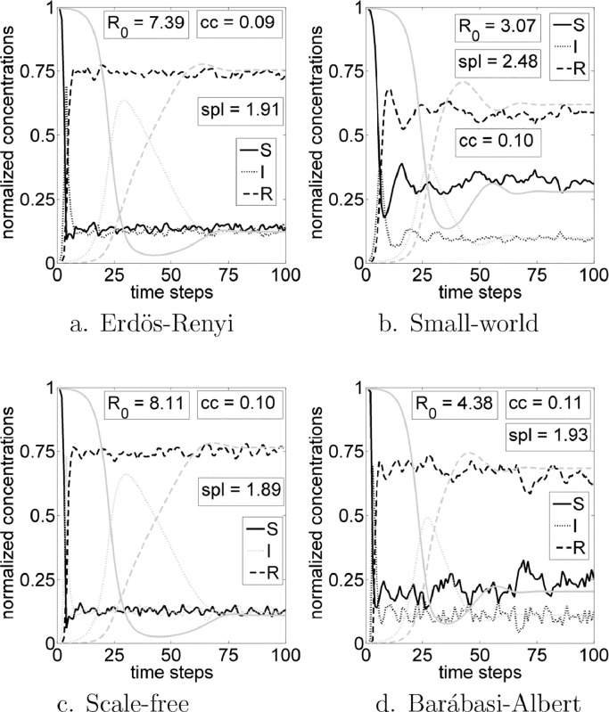
Fig. 1 exhibits the temporal evolutions for networks (a) Erdös–Rényi, (b) small-world, (c) Barbasi–Albert and (d) scale-free. Every R ₀ are indicated in the figure, as well the average clustering coefficient and average shortest path of each network. Light gray lines exhibit corresponding disease states for ODE simulations whose parameters where calculated from network simulations using Eq. (2). Note that the networks have similar topological parameters, however, R ₀ and the disease dynamic is different of each other. Furthermore, the temporal evolution of ODE and network models are different, though percentage of individuals in the steady state are similar. A good overview about the visual differences of how each network is created can be found at Shirley and Rushton (2005).

Fig. 1.

Network and ODE simulations with $k=0.1,$$P_c=60\%,$$P_d=30\%$ and $P_n=10\%$. For network simulations, susceptible state is represented by black solid line, infected is the black dotted line and recovered is the black dashed line. States of ODE simulations are in respective gray lines.

Therefore, here we simulate the disease spreading in a wide range of topological parameters for each complex network model. The tool for generating these networks is the C/C++ library iGraph (Csardi & Nepusz, 2006). The next sections formalize how the networks are stressed.

3.1. Erdös–Rényi

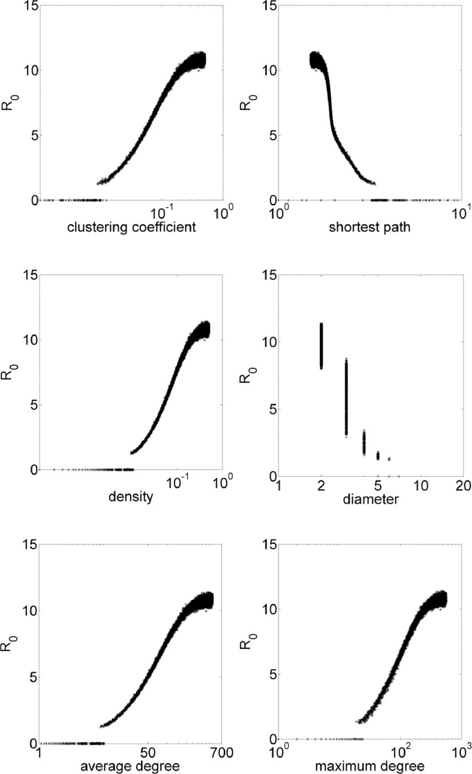
Considering a Erdös–Rényi network, a fraction p of all the possible edges is added to the network, that is, each possible edge has a probability of being added equal to p. The iGraph environment requires the value of p, thus, epidemiological model is simulated for each network with p in the range .0001:.0001:.5. In these simulations, average clustering coefficient results in values 0 ≲ cc ≲ 0.5, average shortest path, 1.5 ≲ spl ≲ 13, diameter, 2 ≲ diam ≲ 8, density, 0 ≲ den ≲ 0.5. Fig. 2 exhibits how these properties influences the value of R ₀. On Erdös–Rényi networks, cc ≈ p. See that in general, more connections mean higher values of R ₀. Distances measures indicate that with closer individuals (low shortest path and diameter), higher R ₀.

Fig. 2.

Erdös–Rényi simulations with R₀ in function of topological parameters clustering coefficient, shortest path, density, diameter, average degree and maximum degree.

3.2. Small-world

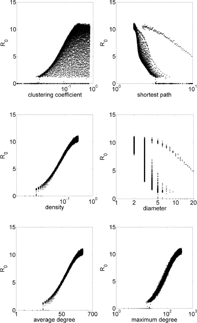
On small-world networks, each node starts with m connections with closer individuals. Then each connection is rewired with probability p, that is, any of the possible edges in the graph may be added by removing such connections. The iGraph environment requires the value of m and p, thus, epidemiological model is simulated for each network with p in the range .01:.01:1, and m in the range 1: 1: 150. In these simulations, average clustering coefficient results in values 0 ≲ cc ≲ 0.75, average shortest path, 1.78 ≲ spl ≲ 125, diameter, 2 ≲ diam ≲ 6, density, 0 ≲ den ≲ 0.2. Fig. 3 exhibits how these properties influences the value of R ₀.

Fig. 3.

Small-world simulations with R₀ in function of topological parameters clustering coefficient, shortest path, density, diameter, average degree and maximum degree.

Note that small-world networks are less dense than Erdös–Rényi networks with the same potential for a disease spreading depending on other topological features. Also, here, clustering coefficient is not enough to determine the value of R ₀, needing another parameter to verify disease spreading properties. The separated dots in shortest path and diameter figures are related to $p=0,$ when the network is regular with each node having the same number of connections m.

3.3. Scale-free

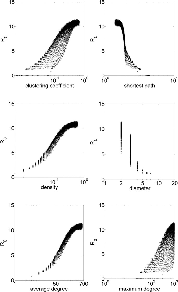
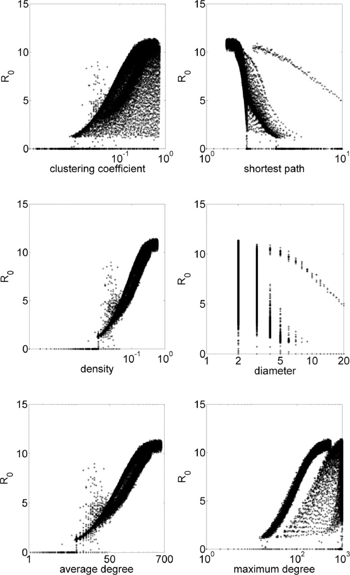
For scale-free networks, the number of edges e in the graph and the power law exponent γ determines the generation. That is, e edges are added to the network, and the probability that a node is chosen to get an edge is given by $P\left(k\right)=k^{\gamma },$ where k is the node degree. The iGraph environment requires the value of e and γ, thus, epidemiological model is simulated for each network with a fraction of possible edges q in the range 0.05:0.05:0.6, and γ in the range 2:0.1:6. In these simulations, average clustering coefficient results in values 0 ≲ cc ≲ 0.6, average shortest path, 1.4 ≲ spl ≲ 4.48, diameter, 2 ≲ diam ≲ 6, density, 0 ≲ den ≲ 0.6. Fig. 4 exhibits how these properties influences the value of R ₀.

Fig. 4.

Scale-free simulations with R₀ in function of topological parameters clustering coefficient, shortest path, density, diameter, average degree and maximum degree.

Scale-free network model allows a good range of topological parameters for the epidemiological model. Note that the model needs more edges in order to exhibit similar values of R ₀ than a small-world network, which is not so dense.

3.4. Barábasi–Albert

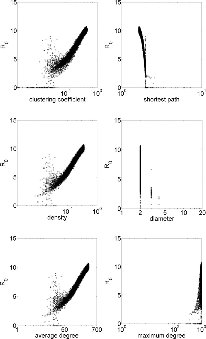
Barábasi–Albert network is a subset of scale-free networks. The difference is how the network is created, because Barábasi–Albert requires the exponent γ for the probability of a node being chosen to get an edge $P\left(k\right)=k^{\gamma },$ and the number of outgoing edges generated for each node m. The iGraph environment requires the value of m and γ, thus, epidemiological model is simulated for each network with m in the range 5: 5: 200, and γ in the range 2: 0.1: 5. In these simulations, average clustering coefficient results in values 0.01 ≲ cc ≲ 0.48, average shortest path, 1.67 ≲ spl ≲ 2.42, diameter, 2 ≲ diam ≲ 4, density, 0 ≲ den ≲ 0.36. Fig. 5 exhibits how these properties influences the value of R ₀.

Fig. 5.

Barábasi–Albert simulations with R₀ in function of topological parameters clustering coefficient, shortest path, density, diameter, average degree and maximum degree.

Such construction model generates networks with nodes with high degrees, and the consequence is the small range of the average shortest path. However, even for such small range, see that R ₀ abruptly fall from R ₀ ∼ 12 when average shortest path is spl ∼ 1.6, to R ₀ ∼ 2 when average shortest path is spl ∼ 2.4.

4. More results

In order to show the need of a more robust statistical analysis for all network data, all simulation results are show in Fig. 6 . Note that the average clustering coefficient, average shortest path, diameter and maximum degree is not enough to clearly identify a R ₀ prediction. Although there is a variance in data, density and average degree have trends which allow a R ₀ prediction. Moreover, R ₀ > 1, i.e., disease persists in population when den ≳ 0.01, and when average degree avdeg ≳ 10.

Fig. 6.

Data for all networks put together for R₀ in function of topological parameters clustering coefficient, shortest path, density, diameter, average degree and maximum degree.

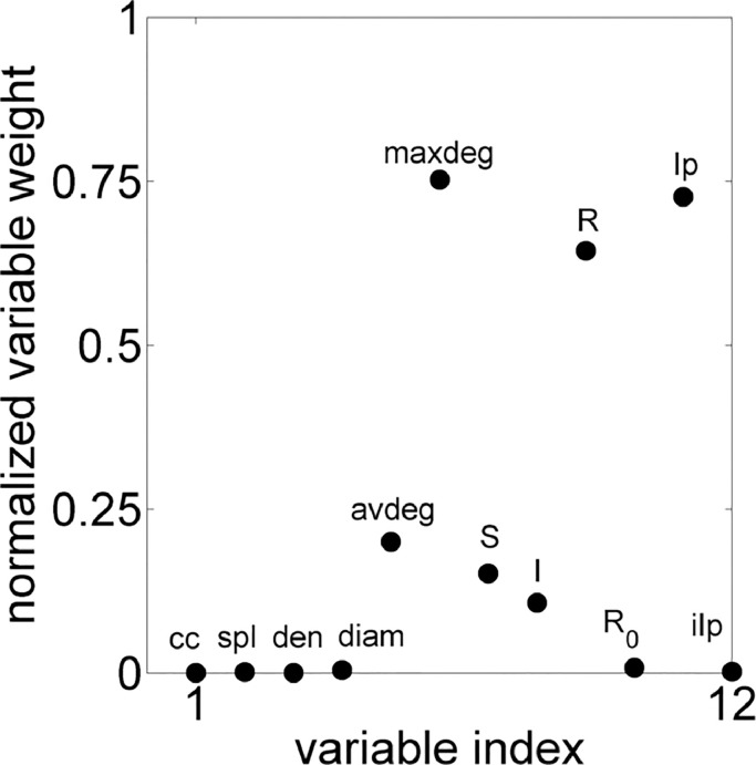
Therefore, PCA has been used to get other relationships between disease and network parameters. The variables used were: average clustering coefficient (cc); average shortest path (spl); density (den); diameter (diam); average degree (avdeg); maximum degree (maxdeg); amount of individuals Susceptible (S) Infected (I) and Recovered (R) when the system reached the permanent regime; Infected peak (Ip), (i.e., the amount of Infected individuals in the initial outbreak of disease) and; instant of Infected peak (iIp), which is the time step when the peak occurred. All these 12 variables have been considered for all 41,270 experiments of all networks and the Fig. 7 contains the normalized projection of each variable.

Fig. 7.

PCA results infographic.

Note that according to PCA, the internal structure of the data that best explains the variance in the data have maxdeg, Ip, R and avdeg as most informative variables. Fig 6 already exhibited R ₀ in function of maxdeg, and such variable certainly does not explain the disease variables. Actually, the maximum degree of the network is very sensitive to the other topological parameters for all networks.

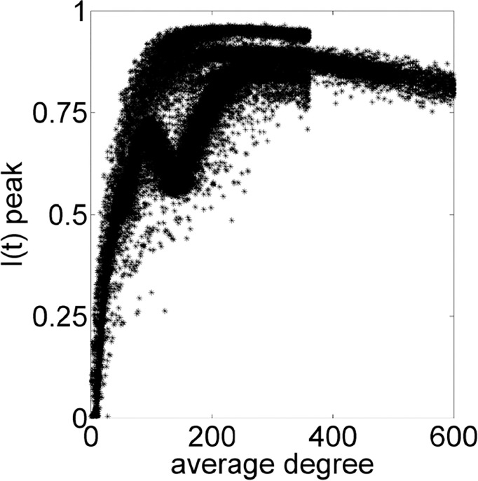
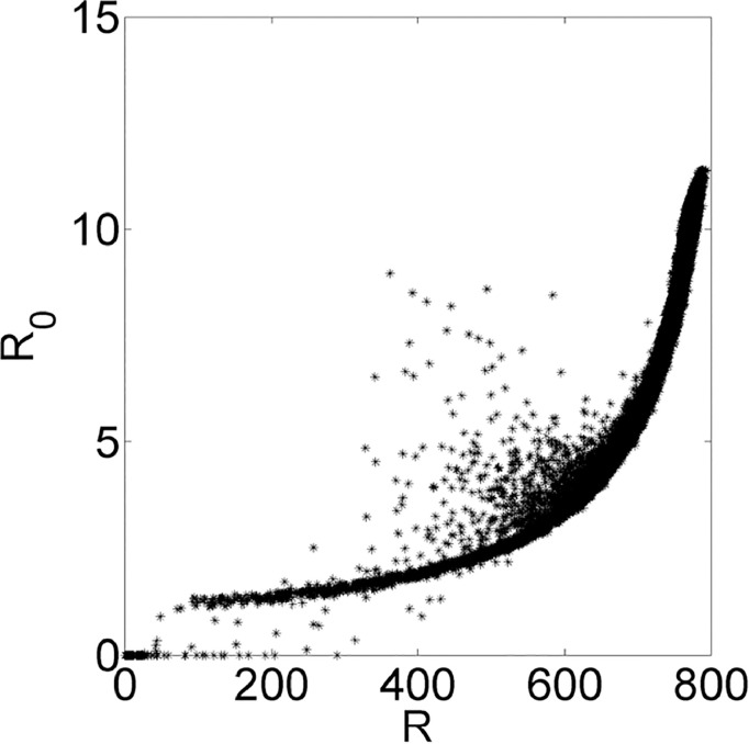
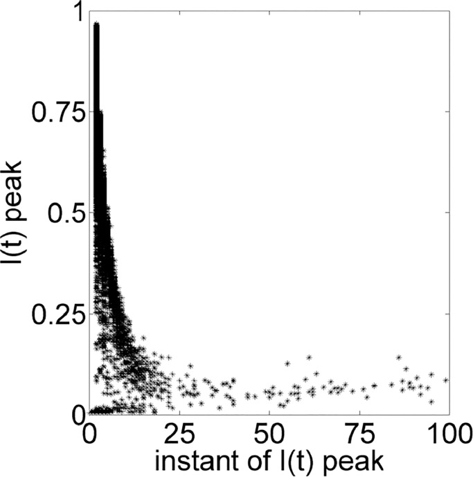
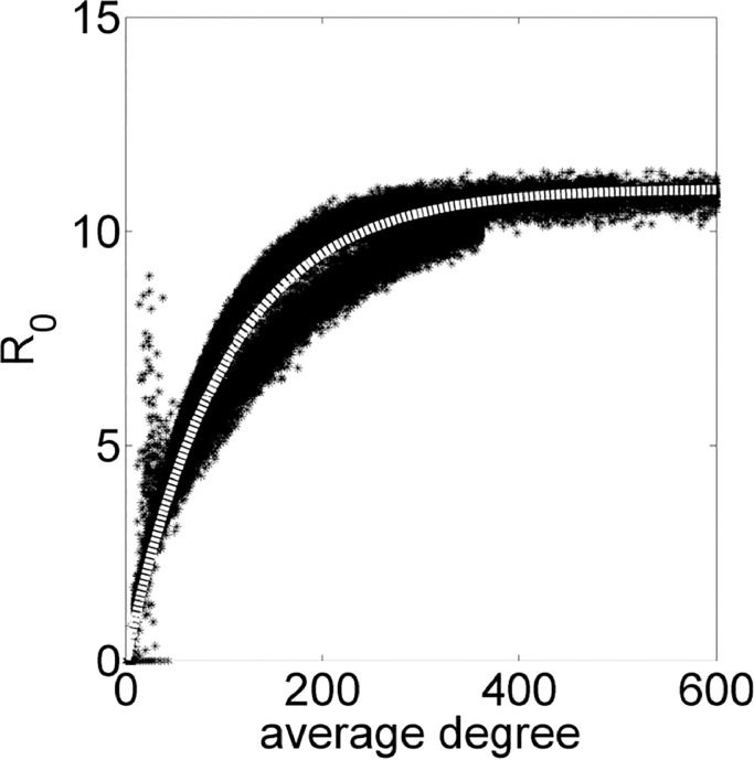
Thereby, relationships on Figs. 8 –11 are based on PCA results. The Fig. 8 shows that small values of average degree is enough for a high peak of infected individuals and the trend of increasing the I(t) peak changes at around 300, when it starts to decrease. Fig. 9 indicates that the sooner the I(t) occurs, the high the value of the peak is. Fig. 10 contains the same data of Fig. 6 for average degree, but in a different scale. Somehow, PCA confirms the importance of the average degree for analyzing a disease spreading.

Fig. 8.

Peak instant of I(t) in function of average degree of the network.

Fig. 11.

R₀ in function of the average recovered individuals R when system reached its permanent regime.

Fig. 9.

Peak instant of I(t) in function of I(t) peak.

Fig. 10.

R₀ in function of the network average degree.

Note that for all figures, the value of R ₀ saturates. In such condition, the term aS(t)I(t) of Eq. (1) can be written as $aS\left(t\right)I\left(t\right)=S\left(t\right),$ since all Susceptible individuals become infected. Accordingly, the new equations are:

$$\begin{array}{ccc}\hfill \frac{dS\left(t\right)}{dt}& =& -S\left(t\right)+cI\left(t\right)+eR\left(t\right)\hfill \\ \hfill \frac{dI\left(t\right)}{dt}& =& S\left(t\right)-bI\left(t\right)-cI\left(t\right)\hfill \\ \hfill \frac{dR\left(t\right)}{dt}& =& bI\left(t\right)-eR\left(t\right)\hfill \end{array}$$ (3)

with the set of stationary solutions (as done for Eq. (1)): $(S_{sat}^{*},I_{sat}^{*},R_{sat}^{*})=(1,0,0)$ and $(S_{sat}^{*},I_{sat}^{*},R_{sat}^{*})=(e(b+c)/(b+e(b+c+1)),e/(b+e(b+c+1)),b/(b+e(b+c+1)))$. Therefore, we have $a_{sat}=1/I_{sat}^{*},$ thus:

$$\begin{array}{c}\hfill R_{0sat}=\frac{a_{sat}}{b+c}=\frac{1/I_{sat}^{*}}{b+c}=\frac{b+e(b+c+1)}{e(b+c)}\end{array}$$ (4)

Using Eq. (2) for determining values for b, c and e, we have $R_{0sat}=11$. Thus, the white thick dashed line in Fig. 10 is a fitted curve for the experimental points in the form:

$$R_0\left(avdeg\right)=R_{0sat}*(1-e^{-\alpha *avdeg})$$

where $\alpha =0.0099$.

Finally, a distinct result is presented on Fig. 11, where the R ₀ is plotted in function of the amount of Recovered individuals (R) when the system reached the permanent regime. Here, the disease R ₀ increases when R increases and this result is corroborated by other related papers, since the disease qualitatively parameters used are usually from diseases like mumps, chickenpox and measles (Monteiro, Chimara, & Berlinck, 2006) which also have high R ₀ and high amount of Recovered individuals in population (Anderson & May, 1991). If we consider that the permanent regime of the system has R ₀ > 1, i.e., disease is active, R ₀ can be approximated by $R_0=b/(b-R^{*}(e+b))$.

5. Discussion

In this paper, we presented a method to understand a disease propagation according to the most important topological parameters of four types of complex networks. Disease were modeled by SIR-model, population by networks Erdös–Rényi, Small-World, Scale-Free and Barábasi–Albert and the statistical process to analyze the data were Principal Component Analysis. Based on the results, following characteristics of epidemic outbreaks in populations emerged as most important factors: average degree, infected individuals peak, instant that such peak occurs, amount of recovered individuals in system steady-state and, of course, the basic reproduction number, R ₀.

Topological parameters like clustering coefficient and shortest path length, which are often used to analyze disease spreading on networks (Dorjee, Revie, Poljak, McNab, Sanchez, 2013, Keeling, 2005, Lennartsson, Håkansson, Wennergren, Jonsson, 2012, Moslonka-Lefebvre, Pautasso, Jeger, 2009, Oleś, Gudowska-Nowak, Kleczkowski, 2014, Raymond, Hosie, 2009, Schimit, Monteiro, 2009), should not be used when many network models are considered or the model is unknown, though they are robust when the model is well defined. Therefore, considering that social networks may not be properly represented by a determined model, as well as assumptions for modeling may not be correct, a careful parameter choice for analyzing disease propagation must be done, as concluded in Shirley and Rushton (2005). Here, we presented some parameter to consider, like the average degree, density and the amount of Recovered individuals. Moreover, results came from a wide range of networks: from highly concentrated connections, like Barábasi–Albert networks, to Erdös–Rényi model, where connections are equally distributed over the population. Nevertheless, average degree were an important topological parameter, also noted in Colizza et al. (2007).

Lastly, the simulation diversity made it possible to verify a saturation in R ₀ value, that is, a maximum value for R ₀ given the epidemiological parameters, like the probability of recovering from disease, probability of dying due to disease and probability for dying from natural causes. Such saturation occurs when all Susceptible individuals get infected at each time-step. High value of R ₀, most part of population in Recovered state, almost all Susceptible individuals getting infected are characteristics of a well known scenario for child diseases like mumps, chickenpox and measles if a age stratified population is considered (Wallinga, Teunis, & Kretzschmar, 2006).

Considering the possibilities of future work directions, they should handle with following questions:

• •Is the PCA approach used here suitable to other diseases models as well as populations modeled by another multi-agent environment, like cellular automata (Holko et al., 2016)?
• •Is the PCA approach suitable to other uses of populations, like evolutionary algorithms (Bajer, Martinovi, Brest, 2016, Chang, Chen, Lin, 2005, Li, Zhang, Zeng, 2009) and general population dynamics (Simidjievski et al., 2015)?
• •Considering mathematical epidemiology, the inclusion of methods to control the spread of the disease to the model could return the most effective to combat the disease. Vaccination and limiting contacts between individuals should be tested;
• •The calculation of R ₀ is usually difficult in the first cases of a disease outbreak (Mossong & Muller, 2000). The PCA model could be used in the initial transient of disease with partial information to return the most important variables to consider to approximate the R ₀ value.

References

- Aladeemy M., Tutun S., Khasawneh M.T. A new hybrid approach for feature selection and support vector machine model selection based on self-adaptive cohort intelligence. Expert Systems with Applications. 2017;88:118–131. [Google Scholar]
- Albert R., Barabasi A.L. Statistical mechanics of complex networks. Reviews of Modern Physics. 2002;74(1):47–97. [Google Scholar]
- Anderson R.M., May R.M. Oxford University Press; Oxford, New York: 1991. Infectious diseases of humans: Dynamics and control. (Oxford science publications). [Google Scholar]
- Bajer D., Martinovi G., Brest J. A population initialization method for evolutionary algorithms based on clustering and cauchy deviates. Expert Systems with Applications. 2016;60(Suppl C):294–310. [Google Scholar]
- Balcan D., Gonçalves B., Hu H., Ramasco J.J., Colizza V., Vespignani A. Modeling the spatial spread of infectious diseases: The global epidemic and mobility computational model. Journal of Computational Science. 2010;1(3):132–145. doi: 10.1016/j.jocs.2010.07.002. [DOI] [PMC free article] [PubMed] [Google Scholar]
- Bansal S., Meyers L.A. The impact of past epidemics on future disease dynamics. Journal of Theoretical Biology. 2012;309:176–184. doi: 10.1016/j.jtbi.2012.06.012. [DOI] [PubMed] [Google Scholar]
- Barabási A.-L., Albert R. Emergence of scaling in random networks. Science. 1999;286(5439):509–512. doi: 10.1126/science.286.5439.509. [DOI] [PubMed] [Google Scholar]
- Bigras-Poulin M., Thompson R.A., Chriel M., Mortensen S., Greiner M. Network analysis of danish cattle industry trade patterns as an evaluation of risk potential for disease spread. Preventive Veterinary Medicine. 2006;76(1–2):11–39. doi: 10.1016/j.prevetmed.2006.04.004. [DOI] [PubMed] [Google Scholar]
- Boccaletti S., Latora V., Moreno Y., Chavez M., Hwang D.U. Complex networks: Structure and dynamics. Physics Reports. 2006;424(4–5):175–308. [Google Scholar]
- Bollobás B., Riordan O., Spencer J., Tusndy G. The degree sequence of a scale-free random graph process. Random Structures & Algorithms. 2001;18(3):279–290. [Google Scholar]
- Chang P.-C., Chen S.-H., Lin K.-L. Two-phase sub population genetic algorithm for parallel machine-scheduling problem. Expert Systems with Applications. 2005;29(3):705–712. [Google Scholar]
- Colizza V., Barthélemy M., Barrat A., Vespignani A. Epidemic modeling in complex realities. Comptes Rendus – Biologies. 2007;330(4):364–374. doi: 10.1016/j.crvi.2007.02.014. [DOI] [PubMed] [Google Scholar]
- Colizza V., Vespignani A. Epidemic modeling in metapopulation systems with heterogeneous coupling pattern: Theory and simulations. Journal of Theoretical Biology. 2008;251(3):450–467. doi: 10.1016/j.jtbi.2007.11.028. [DOI] [PubMed] [Google Scholar]
- Csardi G., Nepusz T. The iGraph software package for complex network research. InterJournal, Complex Systems. 2006;1695:1–9. [Google Scholar]
- Dorjee S., Revie C.W., Poljak Z., McNab W.B., Sanchez J. Network analysis of swine shipments in Ontario, Canada, to support disease spread modelling and risk-based disease management. Preventive Veterinary Medicine. 2013;112(1–2):118–127. doi: 10.1016/j.prevetmed.2013.06.008. [DOI] [PubMed] [Google Scholar]
- Elangovan M., Devasenapati S.B., Sakthivel N.R., Ramachandran K.I. Evaluation of expert system for condition monitoring of a single point cutting tool using principle component analysis and decision tree algorithm. Expert Systems with Applications. 2011;38(4):4450–4459. [Google Scholar]
- Erdos P., Rényi A. On random graphs, I. Publicationes Mathematicae. 1959;6:290–297. [Google Scholar]
- Franc A. Metapopulation dynamics as a contact process on a graph. Ecological Complexity. 2004;1(1):49–63. [Google Scholar]
- Guo Q., Wu W., Massart D.L., Boucon C., Jong S.D. Feature selection in principal component analysis of analytical data. Chemometrics and Intelligent Laboratory Systems. 2002;61:123–132. [Google Scholar]
- Guyon I. An introduction to variable and feature selection. Journal of Machine Learning Research. 2003;3:1157–1182. [Google Scholar]
- Holko A., Mdrek M., Pastuszak Z., Phusavat K. Epidemiological modeling with a population density map-based cellular automata simulation system. Expert Systems with Applications. 2016;48:1–8. [Google Scholar]
- Jeger M.J., Pautasso M., Holdenrieder O., Shaw M.W. Modelling disease spread and control in networks: implications for plant sciences. The New Phytologist. 2007;174(2):279–297. doi: 10.1111/j.1469-8137.2007.02028.x. [DOI] [PubMed] [Google Scholar]
- Jolliffe I. (2nd ed.) Springer; 2002. Principal component analysis. [Google Scholar]
- Keeling M. The implications of network structure for epidemic dynamics. Theoretical Population Biology. 2005;67(1):1–8. doi: 10.1016/j.tpb.2004.08.002. [DOI] [PubMed] [Google Scholar]
- Keeling M., Rand D., Morris A. Correlation models for childhood epidemics. Proceedings of the Royal Society B: Biological Sciences. 1997;264(1385):1149–1156. doi: 10.1098/rspb.1997.0159. [DOI] [PMC free article] [PubMed] [Google Scholar]
- Kermack W.O., McKendrick A.G. A contribution to the mathematical theory of epidemics. Proceedings of the Royal Society of London A: Mathematical, Physical and Engineering Sciences. 1927;115(772):700–721. [Google Scholar]
- Legara E.F.T., Monterola C.P., David C. Complex network tools in building expert systems that perform framing analysis. Expert Systems with Applications. 2013;40(11):4600–4608. [Google Scholar]
- Lennartsson J., Håkansson N., Wennergren U., Jonsson A. SpecNet: A spatial network algorithm that generates a wide range of specific structures. PloS One. 2012;7(8):e42679. doi: 10.1371/journal.pone.0042679. [DOI] [PMC free article] [PubMed] [Google Scholar]
- Li Y., Zhang S., Zeng X. Research of multi-population agent genetic algorithm for feature selection. Expert Systems with Applications. 2009;36(9):11570–11581. [Google Scholar]
- Lu Y., Cohen I., Zhou X.S., Tian Q. Proceedings of the fifteenth ACM international conference on multimedia, MM ’07. ACM; New York, NY, USA: 2007. Feature selection using principal feature analysis; pp. 301–304. [Google Scholar]
- May R.M. Network structure and the biology of populations. Trends in Ecology and Evolution. 2006;21(7):394–399. doi: 10.1016/j.tree.2006.03.013. [DOI] [PubMed] [Google Scholar]
- Monteiro L., Chimara H., Berlinck J. Big cities: Shelters for contagious diseases. Ecological Modelling. 2006;197:258–262. [Google Scholar]
- Monteiro L., Sasso J., Berlinck J.C. Continuous and discrete approaches to the epidemiology of viral spreading in populations taking into account the delay of incubation time. Ecological Modelling. 2007;201(34):553–557. [Google Scholar]
- Moore C., Newman M.E.J. Epidemics and percolation in small-world networks. Physical Review E. 2000;61(5):5678–5682. doi: 10.1103/physreve.61.5678. [DOI] [PubMed] [Google Scholar]
- Moreno Y., Pastor-Satorras R., Vespignani A. Epidemic outbreaks in complex heterogeneous networks. The European Physical Journal B – Condensed Matter and Complex Systems. 2002;26(4):521–529. [Google Scholar]
- Moslonka-Lefebvre M., Harwood T., Jeger M.J., Pautasso M. SIS along a continuum (SIS(c)) epidemiological modelling and control of diseases on directed trade networks. Mathematical Biosciences. 2012;236(1):44–52. doi: 10.1016/j.mbs.2012.01.004. [DOI] [PubMed] [Google Scholar]
- Moslonka-Lefebvre M., Pautasso M., Jeger M.J. Disease spread in small-size directed networks: Epidemic threshold, correlation between links to and from nodes, and clustering. Journal of Theoretical Biology. 2009;260(3):402–411. doi: 10.1016/j.jtbi.2009.06.015. [DOI] [PubMed] [Google Scholar]
- Mossong J., Muller C.P. Estimation of the basic reproduction number of measles during an outbreak in a partially vaccinated population. Epidemiology and Infection. 2000;1(124):273–278. doi: 10.1017/s0950268899003672. [DOI] [PMC free article] [PubMed] [Google Scholar]
- Newman M. Oxford University Press, Inc; New York, NY, USA: 2010. Networks: An introduction. [Google Scholar]
- Oleś K., Gudowska-Nowak E., Kleczkowski A. Understanding disease control: Influence of epidemiological and economic factors. PloS One. 2012;7(5):e36026. doi: 10.1371/journal.pone.0036026. [DOI] [PMC free article] [PubMed] [Google Scholar]
- Oleś K., Gudowska-Nowak E., Kleczkowski A. Cost-benefit analysis of epidemics spreading on clustered random networks. Acta Physica Polonica B. 2014;45(1):43. [Google Scholar]
- Óskarsdóttir M., Bravo C., Verbeke W., Sarraute C., Baesens B., Vanthienen J. Social network analytics for churn prediction in Telco: Model building, evaluation and network architecture. Expert Systems with Applications. 2017;85:204–220. [Google Scholar]
- Pellis L., Ferguson N.M., Fraser C. Threshold parameters for a model of epidemic spread among households and workplaces. Journal of the Royal Society Interface. 2009;6(February):979–987. doi: 10.1098/rsif.2008.0493. [DOI] [PMC free article] [PubMed] [Google Scholar]
- Rautureau S., Dufour B., Durand B. Vulnerability of animal trade networks to the spread of infectious diseases: A methodological approach applied to evaluation and emergency control strategies in cattle, France, 2005. Transboundary and Emerging Diseases. 2010;58:110–120. doi: 10.1111/j.1865-1682.2010.01187.x. [DOI] [PubMed] [Google Scholar]
- van Ravensway J., Benbow M.E., Tsonis A.A., Pierce S.J., Campbell L.P., Fyfe J.a.M. Climate and landscape factors associated with Buruli ulcer incidence in Victoria, Australia. PloS One. 2012;7(12):e51074. doi: 10.1371/journal.pone.0051074. [DOI] [PMC free article] [PubMed] [Google Scholar]
- Raymond B., Hosie G. Network-based exploration and visualisation of ecological data. Ecological Modelling. 2009;220(5):673–683. [Google Scholar]
- Riley S. Models of infectious disease. Science. 2007;316(5829):1298–1301. doi: 10.1126/science.1134695. [DOI] [PubMed] [Google Scholar]
- Roy M., Pascual M. On representing network heterogeneities in the incidence rate of simple epidemic models. Ecological Complexity. 2006;3(1):80–90. [Google Scholar]
- Sander L.M., Warren C.P., Sokolov I., Simon C., Koopman J. Percolation on disordered networks as a model for epidemics. Mathematical Biosciences. 2002;180:293–305. doi: 10.1016/s0025-5564(02)00117-7. [DOI] [PubMed] [Google Scholar]
- Schimit P., Monteiro L. On the basic reproduction number and the topological properties of the contact network: An epidemiological study in mainly locally connected cellular automata. Ecological Modelling. 2009;220:1034–1042. doi: 10.1016/j.ecolmodel.2009.01.014. [DOI] [PMC free article] [PubMed] [Google Scholar]
- Shirley M.D.F., Rushton S.P. The impacts of network topology on disease spread. Ecological Complexity. 2005;2(3):287–299. [Google Scholar]
- Simidjievski N., Todorovski L., Deroski S. Predicting long-term population dynamics with bagging and boosting of process-based models. Expert Systems with Applications. 2015;42(22):8484–8496. [Google Scholar]
- Tao Z., Zhongqian F., Binghong W. Epidemic dynamics on complex networks. Progress in Natural Science. 2006;16(5):452–457. [Google Scholar]
- Tildesley M.J., House T.a., Bruhn M.C., Curry R.J., O’Neil M., Allpress J.L.E. Impact of spatial clustering on disease transmission and optimal control. Proceedings of the National Academy of Sciences of the United States of America. 2010;107(3):1041–1046. doi: 10.1073/pnas.0909047107. [DOI] [PMC free article] [PubMed] [Google Scholar]
- Trapman P. On analytical approaches to epidemics on networks. Theoretical Population Biology. 2007;71:160–173. doi: 10.1016/j.tpb.2006.11.002. [DOI] [PubMed] [Google Scholar]
- Vazquez-Prokopec G.M., Kitron U., Montgomery B., Horne P., Ritchie S.A. Quantifying the spatial dimension of dengue virus epidemic spread within a tropical urban environment. PLoS Neglected Tropical Diseases. 2010;4(12):1–14. doi: 10.1371/journal.pntd.0000920. [DOI] [PMC free article] [PubMed] [Google Scholar]
- Verdasca J., Telo da Gama M.M., Nunes A., Bernardino N.R., Pacheco J.M., Gomes M.C. Recurrent epidemics in small world networks. Journal of Theoretical Biology. 2005;233(4):553–561. doi: 10.1016/j.jtbi.2004.10.031. [DOI] [PubMed] [Google Scholar]
- Wachs-Lopes G.A., Rodrigues P.S. Analyzing natural human language from the point of view of dynamic of a complex network. Expert Systems with Applications. 2016;45:8–22. [Google Scholar]
- Wallinga J., Teunis P., Kretzschmar M. Original contribution using data on social contacts to estimate age-specific transmission parameters for respiratory-spread infectious agents. American Journal of Epidemiology. 2006;164(10):936–944. doi: 10.1093/aje/kwj317. [DOI] [PubMed] [Google Scholar]
- Wang L., Li X., Zhang Y.Q., Zhang Y., Zhang K. Evolution of scaling emergence in large-scale spatial epidemic spreading. PLoS One. 2011;6(7):1–11. doi: 10.1371/journal.pone.0021197. [DOI] [PMC free article] [PubMed] [Google Scholar]
- Watts D., Strogatz S. Collective dynamics of small-world networks. Nature. 1998;393:440–442. doi: 10.1038/30918. [DOI] [PubMed] [Google Scholar]
- Westgarth C., Gaskell R.M., Pinchbeck G.L., Bradshaw J.W.S., Dawson S., Christley R.M. Walking the dog: Exploration of the contact networks between dogs in a community. Epidemiology and Infection. 2009;137(8):1169–1178. doi: 10.1017/S0950268808001544. [DOI] [PubMed] [Google Scholar]
- Xiao Y., Zhou Y., Tang S. Modelling disease spread in dispersal networks at two levels. Mathematical Medicine and Biology: A Journal of the IMA. 2011;28(3):227–244. doi: 10.1093/imammb/dqq007. [DOI] [PubMed] [Google Scholar]
- Zhong S., Huang Q., Song D. Simulation of the spread of infectious diseases in a geographical environment. Science in China Series D: Earth Sciences. 2009;52(4):550–561. doi: 10.1007/s11430-009-0044-9. [DOI] [PMC free article] [PubMed] [Google Scholar]