APPLES: Scalable Distance-Based Phylogenetic Placement with or without Alignments

Abstract

Placing a new species on an existing phylogeny has increasing relevance to several applications. Placement can be used to update phylogenies in a scalable fashion and can help identify unknown query samples using (meta-)barcoding, skimming, or metagenomic data. Maximum likelihood (ML) methods of phylogenetic placement exist, but these methods are not scalable to reference trees with many thousands of leaves, limiting their ability to enjoy benefits of dense taxon sampling in modern reference libraries. They also rely on assembled sequences for the reference set and aligned sequences for the query. Thus, ML methods cannot analyze data sets where the reference consists of unassembled reads, a scenario relevant to emerging applications of genome skimming for sample identification. We introduce APPLES, a distance-based method for phylogenetic placement. Compared to ML, APPLES is an order of magnitude faster and more memory efficient, and unlike ML, it is able to place on large backbone trees (tested for up to 200,000 leaves). We show that using dense references improves accuracy substantially so that APPLES on dense trees is more accurate than ML on sparser trees, where it can run. Finally, APPLES can accurately identify samples without assembled reference or aligned queries using kmer-based distances, a scenario that ML cannot handle. APPLES is available publically at github.com/balabanmetin/apples.

Phylogenetic placement is the problem of finding the optimal position for a new query species on an existing backbone (or, reference) tree. Placement, as opposed to a de novo reconstruction of the full phylogeny, has two advantages. In some applications (discussed below), placement is all that is needed, and in terms of accuracy, it is as good as, and even better than (Janssen et al. 2018), de novo reconstruction. Moreover, placement can be more scalable than de novo reconstruction when dealing with very large trees.

Earlier research on placement was motivated by scalability. For example, placement is used in greedy algorithms that start with an empty tree and add sequences sequentially (e.g., Felsenstein 1981; Desper and Gascuel 2002). Each placement requires polynomial (often linear) time with respect to the size of the backbone, and thus, these greedy algorithms are scalable (often requiring quadratic time). Despite computational challenges (Warnow 2017), there has been much progress in the de novo reconstruction of ultralarge trees (e.g., thousands to millions of sequences) using both maximum likelihood (ML) (e.g., Price et al. 2010; Nguyen et al. 2015) and the distance-based (e.g., Lefort et al. 2015) approaches. However, these large-scale reconstructions require significant resources. As new sequences continually become available, placement can be used to update existing trees without repeating previous computations on full data set.

More recently, placement has found a new application in sample identification: given one or more query sequences of unknown origins, detect the identity of the (set of) organism(s) that could have generated that sequence. These identifications can be made easily using sequence matching tools such as BLAST (Altschul et al. 1990) when the query either exactly matches or is very close to a sequence in the reference library. However, when the sequence is novel (i.e., has lowered similarity to known sequences in the reference), this closest match approach is not sufficiently accurate (Koski and Golding 2001), leading some researchers to adopt a phylogenetic approach (Sunagawa et al. 2013; Nguyen et al. 2014). Sample identification is essential to the study of mixed environmental samples, especially of the microbiome, both using 16S profiling (e.g., Gill et al. 2006; Krause et al. 2008) and metagenomics (e.g., von Mering et al. 2007). It is also relevant to barcoding (Hebert et al. 2003) and metabarcoding (Clarke et al. 2014; Bush et al. 2017) and quantification of biodiversity (e.g., Findley et al. 2013). Driven by applications to microbiome profiling, placement tools like pplacer (Matsen et al. 2010) and evolutionary placement algorithm (EPA(-ng)) (Berger et al. 2011; Barbera et al. 2019) have been developed. Researchers have also developed methods for aligning query sequence (e.g., Berger and Stamatakis 2011; Mirarab et al. 2012) and for downstream steps (e.g., Stark et al. 2010; Matsen and Evans 2013). These publications have made a strong case that for sample identification, placement is sufficient (i.e., de novo is not needed). Moreover, some studies (e.g., Janssen et al. 2018) have shown that when dealing with fragmentary reads typically found in microbiome samples, placement can be more accurate than de novo construction and can lead to improved associations of microbiome with clinical information.

Existing phylogenetic placement methods have focused on the ML inference of the best placement—a successful approach, which nevertheless, suffers from two shortcomings. On the one hand, ML can only be applied when the reference species are assembled into full-length sequences (e.g., an entire gene) and are aligned; however, in new applications that we will describe, assembling (and hence aligning) the reference set is not possible. On the other hand, ML, while somewhat scalable, is still computationally demanding, especially in memory usage, and cannot place on backbone trees with many thousands of leaves. As the density of reference substantially impacts the accuracy and resolution of placement, this inability to use ultralarge trees as backbone also limits accuracy. This limitation has motivated alternative methods using local sensitive hashing (Brown and Truszkowski 2013) and divide-and-conquer (Mirarab et al. 2012).

Assembly-free and alignment-free sample identification using genome skimming (Dodsworth 2015) can also benefit from phylogenetic placement. A genome skim is a shotgun sample of the genome sequenced at low coverage (e.g., 1X)—so low that assembling the nuclear genome is not possible (though, mitochondrial or plastid genomes can often be assembled). Genome skimming promises to replace traditional marker-based barcoding of biological samples (Coissac et al. 2016) but limiting analyses to organelle genome can limit resolution. Moreover, mapping reads to reference genomes is also possible only for species that have been assembled, which is a small fraction of the biodiversity on Earth. Sarmashghi et al. (2019) have recently shown that using shared -mers, the distance between two unassembled genome skims with low coverage can be accurately estimated. This approach, unlike assembling organelle genomes, uses data from the entire nuclear genome and hence promises to provide a higher resolution (e.g., at species or subspecies levels) while keeping the low sequencing cost. However, ML and other methods that require assembled sequences cannot analyze genome skims, where both the reference and the query species are unassembled genome-wide bags of reads.

Distance-based approaches to phylogenetics are well-studied, but no existing tool can perform distance-based placement of a query sequence on a given backbone. The distance-based approach promises to solve both shortcomings of ML methods. Distance-based methods are computationally efficient and do not require assemblies. They only need distances (however computed). Thus, they can take as input assembly-free estimates of genomic distance estimated from low coverage genome skims using Skmer (Sarmashghi et al. 2019) or other alternatives (Yi and Jin 2013; Haubold 2014; Fan et al. 2015; Benoit et al. 2016; Ondov et al. 2016; Leimeister et al. 2017; Jain et al. 2018). While alignment-based phylogenetics has been traditionally more accurate than alignment-free methods when both methods are possible, in these new scenarios, only alignment-free methods are applicable.

Here, we introduce a new method for distance-based phylogenetic placement called APPLES (Accurate Phylogenetic Placement using LEast Squares). APPLES uses dynamic programming to find the optimal distance-based placement of a sequence with running time and memory usage that scale linearly with the size of the backbone tree. We test APPLES in simulations and on real data, both for alignment-free and aligned scenarios.

Description

Background and Notations

Let an unrooted tree be a weighted connected acyclic undirected graph with leaves denoted by . We let be the rooting of on a leaf obtained by directing all edges away from . For node , let denote its parent, denote its set of children, denote its siblings, and denote the set of leaves at or below (i.e., those that have on their path to the root), all with respect to . Also let denote the length of the edge .

The tree defines an matrix where each entry corresponds to the path length between leaves and . We further generalize this definition so that indicates the length of the undirected path between any two nodes of (when clear, we simply write ). Given some input data, we can compute a matrix of all pairwise sequence distances , where the entry indicates the dissimilarity between species and . When the sequence distance is computed using (the correct) phylogenetic model, it will be a noisy but statistically consistent estimate of the tree distance (Felsenstein 2003). Given these “phylogenetically corrected” distances (e.g. is the corrected hamming distance under the Jukes and Cantor (1969) model), we can define optimization problems to recover the tree that best fits the distances. A natural choice is minimizing the (weighted) least square difference between tree and sequence distances:

(1)

Here, weights (e.g., ) are used to reduce the impact of large distances (expected to have high variance). A general weighting schema can be defined as for a constant value . Standard choices of include for the ordinary least squares (OLS) method of Cavalli-Sforza and Edwards 1967, due to Beyer et al. 1974 (BE), and due to Fitch and Margoliash 1967 (FM).

Finding is NP-Complete (Day and Sankoff 1987). However, decades of research has produced heuristics like neighbor-joining (Saitou and Nei 1987), alternative formulations like (balanced) minimum evolution (ME) (Cavalli-Sforza and Edwards 1967; Desper and Gascuel 2002), and several effective tools for solving the problem heuristically (e.g., FastME by Lefort et al. 2015, DAMBE by Xia 2018, and Ninja by Wheeler 2009).

Problem Statement

We let be the tree obtained by adding a query taxon on an edge , creating three edges , , and , with lengths , , and , respectively (Fig. 1). When clear, we simply write and note that induces both in topology and branch length. We now define the problem.

Figure 1.

Any placement of can be characterized as a tree , shown here. The backbone tree is an arborescence on leaves , rooted at leaf . Query taxon is added on the edge between and , creating a node . All placements on this edge are characterized by , the length of the pendant branch, and , the distance between and .

• Least squares phylogenetic placement (LSPP):

  • [Input:] A backbone tree on , a query species , and a vector with elements giving sequence distances between and every species ;

  • [Output:] The placement tree that adds on and minimizes

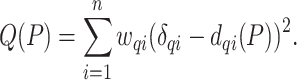
    (2)

Linear Time Algorithm

The number of possible placements of is . Therefore, LSPP can be solved by simply iterating over all the topologies, optimizing the score for that branch, and returning the placement with the minimum least square error. A naive algorithm can accomplish this in running time by optimizing Eq. 2 for each of the branches. However, using dynamic programming, the optimal solution can be found in linear time.

Theorem 1.

The LSPP problem can be solved with running time and memory.

The proof (given in Supplementary Appendix 1 available on Dryad at https://doi.org/10.5061/dryad.78nf7dq) follows easily from three lemmas that we next state. The algorithm starts with precomputing a fixed-size set of values for each nodes. For any node and exponents and , let and for , let . Note that . Similarly, for , let for and let .

Lemma 2.

The set of all and values can be precomputed in time with two tree traversals using the dynamic programming given by:

(3)

(4)

Lemma 3.

Equation 2 can be rearranged (see Supplementary Appendix 1, Eq. S2 available on Dryad) such that computing for a given requires a constant time computation using and values for and .

Thus, after a linear time precomputation, we can compute the error for any given placement in constant time. It remains to show that for each node, the optimal placement on the branch above it (e.g., and ) can be computed in constant time.

Lemma 4.

For a fixed node , if , then

(5)

and hence can be computed in constant time.

Non-negative branch lengths

The solution to Equation 5 does not necessarily conform to constraints and . However, the following lemma (proof in Supplementary Appendix 1 available on Dryad) allows us to easily impose the constraints by choosing optimal boundary points when unrestricted solutions fall outside boundaries.

Lemma 5.

With respect to variables and , is a convex function.

Minimum evolution

An alternative to directly using minimum least square error (MLSE) (Eq. 1) is the ME principle (Cavalli-Sforza and Edwards 1967; Rzhetsky and Nei 1992). Our algorithm can also optimize the ME criterion: after computing and by optimizing MLSE for each node , we choose the placement with the minimum total branch length. This is equivalent to using , since the value of does not contribute to total branch length. Other solutions for ME placement exist (Desper and Gascuel 2002), a topic we return to in the Discussion section.

Hybrid

We have observed cases where ME is correct more often than MLSE, but when it is wrong, unlike MLSE, it has a relatively high error. This observation led us to design a hybrid approach. After computing and for all branches, we first select the top edges with minimum values (this requires time). Among this set of edges, we place the query on the edge satisfying the ME criteria.

APPLES Software

We implemented the algorithm described above in a software called APPLES. APPLES uses Treeswift (Moshiri 2018) for phylogenetic operations, and it generates the output in the jplace format (Matsen et al. 2012). APPLES can compute distances using vectorized numpy (Oliphant 2006) operations but can also use input distance matrices (e.g., generated using FastME or Skmer). When computing distances internally, APPLES ignores positions that have a gap in at least one of the two sequences. By default, APPLES uses the JC69 model to compute phylogenetic distances (Jukes and Cantor 1969) without model of rate variation. It computes distances independently for all pairs, and not simultaneously as suggested by Tamura et al. (2004).

By default, APPLES uses FM weighting, the MLSE selection criterion, enforcement of non-negative branch lengths, and JC69 distances. When not specified otherwise, these default parameters are used (the default setting is referred to as APPLES^*).

Benchmark

Data Sets

We benchmark accuracy and scalability of APPLES in two settings: sample identification using assembly-free genome skims on real biological data and placement using aligned sequences on simulated data.

Real genome skim data sets

Columbicola genome skims

We use a set of 61 genome skims by Boyd et al. (2017), including 45 known lice species (some represented multiple times) and 7 undescribed species. We generate lower coverage skims of 0.1Gb or 0.5Gb by randomly subsampling the reads from the sequence read archives (SRA) provided by the original publication (NCBI BioProject PRJNA296666). We use BBTools (Bushnell 2014) to filter subsampled reads for adapters and contaminants and remove duplicated reads. Since this data set is not assembled, the coverage of the genome skims is unknown; Skmer estimates the coverage to be between 0.2 and 1 for 0.1Gb samples (and 5 times that coverage with 0.5Gb).

Anopheles and Drosophila data sets

We also use two insect data sets used by Sarmashghi et al. (2019): a data set of 22 Anopheles and a data set of 21 Drosophila genomes (Supplementary Appendix 3 available on Dryad), both obtained from InsectBase (Yin et al. 2016). For both data sets, genome skims with 0.1Gb and 0.5Gb sequence were generated from the assemblies using the short-read simulator tool ART, with the read length and default error profile. Since species have different genome sizes, with 0.1Gb data, our subsampled genome skims range in coverage from 0.35 to 1 for Anopheles and from 0.4 to 0.8 for Drosophila.

More recently, Miller et al. (2018) sequenced several Drosophila genomes, including 12 species shared with the InsectBase data set. Sarmashghi et al. (2019) subsampled the SRAs from this second project to 0.1Gb or 0.5Gb and, after filtering contaminants, obtained artificial genome skims. We can use these genome skims as query and the genome skims from the InsectBase data set as the backbone. Since the reference and query come from two projects, the query genome skim can have a nonzero distance to the same species in the reference set, providing a realistic test of sample identification applications.

Backbone trees

For all genome skimming data sets, we inferred the backbone tree using FastME from the JC69 distance matrix computed from genome skims using Skmer.

Simulated alignment-based data sets

GTR

We use a 101-taxon data set available from Mirarab and Warnow 2015. Sequences were simulated under the general time reversible (GTR) plus the model of site rate heterogeneity using INDELible (Fletcher and Yang 2009) on gene trees that were simulated using SimPhy (Mallo et al. 2016) under the coalescent model evolving on species trees generated under the Yule model. Note that the same model is used for inference under ML placement methods (i.e., no model misspecification). We took all 20 replicates of this data set with mutation rates between and , and for each replicate, we selected five genes at random among many candidates that satisfy the condition that RF (Robinson and Foulds 1981) distance between the true tree and the tree inferred from the sequence is at most 20%. Thus, we have a total of 100 backbone trees. This data set is the simplest test case where model violation or mis-alignment is not a concern.

RNASim

Guo et al. (2009) designed a complex model of RNA evolution that does not make usual i.i.d. assumptions of sequence evolution. Instead, it uses models of energy of the secondary structure to simulate RNA evolution by a mutation–selection population genetics model. This model is based on an inhomogeneous stochastic process without a global substitution matrix. The model complexity of RNASim allows us to test both ML and APPLES under a substantially misspecified model. An RNASim data set of one million sequences (with E. coli SSU rRNA used as the root), which consists of a multiple sequence alignment and true phylogeny, is available from Mirarab et al. (2015). We created several subsets of the full RNASim data set.

Heterogeneous: We first randomly subsampled the full data set to create 10 data sets of size 10,000. Then, we chose the largest clade of size at most 250 from each replicate; this gives us 10 backbone trees of mean size .

Varied diameter: To evaluate the impact of the evolutionary diameter (i.e., the highest distance between any two leaves in the backbone), we also created data sets with low, medium, and high diameters. We sampled the largest five clades of size at most 250 from each of the 10 replicates used for the heterogeneous data set. Among these 50 clades, we picked the bottom, middle, and top five clades in diameter, which had diameter in (mean: 0.36), (mean: 0.51), and (mean: 0.82), respectively.

Varied size (RNASim-VS): We randomly subsampled the full data set to create five replicates of data sets of size (): , , , 10,000, 50,000, and 100,000, and 1 replicate (due to size) of size 200,000. For replicates that contain at least species, we removed sites that contain gaps in 95% or more of the sequences in the alignment.

Query scalability (RNASim-QS): We first randomly subsampled the full data set to create a data set of size . Then for 1 to 49,152 queries (choosing all ) we created five replicates of query sequences, again randomly subsampling from the full alignment with one million sequences.

Alignment Error (RNASim-AE): Mirarab et al. (2015) used PASTA to estimate alignments on subsets of the RNASim data set with up to 200,000 sequences. We use their reported alignment with 200,000 or 10,000 sequences (taking only replicate 1 in this case).

Backbone alignment and tree

Backbone alignments

We present results both based on true backbone alignments (for all data sets) and PASTA-estimated alignments (for large data sets). The true alignments are known from the simulations. To test the accuracy in the presence of alignment error, we use the available PASTA backbone alignment for RNASim-AE data set. The alignments have considerable error as measured by FastSP (Mirarab and Warnow 2011): 11.5% and 12.7% SPFN (sum-of-pairs false negative), 10.9% and 11.7% SPFP (sum-of-pairs false positive), and only 165 and 848 fully correctly aligned sites (2.2% and 6.4%), respectively for 10,000 and 200,000 sequences. As before, here, we remove sites with more than 95% gaps in the estimated alignments.

Backbone trees

For true alignments, we ran RAxML (Stamatakis 2014) using GTRGAMMA model for all data sets to estimate the topology of the backbone tree except for RNASim-AE and RNASim-VS data set, where due to the size, we used FastTree-2 (Price et al. 2010). When estimated alignment is used (RNASim-AE data set), we used the coestimated tree output by PASTA, which is itself computed using FastTree-2. We always re-estimated branch lengths and model parameters on that fixed topology using RAxML (switching to GTRCAT for ) before running ML methods. For APPLES, we re-estimated branch lengths using FastTree-2 under the JC69 model to match the model used for estimating distances.

Alignment of queries

For analyses with true backbone alignment, we use the true alignment of the queries to the backbone. In analyses with estimated backbone alignments, we align the query sequences to the estimated backbone alignment using SEPP (Mirarab et al. 2012), which is a divide-and-conquer method that internally uses HMMER (Eddy 1998; Eddy 2009), with alignment subset size set to 10% of the full set (default setting). We use the resulting extended alignment, after masking unaligned sites, to run both APPLES and EPA-ng, in both cases, placing on the full backbone tree. We also report results using default SEPP (which runs pplacer internally); however, here, due to limitations of pplacer, we use the default setting of SEPP, which set the placement subset size to 10% of the full set.

Methods Compared

For aligned data, we compare APPLES to two ML methods: pplacer (Matsen et al. 2010) and EPA-ng (Barbera et al. 2019). Matsen et al. (2010) found pplacer to be substantially faster than EPA (Berger and Stamatakis 2011) while their accuracy was similar. EPA-ng improves the scalability of EPA; thus, we compare to EPA-ng in analyses that concerned scalability (e.g., RNASim-VS). We run pplacer and EPA-ng in their default mode using GTR+ model and use their best hit (ML placement). We also compare with a simple method referred to as CLOSEST that places the query as the sister to the species with the minimum distance to it. CLOSEST is meant to emulate the use of BLAST (if it could be used). For the assembly-free setting, existing phylogenetic placement methods cannot be used, and we compared only against CLOSEST.

To run APPLES on assembly-free data sets, we first compute genomic distances using Skmer (Sarmashghi et al. 2019). We then correct these distances using the JC69 model, without model of rate variation. For APPLES on alignment-based analyses, we let APPLES compute distances for JC69. We also use FastME (see Supplementary Appendix 4 available on Dryad) to compute distances according to four more models: JC69+ (Jin and Nei 1990), the six-parameter Tamura and Nei 1993 (TN93) model, TN93+ (Waddell and Steel 1997), and the 12-parameter general Markov model (Lockhart et al. 1994). Pairing Gamma with GTR is theoretically possible in the absence of noise; however, the method can run into problems on real data (Waddell and Steel 1997). Thus, we do not include a GTR model directly. Instead, we use the log-det approach that can handle the most general (12-parameter) Markov model (Lockhart et al. 1994); however, log-det cannot account for rate across sites heterogeneity (Waddell and Steel 1997). In JC69+ and TN93+ models, we used the parameter computed by RAxML (Stamatakis 2014) run on the backbone alignment and given the backbone tree.

Evaluation Procedure

To evaluate the accuracy, we use a leave-one-out strategy. We remove each leaf from the backbone tree and place it back on this tree to obtain the placement tree . On the RNAsim-VS data set, due to its large size, we only removed and added back 200 randomly chosen leaves per replicate. On the RNAsim-AE data set, we remove 200 queries from the backbone at the same time (leave-many-out). Finally, for RNAsim-QS, we place queries in one run, allowing the methods to benefit from optimizations designed for multiple queries, but note that queries are not selected from the backbone tree but are instead selected from the full data set. In all cases, placement of queries is with respect to the backbone and not other queries.

Delta error

We measure the accuracy of a placement tree of a single query on a backbone tree on leafset with respect to the true tree on using delta error:

(6)

where is the set of bipartitions of a tree and is the true tree restricted to . Note that because adding cannot decrease the number of missing branches in . We report delta error averaged over all queries (denoted as ). Backbone tree is estimated from the same data used in distance calculation, whereas true tree is either the ground truth or the gold standard that approximates the most to the truth. In leave-one-out experiments, placing to the same location as the backbone before leaving it out can still have a nonzero delta error because the backbone tree is not the true tree. We refer to the placement of a leaf into its position in the backbone tree as the de novo placement. In leave-many-out experiments, we measure delta error of each query separately (not the delta error of the combination of all queries). On biological data, where the true tree is unknown, we instead use a published phylogenetic tree as the gold standard (Supplementary Appendix 2, Fig. S1 available on Dryad). For Drosophila and Anopheles, we use the tree available from the Open Tree Of Life (Hinchliff et al. 2015) and for Columbicola, we use the ML concatenation tree published by Boyd et al. (2017).

Benchmark Results

Assembly-Free Placement of Genome Skims

On our three biological genome skim data sets, APPLES^* successfully places the queries on the optimal position in most cases (97%, 95%, and 71% for Columbicola, Anopheles, and Drosophila, respectively) and is never off from the optimal position by more than one branch. Other versions of APPLES are less accurate than APPLES^*; for example, APPLES with ME can have up to five wrong branches (Table 1). On genome skims, where assembly and alignment are not possible, existing placement tools cannot be used, and the only alternative is the CLOSEST method (emulating BLAST if assembly was possible). CLOSEST finds the optimal placement only in 54% and 57% of times for Columbicola and Drosophila; moreover, it can be off from the best placement by up to seven branches for the Columbicola data set. On the Anopheles data set, where the gold standard tree is unresolved (Supplementary Appendix 2, Fig. S1 available on Dryad), all methods perform similarly.

Table 1.

Assembly-free placement of genome skims. We show the percentage of placements into optimal position (those that do not increase ), average delta error (), and maximum delta error for APPLES, assignment to the CLOSEST species, and the placement to the position in the backbone (DE-NOVO) over the 61 (a), 22 (b), and 21 (c) placements. Results are shown for genome skims with 0.1 Gbp of reads. Delta error is the increase in the missing branches between the true tree (or the gold standard for biological data) and the backbone tree after placing each query.

	(a) Columbicola				(b) Anopheles				(c) Drosophila
	%				%				%
APPLES*	97	0.03	1		95	0.05	1		71	0.29	1
APPLES-ME	84	0.28	5		95	0.05	1		67	0.42	2
APPLES-HYBRID	87	0.16	2		95	0.05	1		67	0.33	1
CLOSEST	54	1.15	7		91	0.09	1		57	0.62	3
DE-NOVO	98	0.02	1		95	0.05	1		71	0.29	1

APPLES^* is less accurate on the Drosophila data set than other data sets. However, here, simply placing each query on its position in the backbone tree would lead to identical results (Table 1). Thus, placements by APPLES^* are as good as the de novo construction, meaning that errors of APPLES^* are entirely due to the differences between our backbone tree and the gold standard tree. Moreover, these errors are not due to low coverage; increasing the genome skim size 5 (to 0.5Gb) does not decrease error (Supplementary Appendix 3, Table S4 available on Dryad).

On Drosophila data set, we next tested a more realistic sample identification scenario using the 12 genome skims from the separate study (and thus, nonzero distance to the corresponding species in the backbone tree). As desired, APPLES^* places all of 12 queries from the second study as sister to the corresponding species in the reference data set.

Alignment-Based Placement

We first compare the accuracy and scalability of APPLES^* to ML methods and then compare various settings of APPLES. For ML, we use pplacer (shown everywhere) and EPA-ng (shown only when we study scalability and work on large backbones).

Comparison to ML without alignment error

GTR data set

On this data set, where it faces no model misspecification, pplacer has high accuracy. It finds the best placement in 84% of cases and is off by one edge in 15% (Fig. 2a); its mean delta error () is only edges. APPLES^* is also accurate, finding the best placement in 78% of cases and resulting in the mean 0.28 edges. Thus, even though pplacer uses ML and faces no model misspecification and APPLES^* uses distances based on a simpler model, the accuracy of the two methods is within edges on average. In contrast, CLOSEST has poor accuracy and is correct only 50% of the times, with the mean of 1.0 edge.

Figure 2.

Accuracy on simulated data. We show empirical cumulative distribution of the delta error, defined as the increase in the number of missing branches in the tree compared to the true tree after placement. We compare pplacer (dotted), CLOSEST match (dashed), and APPLES with FM weighting and JC69 distances and MLSE (APPLES*), ME, or hybrid optimization. a) GTR data set. b) RNASim-Heterogeneous. c) RNASim-varied diameter, shown in boxes: low, medium (mid), or high. Distributions are over 10,000 (a), 2450 (b), and 3675 (c) points.

Model misspecification

On the small RNASim data with subsampled clades of 250 species), both APPLES^* and pplacer face model misspecification. Here, the accuracy of APPLES^* is very close to ML using pplacer. On the heterogeneous subset (Fig. 2b and Table 2), pplacer and APPLES^* find the best placement in 88% and 85% of cases and have a mean delta error of 0.13 and 0.17 edges, respectively. Both methods are much more accurate than CLOSEST, which has a delta error of 0.87 edges on average.

Table 2.

The delta error for APPLES^*, CLOSEST match, and pplacer on the RNASim-varied diameter data set (low, medium, or high) and the RNA-heterogeneous data set. Measurements are shown over 1250 placements for each diameter size category, corresponding to 5 backbone trees and 250 placements per replicate.

	Low				Medium				High				Heterogeneous
	%				%				%				%
APPLES*	86	0.15	2		85	0.18	5		84	0.18	3		85	0.17	5
CLOSEST	59	0.88	13		60	0.88	13		60	0.85	14		60	0.87	14
pplacer	88	0.13	2		89	0.11	3		87	0.13	3		88	0.13	3

Impact of diameter

When we control the tree diameter, APPLES^* and pplacer remain very close in accuracy (Fig. 2c). The changes in error are small and not monotonic as the diameters change (Table 2). The accuracies of the two methods at low and high diameters are similar. The two methods are most divergent in the medium diameter case, where pplacer has its lowest error ( 0.11) and APPLES^* has its highest error ( 0.18).

To summarize results on small RNASim data set with model misspecification, although APPLES^* uses a parameter-free model, its accuracy is extremely close to ML using pplacer with the GTR+ model.

Impact of taxon sampling

The real advantage of APPLES^* over pplacer becomes clear for placing on larger backbone trees (Fig. 3 and Table 3). For backbone sizes of 500 and 1000, pplacer continues to be slightly more accurate than APPLES^* (mean of pplacer is better than APPLES^* by 0.09 and 0.23 edges, respectively). However, with backbones of 5000 leaves, pplacer fails to run on 449/1000 cases, producing infinity likelihood (perhaps due to numerical issues) and has times higher error than APPLES^* on the rest (Supplementary Appendix 2, Fig. S2 available on Dryad). Since pplacer could not scale to 5000 leaves, we also test the recent method, EPA-ng (Barbera et al. 2019). Given the 64GB of memory available on our machine, EPA-ng is able to run on data sets with up to 10,000 leaves. EPA-ng finds the correct placement less often than pplacer but is close to APPLES^* (Fig. 3a). However, when it has error, it tends to have a somewhat lower distance to the correct placement, making its mean error slightly better than APPLES^* (Fig. 3b and Table 3).

Figure 3.

Results on RNASim-VS. a) Placement accuracy with taxon sampling ranging from 500 to 200,000. b) The empirical cumulative distribution of the delta error, shown for 500 10,000 where EPA-ng can run. c,d) Running time and peak memory usage of placement methods for a single placement. Lines are fitted in the log–log scale and their slope (indicated on the figure) empirically estimates the polynomial degree of the asymptotic growth (). APPLES lines are fitted to 5000 points because the first two values are small and irrelevant to asymptotic behavior. All calculations are on 8-core, 2.6GHz Intel Xeon CPUs (Sandy Bridge) with 64GB of memory, with each query placed independently and given 1 CPU core and the entire memory.

Table 3.

Percentage of correct placements (shown as %) and the delta error () on the RNASim data sets with various backbone size (). % and is over 1000 placements (except n = 200,000, which is over 200 placements). Running pplacer and EPA-ng was not possible (n.p) for trees with at least 10,000 leaves and failed in some cases (number of fails shown) for 5000 leaves.

	n =			n =			n =			n = 10,000			n = 100,000			n = 200,000
	%			%			%			%			%			%
APPLES*	75	0.32		71	0.43		77	0.37		79	0.33		84	0.25		87	0.25
CLOSEST	52	1.16		53	1.18		54	1.15		59	0.90		61	0.69		63	0.70
EPA-ng	73	0.33		73	0.31		78	0.24		79	0.22		n.p	n.p		n.p	n.p
pplacer	80	0.23		81	0.20		Fail (800)	n.p		n.p	n.p		n.p	n.p		n.p	n.p

For backbone trees with more than 10,000 leaves, pplacer and EPA-ng are not able to run given computational resources at hand, and CLOSEST is not very accurate (finding the best placement in only 59% of cases). However, APPLES^* continues to be accurate for all backbone sizes. As the backbone size increases, the taxon sampling of the tree is improving (recall that these trees are all random subsets of the same tree). With denser backbone trees, APPLES^* has increased accuracy despite placing on larger trees (Fig. 3a, Table 3). For example, using a backbone tree of 200,000 leaves, APPLES^* is able to find the best placement of query sequences in 87% of cases, which is better than the accuracy of either APPLES^* or ML tools on any backbone size. Thus, an increased taxon sampling helps accuracy, but ML tools are limited in the size of the tree they can handle given relatively powerful machines (e.g., 64GB of memory).

Running time and memory

As the backbone size increases, the running times of pplacer and APPLES grow close to linearly with the size of the backbone tree, , whereas running time of EPA-ng seems to grow with (Fig. 3c). APPLES is on average 13 times faster than pplacer and 7.5 times faster than EPA-ng on backbone trees with 1000 leaves, and is 41 times faster than EPA-ng with 10,000-taxon backbones.

The memory consumption of all methods increases close to linearly as increases, but APPLES requires dramatically less memory (Fig. 3d). For example, for placing on a backbone with 10,000 leaves, EPA-ng requires 51GB of memory, whereas APPLES requires only 0.4GB. APPLES easily scales to a backbone of 200,000 sequences, running in only 1 min and using 6GB of memory per query (including all precomputations in the dynamic programming). These numbers also include the time and memory needed to compute the distance between the query sequence and all the backbone sequences.

We next test the scalability of APPLES^* and EPA-ng with respect to the number of queries, , in one run given 28 CPU cores and 28 threads on RNASim-QS data set. Both methods spend time on preprocessing steps that will be amortized over a large number of queries. The running time of APPLES^*, as expected, increases linearly with and grow more slowly for (due to the preprocessing) (Fig. 4). The patterns of running time of EPA-ng are surprising. Increasing from 1 to 768 decreases the running time instead of increasing it. While the exact reasons for the reductions are not clear to us, we note that EPA-ng developers have taken great care to implement various optimizations, especially for utilizing multiple cores. Only with we start to see increasing running times for EPA-ng. With , EPA-ng seems to grow in running with ; however, we suspect further increasing would increase the exponent (asymptotic running time cannot theoretically be less than as all queries need to be read). Aside from the fluctuation due to small sample size for small values, the number of queries do not seem to affect the accuracy for either method as expected since both methods treat queries independently (Supplementary Appendix 2, Fig. S3 available on Dryad).

Figure 4.

Scalability with respect to the number of queries. We show wall-clock running time with respect to increased numbers of queries () in one execution given 28 CPU cores and 28 threads on a Intel Xeon E5 CPU with 64 GB of memory. We fit a line to running times in log-log scale only for because otherwise, the preprocessing time would distort estimates (note: except in approximation if ).

Comparing parameters of APPLES

Comparing five models of sequence evolution that can be used with APPLES, we see similar patterns of accuracy across all models despite their varying complexity, ranging from 0 to 12 parameters (Supplementary Appendix 2, Fig. S4 available on Dryad). Since the JC69 model is parameter-free and results in similar accuracy to others, we opted to use it as the default. Next, we ask whether imposing the constraint to disallow negative branch lengths improves the accuracy. The answer depends on the optimization strategy. Forcing non-negative lengths marginally increases the accuracy for MLSE but dramatically reduces the accuracy for ME (Supplementary Appendix 2, Fig. S5a,b available on Dryad). Thus, we always impose non-negative constraints on MLSE but never for ME. Likewise, our Hybrid method includes the constraint for the first MLSE step but not for the following ME step (Supplementary Appendix 2, Fig. S5c available on Dryad).

The next parameter to choose is the weighting scheme. Among the three methods available in APPLES, the best accuracy belongs to the FM scheme closely followed by the BE (Supplementary Appendix 2, Fig. S6 available on Dryad). The OLS scheme, which does not penalize long distances, performs substantially worse than FM and BE. Thus, the most aggressive form of weighting (FM) results in the best accuracy. Fixing the weighting scheme to FM and comparing the three optimization strategies (MLSE, ME, and Hybrid), the MLSE approach has the best accuracy (Fig. 2), finding the correct placement 84% of the time (mean error: 0.18), and ME has the lowest accuracy, finding the best placement in only 67% of cases (mean error: 0.70). The Hybrid approach is between the two (mean error: 0.34) and fails to outperform MLSE on this data set. However, when we restrict the RNASim backbone trees to only 20 leaves, we observe that Hybrid can have the best accuracy (Supplementary Appendix 2, Fig. S7 available on Dryad).

Comparison to ML with alignment error

We next test the impact of alignment errors. On RNASim-AE data set with = 200,000 sequences, we observe placement accuracy using SEPP+APPLES^* (Fig. 5), which is a statistically significant ( according to McNemar’s test) but relatively modest reduction compared to placing using the true alignments. On the = 10,000 backbone, placement accuracy drops from 83% on the true alignment to using SEPP+APPLES^*, and from 81% to using SEPP+EPA-ng; neither change is statistically significant ( and , respectively). Despite the relatively small drops on placement accuracy, the impact of alignment error on delta error can be more pronounced (Fig. 5). The mean delta error goes up from to for 10,000, which is statistically significant ( according to a one-sided paired t-test). For , the error also increases significantly () from to edges.

Figure 5.

Impact of alignment error on placement accuracy. Left and right panels show placement accuracy and mean delta error of leave-many-out experiments for backbone size of 10,000 and 200,000 (200 queries each).

Recall that SEPP+APPLES^* eliminates the need for decomposing the backbone tree into smaller placement subtrees, as default SEPP must do to deal with memory requirements of pplacer (which it internally uses). Comparison of default SEPP and SEPP+APPLES^* shows that incorporating APPLES^* inside SEPP reduces the mean delta error from to while it hurts placement accuracy from 81% to 80%; however, neither change is statistically significant (P = 0.15, one-sided paired t-test, and P = 0.66, McNemar’s test, respectively). To summarize, highly accurate placement is possible even with estimated alignments with backbones of size up to 200,000 using the divide-and-conquer methods PASTA and SEPP for estimating alignments of the backbone and query, respectively.

Discussion

We introduced APPLES: a new method for adding query species onto large backbone trees using both unassembled genome skims and aligned data. We now provide further observations on our results and on distance-based placement.

Further Observations on the Results

The accuracy of APPLES was very close to ML in most settings where we could run ML; the accuracy advantages of ML were particularly small for the RNASim data set where both methods face model misspecification. As expected by the substantial evidence from the literature (Zwickl and Hillis 2002; Hillis et al. 2003), improved taxon sampling increased the accuracy of placement. Thus, overall, the best accuracy on RNASim data set was obtained by APPLES^* run on the full reference data set, further motivating its use when large backbones are available. Despite many strides made in terms of scalability by the new method EPA-ng, ML methods still have to restrict their backbone to at most several thousand species given reasonable amounts of memory (up to 64GB in our case). We also note that it is possible to follow the APPLES^* placement with a round of ML placement on smaller trees, but the small differences in accuracy of ML and APPLES^* on smaller trees did not give us compelling reasons to try such hybrid approaches.

APPLES was an order of magnitude or more faster and less memory-hungry than ML tools (pplacer and EPA-ng) for single query runs. However, for placing large numbers of queries (e.g., as found in metagenomic data sets) on a relatively small sized backbone (), EPA-ng had an advantage since it is specifically designed to tackle scalability of multiple queries.

Advantages in memory consumption and scalability to large backbone trees remain for APPLES^* regardless of the number of queries. The python APPLES code is not optimized nearly as much as EPA-ng and can also benefit from some of the heuristic techniques used by EPA-ng. We plan for the future versions of the code to focus on improved scalability as the number of queries increases.

By incorporating APPLES inside SEPP, we were able to create a method that can do both alignment and placement on very large backbones with reasonable computational requirements and high accuracy. We observed relatively small reductions in accuracy as a result of alignment error, a pattern that we find remarkable given the size of the tree and the amount of error in the estimated alignment. The default SEPP method deals with large backbone trees by dividing the backbone tree into “placement” subtrees and choosing which subtree to place on using bit-scores produced by HMMs (hidden Markov model) trained on subsets of sequences. The original paper had shown that the best accuracy is obtained with the largest possible backbone subtrees given computational limitations. APPLES now enables us to eliminate the need for decomposition into placement subsets, and in doing so, reduces placement error.

In our analyses, we observed no advantage in using models more complex than JC69+ for distance calculation inside APPLES. However, these results may be due to our pairwise estimation of model parameters (e.g., base compositions). More complex models may perform better if we instead estimate model parameters on the backbone alignment/tree and reuse the parameters for queries (or simultaneously among all queries and the reference sequences). Simultaneous estimation of distances has many advantages over using independent distances for the de novo case (Tamura et al. 2004; Xia 2009); these results give us hope that using simultaneous distances inside APPLES can further improve its accuracy.

Branch lengths of our backbone trees were computed using the same distance model as the one used for computing the distance of the query to backbone species. Using consistent models for the query and for the backbone branch lengths is essential for obtaining good accuracy (see Supplementary Appendix 2, Fig. S8 available on Dryad for evidence). Thus, in addition to having a large backbone tree at hand, we need to ensure that branch lengths are computed using the right model. Fortunately, FastTree-2 can compute both topologies and branch lengths on large trees in a scalable fashion, without a need for quadratic time/memory computation of distance matrices (Price et al. 2010).

Observations on Distance-Based Placement

Phylogenetic insertion using the ME criterion has been previously studied for the purpose of creating an algorithm for greedy minimum evolution. Desper and Gascuel (2002) have designed a method that given the tree can update it to get a tree with leaves in after precomputation of a data structure that gives the average sequence distances between all adjacent clusters in . The formulation by Desper and Gascuel (2002) has a subtle but consequential difference from our ME placement. Their algorithm does not compute branch lengths for inserted sequence (e.g., and ). It is able to compute the optimal placement topology without knowing branch lengths of the backbone tree. Instead, it relies on pairwise distances among backbone sequences (), which are precomputed and saved in the data structure mentioned before. In the context of the greedy algorithm for tree inference, in each iteration, the data structure can be updated in , which does not impact the overall running time of the algorithm. However, if we were to start with a tree of leaves, computing this structure from scratch would still require . Thus, computing the placement for a new query would need quadratic time, unless if the precomputation is allowed to be amortized over queries. Our formulation, in contrast, uses branch lengths of the backbone tree (which is assumed fixed) and thus never uses pairwise distances among the backbone sequences. Thus, using tree distances is what allows us to develop a linear time algorithm. Finally, we note that in our experimental analyses, we were not able to test the distance-based algorithm of Desper and Gascuel (2002) because it is available only as part of a the greedy algorithm inside FastME but is not available as a stand-alone feature to place on a given tree.

We emphasize that our results in assembly-free tests do not advocate for the use of assembly-free methods when assemblies are available. Moreover, we have no evidence that assembly-free methods are effective in inferring deep branches of a phylogeny. Instead, our results show that assembly-free phylogenetic placement is effective in sample identification where assembly is not possible due to low coverage. In assembly-free analyses, we used Skmer to get distances because alternative alignment-free methods of estimating distance generally either require assemblies (e.g., Haubold 2014; Leimeister and Morgenstern 2014; Leimeister et al. 2017) or higher coverage than Skmer (e.g., Yi and Jin 2013; Benoit et al. 2016; Ondov et al. 2016); however, combining APPLES with other alignment-free methods can be attempted in future (finding the best way of computing distances without assemblies was not our focus). Moreover, the Skmer paper has described a trick that can be used to compute log-det distances from genome skims. Future studies should test whether using that trick and using GTR instead of JC69 improves accuracy.

Availability

The APPLES software is publically available in open-source from https://github.com/balabanmetin/apples.

Funding

This work was supported by the National Science Foundation (NSF) [IIS-1565862]; National Institutes of Health (NIH) [subaward 5P30AI027767-28 to M.B. and S.M.]; and NSF [NSF-1815485 to M.B., S.S., and S.M.]; Computations were performed on the San Diego Supercomputer Center (SDSC) through XSEDE allocations, which is supported by the NSF [ACI-1053575].

Supplementary material

Data available from the Dryad Digital Repository: https://doi.org/10.5061/dryad.78nf7dq.

References

- Altschul S.F., Gish W., Miller W., Myers E.W., Lipman, D.J.. 1990. Basic local alignment search tool. J. Mol. Biol. 215:403–410. [DOI] [PubMed] [Google Scholar]
- Barbera P., Kozlov A.M., Czech L., Morel B., Darriba D., Flouri T., Stamatakis, A.. 2019. EPA-ng: massively parallel evolutionary placement of genetic sequences. Syst. Biol. 68:365–369. [DOI] [PMC free article] [PubMed] [Google Scholar]
- Benoit G., Peterlongo P., Mariadassou M., Drezen E., Schbath S., Lavenier D., Lemaitre C.. 2016. Multiple comparative metagenomics using multiset k-mer counting. PeerJ Comput. Sci. 2:e94. [Google Scholar]
- Berger S.A., Stamatakis A.. 2011. Aligning short reads to reference alignments and trees. Bioinformatics 27:2068–2075. [DOI] [PubMed] [Google Scholar]
- Berger S.A., Krompass D., Stamatakis A.. 2011. Performance, accuracy, and Web server for evolutionary placement of short sequence reads under maximum likelihood. Syst. Biol. 60:291–302. [DOI] [PMC free article] [PubMed] [Google Scholar]
- Beyer W.A., Stein M.L., Smith T.F., Ulam S.M.. 1974. A molecular sequence metric and evolutionary trees. Math. Biosci. 19:9–25. [Google Scholar]
- Boyd B.M., Allen J.M., Nguyen N., Sweet A.D., Warnow T., Shapiro M.D., Villa S.M., Bush S.E., Clayton D.H., Johnson K.P.. 2017. Phylogenomics using target-restricted assembly resolves intra-generic relationships of parasitic lice (Phthiraptera: Columbicola). Syst. Biol. 66:896–911. [DOI] [PMC free article] [PubMed] [Google Scholar]
- Brown D., Truszkowski J.. 2013. LSHPlace: fast phylogenetic placement using locality-sensitive hashing. Pac. Symp. Biocomput. 310–319. [PubMed] [Google Scholar]
- Bush A., Sollmann R., Wilting A., Bohmann K., Cole B., Balzter H., Martius C., Zlinszky, A., Calvignac-Spencer S., Cobbold C.A., Dawson T.P., Emerson B.C., Ferrier S., Gilbert M.T.P., Herold M., Jones L., Leendertz F.H., Matthews L., Millington J.D.A., Olson J.R., Ovaskainen O., Raffaelli D., Reeve R., Rödel M.-O., Rodgers T.W., Snape S., Visseren-Hamakers I., Vogler A.P., White P.C.L., Wooster M.J., Yu, D.W.. 2017. Connecting Earth observation to high-throughput biodiversity data. Nat. Ecol. Evol. 1:0176. [DOI] [PubMed] [Google Scholar]
- Bushnell B. 2014. Bbtools Software Package. Available from: URL http://sourceforge.net/projects/bbmap.
- Cavalli-Sforza L.L., Edwards A.W.. 1967. Phylogenetic analysis. Models and estimation procedures. Am. J. Hum. Genet. 19(3 Pt 1):233–257. [PMC free article] [PubMed] [Google Scholar]
- Clarke L.J., Soubrier J., Weyrich L.S., Cooper A.. 2014. Environmental metabarcodes for insects: in silico PCR reveals potential for taxonomic bias. Mol. Ecol. Resour. 14:1160–1170. [DOI] [PubMed] [Google Scholar]
- Coissac E., Hollingsworth P.M., Lavergne S., Taberlet P.. 2016. From barcodes to genomes: extending the concept of DNA barcoding. Mol. Ecol. 25:1423–1428. [DOI] [PubMed] [Google Scholar]
- Day W.H.E., Sankof D.. 1987. Computational complexity of inferring phylogenies from chromosome inversion data. J. Theoret. Biol. 124(2):213–218. [DOI] [PubMed] [Google Scholar]
- Desper R., Gascuel O.. 2002. Fast and accurate phylogeny reconstruction algorithms based on the minimum-evolution principle. J. Comput. Biol. 9:687–705. [DOI] [PubMed] [Google Scholar]
- Dodsworth S. 2015. Genome skimming for next-generation biodiversity analysis. Trends Plant Sci. 20:525–527. [DOI] [PubMed] [Google Scholar]
- Eddy S.R. 1998. Profile hidden Markov models. Bioinformatics 14:755–763. [DOI] [PubMed] [Google Scholar]
- Eddy S.R. 2009. A new generation of homology search tools based on probabilistic inference. Genome Inform., 23:205–211. [PubMed] [Google Scholar]
- Fan H., Ives A.R., Surget-Groba Y., Cannon C.H.. 2015. An assembly and alignment-free method of phylogeny reconstruction from next-generation sequencing data. BMC Genomics 16:522. [DOI] [PMC free article] [PubMed] [Google Scholar]
- Felsenstein J. 1981. Evolutionary trees from DNA sequences: a maximum likelihood approach. J. Mol. Evol. 17:368–376. [DOI] [PubMed] [Google Scholar]
- Felsenstein J. 2003. Inferring phylogenies. Massachusetts: Sinauer Associates. [Google Scholar]
- Findley K., Oh J., Yang J., Conlan S., Deming C., Meyer J.A., Schoenfeld D., Nomicos E., Park M., Kong H.H., Segre J.A.. 2013. Topographic diversity of fungal and bacterial communities in human skin. Nature 498:367–370. [DOI] [PMC free article] [PubMed] [Google Scholar]
- Fitch W.M., Margoliash E.. 1967. Construction of phylogenetic trees. Science 155:279–284. [DOI] [PubMed] [Google Scholar]
- Fletcher W., Yang Z.. 2009. INDELible: a flexible simulator of biological sequence evolution. Mol. Biol. Evol. 26:1879–1888. [DOI] [PMC free article] [PubMed] [Google Scholar]
- Gill S.R., Pop M., Deboy R.T., Eckburg P.B., Turnbaugh P.J., Samuel B.S., Gordon J.I., Relman D.A., Fraser-Liggett C.M., Nelson K.E.. 2006. Metagenomic analysis of the human distal gut microbiome. Science (New York, N.Y.) 312:1355–1359. [DOI] [PMC free article] [PubMed] [Google Scholar]
- Guo S., Wang L.-S., Kim J.. 2009. Large-scale simulation of RNA macroevolution by an energy-dependent fitness model. arXiv 0912.2326. [Google Scholar]
- Haubold B. 2014. Alignment-free phylogenetics and population genetics. Brief. Bioinform. 15:407–418. [DOI] [PubMed] [Google Scholar]
- Hebert P.D.N., Cywinska A., Ball S.L., deWaard J.R.. 2003. Biological identifications through DNA barcodes. Proc. R. Soc. B 270:313–321. [DOI] [PMC free article] [PubMed] [Google Scholar]
- Hillis D.M., Pollock D.D., McGuire J.A., Zwickl D.J.. 2003. Is sparse taxon sampling a problem for phylogenetic inference? Syst. Biol. 52:124–126. [DOI] [PMC free article] [PubMed] [Google Scholar]
- Hinchliff C.E., Smith S.A., Allman J.F., Burleigh J.G., Chaudhary R., Coghill L.M., Crandall K.A., Deng J., Drew B.T., Gazis R., Gude K., Hibbett D.S., Katz L.A., Laughinghouse H.D., McTavish E.J., Midford P.E., Owen C.L., Ree R.H., Rees J.A., Soltis D.E., Williams T.L., Cranston K.A.. 2015. Synthesis of phylogeny and taxonomy into a comprehensive tree of life. Proc. Natl. Acad. Sci. USA, 112:12764–12769. [DOI] [PMC free article] [PubMed] [Google Scholar]
- Jain C., Rodriguez-R L.M., Phillippy A.M., Konstantinidis K.T., Aluru S.. 2018. High throughput ANI analysis of 90K prokaryotic genomes reveals clear species boundaries. Nat. Commun., 9:5114. [DOI] [PMC free article] [PubMed] [Google Scholar]
- Janssen S., McDonald D., Gonzalez A., Navas-Molina J.A., Jiang L., Xu Z.Z., Winker K., Kado D.M., Orwoll E., Manary M., Mirarab S., Knight R.. 2018. Phylogenetic placement of exact amplicon sequences improves associations with clinical information. mSystems, 3:e00021-18. [DOI] [PMC free article] [PubMed] [Google Scholar]
- Jin L., Nei M.. 1990. Limitations of the evolutionary parsimony method of phylogenetic analysis. Mol. Biol. Evol., 7:82–102. [DOI] [PubMed] [Google Scholar]
- Jukes T.H., Cantor C.R.. 1969. Evolution of protein molecules In: Munro H.N., editor. Mammalian protein metabolism, Vol. III. New York: Academic Press; p. 21–132. [Google Scholar]
- Koski L.B., Golding G.B.. 2001. The closest BLAST hit is often not the nearest neighbor. J. Mol. Evol., 52:540–542. [DOI] [PubMed] [Google Scholar]
- Krause L., Diaz N.N., Goesmann A., Kelley S., Nattkemper T.W., Rohwer F., Edwards R.A., Stoye J.. 2008. Phylogenetic classification of short environmental DNA fragments. Nucleic Acids Res., 36:2230–2239. [DOI] [PMC free article] [PubMed] [Google Scholar]
- Lefort V., Desper R., Gascuel O.. 2015. FastME 2.0: A comprehensive, accurate, and fast distance-based phylogeny inference program. Mol. Biol. Evol., 32:2798–2800. [DOI] [PMC free article] [PubMed] [Google Scholar]
- Leimeister C.-A., Morgenstern B.. 2014. kmacs: the k -mismatch average common substring approach to alignment-free sequence comparison. Bioinformatics, 30:2000–2008. [DOI] [PMC free article] [PubMed] [Google Scholar]
- Leimeister C.-A., Sohrabi-Jahromi S., Morgenstern B.. 2017. Fast and accurate phylogeny reconstruction using filtered spaced-word matches. Bioinformatics, 33:971–979. [DOI] [PMC free article] [PubMed] [Google Scholar]
- Lockhart P.J., Steel M.A., Hendy M.D., Penny D.. 1994. Recovering evolutionary trees under a more realistic model of sequence evolution. Mol. Biol. Evol., 11:605–612. [DOI] [PubMed] [Google Scholar]
- Mallo D., De Oliveira Martins L., Posada D.. 2016. SimPhy: Phylogenomic simulation of gene, locus, and species trees. Syst. Biol., 65:334–344. [DOI] [PMC free article] [PubMed] [Google Scholar]
- Matsen IV F.A., Evans S.N.. 2013. Edge principal components and squash clustering: using the special structure of phylogenetic placement data for sample comparison. PLoS One, 8(3):1–15. [DOI] [PMC free article] [PubMed] [Google Scholar]
- Matsen F.A., Kodner R.B., Armbrust E.V.. 2010. pplacer: linear time maximum-likelihood and Bayesian phylogenetic placement of sequences onto a fixed reference tree. BMC Bioinformatics, 11:538. [DOI] [PMC free article] [PubMed] [Google Scholar]
- Matsen F.A., Hoffman N.G., Gallagher A., Stamatakis A.. 2012. A format for phylogenetic placements. PLoS One, 7:e31009. [DOI] [PMC free article] [PubMed] [Google Scholar]
- Miller D.E., Staber C., Zeitlinger J., Hawley R.S.. 2018. Highly contiguous genome assemblies of 15 Drosophila species generated using nanopore sequencing. G3: Genes, Genomes, Genet., 8:3131–3141. [DOI] [PMC free article] [PubMed] [Google Scholar]
- Mirarab S., Warnow T.. 2011. FastSP: linear time calculation of alignment accuracy. Bioinformatics, 27:3250–3258. [DOI] [PubMed] [Google Scholar]
- Mirarab S., Warnow T.. 2015. ASTRAL-II: coalescent-based species tree estimation with many hundreds of taxa and thousands of genes. Bioinformatics, 31:i44–i52. [DOI] [PMC free article] [PubMed] [Google Scholar]
- Mirarab S., Nguyen N., Warnow T.. SEPP: SATé-enabled phylogenetic placement In: Altman R.B., Dunker A.K., Hunter L., Murray T., Klein T.E., editors. Pacific Symposium on Biocomputing. Algorithms in Bioinformatics. Hackensack: World Scientific Publishing Co; p. 247–258. [Google Scholar]
- Mirarab S., Nguyen N., Guo S., Wang L.-S., Kim J., Warnow T.. 2015. PASTA: ultra-large multiple sequence alignment for nucleotide and amino-acid sequences. J. Comput. Biol., 22:377–386. [DOI] [PMC free article] [PubMed] [Google Scholar]
- Moshiri N. 2018. TreeSwift: a massively scalable Python tree package. New York: Cold Spring Harbor Laboratory; bioRxiv. [DOI] [PMC free article] [PubMed] [Google Scholar]
- Nguyen L.T., Schmidt H.A., Von Haeseler A., Minh B.Q.. 2015. IQ-TREE: a fast and effective stochastic algorithm for estimating maximum-likelihood phylogenies. Mol. Biol. Evol., 32(1):268–274. [DOI] [PMC free article] [PubMed] [Google Scholar]
- Nguyen N.-p., Mirarab S., Liu B., Pop M., Warnow T.. 2014. TIPP: taxonomic identification and phylogenetic profiling. Bioinformatics, 30:3548–3555. [DOI] [PMC free article] [PubMed] [Google Scholar]
- Oliphant T.E. 2006. A guide to NumPy, Vol. 1 USA: Trelgol Publishing. [Google Scholar]
- Ondov B.D., Treangen T.J., Melsted P., Mallonee A.B., Bergman N.H., Koren S., Phillippy A.M.. 2016. Mash: fast genome and metagenome distance estimation using MinHash. Genome Biol., 17:132. [DOI] [PMC free article] [PubMed] [Google Scholar]
- Price M.N., Dehal P.S., Arkin A.P.. 2010. FastTree-2 approximately maximum-likelihood trees for large alignments. PLoS One, 5:e9490. [DOI] [PMC free article] [PubMed] [Google Scholar]
- Robinson D.F., Foulds L.R.. 1981. Comparison of phylogenetic trees. Math. Biosci. 53:131–147. [Google Scholar]
- Rzhetsky A., Nei M.. 1992. A simple method for estimating and testing minimum-evolution trees. Mol. Biol. Evol., 9:945. [Google Scholar]
- Saitou N., Nei M.. 1987. The neighbour-joining method: a new method for reconstructing phylogenetic trees. Mol. Biol. Evol. 4:406–425. [DOI] [PubMed] [Google Scholar]
- Sarmashghi S., Bohmann K., P. Gilbert M. T., Bafna V., Mirarab S.. 2019. Skmer: assembly-free and alignment-free sample identification using genome skims. Genome Biol. 20:34. [DOI] [PMC free article] [PubMed] [Google Scholar]
- Stamatakis A. 2014. RAxML version 8: a tool for phylogenetic analysis and post-analysis of large phylogenies. Bioinformatics, 30:1312–1313. [DOI] [PMC free article] [PubMed] [Google Scholar]
- Stark M., Berger S.A., Stamatakis A., von Mering C.. 2010. MLTreeMap—accurate maximum likelihood placement of environmental DNA sequences into taxonomic and functional reference phylogenies. BMC Genomics, 11:461. [DOI] [PMC free article] [PubMed] [Google Scholar]
- Steel M. 2009. A basic limitation on inferring phylogenies by pairwise sequence comparisons. J. Theoret. Biol. 256:467–472. [DOI] [PubMed] [Google Scholar]
- Sunagawa S., Mende D. R., Zeller G., Izquierdo-Carrasco F., Berger S.a., Kultima J.R., Coelho L.P., Arumugam M., Tap J., Nielsen H.B., Rasmussen S., Brunak S., Pedersen O., Guarner F., de Vos W.M., Wang J., Li J., Dore J., Ehrlich S.D., Stamatakis a., Bork P.. 2013. Metagenomic species profiling using universal phylogenetic marker genes. Nat. Methods, 10:1196–1199. [DOI] [PubMed] [Google Scholar]
- Tamura K., Nei M.. 1993. Estimation of the number of nucleotide substitutions in the control region of mitochondrial-DNA in humans and chimpanzees. Mol. Biol. Evol., 10:512–526. [DOI] [PubMed] [Google Scholar]
- Tamura K., Nei M., Kumar S.. 2004. Prospects for inferring very large phylogenies by using the neighbor-joining method. Proc. Natl. Acad. Sci. USA, 101:11030–11035. [DOI] [PMC free article] [PubMed] [Google Scholar]
- von Mering C., Hugenholtz P., Raes J., Tringe S.G., Doerks T., Jensen L.J., Ward N., Bork P.. 2007. Quantitative phylogenetic assessment of microbial communities in diverse environments. Science 315:1126–1130. [DOI] [PubMed] [Google Scholar]
- Waddell P.J., Steel M.A.. 1997. General time-reversible distances with unequal rates across sites: mixing gamma and inverse Gaussian distributions with invariant sites. Mol. Phylogenet. Evol. 8:398–414. [DOI] [PubMed] [Google Scholar]
- Warnow T. 2017. Computational phylogenetics: an introduction to designing methods for phylogeny estimation. Cambridge: Cambridge University Press. [Google Scholar]
- Wheeler T.J. 2009. Large-scale neighbor-joining with NINJA In: Salzberg S.L., Warnow, T., editors. Algorithms in Bioinformatics. Berlin, Heidelberg: Springer Berlin Heidelberg; p. 375–389. [Google Scholar]
- Xia X. 2009. Information-theoretic indices and an approximate significance test for testing the molecular clock hypothesis with genetic distances. Mol. Phylogenet. Evol. 52:665–676. [DOI] [PubMed] [Google Scholar]
- Xia X. 2018. DAMBE7: new and improved tools for data analysis in molecular biology and evolution. Mol. Biol. Evol. 35:1550–1552. [DOI] [PMC free article] [PubMed] [Google Scholar]
- Yi H., Jin L.. 2013. Co-phylog: an assembly-free phylogenomic approach for closely related organisms. Nucleic Acids Res. 41:e75. [DOI] [PMC free article] [PubMed] [Google Scholar]
- Yin C., Shen G., Guo D., Wang S., Ma X., Xiao H., Liu J., Zhang Z., Liu Y., Zhang Y., Yu K., Huang S., Lif F.. 2016. InsectBase: a resource for insect genomes and transcriptomes. Nucleic Acids Res. 44:D801–D807. [DOI] [PMC free article] [PubMed] [Google Scholar]
- Zwickl D.J., Hillis D.M.. 2002. Increased taxon sampling greatly reduces phylogenetic error. Syst. Biol. 51:588–598. [DOI] [PubMed] [Google Scholar]