B₀-Field Dependence of MRI T₁ Relaxation in Human Brain

Abstract

Tissue longitudinal relaxation characterized by recovery time T₁ or rate R₁ is a fundamental MRI contrast mechanism that is increasingly being used to study the brain’s myelination patterns in both health and disease. Nevertheless, the quantitative relationship between T₁ and myelination, and its dependence on B₀ field strength, is still not well known. It has been theorized that in much of brain tissue, T₁ field-dependence is driven by that of macromolecular protons (MP) through a mechanism called magnetization transfer (MT). Despite the explanatory power of this theory and substantial support from in-vitro experiments at low fields (< 3 T), in-vivo evidence across clinically relevant field strengths is lacking. In this study, T₁-weighted MRI was acquired in a group of eight healthy volunteers at four clinically relevant field strengths (0.55, 1.5, 3 and 7 T) using the same pulse sequence at a single site, and jointly analyzed based on the two-pool model of MT. MP fraction and free-water pool T₁ were obtained in several brain structures at 3 and 7 T, which allowed distinguishing between contributions from macromolecular content and iron to tissue T₁. Based on this, the T₁ of MP in white matter, indirectly determined by assuming a field independent T₁ of free water, was shown to increase approximately linearly with B₀. This study advances our understanding of the T₁ contrast mechanism and its relation to brain myelin content across the wide range of currently available MRI strengths, and it has the potential to inform design of T₁ mapping methods for improved reproducibility in the human brain.

1. Introduction

Longitudinal (T₁) relaxation has long been recognized as an important contrast mechanism in MRI, and it can provide useful contrast in a range of pathologies, either with or without use of exogenous paramagnetic contrast agents (van Walderveen et al., 1998; Vymazal et al., 1999; Kanda et al., 2013). In human brain, T₁ relaxivity is primarily affected (i.e. decreased) by the presence of iron and myelin; the latter has been exploited to generate strong gray-white matter contrast (Koenig et al., 1990; Stüber et al., 2014), delineate cortical areas (Glasser and Essen, 2011; Marques and Gruetter, 2013; Shams et al., 2019), and examine laminar differences in myelination across cortical layers (Dick et al., 2012; Sereno et al., 2013; Marques et al., 2017).

Despite the major advantages of T₁-weighted MRI, remaining difficulties are the generation of reproducible contrast and the extraction of quantitative information. To date, a variety of T₁ mapping methods for human brain have been proposed that can provide high intra-study consistency, including Look-Locker, inversion recovery (IR) and DESPOT1 (Look and Locker, 1970; Kingsley, 1999; Deoni et al., 2005). However, significant inter-study variation exists in the literature, especially for in vivo data (Stikov et al., 2015). These difficulties relate to the complex physical mechanisms underlying T₁ relaxation, and the various potential contributions. In brain tissues, a major contribution to T₁ relaxation originates from magnetization transfer (MT) between water protons (WP) and the protons on large molecules of lipids and proteins predominantly present in myelin (here called macromolecular protons or MP). WP and MP have different longitudinal relaxation time constants, originating from the difference in their physical environments. As a result, the observed longitudinal relaxation in human brain is inherently not single-exponential, complicating its quantitative characterization. To differentiate the longitudinal relaxation of tissue and that of the proton pools, in this manuscript time constant T₁ and relaxation rate R₁ = 1/T₁ are used exclusively for tissue measured in a conventional IR experiment (apparent T₁ or R₁). For WP and MP, T_1,WP and T_1,MP are used with relaxation rates being R_w = 1/T_1,WP and R_m = 1/T_1,MP.

Proper characterization of T₁ relaxation in human brain by modeling the exchange process between WP and MP requires estimation of parameters that are not directly accessible under practical conditions, e.g. R_m. This is because the signal of MP is lost at typical echo times (TEs) available on clinical scanners due to their extremely short transverse relaxation times (T_2,MP < 100 μs) (Wilhelm et al., 2012; Jiang et al., 2017). Without these values, the effect of a pulse sequence’s RF pulses on MP magnetization level, and the rate of decay of MP magnetization remain uncertain.

One way to improve the reproducibility of in vivo T₁ measurements is by intentionally controlling MP saturation level using consistent RF power across measurements (Teixeira et al., 2019). Alternatively, one can indirectly infer R_m from two-pool modeling of the magnetization exchange process in dedicated experiments (Gochberg et al., 1997; Prantner et al., 2008; Labadie et al., 2014; van Gelderen et al., 2016). These experiments have shown that R_m strongly decreases between 3 T and 7 T (van Gelderen et al., 2017) and explains much of the decrease of R₁ in white matter tissue with field strength. The field dependence of R_m originates from the restricted mobility associated with the large size of MP host molecules, including lipid’s hydro-carbon chains, and this dependence is transferred to the apparent tissue R₁ through chemical exchange and dipole-dipole coupling (Eng et al., 1991; Bryant et al., 1991). Theoretical analysis of chain-macromolecules indicates a simple B₀ dependence of R_m following a power law; this has been validated based on protein solutions using field-cycling approach at low fields up to 0.7 T or Larmor frequency 30 MHz (Korb and Bryant, 2001). At high fields of 2 – 5 T, studies of multilayer membrane system by NMR spectrometer report R_m in the range of 2 – 4 s⁻¹ (Chan et al., 1971; Deese et al., 1982), suggestive of the potential extendability of the power-law to these fields. Nevertheless, to the best of our knowledge, a direct correlation between tissue R₁ and R_m has not been made in vivo.

The main goal of this study was to validate the notion that the field-dependence of R_m drives that of R₁ (T₁) through the MT effect in-vivo in the human brain at clinically relevant magnetic field strengths. We jointly analyzed transient inversion recovery (IR) and saturation transfer (ST) data acquired in the same group of eight healthy volunteers at four different magnetic fields (0.55, 1.5, 3 and 7 T) of the same vendor at the same site using the same pulse sequence to minimize measurement inconsistency. The two-pool model was used to obtain MP fraction, exchange rate and R_m in a homogeneous white matter region at the four fields. Based on the calculated R_m, we obtained tissue-specific R_w and MP fraction in cortical gray matter and deep brain nuclei at 3 and 7 T, which enabled separate evaluation of iron and macromolecule contributions to R₁.

2. Methods

2.1. Theoretical Background

In most brain regions, tissue R₁ is dominated by R_m, which can be indirectly measured by modeling MT between water protons and MP (van Gelderen et al., 2016). Water protons and MP have different longitudinal relaxation rates. At body temperature, saline and cerebral spinal fluid demonstrate remarkably slow longitudinal relaxation with T₁ of 3 – 4 seconds (R1 of 0.25 – 0.33 s⁻¹) (Rooney et al., 2007) that is similar over the range of typical MRI field strengths. This long T₁ originates from the free tumbling of water molecules at rates much higher than typical Larmor frequencies. In soft tissues, free-water T₁ is shortened partially due to the effect of transition metals, especially iron (Stüber et al., 2014).

The impact of iron on T₁ is weakly field dependent across clinically relevant field strengths (Gossuin et al., 2000; Rooney et al., 2007; van Gelderen et al., 2016). An additional contribution may come from water molecules near large molecules, whose motion may be slowed down to frequencies near the Larmor frequency. However, molecular dynamics simulations indicate that the contribution of this effect to the overall water pool is small (Schyboll et al., 2019), primarily because of the small fraction of interfacial water. Rather a substantial contribution may come from the sizable pool of MPs, whose motions are also restricted and therefore may relax at rates that are relatively fast compared to the free tumbling water protons. Precisely how fast is challenging to measure in-vivo, in part because of their short T₂ and therefore rapidly decaying signal. For in vivo brain imaging, R_m values in the range of 2.0 – 5.0 s⁻¹ have been inferred (Helms and Hagberg, 2009; van Gelderen et al., 2016). It is worth noting that R_m is sensitive to field strength, a fact that should be accounted for in numerical models.

Considering the difference in relaxation rate of free-water protons and MP as well as their magnetic and chemical interaction, a multiple-pool exchange model is necessary to accurately describe the longitudinal relaxation of biological tissues. In the absence of RF irradiation, two-pool cross-relaxation is characterized by the Bloch-McConnell equation (McConnell, 1958; Henkelman et al., 1993)

$$\begin{gathered} \frac{d{\text{M}}_{\text{z},\text{m}}}{dt}=\left({\text{M}}_{0,\text{m}}-{\text{M}}_{\text{z},\text{m}}\right){\text{R}}_{\text{m}}-k_{\text{m}}{\text{M}}_{\text{z},\text{m}}+k_{\text{w}}{\text{M}}_{\text{z},\text{w}} \\ \frac{d{\text{M}}_{\text{z},\text{w}}}{dt}=\left({\text{M}}_{0,\text{w}}-{\text{M}}_{\text{z},\text{w}}\right){\text{R}}_{\text{w}}-k_{\text{w}}{\text{M}}_{\text{z},\text{w}}+k_{\text{m}}{\text{M}}_{\text{z},\text{m}} \end{gathered}$$ (1)

where M_z is the longitudinal magnetization which is M₀ at thermal equilibrium; k_m denotes the magnetization exchange rate from the MP pool to the WP pool as a fraction of the MP pool, and k_w denotes the rate for the reverse exchange as a fraction of the WP pool. The analytical solution of Eq. (1) reads (Forsén and Hoffman, 1963; Edzes and Samulski, 1977)

$$\begin{gathered} {\text{S}}_{\text{w}}(t)=1-\frac{{\text{M}}_{\text{z},\text{w}}(t)}{{\text{M}}_{0,\text{w}}}=a_{\text{s}}{\text{e}}^{-{\lambda }_{\text{s}}t}+a_{\text{f}}{\text{e}}^{-{\lambda }_{\text{f}}t} \\ 2{\lambda }_{\text{f},\text{s}}={\text{R}}_{\text{w}}+{\text{R}}_{\text{m}}+k_{\text{w}}+k_{\text{m}}\pm \sqrt{{\left({\text{R}}_{\text{w}}-{\text{R}}_{\text{m}}+k_{\text{w}}-k_{\text{m}}\right)}^2+4k_{\text{w}}{k}_{\text{m}}} \\ {a}_{\text{s},\text{f}}=\pm \frac{\left({\text{R}}_{\text{w}}+k_{\text{w}}-{\lambda }_{\text{f},\text{s}}\right){\text{S}}_{\text{w}}(t=0)-k_{\text{w}}{\text{S}}_{\text{m}}(t=0)}{{\lambda }_{\text{s}}-{\lambda }_{\text{f}}} \\ f=\frac{k_{\text{w}}}{k_{\text{w}}+k_{\text{m}}} \\ k=f{k}_{\text{m}}=(1-f)k_{\text{w}} \end{gathered}$$ (2)

In Eq. (2), S_w(t) represents fractional saturation level calculated from the longitudinal magnetization of water protons; it has a range of [0, 2], with 0 denoting full relaxation (M_z,w = M_0,w), 1 for full saturation (M_z,w = 0), and 2 for perfect inversion (M_z,w = −M_0,w). Similarly, S_m(t) denotes the MP saturation level, which also has a bi-exponential time dependence, but cannot be directly observed in MRI due to the short T_2,MP. λ_s and λ_f are the slow and fast relaxation rates, determined by tissue intrinsic relaxation rates R_w and R_m, as well as the exchange rates k_w and k_m. a_s and a_f are the coefficients of the slow and fast relaxation components, determined by not only tissue properties, but also the RF pulse that sets the initial saturation levels S_w(t = 0) and S_m(t = 0). Therefore, this equation applies generally to the effect of any RF pulse. k_w and k_m can be equivalently described by f and k, where f is the MP pool fraction and k is the magnetization exchange rate as a fraction of the entire proton pool (both MP and WP pools).

In this study, experiments with either inversion or macromolecular saturation pulses are used to generate a difference between S_w(t = 0) and S_m(t = 0). In the following, these experiments are identified as IR (inversion recovery) and ST (saturation transfer) experiments, respectively. Based on our previous simulations and experiments (van Gelderen et al., 2016, 2017), adiabatic inversion pulses can be designed to have S_w,IR(t = 0) ≈ 2 and S_m,IR(t = 0) ≈ 1, whereas saturation pulses can achieve S_w,ST(t = 0) ≈ 0 and S_m,ST(t = 0) ≈ 1. This difference in magnetization levels causes the coefficients a_s and a_f to differ in the two experiments, while sharing the same set of system relaxation rates λ_s and λ_f. Joint analysis of IR and ST data enables extraction of two-pool model parameters f, k and R_m as described in the data analysis sections.

Proper analysis of R_m requires consideration of iron effect on R_w. Iron contribution to R_w is small in most of healthy brain due to its low concentration (< 5mg/100g, (Hallgren and Sourander, 1958)). Exceptions are regions at the base of the forebrain in the midbrain such as the basal ganglia where iron content may reach as high as 20mg/100g. In the ROI-based analysis approach described below, R_w is fixed for white matter that has low iron concentration, while R_w is allowed to vary for gray matter structures to account for the iron effect.

2.2. MRI Experiments

All procedures followed a protocol approved by the local Institutional Review Board (IRB). Eight healthy volunteers (age 21–32 years, mean 24.9 years; 3 females) were scanned at 0.55 T (a ramped-down prototype 1.5 T Aera system described in (Campbell-Washburn et al., 2019)), a 1.5 T Aera, a 3 T Prisma, and 7 T Magnetom (Siemens Healthineers, Erlangen, Germany) using receive arrays of 16 (0.55 T), 20 (1.5 T) or 32 (3 and 7 T) channels respectively. All volunteers completed scans at each of the four field strengths within three months.

For the IR experiments, a hyperbolic-secant adiabatic pulse was used to effectively invert the longitudinal magnetization in the presence of ${\text{B}}_1^{+}$ heterogeneity. The inversion pulse had a peak-amplitude of 19.6 μT, duration of 7.0 ms, and β of 1026 s⁻¹ (Tannús and Garwood, 1997). For the ST experiment, the same “MT pulse” as in (van Gelderen et al., 2016) was used as the preparation RF pulse, which is a pulse train of 16 hard pulses with a constant amplitude of 19.6 μT, total duration of 6.0 ms, nominal flip angles of 60°, −120°, 120°, …, −120°, 120°, −60°. This pulse efficiently saturates the MP pool by taking advantage of their short T₂, while minimally affecting the water magnetization (van Gelderen et al., 2016, 2017).

IR and ST data in ten axial slices parallel to the AC-PC line were acquired at ten delay times using single-shot EPI, slice-cycled over TR number (Figure 1). Delay times were logarithmically spaced except for the early part of the curves where the spacing was limited by the EPI readout train length (Table S1). The field-of-view (FOV) was 240×180 mm², and other sequence parameters are summarized in Table 1. Except at 0.55 T, SENSE acceleration (Pruessmann et al., 1999) was used with a rate of two, and two-point Dixon method (Dixon, 1984) was performed to cancel chemical shift artifacts from scalp lipids. At 0.55 T, a lower resolution was used to increase contrast to noise ratio (CNR) to allow robust preprocessing (e.g. motion correction, ROI contouring, IR polarity correction). Variable TE was not applied since the chemical shift effect is small at this field strength.

Figure 1.

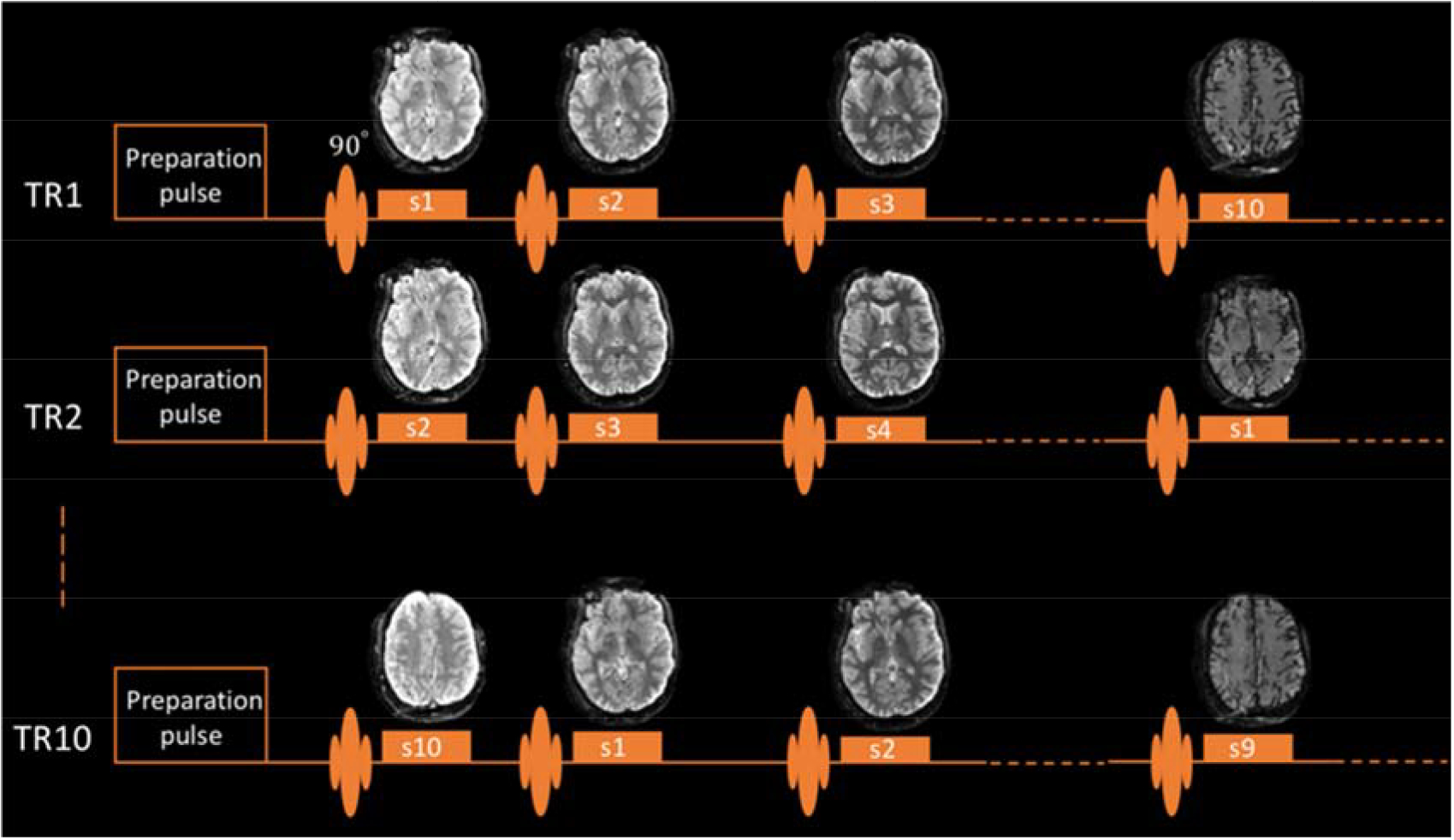
Pulse sequence diagram. One repetition consisting of ten TR cycles is shown. Ten slices were acquired at increasing delays using single-shot EPI, and the slice acquisition order was cycled over TR number.

Table 1.

Parameters used in the IR and ST sequences. TI: inversion time (delay time in the IR experiment); TD: delay time in the ST experiment. ESP: echo spacing; BW: bandwidth.

B0 (T)	Matrix size	Thickness (mm)	Gap (mm)	IR			ST			TE (ms)	Variable TE (ms)	ESP (ms)	BW (kHz)
				TR (ms)	Tis (ms)	Time (min)
0.55	72×54	3	1	4000	10–1200	8.0	3000	8–900	8.0	29	0	0.96	100
1.5	144×108	2	2	5000	10–1400	10.2	4000	9–900	10.8	40	2.20	1.32	132
3	144×108	2	2	6000	9–1600	12.2	4000	9–900	10.8	30	1.15	0.94	250
7	144×108	2	2	6000	8–2000	12.2	4000	7–900	10.8	24	0.48	0.77	250

At all fields, 12 repetitions were performed for IR, including variable TE repetitions and 2 repetitions without inversion pulse as reference (M_0,w). For ST, this number was 16, including 4 reference scans without saturation pulse. An anatomical reference was acquired using a product 3D T₁ -MPRAGE sequence. The in-plane resolution for this scan was two-fold higher than the EPI images. TR, TI, and flip-angle were selected to facilitate successful brain segmentation at each field.

2.3. Data Pre-processing

Image reconstruction was performed using customized code written in IDL (Harris Geospatial Solutions, Boulder, Colorado, USA). A SENSE unfolding matrix was calculated from multi-echo GRE images acquired at the same slice positions and resolution as the EPI images (de Zwart et al., 2002).

Pre-processing of the EPI images included distortion correction, image co-registration, averaging, magnetization polarity correction (for IR data), calculation of saturation levels, and ROI contouring. The procedure was implemented using MATLAB (The MathWorks, Natick, MA) with supplementary image co-registration and segmentation tools in FSL (FMRIB Software Library) (Smith et al., 2004). To correct EPI distortions, B₀ field was first estimated from the multi-echo GRE images, then smoothed by polynomial fitting to the 6^th order. An image-space geometric distortion correction algorithm was implemented based on the smoothed B₀ field and the echo-spacing (ESP) of the EPI images (Jezzard and Balaban, 1995). Image registration was performed using “mcflirt” command in FSL (Jenkinson et al., 2002). Only in-plane registration was performed because of the large gap between slices. Data from different repetitions were then averaged. The binary mask for IR polarity correction was calculated by comparing the image phase of interest and that of the reference image (e.g. data acquired without inversion pulse), thresholded at 1.5 radians. Saturation levels were calculated based on Eq. (2) by dividing the images with RF preparation by the corresponding reference images.

Segmentation of the cortical gray matter (cGM) and three subcortical nuclei (putamen, PU; caudate head, CA; thalamus, TH) on the T₁-MPRAGE images was performed in FSL using “fast” and “first” commands, respectively (Zhang et al., 2001; Patenaude et al., 2011). Anatomical T₁-MPRAGE images at the corresponding slice positions were co-registered in a slice-by-slice manner to the IR images acquired at the similar TI. The same co-registration matrix was applied to the segmentation result. In addition, splenium of corpus callosum (SCC), a homogeneous white matter region, was manually contoured on the IR images. All ROIs were eroded by one pixel to account for potential errors in segmentation, co-registration or distortion correction. The cerebral cortex close to the brain boundary or the sinus was excluded due to sensitivity to signal loss and difficulty for distortion correction. Such ROI adjustments were not performed for the 0.55 T data because of the low resolution and small susceptibility effect.

A representative preprocessing example is shown in Figure 2.

Figure 2.

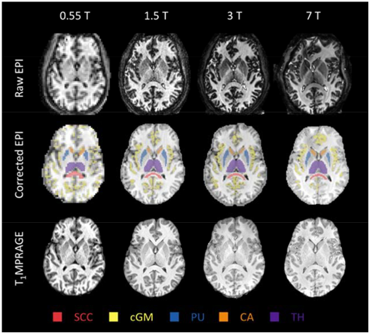
Preprocessing results of a similar slice from a representative subject. Distortion and signal loss in the raw EPI are clearly visible at high fields, which are alleviated in the corrected EPI images. Segmentation results of five ROIs (SCC, splenium of corpus callosum, a homogeneous white matter region; cGM, cortical gray matter; PU, putamen; CA, caudate head; TH, thalamus) are labeled using different colors as indicated in the figure.

2.4. Voxel-based Analysis

At each field, bi-exponential model was fitted to the IR and ST data in a joint fashion using the same relaxation rates but different coefficients

$$\begin{gathered} {\text{S}}_{\text{w},\text{IR}}(t)=a_{\text{s},\text{IR}}{\text{e}}^{-{\lambda }_{\text{s}}t}+a_{\text{f},\text{IR}}{\text{e}}^{-{\lambda }_{\text{f}}t} \\ {\text{S}}_{\text{w},\text{ST}}(t)=a_{\text{s},\text{ST}}{\text{e}}^{-{\lambda }_{\text{s}}t}+a_{\text{f},\text{ST}}{\text{e}}^{-{\lambda }_{\text{f}}t} \end{gathered}$$ (3)

where a_s,IR and a_s,ST correspond to a_s in Eq. (2) for IR and ST, respectively; a_f,IR and a_f,ST correspond to a_f in Eq. (2) for IR and ST, respectively.

Mono- and bi- exponential fittings were also performed on the IR data alone to illustrate their difference, where a_f,IR was free to change in bi-exponential fitting but was fixed to 0 in mono-exponential fitting.

Voxel-wise two-pool analysis using bi-exponential fitting was performed for each subject at 3 and 7 T. It was not performed for the 0.55 and 1.5 T data because a reliable estimate of the fast relaxation component was intractable at these two fields due to their rapid decay and small amplitude compared to the slow component. This notion is illustrated in the results section. For two-pool model fitting, it was assumed that the initial MP pool saturation (at t = 0) in the ST experiment S_m,ST(t = 0) = 0.93, and R_w = 0.40 s⁻¹. The former is based on the numerical simulation of the composite RF pulse and the latter is based on in vivo experimental results, both reported in (van Gelderen et al., 2017). With these assumptions, k_w was calculated as

$$k_{\text{w}}=\frac{\left({\lambda }_{\text{s}}-{\text{R}}_{\text{w}}\right)a_{\text{s},\text{ST}}+\left({\lambda }_{\text{f}}-{\text{R}}_{\text{w}}\right)a_{\text{f},\text{ST}}}{a_{\text{s},\text{ST}}+a_{\text{f},\text{ST}}-{\text{S}}_{\text{m},\text{ST}}(t=0)}$$ (4)

which is derived by substituting S_w,ST(t = 0) = a_s,ST + a_f,ST into the a_s equation in Eq. (2). k_m and R_m were then numerically retrieved by solving the following equations derived from Eq. (2)

$$\begin{gathered} {\lambda }_{\text{f}}+{\lambda }_{\text{s}}={\text{R}}_{\text{w}}+{\text{R}}_{\text{m}}+k_{\text{w}}+k_{\text{m}} \\ {\lambda }_{\text{f}}-{\lambda }_{\text{s}}=\sqrt{{\left({\text{R}}_{\text{w}}-{\text{R}}_{\text{m}}+k_{\text{w}}-k_{\text{m}}\right)}^2+4k_{\text{w}}{k}_{\text{m}}} \end{gathered}$$ (5)

Finally, MP pool fraction f and exchange rate constant k were calculated based on their definitions in Eq. (2).

2.5. ROI-based Analysis

To allow robust fitting at all field strengths, ROI-based analysis was performed. For this purpose, S_IR and S_ST were averaged over voxels in each of the pre-defined ROIs, and jointly fitted to Eq. (3). For IR data from 0.55 and 1.5 T, a_f,IR was set to 0, due to the largely mono-exponential shape of the recovery curve. To calculate the two-pool parameters, white matter and gray matter ROIs were handled differently because of their difference in iron content and thus R_w. The analysis boils down to three steps considering field strength and ROI:

1. High-field (3 and 7 T) analysis in the white matter ROI. The same analysis procedure as the voxel-wise analysis was performed, i.e. Eqs. (4)–(5) were solved assuming S_m,ST(t = 0) = 0.93 and R_w = 0.40 s⁻¹, to yield f, k and R_m.

2. Low-field (0.55 and 1.5 T) analysis in the white matter ROI. Averaged f and k from 7 T were used as a priori knowledge to calculate R_m using the following equation, derived from Eq. (2) using the expression of λ_s

   $${\text{R}}_{\text{m}}=\frac{k_{\text{w}}{k}_{\text{m}}}{{\text{R}}_{\text{w}}+k_{\text{w}}-{\lambda }_{\text{s}}}+{\lambda }_{\text{s}}-k_{\text{m}}$$ (6)

   In this step, R_w was assumed to be 0.40 s⁻¹; No assumption was made about S_m,ST(t = 0).

3. High-field (3 and 7 T) analysis in the gray matter ROIs. Eqs. (4) and (5) were jointly solved to obtain f, k and R_w, with R_m set to the white matter value found at each field strength. This step was not performed for 0.55 and 1.5 T, because it necessitates the use of R_m, which was not independently derived for the corresponding field.

The averaged R_m over subjects at the four fields found in steps 1) and 2) were fitted to a power-law function of B₀ (Korb and Bryant, 2001)

$${\text{R}}_{\text{m}}=a{\text{B}}_0^{-b}$$ (7)

The actual B₀ values of the scanners were calculated from the operating frequencies of the systems as 0.55, 1.50, 2.89 and 6.98 T.

To evaluate the effect of fixing of the parameters S_m,ST(t = 0) and R_w, two-pool analysis of the white matter ROI was repeated at 7 T with parameter values stepped consecutively in the ranges of 0.89–0.97 and 0.3–0.5 s⁻¹, respectively. In addition, R_m was calculated at the four fields using three different fixed R_w values of 0.3, 0.4 and 0.5 s⁻¹, and was fitted separately to the power-law function. The potential effect of k being field dependent (as a result of dipolar cross-relaxation) was also evaluated by linear dependence approximation and calculating the resultant R_m at the low fields.

Linear regression was performed correlating R_w found in step 3) with non-heme iron concentration in the brain structures. The latter was estimated based on a regression model using the ages of the subjects (Hallgren and Sourander, 1958).

Data analysis was performed in MATLAB. Fitting to non-linear equations was performed using “lsqcurvefit” function, and linear regression was based on “regress” function.

3. Results

3.1. Voxel-based Analysis

Transient IR and ST saturation levels are shown in Figure 3. To facilitate comparison across field strengths, a fixed set of TI and TD values was used to generate these images from the voxel-wise bi-exponential fitting parameters. Corresponding source data are shown in Figure S1, and fitting residuals are shown in Figure S2. For IR, a nearly full inversion was achieved at all fields, judged by S_w,IR(t = 0) = a_s,IR + a_f,IR ≈ 2 (1.97±0.03, 1.96±0.04, 1.96±0.04, 1.96±0.05 for 0.55, 1.5, 3 and 7 T, respectively). CSF appears dark due to long T₁ and incomplete recovery at the given TR. Consistent T₁ contrast is observed at all fields, and, as expected, the relaxation rate decreases as field strength increases. For ST, S_w,ST(t = 0) = a_s,IR + a_f,IR ≈ 0 (0.02±0.01, 0.03±0.02, 0.02±0.03, 0.04±0.03 for 0.55, 1.5, 3 and 7 T, respectively), indicating that the water signal is not significantly affected by the saturation pulse. The MT effect becomes increasingly stronger in intensity and longer in duration with increasing field strength.

Figure 3.

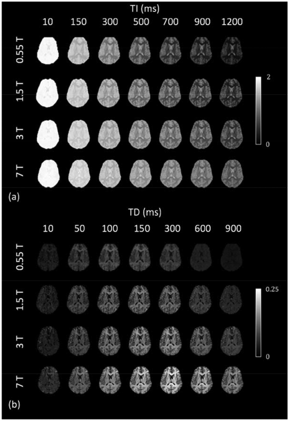
Evolution of water magnetization disturbance (S_w,IR and S_w,ST in Eq. (3)) after IR (a) and ST (b) pulse for each of the four field strengths. Images were generated corresponding to a fixed set of delays after voxel-wise bi-exponential fitting, since the actual delays were not the same at the four fields.

A comparison of mono- and bi-exponential fitting to the IR data is shown in Figure 4 and Figure S3. Both methods lead to similar T₁ images; However, the mono-exponential fitting residuals at 3 and 7 T are significantly larger compared to those at 0.55 and 1.5 T especially in the white matter, indicating the presence of an additional component, which can be well described using bi-exponential fitting judged by the much smaller residuals. At 0.55 T, the elevated fitting residuals in CSF is attributed to long T₁ and incomplete recovery at the given TR that changes the shape of the signal evolution. Partial volume effects on the ventricle boundary also contributes to the large residuals, as the IR polarity correction cannot be properly performed with the mixed tissues having different signal null times (ln2 ∙ T₁, when M_z,w(t) becomes 0).

Figure 4.

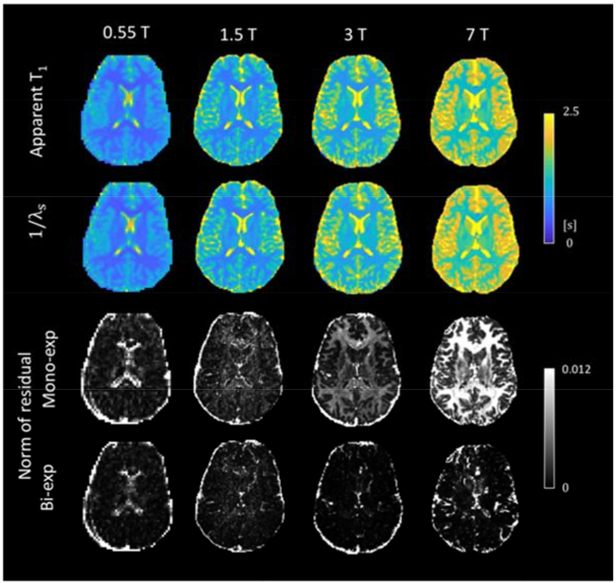
Mono- and bi-exponential fitting for the IR data. (a) Apparent T₁ maps using mono-exponential fitting and 1/λ_s maps from the bi-exponential fitting. (b) Second norm of the residual vector using the two fitting methods.

Two-pool fitting results from 3 and 7 T are shown in Figure 5. Consistent k and f maps are obtained at the two fields, with those from 3 T being noisier due to the lower SNR compared to 7 T. Strong contrast is observed between gray and white matter for both f and k, while contrast within white matter is rather modest. R_m is spatially rather homogeneous across both white matter and cortical gray matter, yet a significant global difference is observed between 3 and 7 T.

Figure 5.

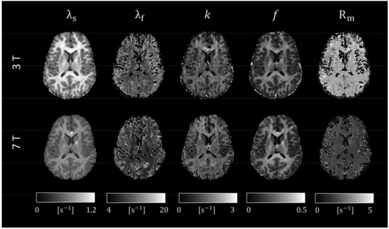
Relaxation rates and two-pool parameters at 3 and 7 T.

3.2. White Matter ROI-analysis with Fixed R_w

The time evolutions of S_w,IR and S_w,ST in the white matter ROI, as well as the bi-exponential fitting results, are shown in Figure 6. The data traces are clearly field-dependent, and they are all well fitted by the model (R²>0.999 for all curves). Similarly high-quality fits are found for the other ROIs (Figure S4). The statistics of the fitted parameters are summarized in Table S2.

Figure 6.

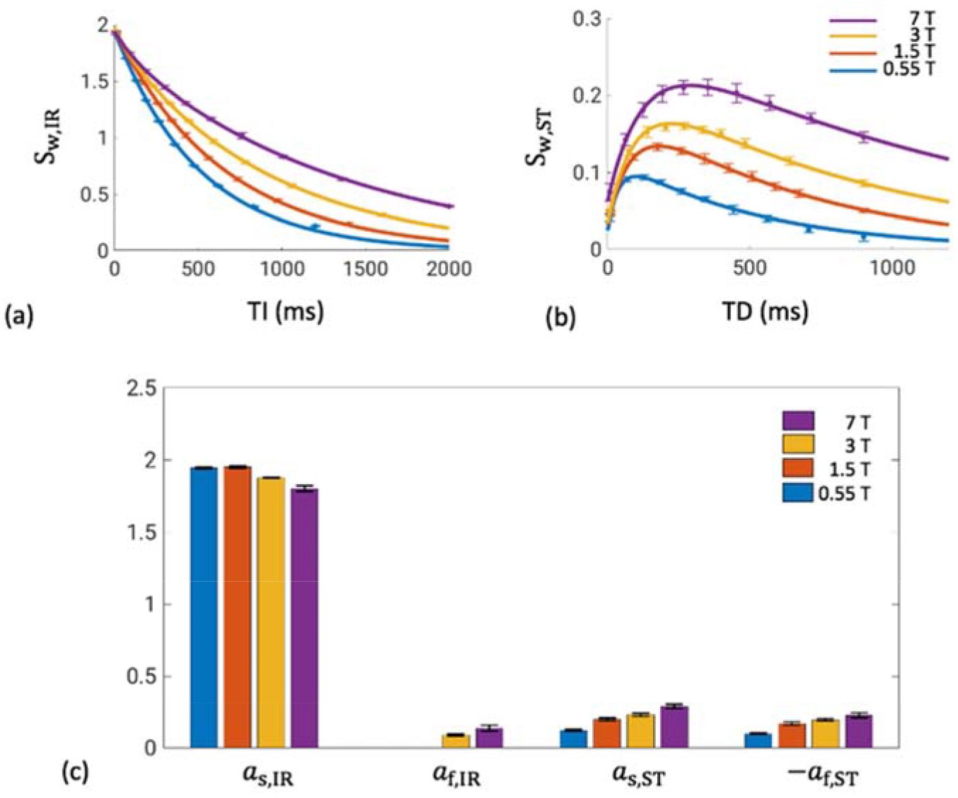
Transient IR (a) and ST (b) signals in the white matter ROI (SCC), and the fitting parameters in the bi-exponential model (c). Data is shown as mean ± standard deviation over subjects. (a) and (b), solid lines denote fitting to the mean values. (c) a_f,IR was set to 0 at 0.55 and 1.5 T, as described in the methods. See Table S2 for the statistics.

Two-pool analysis results of the white matter ROI are summarized in Table 2. Tissue-specific parameters obtained from 3 and 7 T are consistent with each other: a relative difference of 3.2% was found in f and 8.0% in k between the two fields. These values are close to those reported in (van Gelderen et al., 2016), in which f was found to average at 0.268 and k at 1.50 s⁻¹ at 7 T over ten healthy volunteers. A substantial difference of 52.4% is obtained between R_m from the two fields, which leads to the difference observed in λ. Using the mean f and k values from 7 T, R_m in the white matter SCC at 1.5 T and 0.55 T is calculated as 8.2 ± 0.5 s⁻¹ and 22.8 ± 2.6 s⁻¹ across subjects, respectively. R_m values from the four fields are fitted well by R_m = 12.2B₀ ^−1.00 with R² =0.997 (Figure 7).

Table 2.

Bi-exponential fitting and two-pool analysis results of white matter SCC at 3 and 7 T. Data is shown as mean ± standard deviation over subjects. λ, R and k are reported in s⁻¹.

B0	λs	λf	Rw	Rm	Sm_SR(t = 0)	f	k
3 T	1.112 ± 0.025	10.60 ± 0.40	0.40 (Fixed)	3.89 ± 0.07	0.93 (Fixed)	0.281 ± 0.014	1.50 ± 0.05
7 T	0.760 ± 0.008	8.19 ± 0.37	0.40 (Fixed)	1.85 ± 0.09	0.93 (Fixed)	0.289 ± 0.017	1.38 ± 0.09

Figure 7.

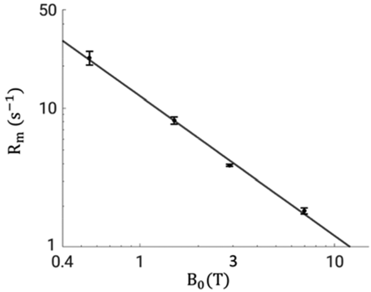
Log-log plot of the B₀ dependence of R_m. Data is shown as mean ± standard deviation over subjects. Solid black line denotes the fit to the means using a power-law function R_m = 12.2B₀ ^−1.00 (R²=0.997). 95% confidence intervals for the fit parameters are: [11.7, 12.6] for a (amplitude); [−1.03, −0.96] for −b (exponent).

Based on Eq. (2), the power-law function of R_m and the two-pool parameters found at 7 T, λ_f is estimated to be 13.7 s⁻¹ and 27.3 s⁻¹ at 1.5 T and 0.55 T, respectively. Further assuming S_w,IR(t = 0) = 2 and S_m,IR(t = 0) = 0.9 after the hyperbolic inversion pulse, a_f,IR is estimated to be −0.01 and −0.04 at 1.5 T and 0.55 T, respectively, in contrast to a_s,IR ≈ S_w,IR(t = 0) = 2. These estimates support the notion that the contribution of the fast IR component is negligible at these two fields.

3.3. Effects of Fixed Parameters in White Matter

Modification of the assumed R_w and S_m,ST(t = 0) values mildly changes R_m, f and k results as demonstrated using the 7 T data in Table 3 and Table 4. Using a different R_w value of 0.3 or 0.5 s⁻¹ moderately changes R_m at the four fields, yet the power-law dependence is preserved judged by the high R² values.

Table 3.

Evaluation of the assumed S_m,ST(t = 0) values to the two-pool parameters at 7 T and the corresponding fit to the power-law function. R_w is fixed at 0.40 s⁻¹. Data is shown as mean ± standard deviation over eight subjects. R²>0.99 for all fits.

Assumed Sm,ST(t = 0)	Rm (s−1)	f	k (s−1)	Rm=aB0−b
0.89	1.78±0.08	0.300±0.018	1.42±0.09	Rm = 10.5Bo−0.93
0.91	1.82±0.09	0.295±0.018	1.40±0.09	Rm = 11.3B0−0.96
0.93	1.85±0.09	0.289±0.017	1.38±0.09	Rm = 12.2B0−1.00
0.95	1.88±0.09	0.284±0.017	1.35±0.09	Rm = 13.2B0−1.04
0.97	1.92±0.09	0.279±0.017	1.33±0.09	Rm = 14.4B0−1.08

Table 4.

Evaluation of the assumed R_w values to the two-pool parameters at 7 T and the corresponding fit to the power-law function. S_m,ST(t = 0) is fixed at 0.93. Data is shown as mean ± standard deviation over eight subjects. R²>0.98 for all fits.

Assumed Rw (s−1)	Rm (s−1)	f	k (s−1)	Rm=aB0−b
0.30	2.18±0.12	0.299±0.017	1.35±0.09	Rm = 15.5B0−1.07
0.35	2.02±0.10	0.294±0.017	1.36±0.09	Rm = 13.6B0−1.02
0.40	1.85±0.09	0.289±0.017	1.38±0.09	Rm = 12.2B0−1.00
0.45	1.69±0.07	0.285±0.018	1.39±0.09	Rm = 11.0Bo−0.98
0.50	1.53±0.06	0.281±0.017	1.40±0.09	Rm = 10.0B0−0.97

With the assumed linear B₀ dependence of k (i.e., 1.54 s⁻¹ at 1.5 T and 1.57 s⁻¹ at 0.55 T based on k from 3 and 7 T data), the resultant R_m in the white matter SCC at 1.5 and 0.55 T are 7.3 ± 0.4 s⁻¹ and 15.4 ± 2.6 s⁻¹, and the power-law fitting leads to R_m = 9.6B₀ ^−0.84 with R²=0.998.

3.4. ROI-based Analysis Using Fixed ;_I at 3 and 7 T

ROI-based analysis results for 3 and 7 T data with R_m fixed to the values reported in Table 2 are shown in Figure 8. Good correspondence of the resulting f values between the two fields is observed for all ROIs. Data points are clustered based on ROI. Notably, white matter SCC has higher f value than all of the gray matter structures, consistent with its higher myelin content. The clustering behavior is less prominent for k values, yet SCC shows higher k compared to other ROIs.

Figure 8.

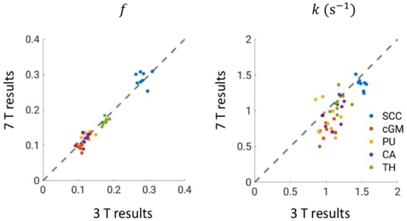
Comparison of two-pool analysis results at 3 and 7 T using fixed R_m values. The mean values inside ROIs for each subject are shown; The identity line is shown as dashed. Refer to Table S2 for the statistics of f and k in each ROI.

Figure 9 shows a clear linear increase of R_w with tissue non-heme iron concentration at both fields, yet the dependence is weak as judged by the small slope. This is in agreement with a previous study using multiple linear regression (Rooney et al., 2007). Indeed, analyzing our data using this same approach, we found similar fitting parameters (Figure S5). Nevertheless, a somewhat smaller contribution of iron to R_w is observed at 7 T compared to 3 T in our data, which may have come from a bias introduced by selective signal loss due to the shorter T₂ * at 7 T.

Figure 9.

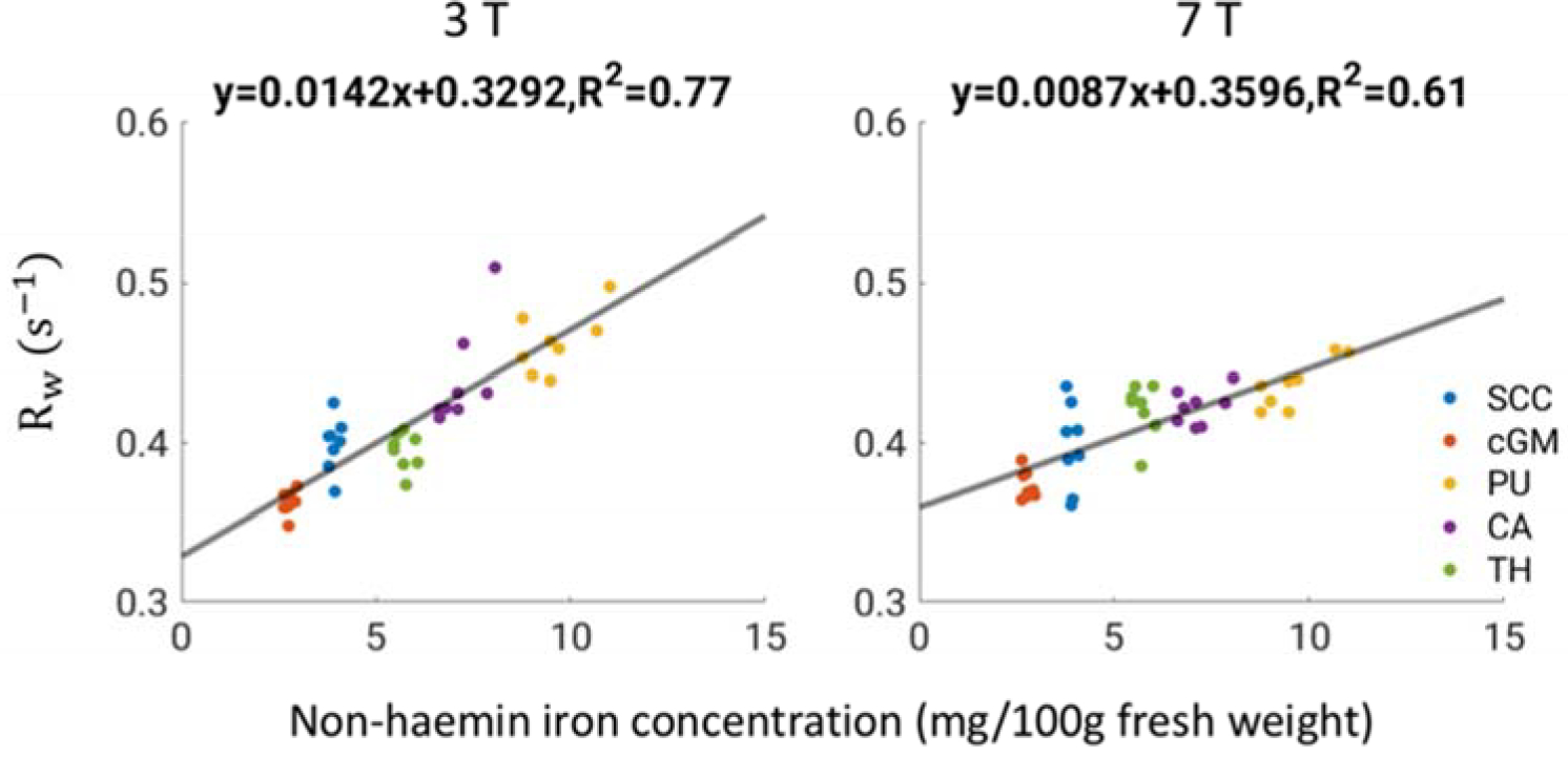
Correlation of R_w and non-heme iron concentration at 3 and 7 T. Data points denote values from each subject. Black lines denote linear fitting results of the data. 95% confidence intervals for the fit parameters are: [0.0116, 0.0167] for 0.0142; [0.3131, 0.3453] for 0.3292; [0.0064, 0.0110] for 0.0087; [0.3453, 0.3739] for 0.3596.

4. Discussion

Using joint analysis of IR and ST data acquired in the healthy human brain at four magnetic field strengths from 0.55 to 7 T, we have shown that tissue R₁ (T₁) dependence on magnetic field strength in large part can be explained by a field-dependent relaxation rate of macromolecular protons R_m. Analysis of the measurements with a two-pool exchange model showed that R_m depends on field strength approximately in an inverse linear fashion. Based on the calculated R_m values, tissue-specific parameters f, k, R_w in various brain structures were measured at 3 and 7 T. f, k results are consistent at the two fields; R_w showed a clear linear correlation with tissue iron concentration.

The present study was designed to further the understanding of tissue T₁ contrast in the human brain in the context of the wide range of field strengths employed in clinical practice and neuroscientific research. This goal was achieved by separating contributions of the field-dependent R_m from the relatively stable R_m in the white matter based on the two-pool model. In comparison with quantitative T₁ as a single biomarker, multi-compartment models yield parameters with physiologically relevant origins, which may facilitate the interpretation of tissue T₁ particularly in disease.

4.1. Field Dependence of R_m

Based on analysis of one of the major fiber bundles in the brain, the splenium of the corpus callosum (SCC), we established a power-law dependence of the myelin proton relaxivity in the form of R_m = 12.2B₀ ^−1.00. The 1.00 magnitude of the exponent exceeds the range of 0.5 – 0.85 reported in NMR studies of chain-like macromolecules (Nusser and Kimmich, 1990; Korb and Bryant, 2002). There are various potential contributors to this discrepancy. First, the previous experiments were performed on hydrated protein and polypeptide at room temperature and below, conditions quite different from the current study. Secondly, previous measurements on chain molecules were based on fast field-cycling spectrometer operating at Larmor frequencies below 30 MHz, while the frequencies studied here were mostly substantially higher at 23, 64, 128 and 298 MHz. Considering the complicated magnetic dispersion curve observed in biological tissues (Duvvuri et al., 2001; Araya et al., 2017), some change in the power-law across this large frequency range is to be expected. Third, the assumed two-pool parameters, i.e. f, k, R_w and initial saturation conditions, are significantly variable across studies, which eventually make contributions to the variability in R_m. Fourth, while the power law may apply generally to chain molecules with restricted motion, the value of the exponent will depend on the molecular species and physical conditions. For example, and relevant for the current findings, a close to linear frequency dependence has been predicted and observed in a study of smectic lipid bilayers (Kimmich and Voigt, 1979; Rommel et al., 1988; Kimmich and Anoardo, 2004). Previously found R_m values in NMR studies of lipid protons are also consistent with this (Lee et al., 1972; McLaughlin et al., 1973; Ellena et al., 1985).

Lastly, and importantly, other mechanisms may contribute to T₁ relaxation. Our model of brain tissue T₁ being dominated by paramagnetic sources such as iron, and by magnetization exchange with lipid, is necessarily overly simplistic and ignores other likely contributors. The most important ones among these may be the influence of water of reduced mobility near the surface of large molecules (such as lipid in myelin) (Diakova et al., 2012). Indeed, molecular dynamics simulation of a myelin layer segment (Schyboll et al., 2019) indicates an increase of R_m near lipid headgroups; However, the effect drops significantly within 1 nm from the interaction surface and the overall effect to the free water pool is small. Therefore, interfacial water alone appears insufficient to account for as much as 30% of the total spins (f in the two-pool model) with a linearly field dependent R_m. Thus, while simplistic, the two-pool model may be a good approximation to T₁ relaxation effects in brain tissue, specifically its field dependence in white matter.

In the current study, SCC was analyzed as a representative white matter region. It was chosen because of its well-defined shape and the excellent homogeneity over a sufficiently large volume, which improves measurement consistency across scanners as well as across subjects. Analyses in other white matter regions have been attempted, yet significant inconsistency in R_m was observed, presumably driven by the spatial heterogeneity of white matter. In part, this may have been caused by variations in k originating from the spatial variation in myelin thickness (Aboitiz et al., 1992). Indeed, it has been noticed that some of the T₁ heterogeneity across white matter correlates with local microstructure (Harkins et al., 2016; Lee et al., 2018). Reasonable consistency was achieved when analyzing signals averaged across the white matter, which led to R_m of 25.0±4.0, 9.0±0.5, 3.99±0.05, 1.90±0.05 s⁻¹ at 0.55, 1.5, 3 and 7 T, respectively. A fit of R_m = 13.2B₀ ^−1.03 was found with R²=0.996, similar to the results in the SCC.

4.2. Projection of Tissue T₁ to Higher Fields

Assuming the extendability of the power-law dependence between R_m and the field strength up to 14 T, based on the two-pool parameters found at 7 T, estimated time constants T₁ for the slow component at 9.4, 10.5, 11.7 and 14.0 T (Larmor frequencies 400, 447, 498 and 596 MHz) are 1.57, 1.66, 1.74, and 1.89 s in the white matter SCC, and 2.22, 2.27, 2.32, and 2.41 s in the cortex.

There are several potential caveats of this projection. First, as indicated above, the diversity of MP species in tissue and the complex frequency spectrum of possible MP motions may result in a complex B₀ dependence that cannot be fully described by the simple power-law, similar to that in the low end of the field (Knispel et al., 1974). Secondly, it is likely but not certain that R_w remains mildly field-dependent at ultra-high fields. Potential modifiers of R_m include contributions from interfacial water and water near paramagnetic ions. If this assumption is violated, the unaccounted R_w change should be considered in the model. Based on the formulae of λ in Eq. (2), it is estimated that $\frac{\partial {\lambda }_{\text{s}}}{\partial {\text{R}}_{\text{w}}}\approx 0.41$ and $\frac{\partial {\lambda }_{\text{f}}}{\partial {\text{R}}_{\text{w}}}\approx 1.59$ using the 7 T data in the white matter SCC.

4.3. Comparison to Quantitative Magnetization Transfer Methods

The macromolecular proton fraction f of several brain ROIs was estimated in the two-pool analysis, which is a target biomarker in quantitative Magnetization Transfer (qMT) experiments. In vivo qMT methods can be generally classified into two categories: pulsed Z-spectrum (Graham and Henkelman, 1997; Sled and Pike, 2001; Yarnykh, 2002), and on-resonance cross-relaxometry (Chai et al., 1996; Gochberg et al., 1997; Dortch et al., 2013b). The former involves RF pulses with variable off-resonance frequency and power to depict the macromolecular spectrum, and the latter is based on on-resonance pulses that differentially saturate the two pools. Both IR and ST experiments in this study fall into the second category.

Compared to the pulsed Z-spectrum methods, on-resonance cross-relaxometry does not provide macromolecular absorption lineshape, but it has advantages concerning RF power (or Specific Absorption Rate, SAR) constraints, which is increasingly relevant for applications at ultra-high fields. Among the on-resonance cross-relaxometry methods, there are a few interesting similarities and differences between our method and the Selective Inversion Recovery (SIR) method recently reported at 7 T (Dortch et al., 2013b). Both methods are based on observation of transient signal after an RF pulse that differentially saturates the two pools. In SIR, a carefully designed low-power inversion pulse is applied to invert water magnetization while minimizing MP saturation. Due to the strong ${\text{B}}_1^{+}$ inhomogeneity encountered at 7 T, the exact spatial distribution of MP saturation needs to be estimated by simulation using measured ${\text{B}}_1^{+}$ and an assumed macromolecular lineshape. In contrast, the current study uses a high-power adiabatic inversion pulse to invert water signal and fully saturate MP, and a high-power ST pulse aimed to fully saturate MP while minimizing water saturation. The short high-power pulses used in this study are less sensitive to B₀ and ${\text{B}}_1^{+}$ inhomogeneity, as well as the underlying macromolecular lineshape. In addition, both methods require a mechanism to “reset” the magnetizations before the next TR. In SIR, this is achieved by saturating both pools using a high-power hard-pulse train, while in the current study this is achieved with a long TR for the magnetization to recover to thermal equilibrium.

In the current study, we found f in the SCC to average 0.289 at 7 T, which corresponds to a macromolecular to free pool size ratio (PSR) of 0.406, as typically reported in qMT studies. This value is substantially higher than previous qMT studies (Sled and Pike, 2001; Yarnykh, 2002; Dortch et al., 2013b). While this discrepancy may be partially attributed to the fixed R_m value of ~ 1 s⁻¹ used in previous studies regardless of B₀ (Helms and Hagberg, 2009), contributing factors remain incompletely understood and require further investigation.

4.4. Contribution of Iron to T₁

Using joint analysis of MRI and an element-specific imaging technique PIXE, Stüber et al. reported a substantially higher relative contribution of iron to R₁ in the gray matter than white matter (Stüber et al., 2014). Therefore, it is necessary to account for the iron concentration when quantifying cortical myelin using R₁ (T₁). Our results suggest that the increasing effects of iron to tissue R₁ may be modeled by a proportionally increased R_w. This finding may be exploited to separate the synergistic influence of myelin and iron to R₁ in cortical myelin mapping. Nevertheless, caution needs to be taken when analyzing subcortical gray matter, as the concomitant impact of iron on T₂ * becomes significant and may disrupt the linear relationship found between iron and observed R_w.

Rooney et al. (Rooney et al., 2007) utilized a multiple linear model of iron level and macromolecular content to fit tissue apparent R₁. In comparison, the current work disentangles iron and MP contributions to R₁ by modeling their separate effect on R_w and R_m, respectively. One may also consider iron’s contribution to R_m, yet this effect on R₁ should be relatively small, in part because the MP fraction is smaller than the WP fraction, and secondly because most of the MP will not be within the close distance to iron required for the T₁ relaxation mechanism (Möller et al., 2019).

4.5. Technical Limitations

In the following we discuss a few technical limitations of this study, which may have contributed more significantly than others to the measurement inaccuracies.

First of all, the two-pool model is the simplest multi-compartment model, which may not adequately capture the relevant features of T₁ relaxation in human tissue. For example, the myelin sheath has a complex multi-layer structure that traps approximately 15–20% of the total free water in the white matter (Norton and Cammer, 1984; Mackay et al., 1994). The trapped water has NMR properties distinct from those of interstitial water (water outside the axons), including resonance frequency and longitudinal and transverse relaxation rates. Distinguishing different water pools by modeling interstitial water and myelin water separately may improve the accuracy of results (Stanisz et al., 1999; Kalantari et al., 2011; Dortch et al., 2013a). Furthermore, diffusion of myelin water between different layers may be described using a cascaded multi-compartment model together with their corresponding macromolecular pools, a more realistic model of the multi-layer structure of the myelin sheath (van Gelderen and Duyn, 2019). Improved accuracy may also be possible when splitting the MP pool between myelin or non-myelin protons or between lipid or protein protons. These MP species may possess intrinsically different relaxation properties and sensitivity to neuro-degenerative diseases. Nevertheless, increasing model complexity, while offering potentially increased accuracy, will also likely decrease fitting convergence and robustness.

Another limitation is the choice of a relatively short repetition time (TR) to keep the overall experimental time reasonable. The 3–6 s range chosen here were hardly sufficient to allow full recovery of the longitudinal magnetization, somewhat affecting the model fitting. Effect of incomplete recovery can be observed in Figure 3 from both IR and ST, as analyzed in the corresponding results section. In addition, due to the slice-delay time cycling nature of the sequence, the effective TR (nominal TR minus delay time) varies from slice to slice, which slightly modifies the shape of the saturation curves. Using Bloch simulation, it is estimated that the relative errors in λ_s and λ_f due to the use of finite TRs in the experiments are 1.58% and 5.85%, respectively (Supplementary Information). Advanced models that consider the finite TR and timing differences of slices are currently under investigation which may yield improved accuracy.

A third technical limitation is the use of EPI for image acquisition. The long signal acquisition time and TE (about 50 and 30 ms respectively) necessarily lead to substantial T₂ * weighting, reducing the relative signal contribution of protons in close proximity of iron and macromolecules. For this reason, the contribution of myelin water, with its short T₂ *, was likely small in our experiments. Also, because of this strong T₂ * weighting, signal in an iron-rich region such as the Globus Pallidus (T₂ * of about 12 and 25 ms at 7 T and 3 T respectively (Yao et al., 2009)) was small and too unreliable to allow model fitting. This varying T₂ * weighting may have affected the slopes found with R_w fitting to iron level at 3 and 7 T (Figure 9). Meanwhile, the B₀ field in the human brain has high-order spatial terms associated with air cavities near brain tissue and susceptibility variations across brain tissues whose strengths scale with B₀ and are sensitive to head pose and motion (Liu et al., 2018). To mitigate the effect of T₂ * on T₁ estimation, one potential approach might be to use multi-echo GRE for signal readout to capture the fast-decaying signal right after excitation. Combined with different preparation RF pulses and multi-component analysis, multi-echo GRE readout may also improve the specificity of proton species detection by enabling analysis of more complicated and physiologically relevant models, such as a multi-layer model of the myelin (van Gelderen and Duyn, 2019).

5. Conclusions

Joint two-pool model analysis of inversion recovery and saturation transfer data at clinical field strengths ranging from 0.55 to 7 T suggests that B₀ field-dependence of the macromolecular proton longitudinal relaxation rate R_m in the white matter follows a simple inverse linear function R_m = 12.2/B₀, a special case of the more generally applied power-law relationship R_m = aB₀ ^–b found in previous NMR studies. Assuming the general applicability of this power-law function to gray matter structures, tissue specific parameters such as macromolecular proton fraction and magnetization exchange rate are found to be consistent among subjects and between 3 and 7 T. In tissues with high iron content, e.g. the basal ganglia, or pathological iron accumulation, ROI-based averaging appears required to allow separation of the effects of iron and myelin on T₁.

References

- Aboitiz F, Scheibel AB, Fisher RS, Zaidel E, 1992. Fiber composition of the human corpus callosum. Brain Research 598, 143–153. 10.1016/0006-8993(92)90178-C [DOI] [PubMed] [Google Scholar]
- Araya YT, Martínez-Santiesteban F, Handler WB, Harris CT, Chronik BA, Scholl TJ, 2017. Nuclear magnetic relaxation dispersion of murine tissue for development of T1 (R1) dispersion contrast imaging. NMR in Biomedicine 30, e3789 10.1002/nbm.3789 [DOI] [PubMed] [Google Scholar]
- Bryant RG, Mendelson DA, Lester CC, 1991. The magnetic field dependence of proton spin relaxation in tissues. Magnetic Resonance in Medicine 21, 117–126. 10.1002/mrm.1910210114 [DOI] [PubMed] [Google Scholar]
- Campbell-Washburn AE, Ramasawmy R, Restivo MC, Bhattacharya I, Basar B, Herzka DA, Hansen MS, Rogers T, Bandettini WP, McGuirt DR, Mancini C, Grodzki D, Schneider R, Majeed W, Bhat H, Xue H, Moss J, Malayeri AA, Jones EC, Koretsky AP, Kellman P, Chen MY, Lederman RJ, Balaban RS, 2019. Opportunities in Interventional and Diagnostic Imaging by Using High-Performance Low-Field-Strength MRI. Radiology 293, 384–393. 10.1148/radiol.2019190452 [DOI] [PMC free article] [PubMed] [Google Scholar]
- Chai J-W, Chen C, Chen JH, Lee S-K, Yeung HN, 1996. Estimation of in vivo proton intrinsic and cross-relaxation rates in human brain. Magnetic Resonance in Medicine 36, 147–152. 10.1002/mrm.1910360123 [DOI] [PubMed] [Google Scholar]
- Chan SI, Feigenson GW, Seiter CHA, 1971. Nuclear Relaxation Studies of Lecithin Bilayers. Nature 231, 110–112. 10.1038/231110a0 [DOI] [PubMed] [Google Scholar]
- de Zwart JA, Ledden PJ, Kellman P, Gelderen P van, Duyn JH, 2002. Design of a SENSE-optimized high-sensitivity MRI receive coil for brain imaging. Magnetic Resonance in Medicine 47, 1218–1227. 10.1002/mrm.10169 [DOI] [PubMed] [Google Scholar]
- Deese AJ, Dratz EA, Hymel L, Fleischer S, 1982. Proton NMR T1, T2, and T1 rho relaxation studies of native and reconstituted sarcoplasmic reticulum and phospholipid vesicles. Biophysical Journal 37, 207–216. 10.1016/S0006-3495(82)84670-5 [DOI] [PMC free article] [PubMed] [Google Scholar]
- Deoni SCL, Peters TM, Rutt BK, 2005. High-resolution T1 and T2 mapping of the brain in a clinically acceptable time with DESPOT1 and DESPOT2. Magnetic Resonance in Medicine 53, 237–241. 10.1002/mrm.20314 [DOI] [PubMed] [Google Scholar]
- Diakova G, Korb J-P, Bryant RG, 2012. The magnetic field dependence of water T1 in tissues. Magnetic Resonance in Medicine 68, 272–277. 10.1002/mrm.23229 [DOI] [PMC free article] [PubMed] [Google Scholar]
- Dick F, Tierney AT, Lutti A, Josephs O, Sereno MI, Weiskopf N, 2012. In Vivo Functional and Myeloarchitectonic Mapping of Human Primary Auditory Areas. J. Neurosci 32, 16095–16105. 10.1523/JNEUROSCI.1712-12.2012 [DOI] [PMC free article] [PubMed] [Google Scholar]
- Dixon WT, 1984. Simple proton spectroscopic imaging. Radiology 153, 189–194. 10.1148/radiology.153.1.6089263 [DOI] [PubMed] [Google Scholar]
- Dortch RD, Harkins KD, Juttukonda MR, Gore JC, Does MD, 2013a. Characterizing intercompartmental water exchange in myelinated tissue using relaxation exchange spectroscopy: REXSY in Optic and Sciatic Nerve. Magnetic Resonance in Medicine 70, 1450–1459. 10.1002/mrm.24571 [DOI] [PMC free article] [PubMed] [Google Scholar]
- Dortch RD, Moore J, Li K, Jankiewicz M, Gochberg DF, Hirtle JA, Gore JC, Smith SA, 2013b. Quantitative magnetization transfer imaging of human brain at 7T. NeuroImage 64, 640–649. 10.1016/j.neuroimage.2012.08.047 [DOI] [PMC free article] [PubMed] [Google Scholar]
- Duvvuri U, Goldberg AD, Kranz JK, Hoang L, Reddy R, Wehrli FW, Wand AJ, Englander SW, Leigh JS, 2001. Water magnetic relaxation dispersion in biological systems: The contribution of proton exchange and implications for the noninvasive detection of cartilage degradation. PNAS 98, 12479–12484. 10.1073/pnas.221471898 [DOI] [PMC free article] [PubMed] [Google Scholar]
- Edzes HT, Samulski ET, 1977. Cross relaxation and spin diffusion in the proton NMR of hydrated collagen. Nature 265, 521–523. 10.1038/265521a0 [DOI] [PubMed] [Google Scholar]
- Ellena JF, Hutton WC, Cafiso DS, 1985. Elucidation of cross-relaxation pathways in phospholipid vesicles utilizing two-dimensional proton NMR spectroscopy. J. Am. Chem. Soc 107, 1530–1537. 10.1021/ja00292a013 [DOI] [Google Scholar]
- Eng J, Ceckler TL, Balaban RS, 1991. Quantitative 1H magnetization transfer imaging in vivo. Magnetic Resonance in Medicine 17, 304–314. 10.1002/mrm.1910170203 [DOI] [PubMed] [Google Scholar]
- Forsén S, Hoffman RA, 1963. Study of Moderately Rapid Chemical Exchange Reactions by Means of Nuclear Magnetic Double Resonance. The Journal of Chemical Physics 39, 2892–2901. 10.1063/1.1734121 [DOI] [Google Scholar]
- Glasser MF, Essen DCV, 2011. Mapping Human Cortical Areas In Vivo Based on Myelin Content as Revealed by T1- and T2-Weighted MRI. J. Neurosci 31, 11597–11616. 10.1523/JNEUROSCI.2180-11.2011 [DOI] [PMC free article] [PubMed] [Google Scholar]
- Gochberg DF, Kennan RP, Gore JC, 1997. Quantitative studies of magnetization transfer by selective excitation and T1 recovery. Magnetic Resonance in Medicine 38, 224–231. 10.1002/mrm.1910380210 [DOI] [PubMed] [Google Scholar]
- Gossuin Y, Roch A, Muller RN, Gillis P, 2000. Relaxation induced by ferritin and ferritin-like magnetic particles: The role of proton exchange. Magnetic Resonance in Medicine 43, 237–243. [DOI] [PubMed] [Google Scholar]
- Graham SJ, Henkelman RM, 1997. Understanding pulsed magnetization transfer. Journal of Magnetic Resonance Imaging 7, 903–912. 10.1002/jmri.1880070520 [DOI] [PubMed] [Google Scholar]
- Hallgren B, Sourander P, 1958. The Effect of Age on the Non-Haemin Iron in the Human Brain. Journal of Neurochemistry 3, 41–51. 10.1111/j.1471-4159.1958.tb12607.x [DOI] [PubMed] [Google Scholar]
- Harkins KD, Xu J, Dula AN, Li K, Valentine WM, Gochberg DF, Gore JC, Does MD, 2016. The microstructural correlates of T1 in white matter. Magnetic Resonance in Medicine 75, 1341–1345. 10.1002/mrm.25709 [DOI] [PMC free article] [PubMed] [Google Scholar]
- Helms G, Hagberg GE, 2009. In vivo quantification of the bound pool T1 in human white matter using the binary spin–bath model of progressive magnetization transfer saturation. Phys. Med. Biol 54, N529–N540. 10.1088/0031-9155/54/23/N01 [DOI] [PubMed] [Google Scholar]
- Henkelman RM, Huang X, Xiang Q-S, Stanisz GJ, Swanson SD, Bronskill MJ, 1993. Quantitative interpretation of magnetization transfer. Magnetic Resonance in Medicine 29, 759–766. 10.1002/mrm.1910290607 [DOI] [PubMed] [Google Scholar]
- Jenkinson M, Bannister P, Brady M, Smith S, 2002. Improved Optimization for the Robust and Accurate Linear Registration and Motion Correction of Brain Images. NeuroImage 17, 825–841. 10.1006/nimg.2002.1132 [DOI] [PubMed] [Google Scholar]
- Jezzard P, Balaban RS, 1995. Correction for geometric distortion in echo planar images from B0 field variations. Magnetic Resonance in Medicine 34, 65–73. 10.1002/mrm.1910340111 [DOI] [PubMed] [Google Scholar]
- Jiang X, van Gelderen P, Duyn JH, 2017. Spectral characteristics of semisolid protons in human brain white matter at 7 T. Magnetic Resonance in Medicine 78, 1950–1958. 10.1002/mrm.26594 [DOI] [PMC free article] [PubMed] [Google Scholar]
- Kalantari S, Laule C, Bjarnason TA, Vavasour IM, MacKay AL, 2011. Insight into in vivo magnetization exchange in human white matter regions. Magnetic Resonance in Medicine 66, 1142–1151. 10.1002/mrm.22873 [DOI] [PubMed] [Google Scholar]
- Kanda T, Ishii K, Kawaguchi H, Kitajima K, Takenaka D, 2013. High Signal Intensity in the Dentate Nucleus and Globus Pallidus on Unenhanced T1-weighted MR Images: Relationship with Increasing Cumulative Dose of a Gadolinium-based Contrast Material. Radiology 270, 834–841. 10.1148/radiol.13131669 [DOI] [PubMed] [Google Scholar]
- Kimmich R, Anoardo E, 2004. Field-cycling NMR relaxometry. Progress in Nuclear Magnetic Resonance Spectroscopy 44, 257–320. 10.1016/j.pnmrs.2004.03.002 [DOI] [PubMed] [Google Scholar]
- Kimmich R, Voigt G, 1979. Nuclear magnetic relaxation dispersion in lecithin bilayers. Chemical Physics Letters 62, 181–183. 10.1016/0009-2614(79)80438-8 [DOI] [Google Scholar]
- Kingsley PB, 1999. Methods of measuring spin-lattice (T1) relaxation times: An annotated bibliography. Concepts in Magnetic Resonance 11, 243–276. [DOI] [Google Scholar]
- Knispel RR, Thompson RT, Pintar MM, 1974. Dispersion of proton spin-lattice relaxation in tissues. Journal of Magnetic Resonance (1969) 14, 44–51. 10.1016/0022-2364(74)90255-8 [DOI] [Google Scholar]
- Koenig SH, Brown RD, Spiller M, Lundbom N, 1990. Relaxometry of brain: Why white matter appears bright in MRI. Magnetic Resonance in Medicine 14, 482–495. 10.1002/mrm.1910140306 [DOI] [PubMed] [Google Scholar]
- Korb J-P, Bryant RG, 2002. Magnetic field dependence of proton spin-lattice relaxation times. Magnetic Resonance in Medicine 48, 21–26. 10.1002/mrm.10185 [DOI] [PubMed] [Google Scholar]
- Korb J-P, Bryant RG, 2001. The physical basis for the magnetic field dependence of proton spin-lattice relaxation rates in proteins. The Journal of Chemical Physics 115, 10964–10974. 10.1063/1.1417509 [DOI] [Google Scholar]
- Labadie C, Lee J-H, Rooney WD, Jarchow S, Aubert-Frécon M, Springer CS, Möller HE, 2014. Myelin water mapping by spatially regularized longitudinal relaxographic imaging at high magnetic fields. Magnetic Resonance in Medicine 71, 375–387. 10.1002/mrm.24670 [DOI] [PubMed] [Google Scholar]
- Lee AG, Birdsall NJM, Levine YK, Metcalfe JC, 1972. High resolution proton relaxation studies of lecithins. Biochimica et Biophysica Acta (BBA) - Biomembranes 255, 43–56. 10.1016/0005-2736(72)90006-5 [DOI] [PubMed] [Google Scholar]
- Lee B-Y, Zhu X-H, Li X, Chen W, 2018. High-resolution imaging of distinct human corpus callosum microstructure and topography of structural connectivity to cortices at high field. Brain Structure and Function 10.1007/s00429-018-1804-0 [DOI] [PMC free article] [PubMed] [Google Scholar]
- Liu J, Zwart J.A. de, Gelderen P van, Murphy-Boesch J, Duyn JH, 2018. Effect of head motion on MRI B0 field distribution. Magnetic Resonance in Medicine 80, 2538–2548. 10.1002/mrm.27339 [DOI] [PMC free article] [PubMed] [Google Scholar]
- Look DC, Locker DR, 1970. Time Saving in Measurement of NMR and EPR Relaxation Times. Review of Scientific Instruments 41, 250–251. 10.1063/1.1684482 [DOI] [Google Scholar]
- Mackay A, Whittall K, Adler J, Li D, Paty D, Graeb D, 1994. In vivo visualization of myelin water in brain by magnetic resonance. Magnetic Resonance in Medicine 31, 673–677. 10.1002/mrm.1910310614 [DOI] [PubMed] [Google Scholar]
- Marques JP, Gruetter R, 2013. New Developments and Applications of the MP2RAGE Sequence - Focusing the Contrast and High Spatial Resolution R1 Mapping. PLOS ONE 8, e69294 10.1371/journal.pone.0069294 [DOI] [PMC free article] [PubMed] [Google Scholar]
- Marques JP, Khabipova D, Gruetter R, 2017. Studying cyto and myeloarchitecture of the human cortex at ultra-high field with quantitative imaging: R1, R2* and magnetic susceptibility. NeuroImage 147, 152–163. 10.1016/j.neuroimage.2016.12.009 [DOI] [PubMed] [Google Scholar]
- McConnell HM, 1958. Reaction Rates by Nuclear Magnetic Resonance. The Journal of Chemical Physics 28, 430–431. 10.1063/1.1744152 [DOI] [Google Scholar]
- McLaughlin AC, Podo F, Blasie JK, 1973. Temperature and frequency dependence of longitudinal proton relaxation times in sonicated lecithin dispersions. Biochimica et Biophysica Acta (BBA) - Biomembranes 330, 109–121. 10.1016/0005-2736(73)90215-0 [DOI] [PubMed] [Google Scholar]
- Möller HE, Bossoni L, Connor JR, Crichton RR, Does MD, Ward RJ, Zecca L, Zucca FA, Ronen I, 2019. Iron, Myelin, and the Brain: Neuroimaging Meets Neurobiology. Trends in Neurosciences. 10.1016/j.tins.2019.03.009 [DOI] [PubMed] [Google Scholar]
- Norton WT, Cammer W, 1984. Isolation and Characterization of Myelin, in: Morell P (Ed.), Myelin. Springer US, Boston, MA, pp. 147–195. 10.1007/978-1-4757-1830-0_5 [DOI] [Google Scholar]
- Nusser Wolfgang., Kimmich Rainer., 1990. Protein backbone fluctuations and NMR field-cycling relaxation spectroscopy. J. Phys. Chem 94, 5637–5639. 10.1021/j100378a001 [DOI] [Google Scholar]
- Patenaude B, Smith SM, Kennedy DN, Jenkinson M, 2011. A Bayesian model of shape and appearance for subcortical brain segmentation. NeuroImage 56, 907–922. 10.1016/j.neuroimage.2011.02.046 [DOI] [PMC free article] [PubMed] [Google Scholar]
- Prantner AM, Bretthorst GL, Neil JJ, Garbow JR, Ackerman JJH, 2008. Magnetization transfer induced biexponential longitudinal relaxation. Magnetic Resonance in Medicine 60, 555–563. 10.1002/mrm.21671 [DOI] [PMC free article] [PubMed] [Google Scholar]
- Pruessmann KP, Weiger M, Scheidegger MB, Boesiger P, 1999. SENSE: Sensitivity encoding for fast MRI. Magn. Reson. Med 42, 952–962. [DOI] [PubMed] [Google Scholar]
- Rommel E, Noack F, Meier P, Kothe G, 1988. Proton spin relaxation dispersion studies of phospholipid membranes. J. Phys. Chem 92, 2981–2987. 10.1021/j100321a053 [DOI] [Google Scholar]
- Rooney WD, Johnson G, Li X, Cohen ER, Kim S-G, Ugurbil K, Springer CS, 2007. Magnetic field and tissue dependencies of human brain longitudinal 1H2O relaxation in vivo. Magnetic Resonance in Medicine 57, 308–318. 10.1002/mrm.21122 [DOI] [PubMed] [Google Scholar]
- Schyboll F, Jaekel U, Petruccione F, Neeb H, 2019. Dipolar induced spin-lattice relaxation in the myelin sheath: A molecular dynamics study. Sci Rep 9, 1–11. 10.1038/s41598-019-51003-4 [DOI] [PMC free article] [PubMed] [Google Scholar]
- Sereno MI, Lutti A, Weiskopf N, Dick F, 2013. Mapping the Human Cortical Surface by Combining Quantitative T1 with Retinotopy. Cereb Cortex 23, 2261–2268. 10.1093/cercor/bhs213 [DOI] [PMC free article] [PubMed] [Google Scholar]
- Shams Z, Norris DG, Marques JP, 2019. A comparison of in vivo MRI based cortical myelin mapping using T1w/T2w and R1 mapping at 3T. PLOS ONE 14, e0218089 10.1371/journal.pone.0218089 [DOI] [PMC free article] [PubMed] [Google Scholar]
- Sled JG, Pike GB, 2001. Quantitative imaging of magnetization transfer exchange and relaxation properties in vivo using MRI. Magnetic Resonance in Medicine 46, 923–931. 10.1002/mrm.1278 [DOI] [PubMed] [Google Scholar]
- Smith SM, Jenkinson M, Woolrich MW, Beckmann CF, Behrens TEJ, Johansen-Berg H, Bannister PR, De Luca M, Drobnjak I, Flitney DE, Niazy RK, Saunders J, Vickers J, Zhang Y, De Stefano N, Brady JM, Matthews PM, 2004. Advances in functional and structural MR image analysis and implementation as FSL. Neuroimage 23 Suppl 1, S208–219. 10.1016/j.neuroimage.2004.07.051 [DOI] [PubMed] [Google Scholar]
- Stanisz GJ, Kecojevic A, Bronskill MJ, Henkelman RM, 1999. Characterizing white matter with magnetization transfer and T2. Magnetic Resonance in Medicine 42, 1128–1136. [DOI] [PubMed] [Google Scholar]
- Stikov N, Boudreau M, Levesque IR, Tardif CL, Barral JK, Pike GB, 2015. On the accuracy of T1 mapping: Searching for common ground. Magnetic Resonance in Medicine 73, 514–522. 10.1002/mrm.25135 [DOI] [PubMed] [Google Scholar]
- Stüber C, Morawski M, Schäfer A, Labadie C, Wähnert M, Leuze C, Streicher M, Barapatre N, Reimann K, Geyer S, Spemann D, Turner R, 2014. Myelin and iron concentration in the human brain: A quantitative study of MRI contrast. NeuroImage 93, 95–106. 10.1016/j.neuroimage.2014.02.026 [DOI] [PubMed] [Google Scholar]
- Tannús A, Garwood M, 1997. Adiabatic pulses. NMR in Biomedicine 10, 423–434. [DOI] [PubMed] [Google Scholar]
- Teixeira RPAG, Malik SJ, Hajnal JV, 2019. Fast quantitative MRI using controlled saturation magnetization transfer. Magnetic Resonance in Medicine 81, 907–920. 10.1002/mrm.27442 [DOI] [PMC free article] [PubMed] [Google Scholar]
- van Gelderen P, Duyn JH, 2019. White matter intercompartmental water exchange rates determined from detailed modeling of the myelin sheath. Magnetic Resonance in Medicine 81, 628–638. 10.1002/mrm.27398 [DOI] [PMC free article] [PubMed] [Google Scholar]
- van Gelderen P, Jiang X, Duyn JH, 2017. Rapid measurement of brain macromolecular proton fraction with transient saturation transfer MRI. Magn. Reson. Med 77, 2174–2185. 10.1002/mrm.26304 [DOI] [PMC free article] [PubMed] [Google Scholar]
- van Gelderen P, Jiang X, Duyn JH, 2016. Effects of magnetization transfer on T1 contrast in human brain white matter. NeuroImage 128, 85–95. 10.1016/j.neuroimage.2015.12.032 [DOI] [PMC free article] [PubMed] [Google Scholar]
- van Walderveen MA, Kamphorst W, Scheltens P, van Waesberghe JH, Ravid R, Valk J, Polman CH, Barkhof F, 1998. Histopathologic correlate of hypointense lesions on T1-weighted spin-echo MRI in multiple sclerosis. Neurology 50, 1282–1288. 10.1212/wnl.50.5.1282 [DOI] [PubMed] [Google Scholar]
- Vymazal J, Righini A, Brooks RA, Canesi M, Mariani C, Leonardi M, Pezzoli G, 1999. T1 and T2 in the Brain of Healthy Subjects, Patients with Parkinson Disease, and Patients with Multiple System Atrophy: Relation to Iron Content. Radiology 211, 489–495. 10.1148/radiology.211.2.r99ma53489 [DOI] [PubMed] [Google Scholar]
- Wilhelm MJ, Ong HH, Wehrli SL, Li C, Tsai P-H, Hackney DB, Wehrli FW, 2012. Direct magnetic resonance detection of myelin and prospects for quantitative imaging of myelin density. Proc Natl Acad Sci U S A 109, 9605–9610. 10.1073/pnas.1115107109 [DOI] [PMC free article] [PubMed] [Google Scholar]
- Yao B, Li T-Q, van Gelderen P, Shmueli K, de Zwart JA, Duyn JH, 2009. Susceptibility contrast in high field MRI of human brain as a function of tissue iron content. NeuroImage 44, 1259–1266. 10.1016/j.neuroimage.2008.10.029 [DOI] [PMC free article] [PubMed] [Google Scholar]
- Yarnykh VL, 2002. Pulsed Z-spectroscopic imaging of cross-relaxation parameters in tissues for human MRI: Theory and clinical applications. Magnetic Resonance in Medicine 47, 929–939. 10.1002/mrm.10120 [DOI] [PubMed] [Google Scholar]
- Zhang Y, Brady M, Smith S, 2001. Segmentation of brain MR images through a hidden Markov random field model and the expectation-maximization algorithm. IEEE Transactions on Medical Imaging 20, 45–57. 10.1109/42.906424 [DOI] [PubMed] [Google Scholar]
Associated Data
This section collects any data citations, data availability statements, or supplementary materials included in this article.