Dose‐Optimal Vaccine Allocation over Multiple Populations

Abstract

Vaccination is an effective way to prevent an epidemic. It results in immunity for the vaccinated individuals, but it also reduces the infection pressure for unvaccinated people. Thus people may actually escape infection without being vaccinated: the so‐called “herd effect.” We analytically study the relation between the herd effect and the vaccination fraction for the seminal SIR compartmental model, which consists of a set of differential equations describing the time course of an epidemic. We prove that the herd effect is in general convex‐concave in the vaccination fraction and give precise conditions on the epidemic for the convex part to arise. We derive the significant consequences of these structural insights for allocating a limited vaccine stockpile to multiple non‐interacting populations. We identify for each population a unique vaccination fraction that is most efficient per dose of vaccine: our dose‐optimal coverage. We characterize the solution of the vaccine allocation problem and we show the crucial importance of the dose‐optimal coverage. A single dose of vaccine may be a drop in the ocean, but multiple doses together can save a population. To benefit from this, policy makers should select a subset of populations to which the vaccines are allocated. Focusing on a limited number of populations can make a significant difference, whereas allocating equally to all populations would be substantially less effective.

1. Introduction

Infectious diseases have heavily influenced the course of history, and in recent years we have seen new emerging epidemics due to the SARS coronavirus in 2003, the novel influenza A H1N1 virus in 2009, the MERS‐coronavirus in 2013, and the Ebola virus in 2014. A large outbreak brings about deaths, health losses and economic losses. Research on preventing an epidemic or mitigating its consequences is thus of high priority. Vaccination is one of the most effective ways to control the spread of a sudden epidemic. However, the vaccine stockpile is hardly ever sufficient to vaccinate the entire population (e.g., for influenza: Berkman 2009, Centers for Disease Control and Prevention 2016, Monto 2006, Roos 2009).

In this study, we investigate vaccine allocation problems. Specifically, we consider a sudden outbreak in a population consisting of subgroups that differ geographically, and we investigate the allocation of a vaccine stockpile that is insufficient to vaccinate the entire population. Two examples of such problems are the allocation of vaccines in case of a sudden outbreak (e.g., pandemic influenza, Ebola or an unknown disease) or in response to a bioterror attack.

To illustrate the problem that is studied in this study, we examine a policy maker who is confronted with a sudden outbreak of pandemic influenza. For such a sudden outbreak, vaccination is one of the most effective ways to control the spread. However, the available vaccine stockpile is insufficient to vaccinate the entire population and the development of additional vaccines may take months (Centers for Disease Control and Prevention 2016). Thus, the policy maker must solve an allocation problem: How should the doses of vaccine be allocated? During the 2009 H1N1 pandemic the US Centers for Disease Control and Prevention (CDC) used a pro rata allocation (Centers for Disease Control and Prevention 2009a) in which vaccines were allocated among states relative to their population size. However, the spread of the outbreak differed substantially per state, which motivates the study of alternative allocations of vaccines over multiple regions, also referred to as “populations” (see also Teytelman and Larson 2013).

A reasonable objective for vaccine allocation is maximizing the number of people that escape infection. This objective may be achieved by evaluating the eventual outcome of alternative allocation methods by projecting the course of the epidemic numerically (e.g., Keeling and Shattock 2012, Yuan et al. 2015), simulation (e.g., Cooper et al. 2006, Ferguson et al. 2005) or by telescoping‐to‐the‐future (Teytelman and Larson 2013). Such approaches may use detailed models and thus yield sophisticated allocations, but they do not give a high‐level explanation of why certain allocations yield a higher health benefit. This is especially problematic because the resulting allocations are often inequitable and behave counterintuitively, as illustrated in Table 1. For example, Population 1 has priority over Population 2 when 2000 doses are available, but this priority switches at 8000 doses and again at 20,000 doses. Similar outcomes have been observed in various models (Keeling and Shattock 2012, Klepac et al. 2011, Rowthorn et al. 2009, Yuan et al. 2015), but remain poorly understood.

Table 1.

The Optimal Vaccine Allocation over Three Non‐Interacting Populations (rounded to the nearest hundred)

Vaccine stockpile	Population 1	Population 2	Population 3
2000	2000	0	0
5000	4200	800	0
8000	0	8000	0
10,000	1900	8100	0
15,000	0	0	15,000
20,000	3600	0	16,400
25,000	0	8200	16,800
30,000	4100	8500	17,400

The sizes of population 1, 2 and 3 are respectively 10,000, 20,000, and 40,000, and the fractions of people initially infected are 0.015, 0.012, and 0.010. (Section 3 contains a detailed description of the model and section 5 gives the parameters used for this table).

This article is being made freely available through PubMed Central as part of the COVID-19 public health emergency response. It can be used for unrestricted research re-use and analysis in any form or by any means with acknowledgement of the original source, for the duration of the public health emergency.

We apply analytical methods to study vaccine allocation for a seminal class of epidemic models: The compartmental models introduced by Kermack and McKendrick (1927). These models divide the population into different compartments that represent all people that are in the same disease state. We initially focus on the classical SIR model, which consists of three compartments that respectively contain susceptible (S), infected (I), and removed (R) individuals. People can be in the removed compartment because of recovery and immunity, successful vaccination or death. Health benefits in this model are defined in terms of the total number of people that escape infection. Vaccination affects health benefit in two ways: directly for people that are vaccinated, and indirectly for people that are not vaccinated by reducing their disease exposure throughout the epidemic.

Our analytical approach yields several new structural results and general insights that cannot be derived via numerical or simulation methods. We first investigate the total health benefit for a population as a function of the vaccination fraction that is used. This function has long resisted analysis because it cannot be characterized explicitly. We derive an implicit relation that extends the final size equation (Diekmann et al. 2012) and that forms the basis of our subsequent analysis. We contribute to the extant literature by proving that the health benefits are in general convex‐concave and increasing‐decreasing in the vaccination fraction, and that the convex part arises only in populations where the disease has made limited progression yet. The insight that the health benefit has a convex‐concave response to the vaccination fraction has crucial consequences for allocation. We provide an intuitive explanation for convexity‐concavity to arise that is based on the effect that vaccination has on the peak of the proportion of infected.

Our second contribution consists of exploring in detail the important implications of these results for policy makers, which we summarize as follows. A single dose of vaccination may be like a drop in the ocean, but multiple doses together can have a substantial effect. To conceptualize this idea, we define our dose‐optimal vaccination fraction, a unique fraction that maximizes the health benefits per dose of vaccine in a population. Health benefits per dose of vaccine decrease when moving away from this fraction in either direction. This leads to a crucial implication for policy makers: in order to effectively use the limited vaccine stockpile available after an outbreak, they should focus exclusively on a few populations where dose‐optimal coverage is (closely) attainable.

Selecting the populations which should receive focus is a challenging combinatorial problem, and our third contribution is exploring this problem for multiple non‐ and interacting populations. We establish links to resource allocation literature (Ağrali and Geunes 2009, Ginsberg 1974). For the non‐interacting case, we characterize the form of the optimal solution. This leads to an explanation of the switching behavior of Table 1. For cases with interaction, we illustrate how to apply the insights gained from the non‐interacting case.

We note that our dose‐optimal fraction is conceptually different from the critical vaccination coverage advocated in extant literature (e.g., Keeling and Shattock 2012, Plans‐Rubió 2012). The critical vaccination coverage aims at avoiding an increase in infected individuals and is suitable to determine vaccination fractions when sufficient vaccines are available in a pre‐pandemic situation. It has also been advocated for vaccine allocation under the assumption of scarce vaccines. However, we show that our dose‐optimal fraction is the right concept for allocating vaccines in this latter case, and that it gives superior results compared to critical coverage.

Our first steps yielding high‐level analytical insights into vaccine allocation may aid policy‐makers in grasping the sometimes puzzling outcomes of vaccine allocation models, which may support their adoption in practice. With our insights, we also contribute to the ethical debate on vaccine allocation in which policy makers have to make complex trade‐offs between equity and efficiency.

The remainder of the study is organized as follows. Section 2 presents an extensive literature review to position our work. In section 3, the vaccine allocation problem is formulated. The objective of maximizing the number of people that escape infection is further analyzed in section 4 and the dose‐optimal vaccination fraction for a population is presented. Based on this analysis, the structure of the solution to the vaccine allocation problem is presented in section 5. Section 6 discusses the generality of the results and the effect of the assumptions. We conclude in section 7.

2. Literature

There are many different ways to model the spread of an epidemic in a population. These range from deterministic models with differential equations based on Kermack and McKendrick (1927), stochastic Markov formulations (e.g., Lefevre 1979) and simulation models (e.g., Ferguson et al. 2005). An excellent overview of mathematical methods to analyze epidemic models is given by Diekmann et al. (2012).

These models are often used to describe the evolution of an epidemic in multiple populations that differ geographically (e.g., Arino and Van den Driessche 2003, Sattenspiel and Dietz 1995). Others distinguish between age groups (e.g., Goldstein et al. 2009, Medlock et al. 2009, Mylius et al. 2008) or between people heavily contributing to the transmission of the disease and those who are very vulnerable (e.g., Goldstein et al. 2012). Another approach is to focus on households and see them as minor sub‐populations (e.g., Ball and Lyne 2002, Becker and Starczak 1997, Keeling and Ross 2015). In this paper, we study non‐interacting and interacting populations. In particular we focus on geographically distant populations (cf., Mamani et al. 2013, Sun et al. 2009).

Vaccination is one of the interventions often studied and included in epidemiological models. Some studies consider vaccination in a completely susceptible population (e.g., Keeling and Shattock 2012, Yuan et al. 2015). Others compare optimal vaccination strategies on different points in time and show how the optimal allocation depends on the moment of vaccination (Matrajt and Longini Jr 2010, Matrajt et al. 2013, Medlock et al. 2009, Mylius et al. 2008). Vaccination during an epidemic is especially realistic in the context of a sudden outbreak, of pandemic influenza for example, as a vaccine needs to be developed and produced in that case (cf. Bowman et al. 2011).

There are different approaches to evaluating the effects of interventions such as vaccination. One set of approaches focuses on the costs and uses cost‐effectiveness analysis or cost minimization. Many papers use such approaches. We discuss a few of them with a topic or approach that is similar to ours. Hethcote and Waltman (1973) look for the least cost vaccination program that can prevent an epidemic. Brandeau et al. (2003) use an analytical approach to study the allocation of a limited budget on programs that affect the transmission rate. Boulier et al. (2007) analyze the externalities of vaccination in the SIR model and their effects on the decision problem for individuals who have to pay for their vaccination. Simons et al. (2011) develop a tool based on the SIR model to derive the cost‐effectiveness of vaccination strategies for measles. These papers have in common that they explicitly take into account the costs of certain interventions and compare these costs to the gain in health.

Next to more cost‐oriented approaches, a vast group of papers focusses on epidemic characteristics, while taking into account costs only implicitly or not at all. These epidemic characteristics are measures to quantify the severity of an outbreak. The final size, also referred to as the infection attack rate, is broadly used (e.g., Arino et al. 2006, Keeling and Shattock 2012, Matrajt and Longini Jr 2010). It measures the total number of people infected during an epidemic. An implicit analytical expression for the final size can be derived from the Kermack and McKendrick model (cf. Diekmann et al. 2012). This final size equation may be shown to hold for a broad range of model specifications (Keeling and Shattock 2012, Ma and Earn 2006). Our objective also corresponds to minimizing the final size: an extension of the final size equation serves as the starting point of our analysis. In contrast, Cairns (1989) and Goldstein et al. (2009) investigate how to minimize another epidemic characteristic: the basic reproduction ratio R ₀ (cf. Wallinga et al. 2010). R ₀ is defined as the number of new infections caused by a single infectious individual in a completely susceptible population. In the initial phase of an epidemic there are very few infected individuals, so the population is almost completely susceptible. R ₀ is therefore related to the exponential initial growth rate of an epidemic (cf. Wallinga and Lipsitch 2007). Other studies analyze vaccine allocations that result in the threshold R ₀ = 1 (e.g., Becker and Starczak 1997, Tanner et al. 2008). Duijzer et al. (2016) consider vaccination before an outbreak in an age structured population and minimize the required vaccine stockpile to achieve R ₀ = 1. R ₀ is a myopic criterion, because it corresponds to the initial growth rate, whereas the more traditional final size criterion considers the entire time course of the epidemic. While the former criterion leads to a much more tractable model, the latter approach may be more appropriate in many cases.

Many researchers have identified the optimal intervention strategy by determining the eventual outcome of alternatives using simulation models (e.g. Cooper et al. 2006, Ferguson et al. 2005, Germann et al. 2006, Halloran et al. 2008, Tuite et al. 2010, Uribe‐Sánchez et al. 2011) or numerical evaluation (e.g. Keeling and Shattock 2012, Mylius et al. 2008, Yuan et al. 2015). Teytelman and Larson (2013) develop heuristic algorithms to solve the vaccine allocation problem. They show that these heuristic algorithms outperform a pro rata strategy by taking into account regional differences in the flu wave that can be the result of differences in school holidays and school openings. They use a dynamic approach in which vaccination decisions are updated over time to incorporate incoming information about the epidemic. To the best of our knowledge, we are the first to use an analytical approach to provide structural insights explaining why certain interventions are eventually most effective. Our main technical contribution is providing a detailed mathematical analysis of the final size in the seminal SIR model. We show the convex‐concave structure and prove that there is a unique vaccination fraction that yields the highest health benefits per dose of vaccine in a population: the dose‐optimal vaccination fraction. The term dose‐optimal is also used by Ball and Lyne (2002) for a vaccine allocation that minimizes R ₀ under different model specifications. In general, dose‐optimality refers to the most efficient use of available doses of vaccine.

A result on convexity of the final size is found by Wu et al. (2007) for the significantly simplified case of vaccination in a completely susceptible population and for a limited range of vaccination fractions. We study the general model that holds for vaccination at any possible time during or before the outbreak and for all possible vaccination fractions. This general setting leads to the discovery of the dose‐optimal vaccination fraction, which plays a crucial role in the optimal allocation. Simulation models and numerical analysis are incapable of deriving insightful structural results. Our analytical approach is therefore essential to derive and formally proof the convex‐concave structure and the dose‐optimal vaccination fraction. The structural insights that we obtain may help practitioners to better understand the sometimes counterintuitive outcomes of a broad range of models.

By taking advantage of the results we obtain for the final size of the epidemic, we analyze the vaccine allocation problem and establish a link to resource allocation literature. This literature investigates for example the allocation of resources among several production plants of a firm (Ginsberg 1974) or the allocation of a limited budget over multiple investments (Ağrali and Geunes 2009). Both Ginsberg (1974) and Ağrali and Geunes (2009) study a knapsack problem with S‐shaped return functions and the latter paper proves it to be NP‐hard. Srivastava and Bullo (2014) derive a constant factor approximation algorithm with polynomial running time for the same problem. Our results in section 4 establish the applicability of this algorithm for our vaccine allocation problem, but we do not explore this further because the main purpose of this study is developing high‐level insights into the problem.

Our research is in line with the growing interest for decision problems related to the vaccine supply chain in the Operations Management community. Duijzer et al. (2017b) characterize the following four components of the vaccine supply chain: composition (e.g., Cho 2010, Özaltin et al. 2011), production (e.g, Adida et al. 2013, Mamani et al. 2013), allocation (e.g., Sun et al. 2009) and distribution (e.g., McCoy and Johnson 2014). The current study contributes to the literature on allocation.

3. Vaccine Allocation

Vaccinating in multiple populations brings about the question of allocation: How should the available doses of vaccine be divided over the populations? This study models the spread of an epidemic using the seminal deterministic SIR model, which is explained in section 3.1. In section 3.2, we explain the effect of vaccination on the time course of an epidemic. The vaccine allocation problem is formulated in section 3.3.

3.1. The SIR Model

The SIR model is a classic model in epidemiology proposed by Kermack and McKendrick (1927). Let J denote the set of populations. Every population is divided into three compartments for which the time course is tracked (cf. Hethcote 2000). Let s _j(t), i _j(t), and r _j(t) be the fractions of the population respectively susceptible, infected and removed in population j at time t. In this study, we consider the removed compartment consisting of recovered individuals, deaths can be taken into account straightforwardly. By interpretation it must hold that s _j(t) + i _j(t) + r _j(t) = 1 for all t ≥ 0 and all j ∈ J. The SIR model is described by the following system of differential equations, with the transmission rate and the rate of recovery in population j denoted by β _j and γ _j, respectively.

$$\begin{array}{cc}\hfill \frac{d{s}_j}{dt}& =-{\mathit{\beta }}_j{s}_j{i}_j\hfill \\ \hfill \frac{d{i}_j}{dt}& ={\mathit{\beta }}_j{s}_j{i}_j-{\mathit{\gamma }}_j{i}_j\hfill \\ \hfill \frac{d{r}_j}{dt}& ={\mathit{\gamma }}_j{i}_j\hfill \end{array}$$ (1)

We assume that boundary conditions $s_j(0)=s_0^j$, $i_j(0)=i_0^j$, and $r_j(0)=r_0^j$ are given, with $i_0^j>0$ and $s_0^j+i_0^j+r_0^j=1$. (The limit $i_0^j\downarrow 0$ is discussed in section 4.3.)

Figure 1 illustrates the time course of an epidemic that evolves according to the differential equations of the SIR model. (Figure 1 and 2 are computed with the Runge–Kutta method (Greenbaum and Chartier 2012)). Two observations should be made from this figure: (i) the epidemic eventually dies out and (ii) not all susceptible individuals become infected. As the fraction of susceptible individuals decreases over time, it becomes less and less likely for an infected individual to come into contact with such a susceptible individual. This eventually leads to a decrease in the fraction of infected individuals. Specifically, we see that i _j(t) increases for $s_j(t)>\frac{{\mathit{\gamma }}_j}{{\mathit{\beta }}_j}$ and decreases for $s_j(t)<\frac{{\mathit{\gamma }}_j}{{\mathit{\beta }}_j}$. Accordingly, we refer to populations being pre‐peak in the first case and post‐peak in the second case. Let τ′ be the time at which $s_j({\mathit{\tau }}^{\prime })=\frac{{\mathit{\gamma }}_j}{{\mathit{\beta }}_j}$, that is, at τ′ the peak in infectious is reached.

Figure 1.

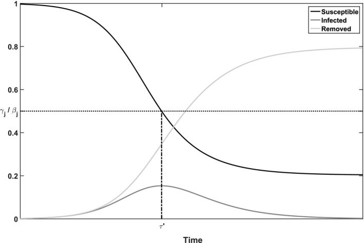
Illustration of the Deterministic SIR Model for Population j with Parameters γ _j = 1.5, β _j = 3, i ₀ = 10⁻⁶

Figure 2.

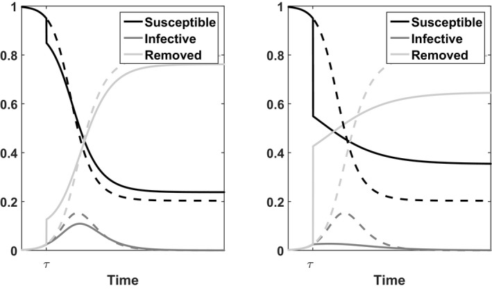
Illustration of the Deterministic SIR Model for Population j with Parameters γ _j = 1.5, β _j = 3, i ₀ = 10⁻⁶

Notes: Dashed lines represent the time course without vaccination. The solid lines represent the time course when either a fraction f _j = 0.1 (left panel) or f _j = 0.4 (right panel) is vaccinated at time τ when s _j(τ) = 0.95.

3.2. Vaccination

Vaccination reduces the fraction of susceptible individuals, in order to avoid or reduce an increase in the fraction of infected individuals. To formally define vaccination, we introduce the following notation. Let τ denote the time at which a fraction f _j of population j is vaccinated, with 0 ≤ f _j ≤ s _j(τ). Just prior to vaccination the system is in state (s _j(τ), i _j(τ)). Assume that the used vaccine is completely effective after a single dose and that vaccination takes no time, meaning that vaccination results in complete immunity immediately. Assume also that it is possible to identify the susceptible people. We refer to section 6 for a discussion of these assumptions. Under our assumptions vaccination causes a shift at time τ from state (s _j(τ), i _j(τ)) to state (s _j(τ) − f _j, i _j(τ)). This implies that r _j(τ) shifts to r _j(τ) + f _j. Figure 2 illustrates the changes at time τ.

To evaluate different vaccine allocations we base ourselves on the state of the system when t → ∞. This state is also referred to as disease‐free equilibrium, because ${lim}_{t\to \infty }{i}_j(t)=0$. We define G _j(f _j) as the final fraction of people susceptible in population j after vaccinating a fraction f _j of the susceptible people at time τ. More precisely, for $f_j\in [0,s_j(\mathit{\tau })]$

$$G_j(f_j)=\underset{t\to \infty }{lim}{s}_j(t),$$ (2)

with s _j(t) evolving according to Equations (1) for t > τ. The final fraction of people susceptible is closely related to the following concepts that we define here explicitly for future use:

• 1 Herd immunity: the protection of susceptible individuals against infection because they are surrounded by a sufficient number of immune individuals. The immunity from the latter group may result either from vaccination or from recovery from infection (cf. Fine 1993).
• 2 Herd effect: the proportion of all people that is spared from infection because of herd immunity, that is, the proportion of all people that is still susceptible when the epidemic has died out.

Thus G _j(f _j) measures the herd effect in population j. Section 4 studies G _j(f _j) in more detail using an alternative formulation of the function (see Appendix S1).

3.3. The Vaccine Allocation Problem

We are interested in allocating a limited amount of vaccines V in order to maximize health benefit, defined as the total number of people that escape infection:

$$\begin{array}{cc}\hfill max& \stackrel{\mathrm{herd}\mathrm{effect}}{\overbrace{\sum _{j\in J}{N}_j{G}_j(f_j)}}+\stackrel{\mathrm{direct}\mathrm{effect}}{\overbrace{\sum _{j\in J}{N}_j{f}_j}}\hfill \\ \hfill \text{s.t.}& \sum _{j\in J}{N}_j{f}_j\le V\hfill \\ & 0\le f_j\le s_j(\mathit{\tau })\forall j\in J\hfill \end{array}$$ (3)

Here, N _j denotes the size of population j. The objective function reflects that there are two ways to escape infection: either you are vaccinated (direct effect) or you escape infection without being vaccinated (indirect effect). Note that the fraction of people escaping infection without being vaccinated in population j is precisely the final fraction of susceptible people, that is, the herd effect G _j(f _j) introduced in section 3.2.

We discuss two equivalent formulations of the above allocation problem, using different objective functions in order to demonstrate the relation of our work to epidemiological literature. Firstly, in Theorem D1 we prove that it is optimal to always use the complete vaccine stockpile, that is, constraint ${\sum }_{j\in J}{N}_j{f}_j\le V$ will always be met with equality. This implies that the objective could be changed from maximizing the total effect of vaccination to maximizing only the herd effect. Secondly, maximizing the total effect of vaccination is equivalent to minimizing the final size of the epidemic, that is, the total number of people that get infected. The final size of the epidemic may be expressed as Z _j(f _j) = s _j(0) + i _j(0) − f _j − G _j(f _j) and Problem (3) is thus formally equivalent to a minimization problem involving this final size (e.g., Keeling and Shattock 2012, Wu et al. 2007). The relation between Z _j(f _j), f _j, and G _j(f _j) is illustrated in Figure 3. Note that the fraction G _j(f _j) may in fact increase for smaller values of f _j.

Figure 3.

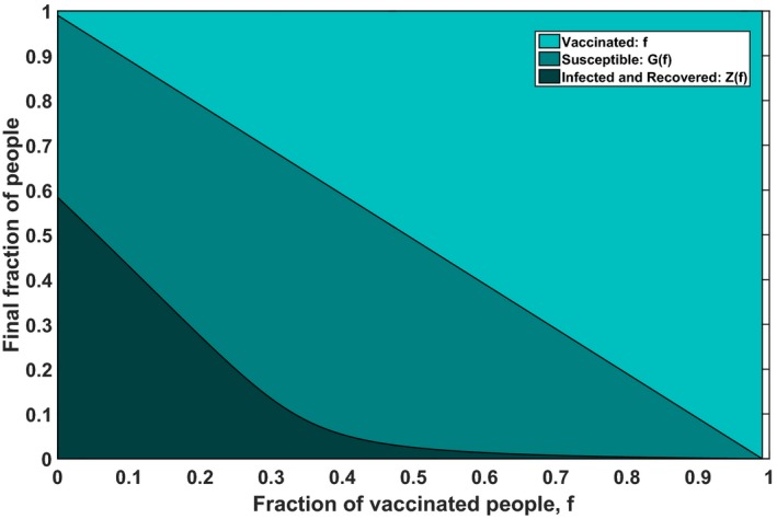
The Final State of the Epidemic for Different Vaccination Fractions, for an Epidemic with Basic Reproduction Ratio σ = 2 with (s ₀, i ₀) = (0.99, 0.01) and τ = 0 [Color figure can be viewed at http://wileyonlinelibrary.com]

4. Analysis of the Herd Effect

In order to study the allocation problem (3), section 4.1 analyzes and interprets the structure of the herd effect G(f) (we drop the subscript j for convenience). Based on this analysis we present our dose‐optimal vaccination fraction for a population in section 4.2 and compare this fraction to the so‐called critical vaccination fraction from literature in section 4.3. We extend our analysis to more general compartmental models in section 4.4. A minor detail is sorted out in section 4.5: we formally confirm that it is optimal to vaccinate as early as possible.

Figure 4 summarizes the main findings of this section and illustrates the structure of G(f). In sections 4.1 and 4.2 these results are derived formally.

Figure 4.

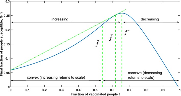
Illustration of the Structure of G(f), Which is Proven in Section 4: Theorems 1 and 2 Establish the Increasing–Decreasing and Convex–Concave Structure of G(f), Which is Illustrated in This Figure Using the Parameters (s ₀, i ₀) = (0.99, 0.01), σ = 3 and τ = 0 [Color figure can be viewed at http://wileyonlinelibrary.com]

Notes: Dashed lines represent the important vaccination fractions $\overline{f}$ (left), $f^{*}$ (right) and our dose‐optimal vaccination fraction $\tilde{f}$ (middle). The latter follows from Corollary 1. The straight dotted line illustrates that $\tilde{f}$ is the only non‐zero vaccination fraction for which the tangent line contains the point (0, G(0)).

4.1. Analysis of the Structure of the Herd Effect

In this and the next section, we present the main technical contribution of this study: a structural analysis of the herd effect G(f). Let $\mathit{\sigma }:=\frac{\mathit{\beta }}{\mathit{\gamma }}$. The overall structure of G(f) is established in the following theorems:

Theorem 1

There is a unique vaccination fraction $f^{*}=max(s(\mathit{\tau })-\frac{1}{\mathit{\sigma }},0)$ that maximizes the herd effect: the herd effect G(f) is increasing in f for all f < $f^{*}$, maximized for f = $f^{*}$ and decreasing for f > $f^{*}$.

Theorem 2

There exists a unique vaccination fraction $\overline{f}$ with $0\le \overline{f}\le f^{*}$ such that G(f) is strictly convex (G′′(f) > 0) for all $f<\overline{f}$ and strictly concave (G′′(f) < 0) for all $f>\overline{f}$.

We first briefly discuss how these results are derived. The proofs for these results and the supporting lemmas can be found in Appendix S2. We had to overcome a number of significant challenges, particularly because no explicit formulation of the herd effect G(f) exists. We develop an implicit relation characterizing G(f), and our proof departs from that relation. We note that despite almost 90 years of research on the SIR model, the convex‐concave shape and its repercussions for vaccine allocation have not been considered.

We next discuss the intuition behind these theorems, and the consequences that these results have for practice. The peak in the infections, illustrated in Figure 2, plays a critical role in determining the herd effect. At this peak, the proportion of susceptibles is equal to γ/β = 1/σ and so infections decrease for s(t) < 1/σ. Note that vaccinating with the fraction $f^{*}$ = s(τ) − 1/σ exactly results a proportion of susceptibles equal to 1/σ directly after vaccination, which leads to the following definition (cf., Keeling and Shattock 2012, Plans‐Rubió 2012):

• 1 Critical vaccination coverage: the smallest vaccination fraction that results in a decrease of infections directly after vaccination, denoted by $f^{*}$ as in Theorem 1.

Vaccination beyond $f^{*}$ thus protects individuals that would not be likely to contract the disease anyhow and expanding coverage beyond $f^{*}$ actually reduces the herd effect.

The primary effect of vaccination is that it reduces the number of people to be infected until the peak of infected is reached at s(t) = 1/σ. The convex‐concave structure results because this primary effect interacts with a secondary effect: f affects the specific time at which the peak occurs. This secondary effect is non‐monotonic, because it consists of two competing phenomena: (i) Vaccination lowers s(τ), thus reducing the further reduction in susceptibles needed until s(t) reaches 1/σ and (ii) Vaccination reduces the rate of initial exponential growth of infected people, thus inhibiting the speed of reduction of s(t). For small f the second effect dominates, resulting in a delayed peak as can be seen in Figure 2. For larger vaccination fractions, when s(τ) comes close to 1/σ, the first effect dominates rendering the peak to be advanced. A delayed peak is beneficial, since more time allows for more recoveries and consequently results in fewer infections at the peak. Small vaccination fractions benefit from the delayed peak, in addition to the primary effect, which results in the convex and increasing herd effect. For larger vaccination fractions the secondary benefit is reversed, which explains the concave increase.

The structure of the herd effect has some interesting practical consequences. Consider for example a policy maker that faces a pandemic influenza outbreak where the vaccine stockpile should be allocated over multiple populations with a comparable pre‐peak state. It is better to concentrate on one or few of these populations instead of allocating equally over all. By restricting attention to a few populations both the primary effect and the secondary effect can be fully exploited for a few populations resulting in a higher overall herd effect. Our results thus yield understanding why equitable allocations are often not efficient. This increased understanding is a contribution to the ethical debate on vaccine allocation.

Note that Theorem 2 does not rule out that $\overline{f}=0$, in which case there is no convex part of G(f). Similarly, by Theorem 1 we may have $f^{*}$ = 0, in which case G(f) is never increasing. The following theorem investigates these issues. It features the constant C that is defined as C = 2/σ + W[−σ exp {−σ(s ₀ + i ₀) +  log (s ₀)}]/σ, where W[·] is the Lambert W function and C > 1/σ (cf. Appendix S5).

Theorem 3

For the structure of G(f) we can distinguish three cases based on s(τ), the proportion of susceptibles at the moment of vaccination τ:

1. C < s(τ) < 1: We have $f^{*}>\overline{f}>0$. Thus G(f) is increasing and convex between 0 and $\overline{f}$, increasing and concave between $\overline{f}$ and $f^{*}$, and decreasing and concave above $f^{*}$.

2. 1/σ < s(τ) ≤ C: We have $f^{*}$ > 0 and $\overline{f}=0$. Thus G(f) is increasing and concave between 0 and $f^{*}$, and decreasing and concave above $f^{*}$.

3. 0 ≤ s(τ) < 1/σ: We have $\overline{f}=f^{*}=0$. Thus G(f) is decreasing and concave everywhere.

Figure 4 graphically illustrates the herd effect G(f) with parameters for which C = 0.7092. Since we use s(τ) = s ₀ = 0.99, the figure shows the most general shape (i). Theorem 3 follows from the intuitive discussion earlier in this section. For s(τ) high enough (more precisely higher than C) the peak in infections can be delayed with small vaccination fractions, resulting in the convex increase in the herd effect. When s(τ) is below C the peak can not be delayed through vaccination and the herd effect has no convex part. If s(τ) < 1/σ, the population is already in a post‐peak state with infections declining. This implies that the risk of getting infected for the people who are still susceptible is relatively low. In that case $f^{*}$ = 0 and vaccination reduces the herd effect, because you vaccinate people that were unlikely to get infected in the first place.

Thus, policy makers that face an outbreak of pandemic influenza for example, should resist the pressure to vaccinate in areas with many infected people. Indeed, when infections are close to the peak, the effect of vaccination is lower. Vaccinating in post‐peak areas is even less effective, because the people that you vaccinate were not likely to become infected anyhow (cf., Teytelman and Larson 2013). Thus, it is best to vaccinate in pre‐peak areas where s(τ) >> 1/σ. But to achieve most in such populations, concentration of effort is needed. In sections 4.2 and 5.1 we will discuss this in more detail.

4.2. The Dose‐Optimal Vaccination Fraction

In this section, we present a third important vaccination fraction, next to the vaccination fractions $f^{*}$ and $\overline{f}$ defined in Theorems 1 and 2. To explore the impact of vaccination we should take into account that susceptible people will escape infection even without vaccination. Accordingly, we define:

• Additional herd effect:the herd effect achieved through vaccination minus the herd effect that would already be present without vaccination; denoted by G(f) − G(0).

We introduce the function D(f) to measure the average additional herd effect per dose of vaccine:

$$D(f)=\frac{1}{f}[G(f)-G(0)]$$ (4)

Note that D(f) can also be interpreted as the average slope of the herd effect G(f) on the interval [0, f]. We derive following result:

Corollary 1

The function D(f) as defined by Equation (4) is maximized by the unique vaccination fraction $\tilde{f}$ for which $G^{\prime }(\tilde{f})=D(\tilde{f})$. The function D(f) is increasing for $f<\tilde{f}$ and decreasing for $f>\tilde{f}$.

We have thus determined three important vaccination fractions of which the relation is presented in the following lemma:

Lemma 1

Consider the following three vaccination fractions: $f^{*}$ as defined in Theorem 1, $\overline{f}$ as defined in Theorem 2 and $\tilde{f}$ as defined in Corollary 1. The following relation holds: $\overline{f}\le \tilde{f}\le f^{*}.$

Corollary 1 and Lemma 1 are illustrated in Figure 5. Observe that at $\tilde{f}$ the line connecting G(0) and $G(\tilde{f})$ is also the tangent line at $G(\tilde{f})$. Because of the convex‐concave structure of the herd effect G(f) there is only a single vaccination fraction $\tilde{f}$ for which this holds, and this fraction must lie between $\overline{f}$ and $f^{*}$. The interpretation of Corollary 1 is that $\tilde{f}$ gives the highest additional herd effect per dose of vaccine, which leads to the following definition:

Figure 5.

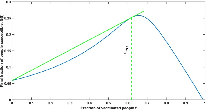
Illustration of the Dose‐Optimal Vaccination Fraction $\tilde{f}$ Using the Parameters (s ₀, i ₀) = (0.99, 0.01), σ = 3, and τ = 0 [Color figure can be viewed at http://wileyonlinelibrary.com]

Notes: The slope of the straight line represent the value of D(f) for $\tilde{f}$. Observe that any other line starting at G(0) and intersecting with G(f) would be less steep and not tangent to G(f).

• 1 Dose‐optimal vaccination fraction: the vaccination fraction that maximizes the average additional herd effect per dose of vaccine in a population, denoted by $\tilde{f}$.

A discussion of the implications of Corollary 1, and a comparison of the dose‐optimal $\tilde{f}$ with the critical vaccination coverage $f^{*}$ are provided in the next section.

4.3. Dose‐Optimal and Critical Vaccination Coverage

Our dose‐optimal vaccination fraction $\tilde{f}$ and the vaccination fraction $f^{*}$ represent two different concepts in vaccine allocation. We compare the dose‐optimal vaccination fraction $\tilde{f}$ with the critical vaccination coverage $f^{*}$ and illustrate these fractions for different values of σ in Table 2. The table shows that $\tilde{f}$ and $f^{*}$ are indeed quite different. For σ growing large, both $\tilde{f}$ and $f^{*}$ converge to s(τ) (cf., Lemma B4 in Appendix S2.3), but this limit is not very interesting because σ is between 2 and 20 for most diseases. For example, σ ≈ 3 for influenza, σ ≈ 3.5–6 for smallpox, σ ≈ 6–7 for rubella and σ ≈ 16–18 for measles (Keeling and Rohani 2008).

Table 2.

Illustration of the Three Important Vaccination Fractions $\overline{f}$, $\tilde{f}$, and $f^{*}$ for Increasing σ

σ	2	3	5	10	15	20	25	30	50	100
$\overline{f}$	0.3376	0.5411	0.7086	0.8398	0.8857	0.9094	0.9240	0.9340	0.9546	0.9712
$\tilde{f}$	0.4134	0.6193	0.7746	0.8855	0.9211	0.9386	0.9490	0.9560	0.9697	0.9799
$f^{*}$	0.4900	0.6567	0.7900	0.8900	0.9233	0.9400	0.9500	0.9567	0.9700	0.9800

To calculate the numbers an initial state (s ₀, i ₀) = (0.99, 0.01) and s(τ) = 0.99 is used.

This article is being made freely available through PubMed Central as part of the COVID-19 public health emergency response. It can be used for unrestricted research re-use and analysis in any form or by any means with acknowledgement of the original source, for the duration of the public health emergency.

As discussed in section 4.2 the vaccination fraction $\tilde{f}$ results in the most efficient allocation per dose of vaccine in a population. The vaccination fraction $f^{*}$ on the other hand is attractive from another perspective and has been advocated in literature (e.g., Keeling and Shattock 2012, Plans‐Rubió 2012). It does not only maximize the herd effect, but also directly results in a decrease in infected individuals at time τ.

Corollary 1 and Lemma 1 clearly show that $\tilde{f}$ makes more efficient use of vaccines then $f^{*}$. This can be intuitively understood as follows. Note that $f^{*}>\tilde{f}$. Our intuitive interpretation of Theorem 2 reveals that while vaccination initially delays the timing of the peak of infected, vaccinating with higher vaccination fractions will actually render the peak to be advanced. As a consequence, vaccines issued to expand coverage from $\tilde{f}$ to $f^{*}$ in a population are used inefficiently. We give an example using the settings of Table 2 and σ = 3. In that case, the vaccines between 0 and $\tilde{f}$ result in an average herd effect of 0.31 per dose, whereas this average is only 0.17 per dose for the vaccines between $\tilde{f}$ and $f^{*}$. Hence, vaccinating beyond $\tilde{f}$ to achieve $f^{*}$ is costly, and not a good use of a limited vaccine stockpile.

In literature optimal vaccination has often been explained in terms of avoiding the further increase in infected individuals, which relates to vaccinating with $f^{*}$ (cf., Keeling and Shattock 2012, Wu et al. 2007, Yuan et al. 2015). Avoiding an increase of infected people is suitable when there are initially no infected individuals, that is, for “pre‐pandemic vaccination” (the limit i ₀ ↓ 0). However, allocating a limited vaccine stockpile typically goes hand in hand with a sudden outbreak: the limited stockpile arises because not enough time is available to produce more. This arguably renders pre‐pandemic vaccination unrealistic in combination with allocating a limited vaccine stockpile. In the case of influenza, this implies that the assumption of a limited stockpile is more realistic for pandemic influenza than for seasonal influenza. Extant literature has focused mainly on the less realistic case of a limited stockpile and pre‐pandemic vaccination, for which $f^{*}$ and $\tilde{f}$ coincide numerically as we show in Appendix S2.3, and has thus missed the conceptual distinction between critical and dose‐optimal vaccination. In general the concepts of dose‐optimal vaccine allocation and avoiding an increase in infections are substantially different. The explanation of literature is therefore not generalizable.

4.4. The SEIR Model and Other Extensions

An important extension of the standard SIR compartmental model is the SI ⁿ R model with n different consecutive infectious stages. This extension allows to include a latent period or multiple levels of infectivity. Let β _k and γ _k denote respectively the transmission rate and recovery rate in infectious stage k. A special case of the SI ⁿ R model for which n = 2 is the SEIR model. Compared to the SIR model the SEIR model has an additional compartment E containing the individuals that are exposed and hence infected, but not yet infectious. We derive our results for the general SI ⁿ R model, in which there are arbitrary many additional compartments:

Lemma 2

The results of Theorem 1, Theorem 2, Theorem 3 and Corollary 1 also apply to the SI ⁿ R model with $\mathit{\sigma }={\sum }_{k=1}^n\frac{{\mathit{\beta }}_k}{{\mathit{\gamma }}_k}$. In particular, for each SI ⁿ R model with given initial conditions there exist vaccination fractions $\overline{f}$, $\tilde{f}$ and $f^{*}$ that together characterize the convex–concave and increasing–decreasing shape of the herd effect.

Theorem 1, Theorem 2, Theorem 3 and Corollary 1 form the basis for the analysis of the vaccine allocation problem in section 5. By Corollary 2 the results derived in section 5 are valid for the more general SI ⁿ R model. The interested reader is referred to Appendix S3, where we formally analyze the SI ⁿ R model.

4.5. The Optimal Timing of Vaccination

We sort out a minor detail by formally proving that vaccination should ideally be carried out as soon as possible. Thereto we determine the time τ at which the total effect of vaccination, that is, G(f, s(τ)) + f, is maximized. Assume that we have a fixed vaccine stockpile, V, such that a fraction of the population can be vaccinated is restricted by $\frac{V}{N}$, where N is the population size. If s(τ) ≤ V/N, all susceptible people can be vaccinated and the objective function for f = s(τ) reduces to s(τ), because  lim_f↑s(τ) G(f) = 0 by Theorem B1. If s(τ) > V/N, all available doses of vaccine are used and $f=\frac{V}{N}$. In Lemma B.6 we derive that the herd effect G(f, s(τ)) is increasing in s(τ) in that case. Therefore, to maximize the number of people that escape infection one should vaccinate as soon as possible in an ideal world. A policy maker that has to allocate a limited vaccine stockpile over a number of populations that face an outbreak of pandemic influenza should therefore concentrate on the population in which the outbreak has least progressed.

5. Analysis of the Vaccine Allocation Problem

In this section, we analyze the vaccine allocation problem (3), using the characterization of the objective function in Theorems 1, 2, and 3. These theorems establish that our vaccine allocation problem is a combinatorial optimization problem that is likely difficult to solve to optimality (cf., Srivastava and Bullo 2014). However, in this section we show that there is an interesting structure in the optimal solution. Section 5.1 presents this central insight. Section 5.2 considers an interesting special case to gain more understanding of the structure of the solution. Section 5.3 translates the results gained in sections 5.1 and 5.2 into insights and simple guidelines for arriving at an efficient allocation. In section 5.4, we illustrate how the insights from the non‐interactive case can be applied to geographically distant populations that interact with each other.

5.1. The Optimal Allocation

We characterize the optimal allocation, which is the solution to Problem (3). We will make a few non‐restrictive assumptions to allow us to focus on the most interesting cases. Firstly, we assume that V < $V^{*}$, where $V^{*}={\sum }_{j\in J}{N}_j{f}_j^{*}$, reflecting our focus on severe shortages of vaccines. As argued in section 4.3, this is a realistic assumption in case of a sudden outbreak such as pandemic influenza. Indeed, with V ≥ $V^{*}$ all locations can reach critical vaccination coverage $f_j^{*}$, stopping any further increase of infections. Moreover, we observed in section 4.1 that post‐peak populations (with s _j(τ) < 1/σ _j) should not receive vaccination until all pre‐peak populations receive at least $f_j^{*}$. Thus, here we assume that all populations are pre‐peak (s _j(τ) > 1/σ _j). We refer to Appendix S4 for a description of the optimal allocation in case these assumptions are relaxed.

We will show that every optimal solution to problem (3) is linked to a certain marginal efficiency ω:

• 1 Marginal efficiency: the increase in herd effect if one additional dose of vaccine would be allocated to a population, calculated as the derivative of G _j(f _j) with respect to f _j.

Populations j ∈ J are vaccinated with marginal efficiency ω if $G_j^{\prime }(f_j)=\mathit{\omega }$. In the optimal solution, by KKT conditions every population that is partially vaccinated must be vaccinated with marginal efficiency ω. However, potentially two vaccination fractions f _j may satisfy $G_j^{\prime }(f_j)=\mathit{\omega }$:

• 1 Regular fraction: the vaccination fraction f _j that results in a marginal efficiency ω and lies in the domain where the herd effect is concave, that is, $f_j>{\overline{f}}_j$.
• 2 Exceptional fraction: the vaccination fraction f _j that results in a marginal efficiency ω and lies in the domain where the herd effect is convex, that is, $f_j<{\overline{f}}_j$.

In the optimal solution, there are three possible vaccination fractions for every population j ∈ J: (i) the regular fraction, (ii) the exceptional fraction or (iii) f _j = 0 and population j is not vaccinated at all. Figure 6 illustrates these three possibilities for population j.

Figure 6.

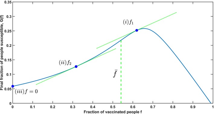
Illustration of the Structure of the Optimal Allocation, Using the Parameters (s ₀, i ₀) = (0.99, 0.01), σ = 3, and τ = 0 [Color figure can be viewed at http://wileyonlinelibrary.com]

Theorem 4

(Central Insight) Every optimal solution to Equation (3) can be characterized as follows:

1. A subset of populations J′ ⊆ J is vaccinated with the regular fraction that corresponds to marginal efficiency ω.

2. Possibly another population k is also vaccinated with marginal efficiency ω, but with the exceptional fraction for which $f_k<\overline{f_k}$.

3. The remaining populations are not vaccinated at all.

Determining ω for a specific problem is difficult, which relates back to the combinatorial nature of Problem 3. Still, a key insight can be derived from Theorem 4: A policy maker should focus on a subset of populations when allocating vaccines and leave other populations unvaccinated. By doing so the benefits of the herd effect are best exploited, because only a concentrated effort can fully harness both the primary and the secondary effects of vaccination. The structure of the optimal allocation thus clearly brings about complex decisions for policy makers, who also have to take equity considerations into account. Our results show that mathematically optimal allocations are inherently inequitable due to the nonlinear dynamics of epidemics. Hence, policy makers are to some extend forced to choose between equity and efficiency. For a further discussions of the ethical dimension of vaccine allocation we refer to section 7.

5.2. The Special Case: Identical Parameters

We illustrate the intuition behind the central insight for an interesting special case: the case of populations having identical disease parameters. This special case implies identical functions G _j(f _j) := G(f _j) for all j ∈ J (σ _j := σ, $s_0^j:=s_0$, $i_0^j:=i_0$ for all j ∈ J). In that case the regular fraction f _j for a certain marginal efficiency ω is the same for all populations j. This implies that the allocation described in (i) of Theorem 4 is a pro rata allocation over the subset J′, with pro rata as usual denoting an allocation in which the doses of vaccine are distributed equally with respect to population size, such that the vaccination fraction is the same in all selected populations. For this special case the optimal allocation may be characterized in more detail.

Based on the results derived in section 4, we conclude that our optimization problem is a knapsack problem with convex‐concave return functions. Ginsberg (1974) study an investment problem over multiple factories with convex‐concave production functions. Mathematically, this problem is equivalent to our vaccine allocation problem for the special case G _j(0) = 0 and N _j = N for all j ∈ J. Intuitively, this special case corresponds to a situation with a shifted herd effect and all sub‐populations having the same size. We build upon the results of Ginsberg (1974) to characterize the optimal vaccine allocation in the following theorem.

Theorem 5

Consider a set of populations J with ∀j: G _j(f) = G(f) and a total available amount of resources equal to V. Let |J| = n and order the populations such that N ₁ ≤ ⋯ ≤ N _n. The optimal allocation for particular cases is as follows:

1. if $V<\tilde{f}{N}_1$, then allocate only to the smallest population. Set f ₁ = V/N ₁ and f _j = 0 for j = 2, …, n.

2. if $V={\sum }_{j\in K}\tilde{f}{N}_j$ for a subset K ⊆ J, then set $f_j=\tilde{f}$ for j ∈ K and f _j = 0 for j ∉ K.

3. if $V>{\sum }_{j\in J}\tilde{f}{N}_j$, then allocate pro rata over all the populations: $f_j=\frac{V}{{\sum }_{j\in J}{N}_j}$ for all j ∈ J.

The proof of this theorem can be found in Appendix S4. Theorem 5 shows that in order to make the best possible use of the herd effect, decision makers should try to vaccinate close to $\tilde{f}$ in (a subset of) the populations. They should allocate all vaccines to the smallest population if the vaccination fraction $\tilde{f}$ cannot be attained in any of the populations (case (a)). For very large vaccine stockpiles, policy makers do best in selecting the pro rata allocation over all populations (case (c)). Note that Theorem 5 only specifies the allocation in specific cases of vaccine stockpiles, but can be extended to any available amount of vaccines. However, the description of the optimal allocation for a general vaccine stockpile is quite technical and less insightful and is therefore omitted. In general, the optimal allocation changes continuously for small changes in V. For larger changes discontinuities may arise when jumping from one subset K to the other in item (b) of Theorem 5.

5.3. Discussion of the General Case—The Switching Behavior

The vaccine allocation problem that we study is NP‐hard, but we have derived an interesting structure in Theorem 4 and section 5.2. In this section we translate this structure to insights and a simple guideline for arriving at an efficient allocation.

Recall that in the special case discussed in section 5.2 a decision maker should look for a subset of populations such that it is feasible to vaccinate these populations close to the fraction $\tilde{f}$ that yield the highest additional herd effect per allocated dose. In the general case the parameters may differ per population, causing the functions G _j(·) to be different for different populations j. This implies that there is no longer a single value for $\tilde{f}$, but an ${\tilde{f}}_j$ for every population j ∈ J. The additional herd effect per dose of vaccine in population j is the highest at ${\tilde{f}}_j$ and decreases as the vaccination fraction moves away from ${\tilde{f}}_j$ in either direction. This has the following implications for the optimal allocation: a decision maker should select a subset of populations and divide the vaccines over them such that these populations are vaccinated with a fraction close to their dose‐optimal fractions ${\tilde{f}}_j$. The marginal efficiency ω of Theorem 4 determines how close the vaccination fraction exactly is to the dose‐optimal fraction. In any case, Theorem 4 guarantees that the vaccination fraction lies in the interval $[{\overline{f}}_j,f_j^{*}]$ for the populations in the selected subset, except for at most one population which can be vaccinated with a fraction below $\overline{f_j}$.

The recommendation given by Wu et al. (2007), Keeling and Shattock (2012), Yuan et al. (2015) to maximize the herd effect in some populations by setting $f_j=f_j^{*}$ is thus incorrect in typical practical settings of a limited vaccine stockpile, e.g., during an outbreak of pandemic influenza. A decision maker should vaccinate close to ${\tilde{f}}_j$ to use the vaccines efficiently in every population; any additional vaccinations used to reach critical coverage $f^{*}$ in j are ineffective as discussed in section 4.3.

Using the above characterization of the optimal allocation we can also explain the switching behavior. The smallest populations are prioritized for small vaccine stockpiles, as the number of doses of vaccine required to reach ${\tilde{f}}_j$ is smaller in those populations. When the stockpile size increases, we can vaccinate close to the dose‐optimal vaccination fraction in larger populations and hence priority shifts to these populations. Numerical analysis of the optimal vaccine allocation (e.g., by Keeling and Shattock 2012) shows switch points where a small increase in vaccine stockpile results in a completely different allocation. Our analysis explains these switch points: they are related to a change in the subset of populations to approach the dose‐optimal vaccination fraction.

The structure of the optimal allocation is illustrated in Figure 7, where we use the example from the introduction with three populations of size N ₁ = 10,000, N ₂ = 20,000 and N ₃ = 40,000 respectively. The following parameters are used: τ = 0, σ _j = 2 for j = 1,2,3 and initial states $(s_0^1,i_0^1)=(0.985,0.015),(s_0^2,i_0^2)=(0.988,0.012)$ and $(s_0^3,i_0^3)=(0.990,0.010)$. In Figure 7 we indeed observe that the vaccinated populations receive a number of allocated vaccines that is close to ${\tilde{V}}_j$.

Figure 7.

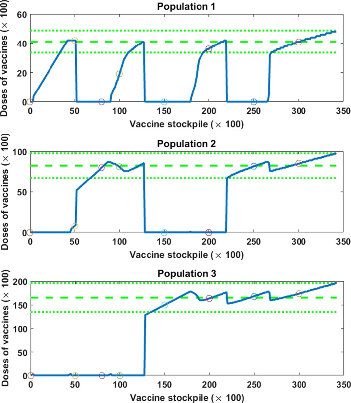
The Graphs Present the Optimal Vaccine Allocation (the solid lines) over Three Populations for Different Sizes of Vaccine Stockpile [Color figure can be viewed at http://wileyonlinelibrary.com]

Notes: The dashed and dotted lines indicate the important vaccination fractions: the dashed line in the middle equals ${\tilde{V}}_j={\tilde{f}}_j{N}_j$, the upper dotted line equals $V_j^{*}=f_j^{*}{N}_j$ and the lower dotted line equals ${\overline{V}}_j={\overline{f}}_j{N}_j$. The circles indicate the values from Table 1.

To relate Figure 7 to the description of the optimal allocation in Theorem 4, we explain the optimal allocation for two vaccine stockpile sizes: V = 5000 and V = 10,000. For V = 5000, the optimal strategy is roughly to allocate 4200 vaccines to population 1 and the remaining 800 to population 2. We thus see all three vaccination possibilities of Theorem 1 present: (i) population 1 gets the regular fraction, (ii) population 2 the exceptional fraction and (iii) population 3 is not vaccinated at all. For V = 10,000, we see the roles of population 1 and 2 reversed with population 1 getting 1900 vaccines and population 2 receiving the remaining 8100. We can calculate that ${\tilde{V}}_1={\tilde{f}}_1{N}_1=3963$, ${\tilde{V}}_2={\tilde{f}}_2{N}_2=8173$ and ${\tilde{V}}_3={\tilde{f}}_3{N}_3=$16,702. The two examples for V, as well as the optimal allocations in Table 1 and Figure 7, illustrate that vaccines in the optimal allocation are allocated such that the vaccination fractions in the vaccinated populations are always close to the dose‐optimal fraction and that at most one population has a substantial lower vaccination fraction.

We use our explanation of the optimal allocation in terms of the dose‐optimal vaccination fraction to derive a guideline for the vaccine allocation problem (3). This simple heuristic does not find the optimal solution, but it does capture an important structure of the optimal solution: as many populations as possible are vaccinated with their dose‐optimal vaccination fraction ${\tilde{f}}_j$.

1. We order populations based on the benefits per dose of vaccine such that $D_1({\tilde{f}}_1)\ge \cdots \ge D_n({\tilde{f}}_n)$, where the function D(f) is defined in Equation (4).

2. Following the order of step 1, we vaccinate as many populations as possible with their dose‐optimal vaccination fraction until the vaccine stockpile is insufficient to reach dose‐optimal coverage for the next population (case 1) or until dose‐optimal coverage is reached for all populations (case 2).

3. We allocate the remaining vaccines. In case 1, these vaccines are allocated to the unvaccinated population in which these vaccines are most beneficial (i.e., the population for which allocating the remaining vaccines would result in the highest D _j(f _j)). In case 2, we allocate the remaining vaccines pro rata over all populations.

We evaluate the performance of the heuristic as well as the gains of using the optimal allocation and compare to the equitable allocation in Table 3. We note that only a stockpile size of 30,000 is sufficient to achieve dose‐optimal coverage in all three populations. Since the direct effect of vaccination is not affected by the allocation, we focus only on the herd effect. In particular, we look at the additional herd effect which leaves out the herd effect that is already achieved without any vaccination:

$$\text{additional herd effect}=\sum _{j\in J}{N}_j(G_j(f_j)-G_j(0))$$ (5)

The table shows that the optimal allocation is significantly more effective in harnessing the herd effect than the pro rata allocation. We also observe that the allocation heuristic performs close to optimal. It captures the same structure as the optimal solution, which results in a good performance.

Table 3.

The Additional Herd Effect (5) for Three Different Allocation Strategies for Various Vaccine Stockpiles

Vaccine stockpile	Equitable allocation	Heuristic allocation	Optimal allocation	Relative improvement optimal over equitable allocation (%)
2000	671	762	762	+13.56
5000	1742	2037	2037	+16.93
8000	2893	3235	3511	+21.36
10,000	3707	4274	4274	+15.30
15,000	5912	6265	6702	+13.36
20,000	8350	8842	8910	+6.71
25,000	10,930	11,032	11,170	+2.20
30,000	13,255	13,226	13,264	+0.07

The equitable allocation allocates pro rata over all populations, the heuristic allocation is determined via the heuristic described in section 5.3 and the optimal allocation is specified in Table 1 and Figure 7. The population sizes are: N ₁ = 10,000, N ₂ = 20,000 and N ₃ = 40,000.

This article is being made freely available through PubMed Central as part of the COVID-19 public health emergency response. It can be used for unrestricted research re-use and analysis in any form or by any means with acknowledgement of the original source, for the duration of the public health emergency.

To investigate the impact of heterogeneous σ we have performed an additional experiment in which the disease parameters of the populations change to σ ₁ = 1.5, σ ₂ = 2, σ ₃ = 2.5. The relative improvement of the optimal allocation over the pro rata allocation increases from 0–21% to 5–72% in that case. We have also investigated an algorithm based on minimizing R ₀. However, the performance of this algorithm was poor and the corresponding results are therefore not reported.

5.4. Interaction

Our model can be applied to geographically distant populations, and one might wonder how our insights are affected when these populations exhibit some interaction in the form of mutual infections. From a theoretical perspective, our results continue to hold for sufficiently weak interactions, while they are invalidated by sufficiently strong interactions. Indeed, for strong interaction sub‐populations start to behave like a single large population, implying that pro rata allocation should perform well.

We determine at what level of interaction our results start to deteriorate by comparing the results derived for the non‐interacting case with the structure of the optimal allocation for various levels of interaction. The SIR model with interaction is given by the following differential equations (Diekmann et al. 2012):

$$\begin{array}{cc}\hfill \frac{d{s}_j}{dt}& =-\sum _{k\in J}{\mathit{\beta }}_{jk}{s}_j{i}_k\hfill \\ \hfill \frac{d{i}_j}{dt}& =\sum _{k\in J}{\mathit{\beta }}_{jk}{s}_j{i}_k-{\mathit{\gamma }}_j{i}_j\hfill \\ \hfill \frac{d{r}_j}{dt}& ={\mathit{\gamma }}_j{i}_j\hfill \end{array}$$ (6)

We consider an example with three populations with the population sizes and initial states being the same as in the non‐interacting example presented in section 5.3. We use the following parameters: γ _j = 1 and β _jj = β = 2 for all j ∈ J. The interaction is determined as follows: ${\mathit{\beta }}_{jk}=c\mathit{\beta }\frac{N_k}{{\sum }_{m\ne j}{N}_m}$ for j, k ∈ J and j ≠ k, such that ∑_k≠j β _jk = cβ for all j ∈ J, with c being the interaction factor: interaction between populations is a factor 1/c weaker than interaction within populations.

The vaccination fractions ${\overline{f}}_j$, ${\tilde{f}}_j$ and $f_j^{*}$ are computed by numerical evaluation of Equation (6) fixing f _k = 0 for k ≠ j. Perhaps surprisingly, we still observe the convex–concave relation between the herd effect and the used vaccination fraction in that population. Numerical experiments in which we determine the optimal allocation via enumeration show that the insights for the non‐interacting case carry over. Up to an interaction factor of 0.02 the switching pattern is still clearly visible up to vaccine stockpiles of around 30% of the total population size. For a factor 0.05 switching priorities occur only for relatively small stockpiles and for a factor 0.1 the optimal allocation does no longer display any switching behaviour. Yet for all compared levels of interaction (0.01, 0.02, 0.05, and 0.1) the optimal allocation of small vaccine stockpiles remains unequitable, prioritizing initially only one population. Numerical results also show that ignoring interaction performs close to optimal and even outperforms the equitable allocation. We refer to Appendix S6 for a graphical illustration of the numerical experiments mentioned in this section.

We assume that the interaction factor c is relatively small, which conforms to Wu et al. (2007) who note that individuals spend on average more than 97% of their time in their home regions. Also Sun et al. (2009) and Mamani et al. (2013) derive their results for sufficiently small between‐country transmission rates. In the latter paper this is specified as the assumption that β _ij β _jk ≈ 0. Our results indicate that vaccine allocation can benefit from increasing returns to scale also in case of larger interaction between populations. Hence, our structural results that characterize the optimal allocation apply for typical interacting models.

6. Discussion of Assumptions

We briefly discuss the effect of modeling assumptions, extensions and the generality of the results. Our results continue to hold when several assumptions are relaxed as will be discussed here. We assume that the vaccine is completely effective and results in immunity directly. The effectiveness of a vaccine can be incorporated with an efficacy parameter that rescales the vaccination fraction (cf. Hill and Longini Jr 2003, Mylius et al. 2008). A delay in immunity can be approximated by using a slightly lower value for s(τ) than at the vaccination moment. We also assume that it is possible to identify susceptible individuals. If this is not the case, some of the vaccines would be administered to infected or immune people. Under the condition that the vaccines are only effective for susceptible people, this implies that the proportion of people effectively vaccinated equals fs(τ). That is, we can simply rescale a parameter to account for situations where susceptible people cannot be identified. All these small adjustments in the parameters do not change the structure of the herd effect and the optimal vaccine allocation. Thus the structure described in the theorems and lemmas continues to hold. Finally, we assume that a single dose of vaccine is sufficient to achieve immunity. Our results cannot be directly applied to the situation where multiple doses of vaccine are given to an individual, particularly because there often needs to be a minimum time in between administering consecutive doses. As the epidemic continues to spread in the meantime, this brings extra complexity to the problem (cf., Duijzer et al. 2017a).

The results in this study are established under the assumption that vaccination is the only intervention used. However, in practice vaccination is often combined with hygiene measures and treatment or isolation of infected patients. These other interventions change the course of the epidemic by influencing for example the transmission rate or the recovery rate. Further research is needed to investigate how the results derived in this study carry over when multiple interventions are combined.

This study uses an analytical approach to determine the essential problem characteristics that govern the structure of the solution. This implies that the structure of the solution can be generalized to problems with the same characteristics. Note that the deterministic model considered in this study can be seen as the fluid approximation of a stochastic model. Unpublished numerical results by the authors indicate that the convex‐concave pattern in the herd effect also holds for this stochastic SIR model. This is an indication that the insights of this study carry over, although proving convexity is even more difficult for the stochastic model. For populations with interaction we numerically illustrate in section 5.4 and Appendix S6 that the insights gained from the non‐interacting case can still be applied, which is in line with the findings of Wu et al. (2007).

7. Conclusions

In this study, we analyze the optimal allocation of a vaccine stockpile in order to maximize the health benefit, where we define health benefit as the total number of people that escape infection. We find that vaccination can have a secondary effect in addition to the primary one, which causes a second dose of vaccine to have a bigger effect than the first. Based on this result we show that there is a unique vaccination fraction that results in the highest health benefit per dose of vaccine in a population and introduce the term dose‐optimal for this fraction.

We discuss the qualitative difference between dose‐optimal and critical vaccination coverage, where the latter aims at maximizing health benefits. We show that policy makers should stop vaccinating before the health benefits are maximized in order to achieve the most efficient allocation. The final doses needed to maximize health benefits in a population yield more in another population.

We characterize the solution of the vaccine allocation problem and we show the crucial importance of the dose‐optimal vaccination fraction. A single dose of vaccine may be a drop in the ocean, but multiple doses together can save a population. When vaccines are scarce, vaccine effort should be concentrated on a few populations to benefit from a high vaccine coverage. Policy makers should therefore select a subset of populations to which the vaccines are allocated. By focusing on a limited number of populations, the available vaccine stockpile is used more efficiently than by allocating pro rata over all populations.

In the distribution of vaccines many logistical aspects play a role, ranging from transporting the vaccines from a central warehouse to health facilities, to setting up points of dispensing where people can be vaccinated. Allocating vaccines only to certain populations, might be easier from an logistical viewpoint than allocating to all populations. On the other hand, if vaccines are stockpiled locally, redistributing vaccines might lead to coordination problems (cf., Mamani et al. 2013). Further research could study the logistical consequences of vaccine allocation.

Vaccine allocation has an ethical dimension, unlike many other resource allocation problems where equity does not play a role. In this study, we distinguish between groups of people based on geography. Others use age groups or risk groups (e.g., Goldstein et al. 2009, 2012, Medlock et al. 2009, Mylius et al. 2008). Although prioritizing based on geography might seem unfair, geography might play a role in outbreaks of influenza, measles or in bioterror attacks. In the past, there have been outbreaks with large regional differences such as the 2009 H1N1 pandemic (Centers for Disease Control and Prevention 2009b). In situations with a large asymmetry between the regions, a geographic assymetric approach is perhaps more easily accepted. However, our results also show that sometimes asymmetric choices should be made in symmetric cases (e.g., two regions with the same parameters and disease progression). In those situations, our optimal allocation is less politically viable, and new ideas are needed to reconcile equity and efficiency in such cases.

Thus, the policy that we describe as optimal need not be the best policy if we also take equity considerations into account. The CDC for example uses ethical guidelines in decision making on influenza pandemics (Kinlaw and Levine 2007). These ethical guidelines are the result of an ethical debate on finding good vaccine allocations. The results derived in this study can be a valuable contribution to this ethical debate. Our optimal allocations can be used as a benchmark to determine the effects on the final size of an epidemic if a suboptimal policy is selected motivated by fairness. Next to that, policy makers can use strategies in which they balance between efficiency and equity. For example, they can reserve part of the vaccine stockpile for pro rata allocation and allocate the remaining vaccines optimally (cf., Kaplan and Merson 2002, Wu et al. 2007). Another possibility is to add equity constraints that either set minimum levels for vaccination in each region or restrict the relative difference between populations (Teytelman and Larson 2013). Our relatively simple model, and the analytical results we obtained for it, could be a valuable starting point to test ideas on balancing equity, political viability, and effectiveness of vaccine allocations.

Supporting information

Appendix S1: The Herd Effect Function.

Appendix S2: Analysis of the Herd Effect—Lemmas and Theorems.

Appendix S3: Generality of the Function G(f).

Appendix S4: Optimal Vaccine Allocation—Theorems and Proofs.

Appendix S5: The Lambert W Function.

Appendix S6: Interacting Populations.

References

- Adida, E. , Dey D., Mamani H.. 2013. Operational issues and network effects in vaccine markets. Eur. J. Oper. Res. 231(2); 414–427. [DOI] [PMC free article] [PubMed] [Google Scholar]
- Ağrali, S. , Geunes J.. 2009. Solving knapsack problems with S‐curve return functions. Eur. J. Oper. Res. 193(2): 605–615. [Google Scholar]
- Arino, J. , Van den Driessche P.. 2003. A multi‐city epidemic model. Math. Popul. Stud. 10(3): 175–193. [Google Scholar]
- Arino, J. , Brauer F., Van Den Driessche P., Watmough J., Wu J.. 2006. Simple models for containment of a pandemic. J. R. Soc. Interface 3(8): 453–457. [DOI] [PMC free article] [PubMed] [Google Scholar]
- Ball, F. G. , Lyne O. D.. 2002. Optimal vaccination policies for stochastic epidemics among a population of households. Math. Biosci. 177 & 178: 333–354. [DOI] [PubMed] [Google Scholar]
- Becker, N. G. , Starczak D. N.. 1997. Optimal vaccination strategies for a community of households. Math. Biosci. 139(2): 117–132. [DOI] [PubMed] [Google Scholar]
- Berkman, B. E. 2009. Incorporating explicit ethical reasoning into pandemic influenza policies. J. Contemp. Health Law Policy 26(1): 1. [PMC free article] [PubMed] [Google Scholar]
- Boulier, B. L. , Datta T. S., Goldfarb R. S.. 2007. Vaccination externalities. B.E. J. Econ. Anal. Policy 7(1). 10.2202/1935-1682.1487. [DOI] [Google Scholar]
- Bowman, C. S. , Arino J., Moghadas S. M.. 2011. Evaluation of vaccination strategies during pandemic outbreaks. Math. Biosci. Eng. 8(1): 113–122. [DOI] [PubMed] [Google Scholar]
- Brandeau, M. L. , Zaric G. S., Richter A.. 2003. Resource allocation for control of infectious diseases in multiple independent populations: beyond cost‐effectiveness analysis. J. Health Econ. 22(4): 575–598. [DOI] [PubMed] [Google Scholar]
- Cairns, A. J. G. 1989. Epidemics in heterogeneous populations: aspects of optimal vaccination policies. Math. Med. Biol. 6(3): 137–159. [DOI] [PubMed] [Google Scholar]
- Centers for Disease Control and Prevention . 2009a. Allocation and distribution Q&A. Available at https://www.cdc.gov/H1N1flu/vaccination/statelocal/centralized_distribution_qa.htm (accessed date January 20, 2017).
- Centers for Disease Control and Prevention . 2009b. Novel H1N1 flu situation update. Available at https://www.cdc.gov/h1n1flu/updates/061909.htm (accessed date January 20, 2017).
- Centers for Disease Control and Prevention . 2016. Questions and answers. Available at https://www.cdc.gov/flu/pandemicresources/basics/faq.html (accessed date January 20, 2017).
- Cho, S.‐H. 2010. The optimal composition of influenza vaccines subject to random production yields. Manuf. Serv. Oper. Manag. 12(2): 256–277. [Google Scholar]
- Cooper, B. S. , Pitman R. J., Edmunds W. J., Gay N. J.. 2006. Delaying the international spread of pandemic influenza. PLoS Med. 3(6): e212. [DOI] [PMC free article] [PubMed] [Google Scholar]
- Diekmann, O. , Heesterbeek H., Britton T.. 2012. Mathematical Tools for Understanding Infectious Disease Dynamics. Princeton University Press, Princeton, NJ. [Google Scholar]
- Duijzer, L. E. , van Jaarsveld W. L., Wallinga J., Dekker R.. 2016. The most efficient critical vaccination coverage and its equivalence with maximizing the herd effect. Math. Biosci. 282: 68–81. [DOI] [PubMed] [Google Scholar]
- Duijzer, L. E. , van Jaarsveld W. L., Dekker R.. 2017a. The benefits of combining early aspeci fic vaccination with later specific vaccination. Technical report, Econometric Institute, Erasmus School of Economics. Report number: EI 2017‐03.
- Duijzer, L. E. , van Jaarsveld W. L., Dekker R.. 2017b. Literature review – The vaccine supply chain. Technical report, Econometric Institute, Erasmus School of Economics. Report number: EI 2017‐01.
- Ferguson, N. M. , Cummings D. A. T., Cauchemez S., Fraser C., Riley S., Meeyai A., Iamsirithaworn S., Burke D. S.. 2005. Strategies for containing an emerging influenza pandemic in Southeast Asia. Nature 437(7056): 209–214. [DOI] [PubMed] [Google Scholar]
- Fine, P. E. M. 1993. Herd immunity: History, theory, practice. Epidemiol. Rev. 15(2): 265–302. [DOI] [PubMed] [Google Scholar]
- Germann, T. C. , Kadau K., Longini I. M., Macken C. A.. 2006. Mitigation strategies for pandemic influenza in the United States. Proc. Natl Acad. Sci. 103(15): 5935–5940. [DOI] [PMC free article] [PubMed] [Google Scholar]
- Ginsberg, W. 1974. The multiplant firm with increasing returns to scale. J. Econ. Theory 9(3): 283–292. [Google Scholar]
- Goldstein, E. , Apolloni A., Lewis B., Miller J. C., Macauley M., Eubank S., Lipsitch M., Wallinga J.. 2009. Distribution of vaccine/antivirals and the least spread line in a stratified population. J. R. Soc. Interface 7(46): 755–764. [DOI] [PMC free article] [PubMed] [Google Scholar]
- Goldstein, E. , Wallinga J., Lipsitch M.. 2012. Vaccine allocation in a declining epidemic. J. R. Soc. Interface 9(76): 2798–2803. [DOI] [PMC free article] [PubMed] [Google Scholar]
- Greenbaum, A. , Chartier T. P.. 2012. Numerical Methods: Design, Analysis, and Computer Implementation of Algorithms. Princeton University Press, Princeton. [Google Scholar]
- Halloran, M.E. , Ferguson N. M., Eubank S., Longini I. M., Cummings D. A. T., Lewis B., Xu S., Fraser C., Vullikanti A., Germann T. C., Wagener D., Beckman R., Kadau K., Barrett C., Macken C. A., Burke D. S., Cooley P.. 2008. Modeling targeted layered containment of an influenza pandemic in the United States. Proc. Natl Acad. Sci. 105(12): 4639–4644. [DOI] [PMC free article] [PubMed] [Google Scholar]
- Hethcote, H. W. 2000. The mathematics of infectious diseases. SIAM Rev. 42(4): 599–653. [Google Scholar]
- Hethcote, H. W. , Waltman P.. 1973. Optimal vaccination schedules in a deterministic epidemic model. Math. Biosci. 18(3): 365–381. [Google Scholar]
- Hill, A. N. , Longini I. M. Jr. 2003. The critical vaccination fraction for heterogeneous epidemic models. Math. Biosci. 181(1): 85–106. [DOI] [PubMed] [Google Scholar]
- Kaplan, E. H. , Merson M. H.. 2002. Allocating HIV‐prevention resources: Balancing efficiency and equity. Am. J. Public Health 92(12): 1905–1907. [DOI] [PMC free article] [PubMed] [Google Scholar]
- Keeling, M. J. , Rohani P.. 2008. Modeling Infectious Diseases in Humans and Animals. Princeton University Press, Princeton, NJ. [Google Scholar]
- Keeling, M. J. , Ross J. V.. 2015. Optimal prophylactic vaccination in segregated populations: When can we improve on the equalising strategy? Epidemics 11: 7–13. [DOI] [PubMed] [Google Scholar]
- Keeling, M. J. , Shattock A.. 2012. Optimal but unequitable prophylactic distribution of vaccine. Epidemics 4(2): 78–85. [DOI] [PMC free article] [PubMed] [Google Scholar]
- Kermack, W. O. , McKendrick A. G.. 1927. A contribution to the mathematical theory of epidemics. Proc. R. Soc. Lond. Ser. A 115(772): 700–721. [Google Scholar]
- Kinlaw, K. , Levine R.. 2007. Ethical guidelines in pandemic influenza. Centers for Disease Control and Prevention. Available at https://www.cdc.gov/od/science/integrity/phethics/docs/panflu_ethic_guidelines.pdf (accessed date March 2, 2017).
- Klepac, P. , Laxminarayan R., Grenfell B. T.. 2011. Synthesizing epidemiological and economic optima for control of immunizing infections. Proc. Natl Acad. Sci. 108(34): 14366–14370. [DOI] [PMC free article] [PubMed] [Google Scholar]
- Lefevre, CL. 1979. Optimal control of the simple stochastic epidemic with variable recovery rates. Math. Biosci. 44(3): 209–219. [Google Scholar]
- Ma, J. , Earn D. J. D.. 2006. Generality of the final size formula for an epidemic of a newly invading infectious disease. Bull. Math. Biol. 68(3): 679–702. [DOI] [PMC free article] [PubMed] [Google Scholar]
- Mamani, H. , Chick S. E., Simchi‐Levi D.. 2013. A game‐theoretic model of international influenza vaccination coordination. Management Sci. 59(7): 1650–1670. [Google Scholar]
- Matrajt, L. , Longini I. M. Jr. 2010. Optimizing vaccine allocation at different points in time during an epidemic. PLoS ONE 5(11): e13767. [DOI] [PMC free article] [PubMed] [Google Scholar]
- Matrajt, L. , Halloran M. E., Longini I. M. Jr. 2013. Optimal vaccine allocation for the early mitigation of pandemic influenza. PLoS Comput. Biol. 9(3): e1002964. [DOI] [PMC free article] [PubMed] [Google Scholar]
- McCoy, J. H. , Johnson M. E.. 2014. Clinic capacity management: Planning treatment programs that incorporate adherence. Prod. Oper. Manag. 23(1): 1–18. [Google Scholar]
- Medlock, J. , Meyers L. A., Galvani A.. 2009. Optimizing allocation for a delayed influenza vaccination campaign. PLoS Currents 1: RRN1134. [DOI] [PMC free article] [PubMed] [Google Scholar]
- Monto, A. S. 2006. Vaccines and antiviral drugs in pandemic preparedness. Emerg. Infect. Dis. 12(1): 55. [DOI] [PMC free article] [PubMed] [Google Scholar]
- Mylius, S. D. , Hagenaars T. J., Lugnér A. K., Wallinga J.. 2008. Optimal allocation of pandemic influenza vaccine depends on age, risk and timing. Vaccine 26(29): 3742–3749. [DOI] [PubMed] [Google Scholar]
- Özaltin, O. Y. , Prokopyev O. A., Schaefer A. J., Roberts M. S.. 2011. Optimizing the societal benefits of the annual influenza vaccine: A stochastic programming approach. Oper. Res. 59(5): 1131–1143. [Google Scholar]
- Plans‐Rubió, P. 2012. The vaccination coverage required to establish herd immunity against influenza viruses. Prev. Med. 55(1): 72–77. [DOI] [PubMed] [Google Scholar]
- Roos, R. 2009. CDC says vaccine shortage likely to outlast current H1N1 wave. Center Infect. Dis. Res. Policy. Available at http://www.cidrap.umn.edu/news-perspective/2009/11/cdc-says-vaccine-shortage-likely-outlast-current-h1n1-wave (accessed date March 2, 2017). [Google Scholar]
- Rowthorn, R. E. , Laxminarayan R., Gilligan C. A.. 2009. Optimal control of epidemics in metapopulations. J. R. Soc. Interface 6(41): 1135–1144. [DOI] [PMC free article] [PubMed] [Google Scholar]
- Sattenspiel, L. , Dietz K.. 1995. A structured epidemic model incorporating geographic mobility among regions. Math. Biosci. 128(1): 71–91. [DOI] [PubMed] [Google Scholar]
- Simons, E. , Mort M., Dabbagh A., Strebel P., Wolfson L.. 2011. Strategic planning for measles control: Using data to inform optimal vaccination strategies. J. Infect. Dis. 204(suppl 1): S28–S34. [DOI] [PubMed] [Google Scholar]
- Srivastava, V. , Bullo F.. 2014. Knapsack problems with sigmoid utilities: Approximation algorithms via hybrid optimization. Eur. J. Oper. Res. 236(2): 488–498. [Google Scholar]
- Sun, P. , Yang L., de Véricourt F.. 2009. Selfish drug allocation for containing an international influenza pandemic at the onset. Oper. Res. 57(6): 1320–1332. [Google Scholar]
- Tanner, M. W. , Sattenspiel L., Ntaimo L.. 2008. Finding optimal vaccination strategies under parameter uncertainty using stochastic programming. Math. Biosci. 215(2): 144–151. [DOI] [PubMed] [Google Scholar]
- Teytelman, A. , Larson R. C.. 2013. Multiregional dynamic vaccine allocation during an influenza epidemic. Serv. Sci. 5(3): 197–215. [Google Scholar]
- Tuite, A. R. , Fisman D. N., Kwong J. C., Greer A. L.. 2010. Optimal pandemic influenza vaccine allocation strategies for the Canadian population. PLoS ONE 5(5): e10520. [DOI] [PMC free article] [PubMed] [Google Scholar]
- Uribe‐Sánchez, A. , Savachkin A., Santana A., Prieto‐Santa D., Das T. K.. 2011. A predictive decision‐aid methodology for dynamic mitigation of influenza pandemics. OR Spectrum 33(3): 751–786. [DOI] [PMC free article] [PubMed] [Google Scholar]
- Wallinga, J. , Lipsitch M.. 2007. How generation intervals shape the relationship between growth rates and reproductive numbers. Proc. R. Soc. Lond. B Biol. Sci. 274(1609): 599–604. [DOI] [PMC free article] [PubMed] [Google Scholar]
- Wallinga, J. , van Boven M., Lipsitch M.. 2010. Optimizing infectious disease interventions during an emerging epidemic. Proc. Natl Acad. Sci. 107(2): 923–928. [DOI] [PMC free article] [PubMed] [Google Scholar]
- Wu, J. T. , Riley S., Leung G. M.. 2007. Spatial considerations for the allocation of pre‐pandemic influenza vaccination in the United States. Proc. R. Soc. B Biol. Sci. 274(1627): 2811–2817. [DOI] [PMC free article] [PubMed] [Google Scholar]
- Yuan, E. C. , Alderson D. L., Stromberg S., Carlson J. M.. 2015. Optimal vaccination in a stochastic epidemic model of two non‐interacting populations. PLoS ONE 10(2): e0115826. [DOI] [PMC free article] [PubMed] [Google Scholar]
Associated Data
This section collects any data citations, data availability statements, or supplementary materials included in this article.
Supplementary Materials