Gross Tumor Volume Segmentation for Head and Neck Cancer Radiotherapy using Deep Dense Multi-modality Network

Abstract

In radiation therapy, the accurate delineation of gross tumor volume (GTV) is crucial for treatment planning. However, it is challenging for head and neck cancer (HNC) due to the morphology complexity of various organs in the head, low targets to background contrast and potential artifacts on conventional planning CT images. Thus, manual delineation of GTV on anatomical images is extremely time consuming and suffers from inter-observer variability that leads to planning uncertainty. With the wide use of PET/CT imaging in oncology, complementary functional and anatomical information can be utilized for tumor contouring and bring a significant advantage for radiation therapy planning. In this study, by taking advantage of multi-modality PET and CT images, we propose an automatic GTV segmentation framework based on deep learning for HNC. The backbone of this segmentation framework is based on 3D convolution with dense connections which enables a better information propagation and taking full advantage of the features extracted from multi-modality input images. We evaluate our proposed framework on a dataset including 250 HNC patients. Each patient receives both planning CT and PET/CT imaging before radiation therapy. Manually delineated GTV contours by radiation oncologists are used as ground truth in this study. To further investigate the advantage of our proposed Dense-Net framework, we also compared with the framework using 3D U-Net which is the state-of-the-art in segmentation tasks. Meanwhile, for each frame, the performance comparison between single modality input (PET or CT image) and multi-modality input (both PET/CT) is conducted. Dice coefficient, mean surface distance (MSD), 95th-percentile Hausdorff distance (HD₉₅) and displacement of mass centroid are calculated for quantitative evaluation. Based on the results of five-fold cross-validation, our proposed multi-modality Dense-Net (Dice 0.73) shows better performance than the compared network (Dice 0.71). Furthermore, the proposed Dense-Net structure has less trainable parameters than the 3D U-Net, which reduces the prediction variability. In conclusion, our proposed multi-modality Dense-Net can enable satisfied GTV segmentation for HNC using multi-modality images and yield superior performance than conventional methods. Our proposed method provides an automatic, fast and consistent solution for GTV segmentation and shows potentials to be generally applied for radiation therapy planning of a variety of cancers.

1. Introduction

Head and neck cancer (HNC) is among the most prevalent cancer types worldwide. It causes about 50,000 new report cases and around 10,000 deaths in America per year (Siegel et al., 2016). Besides surgery and chemotherapy, high precision radiation therapy (RT) is one of the most effective treatments and yields better functional outcomes for different sites when compared to other approaches (Marta et al., 2014). Accurate delineation of the gross tumor volume (GTV) is the key step in image-guided RT planning for HNC. Incorrect target definition can result in a compromised plan for dose delivery, either unnecessary damage to healthy tissue or undertreatment near the tumor boundary (Riegel et al., 2006). The circumstance is particularly severe for HNC as the target is surrounded by critical anatomical structures. In clinical practice, GTV delineation is often conducted manually by oncologists with limited automatic tools, which is prone to error and time-consuming especially for large and irregular GTV (Jeanneret-Sozzi et al., 2006). In addition, the manual delineation is subjective which suffers from low reproducibility and introduces a high inter-observer variability. Previous studies (Riegel et al., 2006; Harari et al., 2010) show that the multi-observer defined target volumes vary significantly due to the operator’s experience and knowledge. Therefore, developing an accurate, efficient and reproducible GTV delineation approach is crucial for radiation therapy of HNC.

During the last decades, a variety of semi-automatic or automatic segmentation approaches based on hand-crafted features or machine learning approaches have been developed and tested on HNC GTV delineation. Graph-based segmentation including graph cut (Song et al., 2013; Beichel et al., 2016), Markov Random Field (MRF) (Zeng et al., 2013; Yang et al., 2015) and random walk (Stefano et al., 2017) show promising results, especially on PET. However, it is hard to formulate an objective, robust and straightforward cost function for graph-based methods due to potentially contradicting / conflicting requirements among image. Recently, machine learning based segmentation approaches, such as Support Vector Machine (Deng et al., 2017), Decision tree (Berthon et al., 2017) and k-nearest neighbour (KNN) (Yu et al., 2009; Comelli et al., 2018), are adopted in many head and neck segmentation studies. These classifiers make decisions for each voxel by gradients or texture features extracted from the neighbourhood without any shape constraint. However, the accuracy of these methods is limited, and they cannot be efficiently translated to clinics. Consequently, automatic GTV delineation on routine radiological images remains a very challenging task.

Inspired by recent accomplishments of deep learning-based segmentation in computer vision tasks and successes translating deep learning to medical image analysis (Havaei et al., 2017), growing numbers of research groups focus on GTV segmentations for radiation therapy planning for all kinds of cancer types. However, automatic GTV segmentation for HNC has some particular challenges. Firstly, the morphology of lesions is more complicated due to variable sizes, irregular shapes and locations concealed by critical anatomical structures in head and neck. To conquer the first challenge, deep learning-based segmentation algorithms, which can automatically extract discriminative features show intrinsic advantages for complicated tasks. Recent studies using 2D CNN (Huang et al., 2018) or 3D CNN (Guo et al., 2019a) based algorithms demonstrate the great potentials of using deep learning in HNC segmentation. However, 2D CNN disregards spatial information from the volumetric data, while in oncology, a radiologist usually delineates GTV with reference to many adjacent slices along the z-axis. 3D CNN can aggregate information from all three dimensions to achieve a better prediction. But the heavy computation burden and memory demand limits its application for large-scale datasets. Considering the clinical practice, we propose a 3D-convolution based method (Dense-Net) with dense connections to tackle these problems. Secondly, a considerable portion of the GTV boundaries of HNC lesions is blurry due to insufficient contrast of soft tissues in CT images. Fortunately, other than conventional planning CT, PET/CT becomes popular for cancer diagnosis and treatment planning and brings multimodality images to describe tumor behavior. As known, PET provides quantitative metabolic information with low spatial resolution while CT provides anatomic details with high resolution which could better characterize lesions (Bagci et al., 2013). Several tumor segmentation studies have demonstrated that integrated multi-modal imaging can result in better performance for lung cancer and soft-tissue sarcoma (Song et al., 2013; Guo et al., 2018, 2019b). However, the benefit of multi-modality image hasn’t been studied for HNC segmentation tasks. Consequently, how to exploit the potential capabilities of multiple modalities for HNC segmentation demands a prompt solution. The growing amount of available multi-modality medical image data makes it urgent to develop a deep learning-based auto-segmentation algorithm for HNC treatment planning which can address the challenges summarized above.

In this work, we have proposed a 3D convolutional dense network using multi-modality images for HNC GTV segmentation with several innovations and advantages: 1) We extended the typical network architecture to include 3D convolutions which extracts more intra-slice features for HNC segmentation. 2) We adopted dense connections scheme to tackle the computation burden, gradients vanishing and overfitting problems of 3D convolution, which can boost the prediction performance and achieve a deeper and efficient network with fewer parameters. 3) The network is fed with both PET and CT images for GTV delineation. Since different modalities provide complementary biochemical / anatomical information, the accuracy of segmentation can be further improved. To our knowledge, this is the first study to integrate 3D convolution and dense connections to investigate the use of auto-segmentation on multi-modality imaging for HNC radiotherapy. Based on the experimental results, our proposed multi-modality Dense-Net shows better performance than traditional methods, which can provide an automatic, fast and consistent solution for radiotherapy planning.

2. Material and method

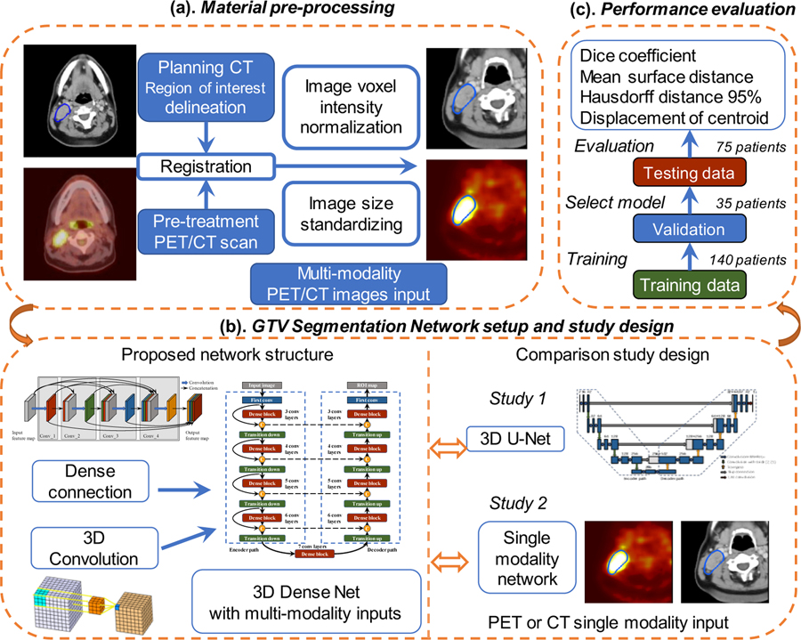
In this work, we proposed a segmentation framework using 3D convolution and dense connections with multi-modality PET/CT images from HNC patients. The overall flowchart of this work is illustrated in Figure 1. Firstly, during the pre-processing step, the planning CT is registered with pre-treatment PET/CT images and the manually delineated GTV contour on planning CT is registered for both image modalities. Normalized and cropped PET and CT images are later on fed into the network. Secondly, we take advantage of 3D convolution and implement dense connections to improve the information flow, reduce network parameters and better utilize extracted features. To demonstrate the effectiveness, the proposed multi-modality Dense-Net is compared with single modality Dense-Net and the 3D U-Net. Finally, the performance of different networks is evaluated by Dice coefficient, mean surface distance, Hausdorff distance 95% and displacement of mass centroid. The details of each module and step outlined in Figure 1 are illustrated in the following sub-sections.

Figure 1.

Flowchart of this study: (a) Material pre-processing; (b) Proposed network with Dense Connections and comparison studies with single modality input and 3D U-Net (c) performance evaluation.

2.1. Materials and pre-processing

The dataset (Martin et al., 2017) of HNC from the Cancer Imaging Archive (TCIA) (Clark et al., 2013) is used in the experiment. It contains ¹⁸F-FDG-PET/CT and radiotherapy planning CT from four different institutions in Québec with histologically proven head and neck squamous cell carcinoma (HNSCC). Patient characteristics are shown in supplemental Table A 1. All patients received radiotherapy with curative intent after the image acquisition. Each patient underwent the ¹⁸F-FDG-PET/CT scan within a median of 15 days (range: 6~80) before the radiation therapy planning. The median total inject dose for PET is 5.0 MBq. CT images are acquired with X-ray tube voltage at 120 kVp. Median follow-up for clinical characteristics is 1309 days (range 245~3402).

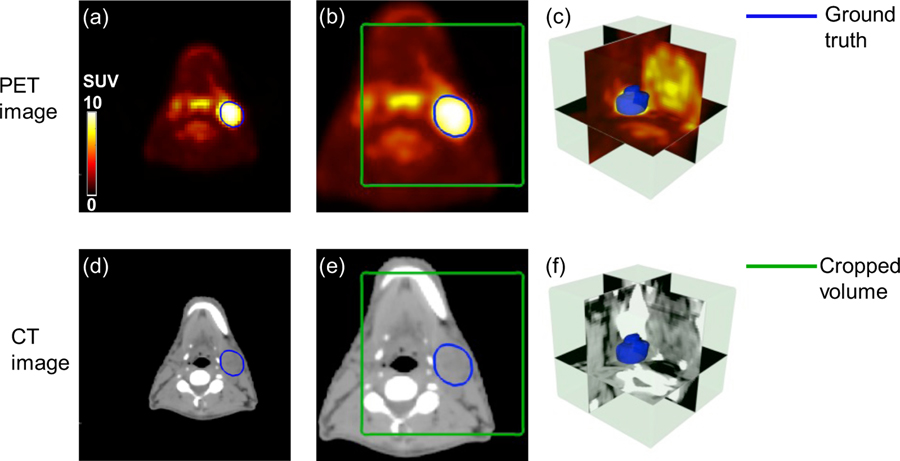
To utilize both anatomic details of CT and metabolic information of PET, images are processed in the following steps. As shown in Figure 2, GTV contours are manually drawn on radiotherapy-planning CT images by radiation oncologists. Pre-treatment ¹⁸F-FDG-PET/CT is registered with planning CT by the automatic deformable registration using the software MIM® (MIM software Inc., Cleveland, OH) (Piper, 2007). The contours originally delineated on planning CT is then propagated to the ¹⁸F-FDG-PET/CT images. The GTV contours, including GTV primary and GTV lymph node, are used as ground truth for the segmentation task. Due to the missing information of some subjects, a portion of the original dataset which consists of 250 patients with both pre-treatment PET/CT and radiotherapy planning CT is qualified in this study.

Figure 2.

Illusive examples of input PET and CT images (blue contour: manually delineated GTV; green box: cropped volume for segmentation). (a) registered original PET image (b) resampled PET image (c) 3D visualization of cropped PET image (d) planning CT image (e) resampled CT image (f) 3D visualization of cropped CT image.

To maintain the consistency across subjects, all PET and CT images are linearly interpolated to the same resolution with a pixel size of 1×1× 2.5 mm³. Due to the large intensity variation among different modalities, the pixel intensity of CT images is normalized to 0~1 according to Hounsfield (HU) window [−200,200] and PET intensity is normalized to the same range using standardized uptake values (SUV) window [0 10]. Considering GPU memory limitation and remove the border black regions, the input 3D-PET/CT image is cropped to a 128×128×48 pixels volume encompassing the GTV annotation by manually select the center pixels as shown in Figure 2 (c, f). All these steps are conducted in MATLAB (2013 Mathworks, Inc).

2.2. Proposed network

CNN is an efficient tool for image analysis and has been widely used for semantic segmentation with remarkable success. Previous studies (Szegedy et al., 2015) have shown that the network depth is a key principle for deep learning architectures. However, the heavy computation burden and memory demand for 3D convolution networks limit the network depth. Residual Networks (He et al., 2016) introduce skip connections within the network, which enables a deeper network. In this work, we implement dense connections and propose a 3D Dense-Net for semantic segmentation, inspired by the original dense network (Huang et al., 2017). This network is composed of dense blocks and transition up/down modules. The details of dense connection are illustrated as following:

X_ℓ is denoted as the output of the ℓ^th layer. In conventional CNN architectures, this vector is typically obtained by applying a non-linear transformation H_ℓ(X) from the output of the previous layer X_ℓ–1,

$$X_{\ell }=H_{\ell }\left(X_{\ell -1}\right),$$ (1)

where H_ℓ(X) is a composite of operations, including convolution, pooling, batch normalization (BN) and rectified linear unit (ReLU). The residual networks integrate H_ℓ(X) with the feature map of previous layer to improve the information flow within the network as

$$X_{\ell }=H_{\ell }\left(X_{\ell -1}\right)+X_{\ell -1},$$ (2)

However, H_ℓ and the feature map are combined by summation, which can impede the information propagation. Pushing the idea of residual connection further, dense connection introduces a more extreme connecting pattern that links a layer to all its subsequent layers by skip connections. In this scheme, the X_ℓ is defined as:

$$X_{\ell }=H_{\ell }\left(\left[X_0,X_1,\dots ,X_{\ell -1}\right]\right),$$

where […] refers to the concatenation operation. This pattern makes each layer in the architecture receives information from other layers, which can alleviate the vanishing-gradient problem, strengthen feature propagation, encourage feature reuse, and substantially reduce the number of trainable parameters. The size of output feature map on each layer is typically set to a small value since it is propagated through dense connections.

This feature-reusing characteristic is quite compelling for medical image analysis tasks, where it is difficult to train a large network with limited training data. In our proposed network, 3D convolution layer is employed to utilize context information from adjacent slices. The convolutional kernel is set to 3×3×3 for computation efficiency. Our final proposed network structure is based on (Jégou et al., 2017) and contains the dense blocks as well as transition-down and transition-up modules. Figure 3 illustrates a dense block with 4 convolution layers. As shown in Figure 3, the left grey cube denotes the original feature map and the output after convolution is represented as the colored cube. The input and output feature maps from the first layer are integrated together and set as the input for the second convolution layer. This process is repeated several times to construct the whole dense block. At last, feature maps from all 4 layers are concatenated together and set as the dense block output.

Figure 3.

Dense block architecture with 4 convolution layers. Blue arrows denote convolutions and black arrows indicate dense connections between feature maps.

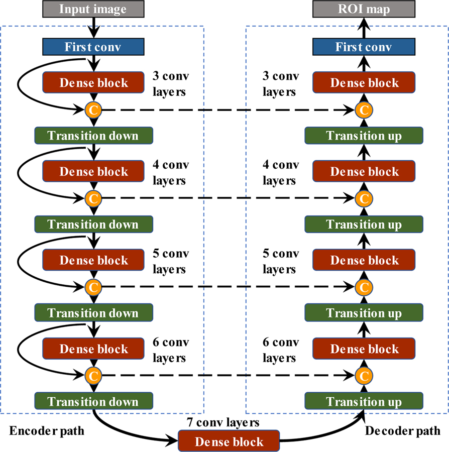
To fully utilize the spatial information of the feature maps, we also introduce transition-down and transition-up modules which are enabled by convolution or deconvolution with stride 2. Figure 4 illustrates the structure of the final constructed network. It is composed of an encoder path to extract contextual features and a decoder path to recover the image details. In the encoder path, we stack four transition-down modules to reduce the spatial resolution and enlarge the receptive fields. While in the decoder path, the image resolution is recovered by transition-up modules to achieve a refined semantic segmentation map. Our network architecture contains 9 dense blocks, 4 transition-down and 4 transition-up modules. For each dense block, it is composed of ℓ convolution layers with feature growth parameter k = 16. The last layer is a 1×1×1 convolution followed by the sigmoid activation function and binarizing threshold value is fixed at 0.5 to generate the pixel-wise possibility map. The details of network parameters employed in each module are summarized in supplemental Table B 1.

Figure 4.

The structure of proposed network including 9 dense blocks, 4 transition-down and 4 transition-up modules.

2.3. Comparison methods

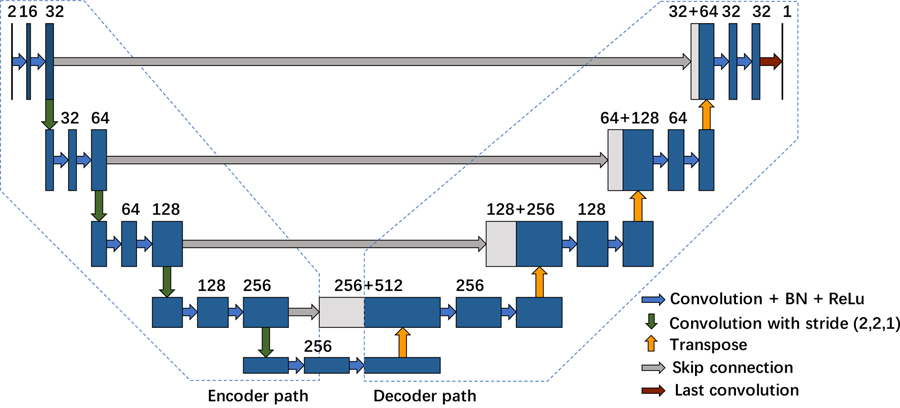
To investigate the effectiveness of the proposed integrated multi-modality segmentation network, we first compared it with single modality Dense-Net using a single modality image as input (PET or CT image alone). Furthermore, the proposed network was also compared with 3D U-Net which is the state-of-the-art for segmentation tasks(Çiçek et al., 2016). 3D U-Net is a classical and widely used architecture for semantic segmentation. It is composed of an encoder path to extract the features and a decoder path to recover the image details. The details of the 3D U-Net employed in our comparison study is illustrated in Appendix C. For each module in the encoder path of 3D U-Net, there are two 3×3×3 3D convolution layers. The feature size is doubled after each module. The exponential growth of feature size in U-Net impeded its extension for deeper networks, as the number trainable parameters become too large when U-Net becomes deeper.

2.4. Evaluation metrics

Multiple metrics are used to quantitatively evaluate the performance of the proposed method. The Sørensen–Dice coefficient (Dice, 1945) is the gold standard for semantic segmentation, which describes the spatial overlap between the ground truth and the network prediction, defined as

$$Dice=\frac{2\left|P\cap G\right|}{\left|P\right|+\left|G\right|},$$ (4)

where P is the set of segmentation results and G denotes the set of ground-truth delineation. |P| or |G| is the number of positive voxels in the binary set and |P ∩ G| is the number of true positive voxels. Although, a higher value of Dice usually denotes a better segmentation result, it depends on the target volume size and the distance between two contours is not considered. Another complementary measurement is the 95th-percentile Hausdorff distance (HD₉₅) (Dubuisson and Jain, 1994), which is employed to measure the distance of the segmentation result.

$$\text{Hausdorff}\hspace{0.17em}\text{distance}=\text{max}\left\{\underset{\text{g}\in \text{G}}{\text{max}}\underset{\text{p}\in \text{P}}{\text{min}}\text{d}\left(\text{g},\text{p}\right),\underset{\text{p}\in \text{P}}{\text{max}}\underset{\text{g}\in \text{G}}{\text{min}}\text{d}\left(\text{p},\text{g}\right)\right\},$$ (5)

where P and G denotes the boundary-surface set of the network prediction and the ground truth, |P| and |G| are the number of voxels in P and G, and d(p, g) indicates the Euclidean distance between voxels p and g. Hausdorff distance refers to the maximum distance of all surface voxels. However, it is sensitive to small outlying object and the 95th-percentile of HD is employed to skip the outliers. A smaller value of HD₉₅ usually denotes a better result. Similarly, mean surface distance (MSD) is defined as follows:

$$\text{MSD}=\frac{1}{2}\left({\text{d}}_{\text{GP}}+{\text{d}}_{\text{PG}}\right)=\frac{1}{2}\left(\frac{1}{\left|\text{G}\right|}{\sum }_{\text{g}\in \text{G}}\underset{\text{p}\in \text{P}}{\text{min}}\text{d}\left(\text{g},\text{p}\right)+\frac{1}{\left|\text{P}\right|}{\sum }_{\text{p}\in \text{P}}\underset{\text{g}\in \text{G}}{\text{min}}\text{d}\left(\text{p},\text{g}\right)\right),$$ (6)

which describes the mean surface distance between the ground truth and the network prediction.

Due to the complex micro-structure around head and neck, we also adopt the displacement of mass centroid (DMC) between ground truth and segmentation result for evaluation. Centroid is the arithmetic mean position of all the points in all of the coordinate directions. A straight-forward estimate of centroid is

$${\widehat{x}}_c=\frac{{\sum }_i^N{x}_i{g}_i}{{\sum }_i^N{g}_i},{\widehat{y}}_c=\frac{{\sum }_i^N{y}_i{g}_i}{{\sum }_i^N{g}_i},$$ (7)

Where (x_i, y_i) are the coordinates of the pixel and g_i ∈ G is the binary ground truth. The summation is over all the pixels relevant to the centroid estimation. Similarly, centroid coordinates of network prediction can be got with same setting. The displacement of two centroids is analyzed by the Euclidean distance with respect to the pixel space on each dimension.

2.5. Experiment setup

This dataset is composed with 250 available patients four different institutions. 75 patients from Centre hospitalier universitaire de Sherbooke (Sherbrooke, QC) is held out for test. The remaining 175 patients is randomly split into training group (140 patients) to train the network and validation group (35 patients) to select the best performance model. Once the model is completely trained, optimised network is then test on independent test dataset with network unseen distribution on 75 patients. Reference methods, including the single modality Dense-Net and the 3D U-Net, are conducted with the same setting. PET and CT images are fed into the proposed network as two input channels and the annotated GTV contours are adopted as the training labels. Each training batch contains one patient’s PET/CT or single modality image. The training data are shuffled at each epoch to increase the robustness. To enlarge the training sample and alleviate the overfitting problem, training images are augmented by applying random translation, rotation (90°, 180° and 270° around y-axis) and mirroring. All the networks are trained from scratch with random weight initialization. The soft Dice (Milletari et al., 2016) which utilize the probability map is defined as follows:

$$Dice=\frac{2{\sum }_i^N{p}_i{g}_i}{{\sum }_i^N{p}_i^2+{\sum }_i^N{g}_i^2},$$ (8)

where p_i ∈ P is the prediction probability for each voxel and g_i ∈ G is the binary ground truth. Soft dice is employed as the training objective function and the Adam algorithm (Kingma and Ba, 2014) with default settings is used as the optimizer. All networks are implemented using TensorFlow 1.4 on a NVIDIA GTX 1080 Ti graphic card.

3. Results

The network is optimized for 100 epochs. It takes around 360 minutes for Multi-modality Dense-Net training. While 3D U-Net with multi-modality image, dense-net with PET and dense-net with CT takes 232, 355 and 355 minutes, respectively. Testing time (i.e. segmentation on new images) of any single or multi-modal network is negligible (<1 minutes).

3.1. Feature map analysis

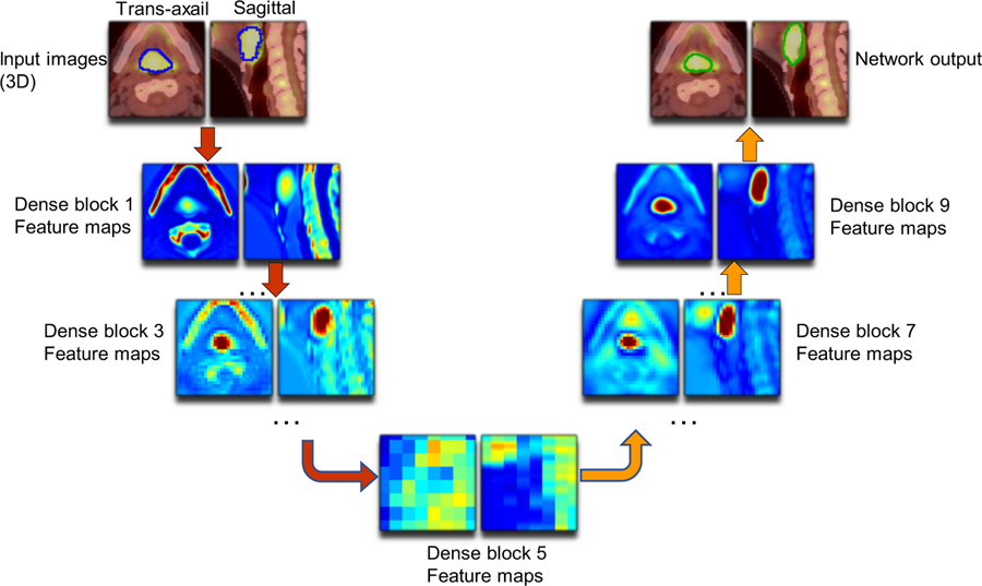
To validate the effectiveness of extracted features, we first visualize the feature map from the output of each dense bock. For each feature map, we use the absolute mean value across different feature channels to illustrate the output. Figure 5 shows an example of the input images and outputs from the dense blocks and explains a clear path of feature propagation and information flow of our multi-modality Dense-Net. As shown, the output at the early block presents high intensity in jaw regions since the voxel intensity of bone is high on CT images. After processed by several dense blocks, the voxel intensity of bone region drops while the tumor intensity is enhanced, which indicates network has learned to automatically select discriminant features from the integrated PET and CT voxels. Meanwhile, the spatial resolution keeps decreasing through the transition-down modules until the bottleneck (dense block 5). Thus, the feature maps extracted from dense block 5 is difficult to interpret. Since high-level features depend on less pixel level information of original image, the features become more abstract as the network goes deeper(Johnson et al., 2016). For the decoder path, the spatial resolution gets recovered by transition-up modules, and the final GTV contour shows up gradually through the following convolution layers. Thus, the final generated segmentation contour (green) recovers the manually delineated GTV contour (blue).

Figure 5.

Representative feature maps from Dense Net (Left: axial plane; right: sagittal plane). Outputs from dense blocks 1,3,5,7,9 are shown for illustration. Blue contours shown on input images refers to the manually drawn GTV (training label) and the green contours shown at the end refers to the network predicted GTV contours (results).

3.2. Qualitative results

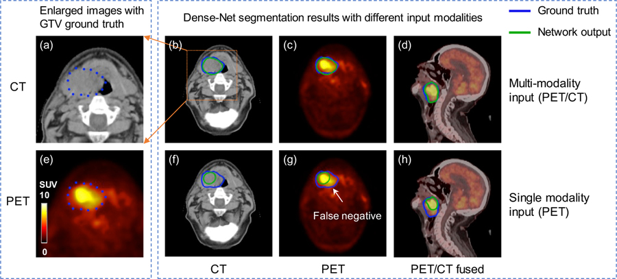
Representative comparison results of Dense Net between single and multi-modality inputs are shown in figure 6. As shown, multi-modality Dense-Net achieves good performance with Dice 0.82 while that of PET single modality input is only 0.60. Tumor voxel intensity is quite high on PET images which can help localize the tumor position, however, the tumor metabolism is heterogeneous and results in the dark region within the GTV.

Figure 6.

Representative results of Dense Net with different input modalities. (a, e) zoomed-in CT and PET images with GTV contours of primary tumor and lymph node. (b, c, d) Dense-Net segmentation results with PET/CT multi-modality input. (f, g, h) Dense-Net segmentation results with PET single modality input. Blue contour represents GTV ground truth and green contour refers to network output.

Fortunately, with the benefit of multi-modality input, our proposed network can delineate this false negative region with the texture information provided by CT images. In comparison, using single modality as input, the network output contour can only follow the PET uptake contour which results in false negative results. This comparison example demonstrates that the output contour from the multi-modality Dense-Net can consider both anatomical and functional information from CT and PET, respectively, leading to superior performance than single modality network.

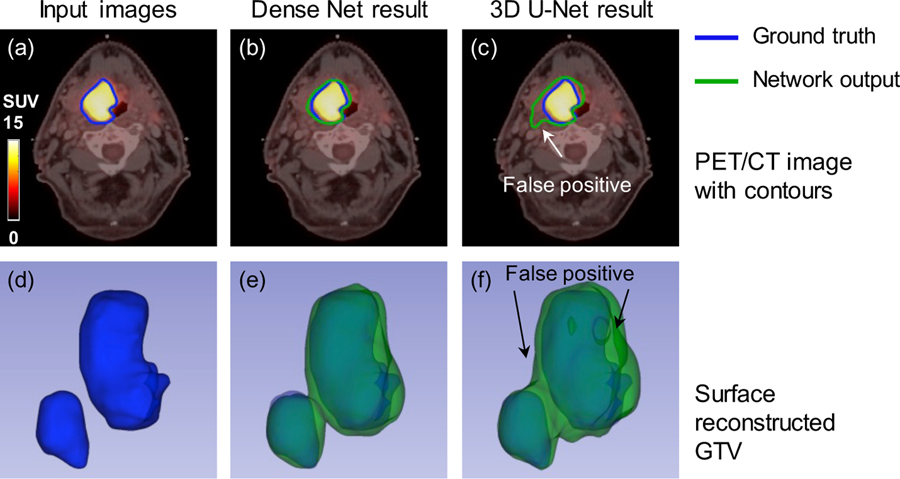
Figure 7 shows another comparison between the proposed Dense-Net and 3D U-Net and mutli-modality PET/CT images are fed into both networks. It is obvious that PET images dominate the segmentation network since PET provide more specific information of tumor region. The result from the 3D U-Net follow this observation and the output contour relies more on PET highlighted regions. Similarly, the anatomical information from CT image can compensate the heterogeneous uptake on PET images. But suitable network is required to extract and take advantage the anatomical information from one channel of input images. The proposed multi-modality Dense-Net (Dice = 0.80) can better delineate the GTV contour compared with the 3D U-Net (Dice = 0.72). The 3D visualization also confirmed that our proposed method can better recover the original GTV, especially in the region pointed out by the white arrow. This might because the convolution layers in Dense-Net can always obtain more information indirectly from the input images by dense connections, due to better information flow.

Figure 7.

Comparison of the segmentation results from the multi-modality Dense-Net and 3D U-Net. (a) Input image; (b) Multi-modality Dense-Net results; (c) the 3D U-Net result; (d, e, f) corresponding 3D visualizations of (a, b, c), respectively.

The network performance on both validation dataset and test dataset measured by Dice, MSD, HD₉₅ and DMC are summarized in Figure 8 and Table 1. Based on result on test dataset, the proposed multi-modality Dense-Net can achieve the Dice median 0.73 with mean and stand deviation (STD) 0.71±0.10, MSD 3.10±1.14 mm, HD₉₅ 8.98±6.34 mm and displacement of centroid 4.82±3.30mm using both PET and CT input images. In the meantime, 3D U-Net yields 0.69±0.11 Dice, 3.57±2.08 mm MSD, 11.16±9.69 mm HD₉₅ and 5.16±3.77 mm displacement of centroid which is relatively lower than Dense Net. When using single modality input, Dense-Net with PET shows dice median 0.64±0.16 (MSD 4.53±3.31 mm, HD₉₅ 14.75±12.17 mm and displacement of centroid 7.82±6.56) which is the lowest among compared methods. Dense-Net using CT as single modality input is also studied, however, the results is extremely low as Dice median 0.32. And the MSD is not applicable to measure the network output using CT single input. Due to the low contrast of soft tissues in CT image, it is almost impossible to apply GTV delineation without complimentary information. Thus, we ignore Dense-Net results using CT single modality in this study. We used right tail paired student’s t-test to assess the significance of difference in the metrics, which means the alternative hypothesis is set as: Dice _{multi-modality Dense Net} > Dice _{comparison method}. It is found that our proposed multi-modality Dense-Net yields statistically better segmentation accuracy over 3D U-Net (p-value = 0.015) and Dense-Net with PET (p-value < 0.001). Besides, the trainable parameters is significantly reduced to 5.58M comparing with 35.3M parameters of 3D U-Net.

Figure 8.

Statistic results of network performance (a) Dice box plot (Box for median and 25~75 percentiles and whisker for 2.5~97.5 percentile), (b) Mean surface distance (MSD), and (c) Hausdorff distance (95%) (HD₉₅), (d) Displacement of center of mass. (b), (c) and (d) shares the same box plot strategy. * stands for p-value < 0.05 and *** for p-value < 0.001.

Table 1.

Segmentation performance metrics comparison for validation and test dataset

Metrics	Method	Dense Net with PET/CT	3D U-Net with PET/CT	Dense Net with PET	Dense Net with CT
Dice	Median	0.73	0.71	0.67	0.32
	Mean ± STD	0.71 ± 0.10	0.69 ± 0.11	0.64 ± 0.16	0.31 ± 0.26
MSD (mm)	Median	2.88	2.98	3.38	-
	Mean ± STD	3.10 ± 1.14	3.57 ± 2.08	4.53 ± 3.31
HD95 (mm)	Median	6.48	7.57	8.29	-
	Mean ± STD	8.98 ± 6.34	11.16 ± 9.69	14.75 ± 12.17
DC (mm)	Median	3.96	4.40	5.56	-
	Mean ± STD	4.82 ± 3.30	5.16 ± 3.77	7.82 ± 6.56

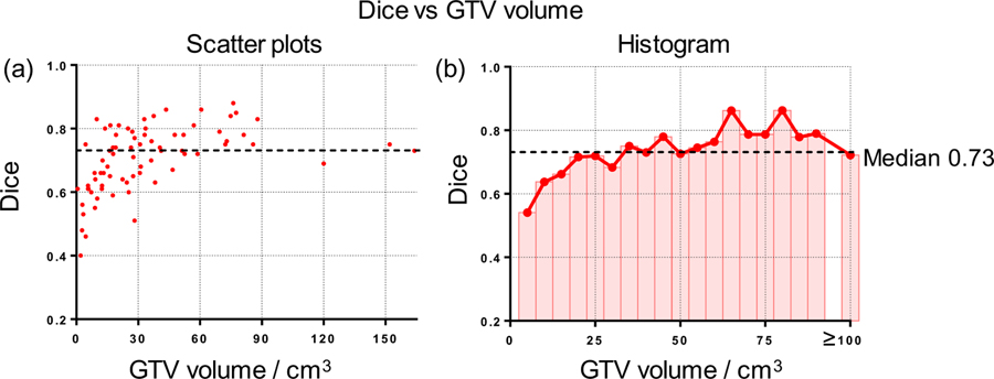
The relationship between GTV volume size and the segmentation performance is also investigated. As shown in figure 9 (a), the larger tumors tend to achieve a better segmentation result with small variance while the segmentation performance is not stable for small lesions. Figure 9 (b) summarized the mean Dice of each size bin (5cm³). For quantitative analysis, we divide patients into two groups accord to its volume size. The Dice result shows significant difference (p-value < 0.001) between large group (volume size > 30 cm³, Dice mean ± STD: 0.75 ± 0.07) and small group (volume size < 30 cm³, Dice: 0.65 ± 0.10). It is obvious that the Dice is affected by GTV volume and small volume results in large variance of Dice value and drives down the overall performance.

Figure 9.

Relationship between Dice and GTV volume size. (a) Scatter plots illustrating Dice and GTV volume size; (b) Histogram and average curve of Dice on GTV volume size.

4. Discussion

In this work, we have proposed a multi-modality segmentation architecture for HNC GTV segmentation. Our results show that the proposed network can learn anatomical and metabolic information from both CT and PET images efficiently and produce better segmentation results compared to state-of-the-art reference methods. Besides, the GTV results based on our proposed network has less variability compared to reference methods, which is crucial for RT applications, where collecting a large number of manually labeled images takes a lot of efforts.

Our proposed architecture employs the 3D convolution and dense connections, which brings several benefits for HNC segmentation task. Firstly, 3D convolution can extract more information across all three dimensions from the volumetric data, which is consistent with the clinical practice where radiologists usually delineate GTV with reference to adjacent slices along the Z-axis. However, the memory consumption and heavy computation burden of 3D convolution limit its application. Then, our proposed network introduces dense connections within the network to conquer this issue and enables each convolution layer access feature maps from all its previous layers. This connection pattern can encourage information and gradient propagation, alleviate the vanishing-gradient problem and reduce the risk of over-fitting. Besides, feature reuse can also reduce the trainable parameters when the network goes deeper, which reduces the risk of over-fitting and is crucial for clinical applications.

Though the performance of our proposed network is better than reference methods, we still observe failure cases during the testing phase which makes the median Dice 0.73, not outstanding other segmentation tasks. One reason is the complexity of HNC GTV segmentation task due to the morphology complexity, and another reason is the still-to-be-improved network structure. Figure 10 shows a set of failure cases with bad segmentation performance. Figure 10 (a) (b) show examples where our proposed network can delineate GTV with highlighted region in larynx following the uptake on PET images. However, since the CT contrast of tumor is not sufficient, the false positive around boundaries increases the denominator and thus achieve a relatively low Dice coefficient (Figure 10 (a): 0.55, (b): 0.62). There are several patients among these cases which can significantly decrease the overall statistics. Besides, we observe that small tumors tend to make low Dice with the small true positive region, and also the Dice coefficient neglects the anatomical significance or relevance of different regions. For instance, a larger tumor has a larger true positive region and a better Dice, without taken the small object into consideration. The Dice of Figure 10 (c)(d) is 0.74 and it suggests a very good delineation result although the lymph node is not recognized.

Figure 10.

Representative cases with false positive and false negative regions. (a) PET/CT image of a patient with tumor in larynx, (b) PET/CT image of a patient with tumor around esophagus, (c) PET/CT image of a patient with large tumor and a lymph node metastasis, and (d) 3D visualization of GTVs in (c).

Due to the limitation of data preparation and implementation, there are still some attempts we can try to achieve better segmentation performance. Firstly, we can further improve the image quality during the pre-processing by refining GTV contours, correcting image artifacts and perfecting the image registration. Secondly, the original image is cropped to 128×128×48 cube due to memory limit. A larger input volume, such as the whole PET/CT image without cropping, might generate better segmentation performance and can be more easily translated to clinics. Besides, additional image modalities can be included in the proposed multi-modality Dense-Net to further improve the segmentation accuracy. For example, magnetic resonance imaging (MRI) are becoming standard practice for HNC with excellent soft tissue contrast, multiplanar imaging capabilities and benefit for dose control. Dual energy computed tomography (DECT) refers to the new simultaneous acquisition of CT performed at two different peak energy levels. Particularly, iodine could be subtracted from contrast enhanced images to improve head and neck cancer image quality, tumor-soft-tissue boundary determination and invasion of critical structures. Pseudo-monochromatic images by linearly combining dual CT can be used to reduce metal artifacts which is especially benefit for head neck cancer. Theoretically, combining these image modalities in our network could better characterize tumor boundaries and provide a robust estimation of target volume estimation.

5. Conclusion

In this study, we have proposed a GTV segmentation framework for HNC radiotherapy. This method employs 3D convolutions to take full advantage of 3D spatial information of images as well as dense connections to improve information propagation from multi-modality images. The proposed multi-modality Dense-Net is successfully applied to HNC patients and achieve satisfying GTV segmentations. The comparison studies demonstrate that our proposed network can achieve better segmentation accuracy than other state of the art methods with less trainable parameters, which show great potentials to assist physicians in radiotherapy planning for a variety of cancer patients not limited to HNC.

Appendix A. Patients characteristics

Table A 1.

Patients characteristics

Characteristics	Total (%)
All patient	250
age (year)
Median (Range)	63 (18~90)
Diagnosis to last follow-up (days)
Median (Range)	1309 (245~3402)
Gender
Male/female	192 (76.8%) /58 (23.2%)
Primary Site
Oropharynx	179 (71.6%)
Larynx	36 (14.4%)
Nasopharynx	18 (7.2%)
Hypopharynx	11 (4.4%)
Unknown	6 (2.4%)
Clinical Stage
I	5 (2.0%)
II	42 (16.8%)
III	62 (24.8%)
IV	140 (56.0%)
Unknown	1 (0.4%)
T stage
T1	31 (12.4%)
T2	93 (37.2%)
T3	83 (33.2%)
T4	37 (14.8%)
Txa	6 (2.4%)
N stage
N0	41 (16.4%)
N1	33 (13.2%)
N2	162 (64.8%)
N3	14 (5.6%)

^aTX: Primary tumor cannot be assessed

Appendix B. Network architecture

Table B 1.

Network parameter

Layer	Output volume	Output feature size	Kernel Size	Stride
First convolution	128×128×48	48	3×3×3	(1,1,1)
Dense block (3 layers)	128×128×48	48+48a	3×3×3	(1,1,1)
Transition down	64×64×48	96	1×1×1	(2,2,1)
Dense block (4 layers)	64×64×48	64+96	3×3×3	(1,1,1)
Transition down	32×32×48	160	1×1×1	(2,2,1)
Dense block (5 layers)	32×32×48	80+160	3×3×3	(1,1,1)
Transition down	16×16×48	240	1×1×1	(2,2,1)
Dense block (6 layers)	16×16×48	96+240	3×3×3	(1,1,1)
Transition down	8×8×48	336	1×1×1	(2,2,1)
bottle neck (7 layers)	8×8×48	112	3×3×3	(1,1,1)
Transition up	16×16×48	112+336	1×1×1	(2,2,1)
Dense block (6 layers)	16×16×48	96	3×3×3	(1,1,1)
Transition up	32×32×48	96+240	1×1×1	(2,2,1)
Dense block (5 layers)	32×32×48	80	3×3×3	(1,1,1)
Transition up	64×64×48	80+160	1×1×1	(2,2,1)
Dense block (4 layers)	64×64×48	64	3×3×3	(1,1,1)
Transition up	128×128×48	64+96	1×1×1	(2,2,1)
Dense block (3 layers)	128×128×48	48	3×3×3	(1,1,1)
Last convolution	128×128×48	2	3×3×3	(1,1,1)

^a+ devotes for skip connection from previous layer output or corresponding dense block

Appendix C. Method for comparison

3D U-Net architecture

BN is abbreviation for batch normalization and ReLU for rectified linear unit.

REFERENCES

- Bagci U, Udupa JK, Mendhiratta N, Foster B, Xu Z, Yao J, Chen X and Mollura DJ 2013. Joint segmentation of anatomical and functional images: Applications in quantification of lesions from PET, PET-CT, MRI-PET, and MRI-PET-CT images Medical image analysis 17 929–45 [DOI] [PMC free article] [PubMed] [Google Scholar]
- Beichel RR, Van Tol M, Ulrich EJ, Bauer C, Chang T, Plichta KA, Smith BJ, Sunderland JJ, Graham MM and Sonka M 2016. Semiautomated segmentation of head and neck cancers in 18F-FDG PET scans: A just-enough-interaction approach Medical physics 43 2948–64 [DOI] [PMC free article] [PubMed] [Google Scholar]
- Berthon B, Evans M, Marshall C, Palaniappan N, Cole N, Jayaprakasam V, Rackley T and Spezi E 2017. Head and neck target delineation using a novel PET automatic segmentation algorithm Radiotherapy and Oncology 122 242–7 [DOI] [PubMed] [Google Scholar]
- Çiçek Ö, Abdulkadir A, Lienkamp SS, Brox T and Ronneberger O International Conference on Medical Image Computing and Computer-Assisted Intervention,2016), vol. Series): Springer; ) pp 424–32 [Google Scholar]
- Clark K, Vendt B, Smith K, Freymann J, Kirby J, Koppel P, Moore S, Phillips S, Maffitt D and Pringle M 2013. The Cancer Imaging Archive (TCIA): maintaining and operating a public information repository Journal of digital imaging 26 1045–57 [DOI] [PMC free article] [PubMed] [Google Scholar]
- Comelli A, Stefano A, Benfante V and Russo G 2018. Normal and Abnormal Tissue Classification in Positron Emission Tomography Oncological Studies Pattern Recognition and Image Analysis 28 106–13 [Google Scholar]
- Deng W, Luo L, Lin X, Fang T, Liu D, Dan G and Chen H 2017. Head and Neck Cancer Tumor Segmentation Using Support Vector Machine in Dynamic Contrast-Enhanced MRI Contrast media & molecular imaging 2017 [DOI] [PMC free article] [PubMed] [Google Scholar]
- Dice LR 1945. Measures of the amount of ecologic association between species Ecology 26 297–302 [Google Scholar]
- Dubuisson M-P and Jain AK Proceedings of 12th international conference on pattern recognition,1994), vol. Series 1): IEEE; ) pp 566–8 [Google Scholar]
- Guo Z, Guo N, Gong K and Li Q Medical Imaging 2019: Computer-Aided Diagnosis,2019a), Series 10950): International Society for Optics and Photonics) p 1095009 [Google Scholar]
- Guo Z, Li X, Huang H, Guo N and Li Q Biomedical Imaging (ISBI 2018), 2018 IEEE 15th International Symposium on,2018), vol. Series): IEEE; ) pp 903–7 [Google Scholar]
- Guo Z, Li X, Huang H, Guo N and Li Q 2019b. Deep Learning-based Image Segmentation on Multi-modal Medical Imaging IEEE Transactions on Radiation and Plasma Medical Sciences [DOI] [PMC free article] [PubMed]
- Harari PM, Song S and Tomé WA 2010. Emphasizing conformal avoidance versus target definition for IMRT planning in head-and-neck cancer International Journal of Radiation Oncology* Biology* Physics 77 950–8 [DOI] [PMC free article] [PubMed] [Google Scholar]
- Havaei M, Davy A, Warde-Farley D, Biard A, Courville A, Bengio Y, Pal C, Jodoin P-M and Larochelle H 2017. Brain tumor segmentation with deep neural networks Medical image analysis 35 18–31 [DOI] [PubMed] [Google Scholar]
- He K, Zhang X, Ren S and Sun J Proceedings of the IEEE conference on computer vision and pattern recognition,2016), vol. Series) pp 770–8 [Google Scholar]
- Huang B, Chen Z, Wu P-M, Ye Y, Feng S-T, Wong C-YO, Zheng L, Liu Y, Wang T and Li Q 2018. Fully Automated Delineation of Gross Tumor Volume for Head and Neck Cancer on PET-CT Using Deep Learning: A Dual-Center Study Contrast media & molecular imaging 2018 [DOI] [PMC free article] [PubMed] [Google Scholar]
- Huang G, Liu Z, Van Der Maaten L and Weinberger KQ Proceedings of the IEEE conference on computer vision and pattern recognition,2017), vol. Series) pp 4700–8 [Google Scholar]
- Jeanneret-Sozzi W, Moeckli R, Valley J-F, Zouhair A, Ozsahin EM and Mirimanoff R-O 2006. The reasons for discrepancies in target volume delineation Strahlentherapie und Onkologie 182 450–7 [DOI] [PubMed] [Google Scholar]
- Jégou S, Drozdzal M, Vazquez D, Romero A and Bengio Y Proceedings of the IEEE Conference on Computer Vision and Pattern Recognition Workshops,2017), vol. Series) pp 11–9 [Google Scholar]
- Johnson J, Alahi A and Fei-Fei L European conference on computer vision,2016), vol. Series): Springer; ) pp 694–711 [Google Scholar]
- Kingma DP and Ba J 2014. Adam: A method for stochastic optimization arXiv preprint arXiv:1412.6980
- Marta GN, Silva V, de Andrade Carvalho H, de Arruda F F, Hanna SA, Gadia R, da Silva JLF, Correa SFM, Abreu CECV and Riera R 2014. Intensity-modulated radiation therapy for head and neck cancer: systematic review and meta-analysis Radiotherapy and oncology 110 9–15 [DOI] [PubMed] [Google Scholar]
- Martin V, Emily K-R, Léo Jean P, Xavier L, Christophe F, Nader K, Phuc Félix N-T, Chang-Shu W and Khalil S 2017. Data from Head-Neck-PET-CT The Cancer Imaging Archive
- Milletari F, Navab N and Ahmadi S-A 3D Vision (3DV), 2016 Fourth International Conference on,2016), vol. Series): IEEE; ) pp 565–71 [Google Scholar]
- Piper J 2007. SU-FF-I-68: Evaluation of an intensity-based free-form deformable registration algorithm Medical Physics 34 2353–4 [Google Scholar]
- Riegel AC, Berson AM, Destian S, Ng T, Tena LB, Mitnick RJ and Wong PS 2006. Variability of gross tumor volume delineation in head-and-neck cancer using CT and PET/CT fusion International Journal of Radiation Oncology* Biology* Physics 65 726–32 [DOI] [PubMed] [Google Scholar]
- Siegel RL, Miller KD and Jemal A 2016. Cancer statistics, 2016 CA: a cancer journal for clinicians 66 7–30 [DOI] [PubMed] [Google Scholar]
- Song Q, Bai J, Han D, Bhatia S, Sun W, Rockey W, Bayouth JE, Buatti JM and Wu X 2013. Optimal co-segmentation of tumor in PET-CT images with context information IEEE transactions on medical imaging 32 1685–97 [DOI] [PMC free article] [PubMed] [Google Scholar]
- Stefano A, Vitabile S, Russo G, Ippolito M, Sabini MG, Sardina D, Gambino O, Pirrone R, Ardizzone E and Gilardi MC 2017. An enhanced random walk algorithm for delineation of head and neck cancers in PET studies Medical & biological engineering & computing 55 897–908 [DOI] [PubMed] [Google Scholar]
- Szegedy C, Liu W, Jia Y, Sermanet P, Reed S, Anguelov D, Erhan D, Vanhoucke V and Rabinovich A Proceedings of the IEEE conference on computer vision and pattern recognition,2015), vol. Series) pp 1–9 [Google Scholar]
- Yang J, Beadle BM, Garden AS, Schwartz DL and Aristophanous M 2015. A multimodality segmentation framework for automatic target delineation in head and neck radiotherapy Medical physics 42 5310–20 [DOI] [PMC free article] [PubMed] [Google Scholar]
- Yu H, Caldwell C, Mah K, Poon I, Balogh J, MacKenzie R, Khaouam N and Tirona R 2009. Automated radiation targeting in head-and-neck cancer using region-based texture analysis of PET and CT images International Journal of Radiation Oncology* Biology* Physics 75 618–25 [DOI] [PubMed] [Google Scholar]
- Zeng Z, Wang J, Tiddeman B and Zwiggelaar R 2013. Unsupervised tumour segmentation in PET using local and global intensity-fitting active surface and alpha matting Computers in biology and medicine 43 1530–44 [DOI] [PubMed] [Google Scholar]