A brain–computer interface for the continuous, real-time monitoring of working memory load in real-world environments

Abstract

We developed a brain–computer interface (BCI) able to continuously monitor working memory (WM) load in real-time (considering the last 2.5 s of brain activity). The BCI is based on biomarkers derived from spectral properties of non-invasive electroencephalography (EEG), subsequently classified by a linear discriminant analysis classifier. The BCI was trained on a visual WM task, tested in a real-time visual WM task, and further validated in a real-time cross task (mental arithmetic). Throughout each trial of the cross task, subjects were given real or sham feedback about their WM load. At the end of the trial, subjects were asked whether the feedback provided was real or sham. The high rate of correct answers provided by the subjects validated not only the global behaviour of the WM-load feedback, but also its real-time dynamics. On average, subjects were able to provide a correct answer 82% of the time, with one subject having 100% accuracy. Possible cognitive and motor confounding factors were disentangled to support the claim that our EEG-based markers correspond indeed to WM.

Introduction

Working memory (WM) is a system that stores, maintains and process information while a person performs any cognitive task, from keeping a phone number in mind to engaging in speech comprehension. It works as an interface between perception, long-term memory and action (Baddeley 1992).

Baddeley proposed a multicomponent model to explain the mechanisms of WM. The individual components of this model are the visuo-spatial sketchpad, the phonological loop, the episodic buffer and the central executive. The visuo-spatial sketchpad and the phonological loop handle visual and auditory information, respectively, whereas the episodic buffer holds pieces of combinations of taste, smell, visual and acoustic data (Baddeley 2017). The central executive has a coordinating role concerning the visuo-spatial sketchpad, the phonological loop and the episodic buffer.

The capacity of WM is limited (Sweller 2011), and WM load (or cognitive load) is regarded as the amount of resources required to perform any given cognitive task. According to Cognitive Load Theory, cognitive load has a pivotal role in successful learning and intellectual performance (Paas et al. 2003). For instance, WM overload might lead to accidents; as an example, it has been studied in air traffic controlling (Shorrock 2005). In addition, prolonged high cognitive load leads to fatigue (Mizuno et al. 2011), which is, in turn, linked to common accidents that could be prevented with the help of real-time monitoring systems (Zeng et al. 2018). Thus, the applications of a continuous, online (real-time) WM estimation could range from learning to security.

To investigate the neural correlates of cognitive functions, it is necessary to image the brain. Several brain imaging techniques, e.g., magnetic resonance or electroencephalography, are used by researchers in order to infer structural and functional properties of the brain.

For real-time applications on healthy users, EEG is an interesting technique due to its high temporal resolution, non-invasive nature and low acquisition and operational costs. In particular, in this study we are interested in cognition, which might induce sustained activity, as opposed, for instance, to motor activity that takes place during a short period of time.

The biomarkers used in our BCI are derived from EEG spectral properties (see “The EEG biomarkers: spectral changes in EEG due to WM load”, “Offline study: designing the BCI” sections). Changes in the spectral properties of EEG in response to a varying WM load were observed previously by other authors. Sauseng et al. (Sauseng et al. 2005a) report alpha synchronization in the prefrontal areas, with alpha desynchronization in the occipital areas. In a different study (Sauseng et al. 2005b) they report increased theta long-range coherence and decreased anterior upper-alpha short-range connectivity for increasing demands on the central executive. Jensen and Tesche (2002) found that theta power at frontal electrodes increases as a function of the number of items stored in WM. More generally, Antonenko et al. review the use of EEG for measuring cognitive load (Antonenko et al. 2010). Cavanagh argues that theta band activity might entail computation required for cognitive control (Cavanagh and Frank 2014).

Beyond spectral properties, we previously reported how cognition changes brain dynamics in a manner that can be observed directly in the EEG statistical properties (Mora-Sánchez et al. 2019). An example of the use of EEG-derived markers to screen non-cognitive conditions is the study of Mumtaz et al. on alcohol use disorder (Mumtaz et al. 2017).

We developed our system in the framework of BCIs. A BCI is in general a device that allows humans to interact with machines by directly using brain activity, bypassing the motor system (Wolpaw et al. 2000). These devices take neuroimaging signals as an input and generate a desired output via a translation algorithm. The output is often a command that helps the user in either conveying a message or controlling an object. For instance, choosing a letter in the first case, or moving a wheelchair in the second case (Farwell and Donchin 1988).

BCIs were initially designed for patients whose conditions have impaired their main communication or command channels, such as speech or the motor system. Locked-in patients (Hinterberger et al. 2003) or paralysed patients (Muller-Putz and Pfurtscheller 2008) are typical examples. In healthy subjects, however, regular speech is an efficient way of communication. Besides, the motor system provides a fine-tuned means of control with a high number of degrees of freedom. Both the motor system and speech demand relatively low cognitive effort compared to BCI. Nevertheless, BCI systems can go beyond communication and control; they can be useful for cognitive monitoring as well, as suggested by Müller et al. (2008).

Zander and Kothe (2011) conceptualised a new way of using BCI. They propose a new classification of BCI by the type of mechanism used to achieve control of the device: conscious voluntary control (active BCI), conscious voluntary control aided by external stimulation (reactive BCI), or non-intentional control (passive BCI). The system developed here is a passive interface.

The goal of a passive BCI is to improve the performance of a system by obtaining contextual information about the cognitive state of the user. Such information is provided in a way that is non-voluntarily driven by the user. Passive BCIs have been used mostly in offlines analyses for various applications, such as flight and driving monitoring (Dehais et al. 2019; Di Flumeri et al. 2018; Borghini et al. 2014) and object recognition (Tafreshi et al. 2019). Having this information, appropriate commands can be triggered, allowing the system to adapt to the user. In the case of healthy users, passive BCI could be of special interest in improving human–machine interactions (HMI). Furthermore, beyond HMI, feedback-based learning in general may greatly benefit from neurofeedback protocols (Gaume et al. 2016).

In operational terms, we expect to design a system able to monitor WM in a continuous manner, on the order of a few seconds.

The present study is based on the work of Gaume et al. (2019) and on a preliminary offline classification results reported for a smaller database (Mora-Sánchez et al. 2015). It is an extension including real-time validation, real-time neurophenomenological validation on a cross task, the disentanglement of potential confounding factors (motor and cognitive) and a larger number of subjects.

Neurophenomenological validation refers to subjects confirming the agreement between their subjective experience and an objective measure proposed as a correlate to that experience. Although the main goal of neurophenomenology (Varela 1996) is beyond the scope of this study, it has interesting proposals regarding the relationship between subjective experiences and their objective, physical substrates. Lutz (2002) provided the first case study in which first-person (subjective experience) and third-person (objective measures) data are related in the context of neurophenomenology.

A cross task is a necessary condition if we intend to generalise our findings to real-world environments. A BCI that truly measures the load of the central executive trained on a given WM task, should be able to transpose the classification of the same load on a different WM task.

Finally, disentangling confounders (see “Online control tests: disentanglement of potential confounding factors” section) through control tests is crucial to support the claim that our EEG biomarkers correspond specifically to WM and not to correlated electrical activity of brain or muscle origin. For a discussion of the importance of cross tasks and of disentangling confounders in a WM BCI, the reader can refer to Gerjets et al. (2014). Our hypothesis in this regard is that WM-load estimations will not be high when subjects are instructed to perform actions that are less demanding of WM, but where the presence of confounders is evident (more details in “Online control tests: disentanglement of potential confounding factors” section).

The confounding factors controlled in this study were attention, attentional filters, internal speech, sub-vocalization, frustration and arousal. Attention and attentional filters are indeed part of WM under some models (Cowan 1999), but do not encompass the whole construct of WM. A relevant approach in this regard is that of Vogel et al. (2005), who show evidence suggesting that individual differences in WM capacity might be at least partially explained by individual differences in filtering efficiency. Individuals with a low WM capacity may have less efficient filtering mechanisms, which can lead to deficient encoding strategies and the consequent storage and maintenance of irrelevant information.

The tasks developed in this study involved the phonological loop (Baddeley 1992); therefore we need to disentangle potential correlates of internal speech and sub-vocalization. In addition, frustration is known to be highly correlated with mental effort (Paas et al. 2003). Eye-blinks and other visible electromyographic artifacts were removed from the learning set in order to prevent biasing of the model (see “Offline study: designing the BCI” section).

Materials and methods

Initial WM task

To feed the subsequent algorithm, we collected an EEG database of subjects performing a WM task with two different conditions (high and low WM load), corresponding to the classes that the algorithm was meant to learn to discriminate. Ideally, both conditions should differ only in the amount of WM load induced (see “Online control tests: disentanglement of potential confounding factors” section for a detailed discussion).

The task, which will be referred to as Task 1, is described below.

• Subjects sit in front of a computer screen and are presented with a collection of figures that will be used during the experiment. They are asked to assign a short name to each figure, to become familiar with the set. There are different sets of figures, and each set corresponds to a different semantic field: animals, vehicles, geometric shapes, etc (see “Appendix 1: Images used for Task 1” section for details).

• The target to be memorised appears on the screen. The target is a specific sequence of the previously displayed figures. There are two conditions, one in which the target contains two figures (low-WM-load condition), and a second condition in which the target length is five or six figures (high-WM-load condition). The number of figures in the high condition was determined for each subject depending on their WM span after performing 21 preliminary trials.

• The target disappears and a sequence of figures, generated from the same semantic field, slides from right to left on the screen. The sliding speed is 222 pixels per second. The subjects have to press a button whenever they find the target within the sequence. This is considered one trial. If the subject presses the button before the target appears or if they miss the target, the trial is over and is not analysed, to prevent including in the analysis trials with an unknown WM load. Trials last on average 25 s. An example of low-load trial is shown in Fig. 1. Subjective feedback about frustration is collected after each successful trial by means of an analogue Likert scale (unsuccessful trials are automatically discarded to guarantee that the subjects actually followed the protocol, as explained above). The question was taken from the NASA Task Load Index questionnaire (Hart and Staveland 1988).

• A new target (belonging to the other WM condition) is shown and the whole process repeated. Both conditions are alternated to prevent the BCI from learning slow EEG drifts that are WM independent.

Fig. 1.

Representation of the low-WM-load task

The fact that subjects were asked to assign a short name to each figure induced in them a simple storage-retrieval technique: to internally repeat [using the phonological loop (Baddeley 1992)] the names of the elements of the target and to compare them with the observed sliding items. Subjects were indeed instructed to do this to ensure a homogeneous encoding strategy. The choice of this particular encoding strategy was the result of a preliminary analysis, in which subjects reported this use of the phonological loop to be the most natural encoding strategy. If subjects are not instructed to maintain a homogeneous strategy, the strategy can evolve to reduce the WM load for a given task.

As an example, according to Ericsson and Delaney (1999), in a digit span task, the typical initial strategy is simply to rehearse groups of numbers. As subjects become familiar with the task and obtain expertise, the encoding strategy moves towards associating numbers with their own pre-existing knowledge. The authors describe how a subject with a normal memory span develops a (task-specific) span far beyond the limits of WM. The encoding strategy exploited information with which the subject was familiar: racing times (the subject was very interested in racing sports, and hence he dealt with racing times often).

It was crucial in our experiment to prevent subjects from developing such strategies for several reasons: first, to have a constant WM load; second, to reduce variability, as the potential encoding strategies are as different as the body of knowledge of every subject; and finally, because we do not want to involve long-term memory. Mnemonic techniques, for instance, use long-term WM structures for the retrieval of information (Kintsch et al. 1999). A particular strategy of this kind, observed in preliminary tests, was to create short stories. Therefore subjects were specifically instructed not to do so. To further discourage this possibility, all the figures belonged to an evident semantic field. To reduce habituation, the semantic field changed.

For estimating the WM span of the subjects and the associated length of the target, subjects performed 7 trials for each of 3 different semantic fields (“Appendix 1: Images used for Task 1” section). For the actual recordings, subjects performed 10 trials for each of 4 different semantic fields.

WM is a construct not only responsible for information storage, but also maintaining and processing (Baddeley 2003). We focused on these three sub-functions of WM. Storage is controlled by the design of the experiment, as both conditions differ in the number of items to be remembered. However, the maintaining and processing loads are harder to impose and monitor without largely complicating the experiment. Therefore, subjects were instructed to internally maximise the difference in both conditions regarding these two remaining aspects.

In the high-WM-load condition, they were asked to internally refresh the items as fast as possible (fast and continuous internal speech), and to perform the processing (figure comparison) as intensively as possible. An intensive comparison being, for example, not only deciding if the items are different, but finding some differences such as the number of lines. For the low-WM-load condition, they were asked to do the opposite, slow refreshing and low processing.

Before the actual recordings, subjects were left to interact with the system to gain familiarity with the instructions and in particular with this maximization strategy. As pointed out by Lotte et al. (2013), the effectiveness of feedback partly relies on the clarity of instructions and goals.

Distracters, or sequences similar to the target, prevent the use of memorization strategies focusing on subsets of the target. Distracters appear naturally for targets with 2 figures, however, it is unlikely that distracters will appear by chance for targets with 5 figures or more. Hence, the randomized sequence was generated so that distracters appeared exactly in 50% of the trials. As distracters appear randomly only half of the trials, subjects do not learn to expect the target after a distracter. A distracter was defined as a pattern similar to the target, differing only in one item that could be located in any position from the third onwards.

The duration of each trial is a random number between 15 and 30 s. A random value prevents subjects from implicitly learning the task length instead of performing the task itself, which would severely bias the results.

The area on the screen where the figures slid was $100\times 300$ pixels; the size of the figures was $100\times 100$ pixels. The small window size reduces eye movements, which are known to produce artifacts. Because of the size of the area, the size of the figures, and the sliding speed, subjects could only see one complete figure at a time. The experiment was written in Matlab 2015a using Psychophysics Toolbox extensions (Kleiner et al. 2007).

The distance between the subjects and the screen was 60 cm and, considering their 100 pixels size, the figures subtended a visual angle of 2.53°. The screen model was ProLite E2208HDD. Lighting and noise conditions were normal office conditions.

A photodiode connected directly to the EEG amplifier auxiliary input allowed synchronization between the EEG recordings and the visual stimulation. The BPW-21R photodiode was chosen for its sensitivity to visible light (420–675 nm) and its theoretical response time of about 3 μs, lower than any other time scale in our setup.

BCI design and implementation

The end goal of this study is to estimate the probability that a subject is experiencing either high-WM load or low-WM load, by using subject’s EEG data acquired on the fly. We chose to perform the estimation of the above probability with a machine learning classifier. A classifier predicts the class membership of an element based on a set of known examples. The training of a classifier requires then a previously recorded (offline) dataset composed of segments of EEG (examples) with known corresponding WM-load values (labels).

The offline dataset was obtained by recording 20 subjects performing Task 1. In total, 1744 examples (59% low-WM load and 41% high WM-load) with known labels were analysed offline to design the classifier. The reader interested in technical details can consult the “Offline study: designing the BCI” section of the Appendix.

The above classifier is part of a pipeline able to take EEG as input and provide as output an estimate of the WM load. The online classification performance however could be lower than that of its offline counterpart due to over-fitting for instance. Online, as all the data are completely independent from the learning data, there is no risk that positive effects may be the result of over-fitting. In addition, only online it is possible to inquire about the subjects’ cognitive state to perform neurophenomenological validation.

The next section describes the online tests performed with the classifier designed offline. Technical details of the online BCI system can be found in the “Online analysis: from EEG recordings to a WMLE” section of the Appendix.

Online tests: the calibration session

After the offline analysis of the first 20 subjects was completed, new subjects were recruited for online tests.

For each of the new subjects, a small session was devoted to customise the classifier prior to the online recordings in a calibration session. In the calibration session, subjects performed Task 1 and their EEG data were processed in the same manner as the data collected offline.

The calibration session led to the collection of 45 low-WM examples and 45 high-WM examples per subject, and these 90 examples were added to the offline data before training the classifier. An instance of the classifier depends on the data that were used to train it, and therefore the classifier used for each user was different. Nevertheless, all the classifiers were built by following the same rules, that correspond to the set of parameters found to be optimal in the offline analysis, as described in the “Offline study: designing the BCI” section of the Appendix.

Any instance corresponding to a classifier trained with the offline data plus the calibration data will be referred to as the classifier C.

Online tests: BCI validation

To validate the classifier with completely independent data, subjects continued performing Task 1 after the short calibration session, but this time the analysis was carried out online. We will refer to this test as the BCI validation.

Once the online session started, the classifier C was used to analyse the stream of incoming EEG data. The output of the classifier C was the estimated probability that the current EEG epoch corresponded to high-WM load (the posterior probability (Nasrabadi 2007) of the classifier), which will be referred to as the WM-load estimate (WMLE). This value, being a probability, is a continuous number between 0 and 1, small for a typical low-WM-load EEG epoch, and large for a typical high-WM-load epoch.

With the WMLE values, a receiver operating characteristic (ROC) curve was computed to assess the performance of the classifier. A ROC curve is a plot of false-positive versus true-positive rate for different threshold values [for details see for instance (Swets 2014)]. The threshold is the value of the WMLE above which we consider an EEG epoch as corresponding to a high-WM-load state. The area under the curve (AUC) of a ROC curve is a useful indicator of the performance of a classifier. AUC values have a value of 0.5 for a random classifier and an upper bound of 1 for a perfect classifier: the larger the value, the better the classifier.

Each subject performed 20 trials, except one who, due to his own time constrains, performed only 6 trials. Trials were divided, as in the offline analysis, in non-overlapping epochs of 2.5 s.

Online tests: neurophenomenological validation on a cross task

A second group of online tests followed the BCI online validation, the aim of these tests was to validate the reliability of the system on an entirely different, yet WM-based task (a cross task). Performing a cross-task is necessary to control task-related confounders (Gerjets et al. 2014), and therefore to support eventual generalizability of the findings.

The classifier C, trained on Task 1, was used to predict the WM load of the subjects in a mental arithmetic task, which imposed a high demand on the processing component of WM (Cragg et al. 2017). During this task, which we will refer to as Task 2, subjects were instructed to perform arithmetic computations (details in “Appendix 3: Arithmetic operations in Task 2” section) while a visual cue was shown on the screen. After 8.5 s, the visual cue disappeared and subjects stopped the mental arithmetic; the trial lasted for 11.5 extra seconds after the visual cue disappeared.

The classifier C analysed the stream of EEG data to provide a WMLE, as in Task 1. Unlike in Task 1 however, the WMLE was used to display real-time (every 150 ms) continuous feedback, in the form of a gauge whose height was proportional to the WMLE. The gauge was shown throughout the whole trial (except for the first 2.5 s, as the buffer of the classifier C requires 2.5 s of data to produce an output).

The ability of the system to provide an meaningful objective measure of the subject’s cognitive state was assessed via neurophenomenological validation. This validation took place after each mental arithmetic trial, where subjects were asked to decide whether the feedback provided by the gauge matched the dynamics of their subjectively perceived WM load. Subjects had to complete the sentence I believe that the feedback gauge was... with one of the following sentences: (a) correlated with my WM load, (b) not correlated with my WM load, or (c) I don’t know.

To prevent an optimistic estimation due to a potential obsequiousness bias, half of the time sham feedback was provided. Subjects were aware that the aim was to validate whether the feedback was indeed reflecting their load, and that half of the time we would provide sham feedback. Sham feedback took the form of a reversed estimate, i.e., a large bar when the WMLE was a low and vice-versa. A reversed gauge has the advantage that its dynamical behaviour cannot be distinguished from the real feedback dynamics.

Neither these questions nor the instructions given to the subject mentioned that the sham feedback was reversed. This information was withheld to prevent subjects from being tempted to devote their cognitive resources to invert their estimations and evaluate whether they matched with the feedback.

Ultimately, what we evaluated was the subjects’ ability to decide whether the feedback was real or sham, which in turn assesses the reliability of the BCI, provided confounders are disentangled.

Each subject performed 20 trials, except for one, who due to own time limitations performed only 10. Before the actual recordings, there was a training session with 3 trials using the real estimation and 3 trials using the reversed estimation. The number of trials per subject in this training session was set relatively low to avoid a potential bias due to cognitive fatigue.

Online control tests: disentanglement of potential confounding factors

The last online tests were control tests aiming at disentangling potential confounding factors. These tasks were designed in such a manner that the confounders are present, but the task itself demands a low WM load. The response of the classifier C (we do not call this response the WMLE because we are performing control tests) was the statistically compared with the WMLE of the low-WM-load trials.

The confounders analysed were attentional filters, attention, internal speech, sub-vocalization, and frustration. Three control tasks, described in the next section, covered these potential confounders. In addition, arousal was analysed offline, and eye-blinks were removed from the learning database; see “Offline study: designing the BCI” section.

We mentioned in “Online tests: BCI validation” section the requirement of a task with two conditions, differing only in the amount of WM load imposed on the subject. In practice, as WM is a multimodal complex construct, there might be confounding factors involved, i.e., factors unspecific to WM, or task-dependent, that change across conditions (Gerjets et al. 2014).

Unspecific factors can be motor or cognitive confounders, such as frustration, attentional filters, eye-blinks, sub-vocalization or muscle contractions. These confounding factors might or might not be part of the WM construct, but they do not encompass the whole construct and basing a classifier only on them would be misleading. On the other hand, cross-task is meant to remove task-dependent factors.

Figure 2 is a graphical representation of the process of confounder disentanglement. The plane containing the ellipses is an abstract plane representing EEG biomarkers, with no particular order within the plane. The leftmost ellipse represents the set of biomarkers that change across conditions in Task 1. The rightmost ellipse correspond to biomarkers that change across conditions in Task 2. The upper vertical ellipse depicts biomarkers that change when a subject experiences high WM load, while the remaining ellipses represent biomarkers that change under the presence of the respective confounders.

Fig. 2.

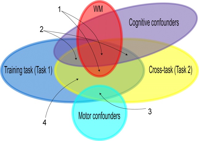
Confounders to be disentangled. The plane represents EEG biomarkers. Each ellipse is the set of biomarkers that change across conditions (for Task 1 and Task 2), or that change whenever the associated notion is present (WM, motor confounders and cognitive confounders). Area 1 represents the ideal WM markers. Area 2 represents (cognitive) activity necessary but not sufficient for WM. Area 3 represents potential motor confounders. Area 4, the remaining part of the crosshatched area, should be empty if all the potential confounders were correctly identified

If a classifier is trained with data from Task 1, and tested with data from Task 2, the EEG biomarkers that trigger a high response of the classifier (with the test data) are represented by the intersection of the leftmost and rightmost ellipses in Fig. 2. These biomarkers are ideally task independent, due to the difference in nature between the tasks. However, this set of biomarkers is not free from biomarkers elicited by confounders and therefore we need to disentangle them.

In Fig. 2, area 1 represents the ideal set of biomarkers. Area 2 contains cognitive activity necessary but not sufficient for WM, such as attention, that could potentially be shared by both tasks and change across conditions. Area 3 contains potential motor confounders that could also be shared by both tasks and change across conditions, like sub-vocalization. After all the confounders have been identified, the remaining part of the ellipse, area 4, should be empty.

The recordings of a subject systematically producing electromyographic artifacts during the high-WM-load condition of both tasks (see “Confounding factors” section) belong to this area, and were therefore discarded from the results. According to the embodiment theory (Varela et al. 2017), the ellipses concerning cognitive activity and motor activity might not be disjoint. However, we are not considering this hypothesis in this work.

Disentangling cognitive confounders that are thought to be a component of WM is extremely important, as relying heavily on single elements of WM would pose difficulties for postulating biomarkers, as well as for generalizability.

Our working hypothesis is that if the design, implementation and analysis of Task 1 was methodologically correct, supervised machine learning algorithms should be specific enough to trigger a high response only when the whole construct of WM is engaged.

In general terms, our experimental design addresses task independence and WM-specificity in the following manner. The performance of the online cross-task is meant to support the claim that the markers are task independent. In addition, if the online control tasks that are designed to trigger confounders do not elicit a response in the classifier (statistically different than the classifier’s response to a low WM-task), then these confounders are not playing a major role in the set of biomarkers.

First online control test: attentional filters

Attentional filters are a sub-component of WM under certain models as explaiend in the introduction, furthermore, some authors have reported experimentally an interaction between WM and selective attention (Downing 2000; de Fockert et al. 2001).

To address this problem, we designed a task identical to the low-WM-load condition of Task 1, with one difference. Above the sliding figures where the target was contained, the picture of a red fly followed a chaotic trajectory for a random duration between 1 and 2 s. Subsequently, it would spin around for another random duration between 1 and 2 s. The fly alternated between these behaviours. This extra item, spanning the visual field with an unpredictable motion, forces the subjects to make greater use of their attentional filters to succeed.

The aim of this task was to test whether the attentional filters elicited part of the EEG biomarkers found. Twelve trials were performed for this test.

Second online control test: attention

Attention has been reported as well to interact with WM (Awh et al. 2006), and therefore it needs to be controlled as a potential confounding factor.

For the second control task, targeting attention, subjects performed a visual reaction time test. The goal of the test was to press a key whenever a visual cue appeared on the screen. As the cue appeared at random times, subjects needed to be attentive to press the key at the correct time. Ten trials of 10 s each were performed.

Third online control test: internal speech and sub-vocalization

Internal speech is a fundamental part of Baddeley’s model through the phonological loop, in addition, one’s inner voice produces muscular activity that can contaminate EEG recordings. In fact, researchers have been able to translate these signals into speech (Mohanchandra and Saha 2016).

A third control task, targeting internal speech and sub-vocalization, involved subjects internally repeating slowly and continuously a lengthy word of their choice, depending on their native language. Ten trials of 10 s each were performed.

Online control tests: hypothesis testing

At this point, we had already saved the WMLE values of subjects performing Task 1 in low-WM-load condition. Our null hypothesis was that if our EEG biomarkers are specific to WM, then potential confounders would not trigger a high response of the classifier C. Therefore, the null hypothesis translates to the following: the response of the classifier C from control tests is not higher than WMLE values from Task 1 in low-WM-load condition.

Failing to reject the null hypothesis after an adequate statistical test would then support the claim that our BCI is WM specific. Such test was a paired Student t-test, given that the same set of subjects performed Task 1 and the control tests.

Subjective information about frustration was collected after Task 1 trials. As mentioned in “Initial WM task” section, this information was collected via an analogue Likert scale. For each trial, the mean value of the WMLE was compared with the subjective frustration level provided by the subject. A possible correlation between these two values was studied using a conjunctive analysis including Bonferroni corrections (Vialatte and Cichocki 2008). This method, previously proven useful for EEG, assesses statistical significance without losing statistical power when performing multiple hypothesis testing, each subject being a test in this case. A lack of correlation would support a lack of effect of frustration on the WMLE.

Potential confounding factor analysed offline: arousal

During previous tests of subjects performing Task 1, some of them reported an arousal effect when distracters or when the target appeared. Data flagged as potentially containing arousal was removed from the learning set, as mentioned in “Offline study: designing the BCI” section. However, despite the fact that the system was not expected to have learned arousal as a marker, we decided to test whether online recordings could be classified, offline, with known arousal markers.

It has been reported in the literature that reliable markers of arousal are an increase in central frontal beta activity (Haenschel et al. 2000), a decrease in central frontal theta activity (Strijkstra et al. 2003), and an increase in global alpha activity (Strijkstra et al. 2003). To test the effect of arousal, we decorrelated from the output of the classifier the information contained in these markers. The latter was done by performing Gram-Schmidt orthogonalisation (Cheney and Kincaid 2009).

We tested this approach by classifying our offline database. If our classifier is based on arousal, after decorrelating these markers of arousal we expect classification performance to drop to chance levels. If it is not based on arousal, we expect only a slight variation in the classification accuracy.

Data acquisition

Brain activity was recorded using a 16-channel EEG device (Brain Products V-Amp) at a sampling rate of 500 Hz. The electrode set-up is shown in Fig. 3. Two groups of subjects participated in the study. The first group of subjects was recruited for the offline analysis (see “BCI design and implementation” section) . The second group of subjects was recruited for the calibration session (“Online tests: the calibration session” section) and the subsequent set of online tests (“Online tests: BCI validation” section).

Fig. 3.

Electrode setup

Concerning the first group, 20 healthy subjects between 21 and 31 years of age were recorded, 10 males and 10 females. Sixteen of these subjects were right-handed, 3 were left-handed, and for one of them the information is missing. The second group consisted of 9 subjects, 5 males and 4 females. Eight subjects were right-handed and one subjects was left-handed. The online BCI validation was performed by all of them. Six of them, 3 males and 3 females did the cross task. Confounder disentanglement tests were performed on 4 subjects, 2 males and 2 females.

After completion of each test, subjects were asked if they had experienced mental fatigue. If they responded affirmatively the experiment was stopped, which was one reason why not all the subjects performed the full test battery. In addition, one subject was lost due to illiteracy after BCI validation (“BCI validation” section). One subject did not perform the neurophenomenological validation (cross task) due to cognitive difficulties manifested by the subject while performing the task (see the discussion section for more details).

All subjects had normal or corrected to normal vision and the absence of any brain disorder or drug consumption. The study followed the principles outlined in the Declaration of Helsinki. All participants were given explanations about the nature of the experiment and signed an informed consent form before the experiment started.

All the EEG epochs analysed were 2.5 s long. For the offline training data, a total of 1744 non overlapping windows were analysed, 59% corresponding to a low-WM load. The reason why there were more low-WM-load epochs available offline is the length of the distracters. Distracters in the high-WM-load condition last longer, and therefore less distracter-free epochs were available in the high-WM condition.

Online tests were performed on the continuous stream of EEG data, therefore online the data corresponding to low and high WM-load was balanced.

All the results presented in this study are online, hence as the classes are balanced the chance level regarding classifier accuracy is 50%.

Results of the online tests

BCI validation

A 2-parameter ROC curve for the 9 subjects was generated using the 126 artifact-free, successful trials of Task 1 online. The usual parameter in a ROC curve is the classification threshold; however, an additional parameter was relevant: the required sustained activity.

In this study there is a continuous estimate, in other words, a set of WMLE values over time for each trial instead of a global estimate of the WM load. We can, for instance, classify a trial as corresponding to high-WM load only if the activity stays above the threshold for a certain duration. Therefore, for every threshold and for every required time (each pair being a possible BCI design) a sensitivity-specificity pair is available. Values are displayed in Fig. 4 for the whole set of subjects. The curve is thick because of the two parameters.

Fig. 4.

2-Parameter ROC curve for the Task 1 performed online. The curve has thickness because there are two parameters: the classification threshold and the required time of sustained activity. Each point represents a possible BCI design, and the corresponding specificity-sensitivity pair is the value for all the subjects

For a given specificity value, for instance, we can find the optimum threshold and required time so that sensitivity is maximised. Each value of the required time is different, but on average the best value is 4.84 s of sustained activity. The area under the curve of the online classifier was 0.78 ($p<0.0001$ , see “Appendix 4: Estimation of statistical significance” section for details on how p values were computed), well above the value 0.5 of a random uniform classifier (i.e. a classifier that assigns each epoch randomly to one of the classes, with probability 0.5).

As mentioned in the data acquisition section, the online BCI validation dataset contained an equal number of low-WM-load and high-WM-load epochs. As an alternative way to compute the p value, or the probability of obtaining an AUC larger or equal than 0.78 by chance with 126 examples, the whole classification procedure was performed 50,000 times with features drawn from a random uniform distribution. None of the 50,000 iterations produced an AUC larger or equal than 0.78, which is consistent with the value $p<0.0001$.

One subject did not continue the experiment after the BCI validation due to the low performance of the classifier. The BCI system was perhaps subject-illiterate, which means that the subject’s signal variability is too high for processing by present-day BCI systems (Allison and Neuper 2010). The latter has not been fully studied for cognitive BCI. Although the subject’s data were kept for the final report of the results (and in Fig. 4), the subject did not proceed to the next battery of tests.

Confounding factors

We compared the distribution of WMLE values of Task 1 in the low-WM-load condition, with the output values of the classifier C of control tasks 1, 2 and 3. With a significance level $\alpha =0.05$, this difference was not statistically significant (paired t test). WMLE of Task 1 in low and in high conditions were indeed statistically different ($p=0.037$).

Arousal did not show significant effects. The ROC curve obtained after decorrelating the information contained in markers of arousal is shown in Fig. 5. The AUC under the corrected curve is only 7% smaller than the AUC under the original curve.

Fig. 5.

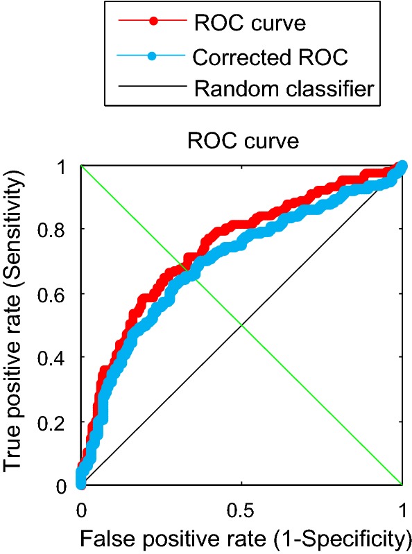
Corrected ROC curve, after decorrelating markers of arousal

The conjunctive analysis did not indicate any effect of frustration on the WMLE. The analysis yielded a value $p\gg 0.1$.

To double check for possible motor confounding factors, EEG data from online trials were visually inspected in the end of each experiment. For instance, subject 3 initially had an accuracy of 100%; however, visual inspection of the EEG signal allowed us to see that the subject consistently produced electromyographic artifacts in the occipital region in the high-WM-load condition. All data were discarded and the subject repeated the experiment on a different day without occipital electrodes. The performance the second time was slightly lower but still well above the chance level (85% correct classification).

Neurophenomenological validation

A total of 92 trials were analysed, with subjects providing the correct answer 82% of the time ($p<0.0001$). Data for individual subjects are summarized in Table 1.

Table 1.

Results of the neurophenomenological validation

Subject	Trials not answered	Noisy trials removed	Total trials analyzed	Correct answers
1	1	1	18	15
2	3	0	17	13
3	0	0	20	17
4	0	0	10	10
5	1	0	19	14
6	7	5	8	6
Total	12	6	92	75 (82%, $p<0.0001$, see “Appendix 4: Estimation of statistical significance” section)

Percentage of correct answers, per subject, to the question to assess whether the feedback was sham or real. Artifacted trials and trials where subjects did not answer were not considered

Temporal behaviour of the WMLE

Half of the subjects had a very stable WMLE. Figure 6 shows the average over the 20 trials of one of these subjects during Task 2. One observes that systematically the WMLE begins to decrease after 10 s. It is important to remember that during the first 8.5 s, the subjects performed mental arithmetic. Afterwards, following a visual cue the subjects stopped the mental arithmetic.

Fig. 6.

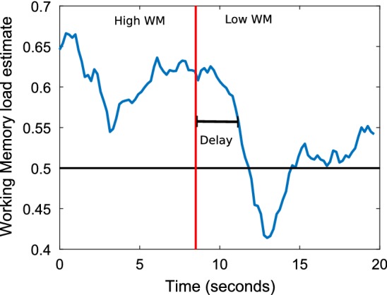
Average over trials of the WMLE time evolution of a typical “good” subject. The first 2.5 s are not a reliable estimation, as the buffer requires 2.5 to be filled. The first 2.5 s of feedback were not displayed to the user

The observed behaviour is consistent with the WM-load switch expected at 8.5 s, plus the BCI delay. The length of such delay is less than 2.5 s, as the WMLE at time $t_0$ considers all the EEG activity that took place between $t_0-2.5$ and $t_0$. After reaching the lowest value, the WMLE systematically increases again, this time possibly due to the feedback information being processed by the subject. Subjects at this point were still processing information, while performing the comparison between the WMLE and their subjectively estimated WM load. Indeed, the new values are relatively high, however not as high as in the first part of the task.

For the other half of the subjects, the behaviour was not as stable across trials, and averages across trials were flattened, suggesting no systematic behaviour. Nevertheless, even for these subjects there was a high rate of correct answers, which means that the WMLE matched successfully their subjective perception of WM load.

The EEG biomarkers: spectral changes in EEG due to WM load

After ensuring the reliable single-trial estimation of WM load, it is useful to go back to the question of what changes are induced in the brain due to WM activity.

For a visual representation of these changes (and not for real-time feedback), we can afford windows of 10 s, instead of the 2.5 s used for the real-time feedback. Shorter windows are useful for a low-latency system, while larger windows allow a more accurate spectral decomposition of the signal.

The power at a certain band for a given channel is a potential biomarker. We computed the grand average across trials and across subjects for each biomarker. Changes across conditions of this grand average are displayed in Fig. 7, using all artifact-free trials. The red colour corresponds to biomarkers that had on average higher values in the high-WM condition, whereas the blue colour corresponds to biomarkers whose average values were lower in the high-WM-load condition. We only used biomarkers conveying useful information for WM prediction.

Fig. 7.

Mean difference between high and low-WM-load conditions for relevant biomarkers. In light, values typically higher in high-WM-load condition. In dark, values typically lower in high-WM-load condition

Due to our multivariable approach, we are not interested in biomarkers that are statistically different across conditions (see the discussion section for more details on why this might not be informative). Instead, we are interested in biomarkers that, when combined, produce patterns that can be identified as typical low-WM or typical high-WM activity.

To determine how many biomarkers are relevant, we ranked them with the Orthogonal Forward Regression feature (in this work feature will be used interchangeably with EEG biomarker) selection technique (see “Offline study: designing the BCI” section) and added them to the model one by one until performance decreased or did not increase significantly.

The biomarkers that were the best predictors of WM load were the following:

• Relative lower beta power, electrode Fp1

• Relative lower beta power, electrode Cz

• Lower gamma power*, electrode Fp1

• Relative upper beta power, electrode Cz

• Alpha power, electrode Oz

• Alpha power*, electrode CP5

Biomarkers with a star (*) increased with increasing WM load, while the others decreased with increasing WM load.

Discussion

We developed a cognitive BCI targeting real-time estimation of working memory load. We validated this model and obtained satisfactory online results. In addition we controlled the model for potential cognitive and motor confounders, and compared the model output with subjective WM-load estimates of the BCI users. 126 trials were used for online BCI validation and 92 trials were used for neurophenomenological validation.

The experiments were designed in success/failure terms for both the online BCI validation and the neurophenomenological validation. Success meant the system correctly predicting the WM-load imposed to the subject in the online BCI validation, and subjects correctly identifying real or sham feedback in the neurophenomenological validation. This dichotomy allowed us to easily assess the statistical significance in terms of binomial trials (“Appendix 4: Estimation of statistical significance” section). Even intuitively it is reasonable to believe that answering correctly 82% of 92 questions (neurophenomenological validation) can hardly occur by chance. To further strengthen the argument of statistical significance, the BCI online validation was assessed with random features in order to estimate the probability of obtaining an AUC of 0.78 or higher by chance. None of the 50,000 iterations with random features yielded such AUC value.

The successful neurophenomenological (Varela 1996) validation is indeed one of the main features of this study. Experimenting with human subjects provides us with the unique possibility of establishing links between subjective states and objective measures (Lutz 2002). These links can be meaningfully validated by the subject only under appropriate experimental conditions. It is required, first, to design an adequate online protocol, and second, to perform careful control tests.

We expect our phenomenological validation to encourage researchers interested in rigorous cognitive monitoring and neurofeedback. Narrowing down the gap between the subjective world and objective measures opens the door to new theoretical approaches and practical implementations. The p value reported in Table 1 is the p value associated to the ensemble of 92 trials because there is no mathematical advantage of computing p values per subject: these results should be reproducible across subjects, which is more interesting than a subject-wise analysis. In addition, with recording sessions of 2–3 h, collecting enough data for every subject to achieve statistical significance would imply recording in different days. Due to the lack of EEG stationarity and the need of re-calibrating the system, the results would no longer be comparable across sessions in any case.

The statistical analysis of the confounders suggests independence between the EEG biomarkers and the tested potential confounders. This holds true even for cognitive confounders necessarily correlated to WM, like the attentional filters or the phonological loop.

The original WM model from Baddeley (Baddeley 1992) considers the phonological loop as a core element of WM, and the embedded-processes model of WM (Cowan 1999) explicitly refers to attentional filters. This independence is a satisfactory result for real-world testing, given that these confounders, being part of WM under certain models, are necessary but not sufficient for an activity to be demanding for WM.

There are several studies on EEG-based WM load estimation; however, to the best of our knowledge, none of them has all the properties required for a real-world, real-time continuous monitoring system. Continuous meaning here that the users validated the dynamical behaviour of the feedback gauge (refreshed at intervals of 150 ms), and not only whether the system predicted the imposed load at the end of the trial.

Studies (Jensen and Tesche 2002; Sauseng et al. 2005a, b), describing statistical differences of biomarkers across WM conditions, aim to make general claims about the neural correlates of WM. Nevertheless, statistically significant differences across conditions are not necessarily sufficient for single-trial classification. Jensen et al. (2002), for instance, report theta activity in frontal areas due to WM activity. However, their further examination highlighted that the theta activity revealed by the grand average was the result of the contribution of a single subject.

Some studies perform single-trial classification (Khasnobish et al. 2017), which is a necessary condition for a system to work online. Nevertheless, many of them (Gevins et al. 1998; Zarjam et al. 2011) are offline.

Neurofeedback online (real-time) experiments have different advantages: from neurophenomenological validation to overfitting prevention. Only online is it possible for subjects to validate in a continuous manner that the feedback is indeed reflecting their instantaneous cognitive state, precisely due to our WM limitations. In general, online approaches allow experimenters to interactively re-design experiments until conclusive hypothesis are attained (Sanchez et al. 2014).

Regarding overfitting, an overfitted model will learn noise and artificially explain events a posteriori, while being unable to predict new events. The analysis of brain signals might involve complex models with many parameters and variables. For these models, there is a high risk of overfitting. A classifier with good online performance ensures that no positive results come from overfitting, as testing data are acquired on the fly.

Other studies (Erdogmus et al. 2005; Grimes et al. 2008; Haapalainen et al. 2010; Heger et al. 2010) describe implementations that are sufficiently fast to work in real-time; however, no actual real-time testing was performed. These are useful feasibility studies, however an online validation would be necessary to evaluate the prototype reliability.

While studies performed online are indeed an important step towards a practical implementation of BCIs, there is still significant room for improvement and potential confounders must be controlled for. Wilson and Russell (2003) train their system with EEG data from subjects performing the NASA Multi-Attribute Task Battery (Comstock Jr and Arnegard 1992). The task has a motor component (manipulating a joystick and a mouse), and different cognitive load levels are imposed by changing the number of events. Hence, with an imbalance of motor activity across conditions, there is a high risk of motor confounding factors being learned by the system. It is not clear then if they are measuring cognitive load or motor activity. The same issue applies to the study by Berka et al. (2004).

The system developed by Kohlmorgen et al. (2007) seems to have balanced motor components; however, there is no cross task. The training session and the application session involved the same type of tasks. It is not clear then whether their results are WM general or task-specific. It has been shown (Baldwin and Penaranda 2012) that accuracies can drop to chance levels when trying to classify workload using a testing task different than the learning one, even if both address the same cognitive function. The latter meaning that the system had learned particularities of the task instead of generalities of the underlying cognitive system.

None of these studies specifically disentangle potential confounding factors, and furthermore, none of them performed neurophenomenological validation.

Besides the methodological aspects, there are two factors, at the level of design, which could explain the success of our prototype. The training task was defined in such a way that the three functions involved in WM (storing, processing and refreshing) were at full capacity in the high-WM-load condition. This might be the reason behind the good generalizability to a different task. On the other hand, adding noisy copies of subjects’ individual data (“Offline study: designing the BCI” section) allows us to deal with a necessary compromise when facing large inter-subject variability: a trade-off between performance and the need to measure strictly WM activity, irrespective of subject idiosyncrasies.

Training the classifier only with the data from the current subject might perform well, but there is a risk that what is measured in the end is not WM. On the other hand, assigning an equal weight to all subjects would only detect changes that are common to all of them, minimising inter-subject differences. Evidently, not all brains respond in the same way, and we are dealing with this variability in a robust way. As an example, Grimes et al. (2008) found that alpha activity increases with memory load for some subjects, while it decreases for others. This is an important remark given that, as mentioned in the introduction, alpha activity is thought of as a potential signature of WM. Addressing this trade-off allows us to build a BCI adapted to the user, while ensuring that a general underlying cognitive function is measured. By adding noisy copies we are also making the classifier more robust to noise.

Aiming at generalizability, an additional source of variability was imposed in Task 2. Subjects were able to choose what kind of arithmetic operations to do. In spite of this imposed variability, subjects consistently identified the feedback provided as their actual cognitive load whenever it was the case. Conversely, they correctly identified the sham feedback as such.

The results of the neurophenomenological validation, although positive, could be a conservative estimation, as, even when using a functional WM-BCI, subjects might fail at the neurophenomenological validation. The reason is that introducing the feedback gauge and asking subjects for neurophenomenological validation imposes an additional WM load that cannot be neglected.

Besides the intrinsic WM load imposed by the task, the neurophenomenological validation adds three additional sources of WM load. The first source arises from the fact that subjects are required to estimate their own WM load, which imposes and additional load due to introspection. In addition, subjects need to compare their load estimation with the feedback provided, making a binary judgement: correct or incorrect feedback. Furthermore, as we analyse EEG epochs of 2.5 s, our estimate is delayed. Subjects therefore need to compare the current feedback with the WM load they experienced a few instants ago. This comparison is the second source of WM load.

All the steps describe above are repeated at different instants during the trial, and all the partial binary judgements are stored so that the subject can provide a global decision at the end of the trial. Storing the binary decisions is the third additional source of WM load.

As Lutz and Thompson (2003) point out, generating first-person reports about an experience can modify that experience itself. Due to the additional cognitive resources required, subjects were given 6 trials to become familiar with the procedure. After these 6 trials, one of the subjects expressed feeling unable to perform the task and did not continue. The subject explained that the information to be processed was overwhelming. Another subject, subject 6 in the table of “Neurophenomenological validation” section, expressed difficulties providing an answer due to this same situation. The latter is reflected in the relatively high number of unanswered questions of this particular subject.

These testimonies suggest that results in Table 1 could be a conservative estimate of the BCI performancee: subjects required a certain degree of skills and training to perform the neurophenomenological validation, and before reaching an adequate level of expertise their answers are error-prone. This task is more demanding than a classical mental calculation task, which only requires intrinsic task load. In fact, the latter was the reason why we compared mental computation vs. “rest”, because the rest condition was not rest indeed. Although the mental arithmetic had stopped, subjects still had to devote cognitive resources to perform the task. However, despite this additional WM load not necessary in the real-life counterpart of the experiment, once the BCI is validated by enough subjects to achieve significance, we can hypothesise that it is usable for all literate subjects (subjects with an adequate performance in the BCI validation), regardless of individual results of the neurophenomenological validation.

In other words, literate subjects who cannot perform the neurophenomenological validation may still be able to use the BCI in a real-world task, in which they are expected to believe the feedback, not to rate it. In an adaptive system, users might not even receive any feedback, as the feedback could be used for the system to trigger an action (lower the task difficulty, start an autopilot, etc.).

The choice of a reversed gauge as sham feedback was to preserve the dynamic behaviour of the feedback. Had we presented, for instance, random feedback, subjects could have learned, depending on the underlying distribution and dynamics, that random motion of the bar implies sham feedback. In addition, the choice of a disappearing cue in Task 2 imposed a time-locked change in the WM load, helping subjects handling delays of the BCI.

Regarding the WMLE, given that no previous studies had been done performing neurophenomenological validation, the dynamics of the WM load remained an open question.

Of our six online subjects doing the cross task, two mentioned that it was the dynamics of the feedback gauge in particular that helped them decide whether it was sham or real. In other words, the most informative event for them was whether the gauge increased or decreased at key moments, rather than the absolute value of the gauge. For another two, it was both the absolute value and the dynamics; they indeed mentioned that it was extremely easy to know when it was real or sham. For the remaining two, there was no clear distinction.

Generally speaking, they all stated that the (true) feedback was a measure of their WM load, which in turn was reflected in the high rate of correct answers of the neurophenomenological validation. Furthermore, most of them mentioned spontaneously that it was clear that the sham feedback signal was the reverse of their WM load. This information was not disclosed to them in advance, and supports the claim that the feedback gauge contains WM-load information. Had it been noise (not WM related), users would be unable to distinguish the real and the reversed gauge. Indeed, at a first glance, it might look like the choice of a reversed gauge as sham induces some bias making the task of deciding real or sham easier. However, a reversed gauge only simplifies the task if the WMLE is not noise, as the reverse of noise is still noise.

As mentioned in the above paragraph, adding noise to the real feedback to make it sham would artificially create two dynamically distinct behaviours even if the WMLE does not convey information about WM load, and hence it was avoided.

Although the global mean of the WMLE remained lower for the low-WM-load condition than for the high-WM-load condition, there were peaks of the WMLE in both conditions. Further investigation needs to be carried out to determine whether these peaks correspond to refreshing, peaks of processing, or simply noise. One subject spontaneously reported that these corresponded to peaks of processing; however, this was not reported by the other subjects. This is not surprising, as subjects in general are not used to monitoring their WM and to thinking of it in terms of its subprocesses.

Expertise and knowledge of the subprocesses of WM would be required to answer that question, and the above-mentioned subject had some prior knowledge about WM.

It is of theoretical relevance to investigate which aspects of WM induce more load in the central executive and how these events are temporally distributed depending on the WM load. In addition, if these peaks represent true activity and not noise, then they could be used to improve the performance of the BCI as well.

Some of the training trials of the low condition will happen to contain these peaks, despite the fact that the subject is engaged in the low-WM-load condition. Peaks in the low-WM-load condition could be present for different reasons. The subject could have been temporarily allocating mental resources to non-task related activities: attending to external stimuli, mind-wandering due to lack of motivation, etc. In other words, we cannot impose a specific, constant WM load. Moreover, if peaks are refreshing events, for example, they occur as well in the low-WM-load condition, perhaps at a different rate and/or different intensity, but they do occur.

That being said, if we have an objective measurement (the WMLE), we could iteratively improve the quality of our offline database. For instance, by reallocating peaks in the low-WM-load condition to the other class (high-WM load), run the algorithm again, and repeat until stability is reached (the size of both classes remains constant), or alternatively until another stopping criterion is met, in the absence of stability. In fact, theses peaks of activity in the low-WM condition might be the reason the performance of the neurophenomenological validation seems better than the BCI validation. Neurophenomenological validation shows the prediction in real time. If low-WM-load trials are contaminated with high-WM-load activity (label noise), the subject might know, and perform an adequate validation still. On the other hand, the label (low WM or high WM) remains constant throughout the whole trail regardless of the subject’s state, and the BCI validation performance considers the label, rather than the internal state of the subject, as truth.

As for the biomarkers themselves, we observe different markers whose joint activity predicts WM load (Fig. 7). Instead of using single biomarkers to estimate WM load, we derived composite biomarkers from weighted combinations of several biomarkers. Such an estimate is more reliable, and more realistic considering that WM is a complex cognitive function involving the coordination of several brain areas. We are therefore associating patterns of joint activity to WM conditions. Some of these biomarkers are consistent with the literature, like the decrease in the alpha power at occipital regions mentioned in the introduction. However, it is important to stress again that considering them as isolated markers of WM activity might be misleading. Conversely, there were also biomarkers whose change across WM conditions was statistically significant; however, including them in the analysis decreased the ability of the BCI to correctly estimate WM load.

One potential explanation is that these changes are due to subject variability and not to a fundamental aspect of WM. The above-mentioned study (Jensen et al. 2002) in which the grand average showed significant changes in the theta power because of the contribution of one single subject is an example. Incidentally, we did not find any significant changes in the theta range. Another explanation is multiple hypothesis testing. If we test hundreds of biomarkers, some of them will, by chance, appear statistically significant, even if there is no real correlation. This illustrates how multivariable classification techniques can be powerful techniques for making inferences. Even though some changes across both conditions would appear as statistically significant, their lack of generality renders them useless for prediction. We therefore have a simple yet powerful criterion: if, by adding information (biomarkers), our ability to classify decreases, then it is not relevant information, even though it seems statistically significant. Besides, combining several biomarkers into a single score (the WMLE) reduces the risks associated with multiple hypothesis testing.

A situation in between might occur. Adding biomarkers could neither increase nor decrease the classification power. One potential explanation is that these biomarkers are highly correlated with previously selected biomarkers. Therefore, our list of relevant biomarkers is by no means extensive, as mentioned in “The EEG biomarkers: spectral changes in EEG due to WM load” section.

Biomarkers redundant to the selected ones were not chosen, and this could be the reason for the apparent asymmetry in Fig. 7. In fact, running the code with different parameters would lead sometimes to the selection of the symmetric electrode, for instance, electrode CP6 instead of electrode CP5. Moreover, biomarkers that do not increase the classification power may increase it by using more sophisticated techniques, such as support vector machines or neural networks, that better capture the complexity of the underlying system. The latter is further developed at the end of the discussion.

Despite the multivariate approach, our approach nonetheless is far from conveying a global view.

EEG consists of a few scalp recordings of the activity of a very complex underlying system. Acknowledging our relatively short (for a multivariable analysis) database, aiming at robustness and as a first attempt, we chose a linear feature-selection technique and a linear classifier. A linear feature-selection technique might not necessarily work when correlations between features and the output are not linear. A linear classifier assumes a certain topology in the feature space: classes can be separated with a line, plane or hyperplane. A larger dataset would allow the use of feature-selection techniques and classifiers that better capture the underlying complexity. In addition, we are ignoring potential neural mechanisms that could be active when subjects stay at the limit of their WM capacity for a long period of time. If such mechanisms exist, the distribution of biomarkers in the feature space could be completely different.

A real-world application should thus explore to what extent WM-load-detection protocols might need to be modified when high WM load is imposed for long periods of time.

Appendix 1: Images used for Task 1

Figures used to determine the memory span

Geometric Shapes	Fruits	Landscape
Circle	Apple	House
Pentagon	Banana	Building
Square	Orange	Church
Rhombus	Pear	Castle
Cross	Grape	Bridge
Star	Watermelon	Tower
Triangle	Pineapple	Tree

Figures used for the test

Animals	Vehicles	Supplies	Clothes
Cat	Plane	Book	Trousers
Deer	Train	Scissors	Shirt
Dog	Skateboard	Pen	Hat
Elephant	Truck	Ruler	Shoes
Penguin	Car	Backpack	Socks
Snake	Ship	Compass	Belt
Turtle	Bicycle	Set square	Tie

Appendix 2: Technical aspects of the BCI system

Offline study: designing the BCI

The offline study was a feasibility study, in which the constrains that would be encountered online were taken into account and reproduced. Examples of the online constraints include low latency of the online system (and therefore only a low number of features can be afforded for a quick analysis), limited calibration data for short calibration sessions, and the inability to remove artifacts such as eye-blinks. We called these parameters $P_1,P_2,P_3,\dots$, and an acceptable range of each of them was determined. For different combinations of the acceptable parameters, the following pipeline was performed:

1. 20 subjects performed Task 1 while wearing the EEG set. Frequencies below 1 Hz and above 45 Hz were removed from the EEG signal with a 3rd order Butterworth filter. The EEG data were segmented into epochs of $P_1$ seconds.

2. A subject $s_i$ was removed from the dataset. The data of subject $s_i$ were divided into two subsets, one subset with $P_2$ epochs that will simulate the calibration session (“Online tests: the calibration session” section), and another subset with the remaining epochs. The calibration data and the data from the remaining subjects were used as training data. The data from the subject that were not part of the calibration data were used as testing data.

3. For the training data, each epoch was visually inspected and all the epochs contaminated with noise or muscular artifacts were rejected. In particular, epochs with eye-blinks or with arousal flags were rejected. An arousal flag was placed on an epoch if ether a distracter or the target was displayed during its course. During preliminary tests, subjects had reported an arousal effect due to the appearance of distracters or targets. The testing data were not cleaned.

4. For both the training and the testing data, spectral features were extracted using the Matlab p-Welch function, with a Hamming window of 0.5 s. The spectral features were absolute and relative power in the following bands: delta (1–4 Hz), theta (4–8 Hz), alpha (8–12 Hz), lower beta (12–20 Hz), upper beta (20–30 Hz) and lower gamma (30–45 Hz). The relative power in a band is the fraction of the total power in that band. The latter being normalised has the advantage of reducing inter-subject variability. Having 16 channels, 2 features per band, and 6 bands, we obtained 192 features for each epoch.

5. The calibration data were expanded by adding noisy copies. Enough noisy copies were created so that the number of epochs of the expanded calibration data divided by the number of epochs of the total training dataset equalled $P_3$. The noise added was Gaussian noise with zero mean and standard deviation equal to $P_4$ times the standard deviation of the feature.

6. To select relevant features, orthogonal forward regression (OFR) (Stoppiglia et al. 2003) was performed on the above matrix, the best $P_5$ features were kept. OFR is a linear regression technique that can be used as a supervised feature selection technique. In the first step of OFR, features are ranked in order of decreasing correlation to the classifier output; the first selected feature is the top-ranking feature. In the second step, all remaining features, and the output, are orthogonalized with respect to the first selected feature, thereby discarding the part of the output that was explained by that feature; the projected features are ranked in order of decreasing correlation to the projected output, and the top-ranking feature is selected. Orthogonalization, ranking and selection are iterated until $P_5$ features are selected. OFR was used instead of other common procedures such as Common Spatial Pattern (CSP) (Koles et al. 1990; Cheng et al. 2017) in order to minimise the number of required sensors for future implementations. In addition, the weighted average of features from different sensors is similar to the spatial average provided by CSP.

7. A linear discriminant analysis [LDA (Fisher 1936)] classifier was trained with the selected features and their corresponding labels (high or low-WM load). The output of the classifier is the posterior probability that the EEG segment belongs to the high-WM-load condition. A typically high-WM-load segment then would have a high posterior probability, therefore we defined the WMLE as the posterior probability.

8. We performed cross-validation by iterating over all possible subjects $s_i$ for a given set of possible parameters ($P_1$, $P_2$, $P_3$, $P_4$, $P_5$), the performance of the classifier measured as the AUC was computed as a function of said parameters. The set of parameters that maximised the performance of the classifier was chosen, in other words, the parameters were optimised by cross-validation. Cross-validation is a family of techniques to asses a model’s ability to generalise when faced with new data, in this case, the testing data that were removed from the dataset. The reader interested in the topic can consult (Kohavi 1995) for a more in-depth discussion.

The set of parameters that represented the best trade-off between classification performance and feasibility was chosen to build the actual BCI. The values are shown in Table 2.

Table 2.

Parameters that maximise the performance of the classifier

Parameter	Description	Value
1	Epoch length	2.5 s
2	Calibration epochs	45 per class
3	Subject weight	0.65
4	Noise level	1.5
5	Number of features	8

It is important to notice that although optimising by cross-validation might overestimate the performance results, we did this only to design the classifier, and all the results presented in this work are online results. Online there was no hypothesis testing (parameter selection), therefore, as the BCI design (set of parameters) was fixed for the online tests, p value corrections are not necessary. Furthermore, even though the number of features was optimised by cross-validation, the set of features itself (step 6) was chosen inside every cross-validation fold (step 8).

Online analysis: from EEG recordings to a WMLE

The online experiments followed the procedure outlined in the previous section. As before, recordings started with a calibration session, calibration data were cleaned and then added to the cleaned data from the 20 subjects recorded offline. This time however the set of parameters ($P_1$, $P_2$, $P_3$, $P_4$, $P_5$) was already set, and the pipeline described in the previous section was performed with the values of the Table 2.

Figure 8 shows how the information from the previous section (offline study) is integrated with that in this section (calibration) to select a good set of features and train the classifier that was designed offline.

Fig. 8.

Design methodology

Afterwards, the BCI is able to provide a WMLE. A continuous stream of data is analysed. A sliding window including the last 2.5 s of EEG is used as input.

Appendix 3: Arithmetic operations in Task 2

A random sequence of digits $d_1,d_2,\dots ,d_n$ was presented to the subjects in each trial. Three possible ways of manipulating the digits were suggested to the subjects, who were asked to choose the one that felt more resource demanding for them:

• Progressive multiplication. Multiply $d_1{d}_2\dots d_i$ until time is over

• Pairwise multiplication and successive addition. Multiply $d_1$ and $d_2$ and store the result. Add the result to the product of $d_3$ and $d_4$, replace the result. Add the result to the product of $d_5$ and $d_6$, replace the result. Continue until time is over.

• Free choice. Subjects comfortable with their arithmetic skills were left to choose the structure of the operations, provided they maintained a high level of use of their mental resources.

Appendix 4: Estimation of statistical significance

We developed a method to estimate analytically the statistical significance of the performance of a two-class classifier. The null hypothesis is that the results come from a random classifier, whereas the alternative hypothesis is that the classifier is based on informative features. The first step towards estimating significance, then, is to choose a random classifier and to determine its success rate. Let us assume that our dataset consists of N examples, with $N_1$ examples of class 1 and $N-N_1$ examples of class 2, with $N_1\ge N/2$. The best that a random classifier can do is to take into account the prior probabilities of the classes. Denoting by q the prior probability of class 1, assumed to be larger than 0.5, and estimated by $N_1/N$, a possible random classification rule is to assign any object to class 1 with probability q. The probability of correct classification of this classifier (which can be estimated by its rate of correct classification) is given by : $c_0=q^2+{(1-q)}^2$. Let us define a random variable whose realisation $z_i$, for example i, is

$$\begin{array}{c}\hfill z_i=\left\{\begin{array}{cc}1\hfill & \text{if the random classifier classified example}i\text{correctly}\hfill \\ 0\hfill & \text{otherwise}\hfill \end{array}\right)\end{array}$$

The total number of successes, $Z={\sum }_{i=1}^N{z}_i$, follows a binomial distribution $Z\sim B(N,c_0)$, and hence the probability of obtaining exactly k successes is

$$\begin{array}{c}\hfill Pr(Z=k)=\left(\begin{array}{c}N\\ k\end{array}\right)c_0^k{(1-c_0)}^{N-k}\end{array}$$

The p value is, by definition, the probability of obtaining results at least as extreme as the observed ones, assuming that the null hypothesis is true. Our goal is to compare a random classifier with a particular classifier that yielded c correct answers. In this case, “results as extreme” means observing at least c correct answers in a random classifier. Therefore, the p value associated with the null hypothesis defined above can be computed as

$$\begin{array}{c}\hfill p=\sum _{k=c}^{N}Pr(Z=k)\end{array}$$

In general, the use of any other random classifier would lead to a different $c_0$. In particular, the most efficient classification rule under complete lack of informative predictors is the zero classifier, that assigns all the objects to the largest class. In the above notation, the rate of correct classification of a zero classifier is $c_{0z}=q$. As, by definition, $0.5<q<1$, it is easy to show that $c_{0z}>c_0$ for all q. However, although the zero classifier is the best classification rule when no relevant predictors are available, for a zero classifier $Pr(Z=k)=0$ if $k\ne N_1$ (by definition a zero classifier can correctly predict only $N_1$ objects). Therefore, for any classifier with a number of correct predictions larger than $N_1$, p would be zero. It is a good practice to compare classification results with those of a zero classifier when facing imbalanced datasets. However, a zero classifier is not useful for computing p values.

Funding

This work was supported by a Consejo Nacional de Ciencia y Tecnología (Mexican government) grant (to A.M.-S.).

References

- Allison BZ, Neuper C. Could anyone use a BCI? In: Tan D, Nijholt A, editors. Brain–computer interfaces. Berlin: Springer; 2010. pp. 35–54. [Google Scholar]
- Antonenko P, Paas F, Grabner R, Van Gog T. Using electroencephalography to measure cognitive load. Educ Psychol Rev. 2010;22(4):425–438. doi: 10.1007/s10648-010-9130-y. [DOI] [Google Scholar]
- Awh E, Vogel EK, Oh S-H. Interactions between attention and working memory. Neuroscience. 2006;139(1):201–208. doi: 10.1016/j.neuroscience.2005.08.023. [DOI] [PubMed] [Google Scholar]
- Baddeley A. Working memory. Science. 1992;255(5044):556–559. doi: 10.1126/science.1736359. [DOI] [PubMed] [Google Scholar]
- Baddeley A. Working memory: looking back and looking forward. Nat Rev Neurosci. 2003;4(10):829–839. doi: 10.1038/nrn1201. [DOI] [PubMed] [Google Scholar]
- Baddeley AD (2017) The concept of working memory: a view of its current state and probable future development. In: Exploring working memory. Routledge, Abingdon, pp 99–106 [DOI] [PubMed]
- Baldwin CL, Penaranda B. Adaptive training using an artificial neural network and EEG metrics for within-and cross-task workload classification. NeuroImage. 2012;59(1):48–56. doi: 10.1016/j.neuroimage.2011.07.047. [DOI] [PubMed] [Google Scholar]
- Berka C, Levendowski DJ, Cvetinovic MM, Petrovic MM, Davis G, Lumicao MN, Zivkovic VT, Popovic MV, Olmstead R. Real-time analysis of EEG indexes of alertness, cognition, and memory acquired with a wireless EEG headset. Int J Hum-Comput Interact. 2004;17(2):151–170. doi: 10.1207/s15327590ijhc1702_3. [DOI] [Google Scholar]
- Borghini G, Astolfi L, Vecchiato G, Mattia D, Babiloni F. Measuring neurophysiological signals in aircraft pilots and car drivers for the assessment of mental workload, fatigue and drowsiness. Neurosci Biobehav Rev. 2014;44:58–75. doi: 10.1016/j.neubiorev.2012.10.003. [DOI] [PubMed] [Google Scholar]
- Cavanagh JF, Frank MJ. Frontal theta as a mechanism for cognitive control. Trends Cogn Sci. 2014;18(8):414–421. doi: 10.1016/j.tics.2014.04.012. [DOI] [PMC free article] [PubMed] [Google Scholar]
- Cheney W, Kincaid D. Linear algebra: theory and applications. Canberra: The Australian Mathematical Society; 2009. p. 110. [Google Scholar]
- Cheng M, Lu Z, Wang H. Regularized common spatial patterns with subject-to-subject transfer of EEG signals. Cogn Neurodyn. 2017;11(2):173–181. doi: 10.1007/s11571-016-9417-x. [DOI] [PMC free article] [PubMed] [Google Scholar]
- Comstock Jr JR, Arnegard RJ (1992) The multi-attribute task battery for human operator workload and strategic behavior research
- Cowan N. An embedded-processes model of working memory. In: Miyake A, Shah P, editors. Models of working memory: mechanisms of active maintenance and executive control. Cambridge: Cambridge University Press; 1999. p. 506. [Google Scholar]
- Cragg L, Richardson S, Hubber PJ, Keeble S, Gilmore C. When is working memory important for arithmetic? The impact of strategy and age. PLoS ONE. 2017;12(12):e0188693. doi: 10.1371/journal.pone.0188693. [DOI] [PMC free article] [PubMed] [Google Scholar]
- de Fockert JW, Rees G, Frith CD, Lavie N. The role of working memory in visual selective attention. Science. 2001;291(5509):1803–1806. doi: 10.1126/science.1056496. [DOI] [PubMed] [Google Scholar]
- Dehais F, Duprès A, Blum S, Drougard N, Scannella S, Roy RN, Lotte F. Monitoring pilot’s mental workload using ERPs and spectral power with a six-dry-electrode EEG system in real flight conditions. Sensors. 2019;19(6):1324. doi: 10.3390/s19061324. [DOI] [PMC free article] [PubMed] [Google Scholar]
- Di Flumeri G, Borghini G, Aricò P, Sciaraffa N, Lanzi P, Pozzi S, Vignali V, Lantieri C, Bichicchi A, Simone A, et al. EEG-based mental workload neurometric to evaluate the impact of different traffic and road conditions in real driving settings. Front Hum Neurosci. 2018;12:509. doi: 10.3389/fnhum.2018.00509. [DOI] [PMC free article] [PubMed] [Google Scholar]
- Downing PE. Interactions between visual working memory and selective attention. Psychol Sci. 2000;11(6):467–473. doi: 10.1111/1467-9280.00290. [DOI] [PubMed] [Google Scholar]
- Erdogmus D, Adami A, Pavel M, Lan T, Mathan S, Whitlow S, Dorneich M (2005) Cognitive state estimation based on EEG for augmented cognition. In: Conference proceedings. 2nd international IEEE EMBS conference on neural engineering, 2005. IEEE, pp 566–569
- Ericsson KA, Delaney PF. Working memory in everyday skilled performance. In: Miyake A, Shah P, editors. Models of working memory: mechanisms of active maintenance and executive control. Cambridge: Cambridge University Press; 1999. p. 274. [Google Scholar]
- Farwell LA, Donchin E. Talking off the top of your head: toward a mental prosthesis utilizing event-related brain potentials. Electroencephalogr Clin Neurophysiol. 1988;70(6):510–523. doi: 10.1016/0013-4694(88)90149-6. [DOI] [PubMed] [Google Scholar]
- Fisher RA. The use of multiple measurements in taxonomic problems. Ann Eugen. 1936;7(2):179–188. doi: 10.1111/j.1469-1809.1936.tb02137.x. [DOI] [Google Scholar]
- Gaume A, Vialatte A, Mora-Sánchez A, Ramdani C, Vialatte F. A psychoengineering paradigm for the neurocognitive mechanisms of biofeedback and neurofeedback. Neurosci Biobehav Rev. 2016;68:891–910. doi: 10.1016/j.neubiorev.2016.06.012. [DOI] [PubMed] [Google Scholar]
- Gaume A, Dreyfus G, Vialatte F-B. A cognitive brain–computer interface monitoring sustained attentional variations during a continuous task. Cogn Neurodyn. 2019;13(3):257–269. doi: 10.1007/s11571-019-09521-4. [DOI] [PMC free article] [PubMed] [Google Scholar]
- Gerjets P, Walter C, Rosenstiel W, Bogdan M, Zander TO. Cognitive state monitoring and the design of adaptive instruction in digital environments: lessons learned from cognitive workload assessment using a passive brain–computer interface approach. Front Neurosci. 2014;8(2014):385. doi: 10.3389/fnins.2014.00385. [DOI] [PMC free article] [PubMed] [Google Scholar]
- Gevins A, Smith ME, Leong H, McEvoy L, Whitfield S, Du R, Rush G. Monitoring working memory load during computer-based tasks with EEG pattern recognition methods. Hum Factors J Hum Factors Ergon Soc. 1998;40(1):79–91. doi: 10.1518/001872098779480578. [DOI] [PubMed] [Google Scholar]
- Grimes D, Tan DS, Hudson SE, Shenoy P, Rao RP (2008) Feasibility and pragmatics of classifying working memory load with an electroencephalograph. In: Proceedings of the SIGCHI conference on human factors in computing systems. ACM, New York, pp 835–844
- Haapalainen E, Kim S, Forlizzi JF, Dey AK (2010) Psycho-physiological measures for assessing cognitive load. In: Proceedings of the 12th ACM international conference on Ubiquitous computing. ACM, New York, pp 301–310
- Haenschel C, Baldeweg T, Croft RJ, Whittington M, Gruzelier J. Gamma and beta frequency oscillations in response to novel auditory stimuli: a comparison of human electroencephalogram (EEG) data with in vitro models. Proc Natl Acad Sci. 2000;97(13):7645–7650. doi: 10.1073/pnas.120162397. [DOI] [PMC free article] [PubMed] [Google Scholar]
- Hart SG, Staveland LE. Development of NASA-TLX (task load index): results of empirical and theoretical research. Adv Psychol. 1988;52:139–183. doi: 10.1016/S0166-4115(08)62386-9. [DOI] [Google Scholar]
- Heger D, Putze F, Schultz T (2010) Online workload recognition from EEG data during cognitive tests and human–machine interaction. In: Annual conference on artificial intelligence. Springer, Berlin, pp 410–417
- Hinterberger T, Kübler A, Kaiser J, Neumann N, Birbaumer N. A brain–computer interface (BCI) for the locked-in: comparison of different EEG classifications for the thought translation device. Clin Neurophysiol. 2003;114(3):416–425. doi: 10.1016/S1388-2457(02)00411-X. [DOI] [PubMed] [Google Scholar]
- Jensen O, Tesche CD. Frontal theta activity in humans increases with memory load in a working memory task. Eur J Neurosci. 2002;15(8):1395–1399. doi: 10.1046/j.1460-9568.2002.01975.x. [DOI] [PubMed] [Google Scholar]
- Jensen O, Gelfand J, Kounios J, Lisman JE. Oscillations in the alpha band (9–12 Hz) increase with memory load during retention in a short-term memory task. Cereb Cortex. 2002;12(8):877–882. doi: 10.1093/cercor/12.8.877. [DOI] [PubMed] [Google Scholar]
- Khasnobish A, Datta S, Bose R, Tibarewala D, Konar A. Analyzing text recognition from tactually evoked EEG. Cogn Neurodyn. 2017;11(6):501–513. doi: 10.1007/s11571-017-9452-2. [DOI] [PMC free article] [PubMed] [Google Scholar]
- Kintsch W, Patel VL, Ericsson KA. The role of long-term working memory in text comprehension. Psychologia. 1999;42(4):186–198. [Google Scholar]
- Kleiner M, Brainard D, Pelli D, Ingling A, Murray R, Broussard C. What’s new in psychtoolbox-3. Perception. 2007;36(14):1. [Google Scholar]
- Kohavi R, et al. A study of cross-validation and bootstrap for accuracy estimation and model selection. IJCAI. 1995;14:1137–1145. [Google Scholar]
- Kohlmorgen J, Dornhege G, Braun M, Blankertz B, Müller K-R, Curio G, Hagemann K, Bruns A, Schrauf M, Kincses W, et al. Improving human performance in a real operating environment through real-time mental workload detection. In: Dornhege G, Millán JR, Hinterberger T, McFarland D, et al., editors. Toward brain–computer interfacing. Cambridge: MIT Press; 2007. pp. 409–422. [Google Scholar]
- Koles ZJ, Lazar MS, Zhou SZ. Spatial patterns underlying population differences in the background EEG. Brain Topogr. 1990;2(4):275–284. doi: 10.1007/BF01129656. [DOI] [PubMed] [Google Scholar]
- Lotte F, Larrue F, Mühl C. Flaws in current human training protocols for spontaneous brain–computer interfaces: lessons learned from instructional design. Front Hum Neurosci. 2013;7:568. doi: 10.3389/fnhum.2013.00568. [DOI] [PMC free article] [PubMed] [Google Scholar]
- Lutz A. Toward a neurophenomenology as an account of generative passages: a first empirical case study. Phenomenol Cogn Sci. 2002;1(2):133–167. doi: 10.1023/A:1020320221083. [DOI] [Google Scholar]
- Lutz A, Thompson E. Neurophenomenology integrating subjective experience and brain dynamics in the neuroscience of consciousness. J Conscious Stud. 2003;10(9–10):31–52. [Google Scholar]
- Mizuno K, Tanaka M, Yamaguti K, Kajimoto O, Kuratsune H, Watanabe Y. Mental fatigue caused by prolonged cognitive load associated with sympathetic hyperactivity. Behav Brain Funct. 2011;7(1):17. doi: 10.1186/1744-9081-7-17. [DOI] [PMC free article] [PubMed] [Google Scholar]
- Mohanchandra K, Saha S. A communication paradigm using subvocalized speech: translating brain signals into speech. Augment Hum Res. 2016;1(1):3. doi: 10.1007/s41133-016-0001-z. [DOI] [Google Scholar]
- Mora-Sánchez A, Gaume A, Dreyfus G, Vialatte F-B (2015) A cognitive brain–computer interface prototype for the continuous monitoring of visual working memory load. In: 2015 IEEE 25th international workshop on machine learning for signal processing (MLSP). IEEE, pp 1–5
- Mora-Sánchez A, Dreyfus G, Vialatte F-B. Scale-free behaviour and metastable brain-state switching driven by human cognition, an empirical approach. Cogn Neurodyn. 2019;13:1–16. doi: 10.1007/s11571-019-09533-0. [DOI] [PMC free article] [PubMed] [Google Scholar]
- Müller K-R, Tangermann M, Dornhege G, Krauledat M, Curio G, Blankertz B. Machine learning for real-time single-trial EEG-analysis: from brain–computer interfacing to mental state monitoring. J Neurosci Methods. 2008;167(1):82–90. doi: 10.1016/j.jneumeth.2007.09.022. [DOI] [PubMed] [Google Scholar]
- Muller-Putz GR, Pfurtscheller G. Control of an electrical prosthesis with an SSVEP-based BCI. IEEE Trans Biomed Eng. 2008;55(1):361–364. doi: 10.1109/TBME.2007.897815. [DOI] [PubMed] [Google Scholar]
- Mumtaz W, Vuong PL, Xia L, Malik AS, Rashid RBA. An EEG-based machine learning method to screen alcohol use disorder. Cogn Neurodyn. 2017;11(2):161–171. doi: 10.1007/s11571-016-9416-y. [DOI] [PMC free article] [PubMed] [Google Scholar]
- Nasrabadi NM. Pattern recognition and machine learning. J Electron Imaging. 2007;16(4):049901. doi: 10.1117/1.2819119. [DOI] [Google Scholar]
- Paas F, Renkl A, Sweller J. Cognitive load theory and instructional design: recent developments. Educ Psychol. 2003;38(1):1–4. doi: 10.1207/S15326985EP3801_1. [DOI] [Google Scholar]
- Sanchez G, Daunizeau J, Maby E, Bertrand O, Bompas A, Mattout J. Toward a new application of real-time electrophysiology: online optimization of cognitive neurosciences hypothesis testing. Brain Sci. 2014;4(1):49–72. doi: 10.3390/brainsci4010049. [DOI] [PMC free article] [PubMed] [Google Scholar]
- Sauseng P, Klimesch W, Doppelmayr M, Pecherstorfer T, Freunberger R, Hanslmayr S. EEG alpha synchronization and functional coupling during top-down processing in a working memory task. Hum Brain Mapp. 2005;26(2):148–155. doi: 10.1002/hbm.20150. [DOI] [PMC free article] [PubMed] [Google Scholar]
- Sauseng P, Klimesch W, Schabus M, Doppelmayr M. Fronto-parietal EEG coherence in theta and upper alpha reflect central executive functions of working memory. Int J Psychophysiol. 2005;57(2):97–103. doi: 10.1016/j.ijpsycho.2005.03.018. [DOI] [PubMed] [Google Scholar]
- Shorrock ST. Errors of memory in air traffic control. Saf Sci. 2005;43(8):571–588. doi: 10.1016/j.ssci.2005.04.001. [DOI] [Google Scholar]
- Stoppiglia H, Dreyfus G, Dubois R, Oussar Y. Ranking a random feature for variable and feature selection. J Mach Learn Res. 2003;3:1399–1414. [Google Scholar]
- Strijkstra AM, Beersma DG, Drayer B, Halbesma N, Daan S. Subjective sleepiness correlates negatively with global alpha (8–12 Hz) and positively with central frontal theta (4–8 Hz) frequencies in the human resting awake electroencephalogram. Neurosci Lett. 2003;340(1):17–20. doi: 10.1016/S0304-3940(03)00033-8. [DOI] [PubMed] [Google Scholar]
- Sweller J. Cognitive load theory. In: Mestre JP, Ross BH, editors. Psychology of learning and motivation. New-York: Elsevier; 2011. pp. 37–76. [Google Scholar]
- Swets JA. Signal detection theory and ROC analysis in psychology and diagnostics: collected papers. Hove: Psychology Press; 2014. [Google Scholar]
- Tafreshi TF, Daliri MR, Ghodousi M. Functional and effective connectivity based features of EEG signals for object recognition. Cogn Neurodyn. 2019;13(6):555–566. doi: 10.1007/s11571-019-09556-7. [DOI] [PMC free article] [PubMed] [Google Scholar]
- Varela FJ. Neurophenomenology: a methodological remedy for the hard problem. J Conscious Stud. 1996;3(4):330–349. [Google Scholar]
- Varela FJ, Thompson E, Rosch E. The embodied mind: cognitive science and human experience. Cambridge: MIT Press; 2017. [Google Scholar]
- Vialatte F-B, Cichocki A. Split-test Bonferroni correction for QEEG statistical maps. Biol Cybern. 2008;98(4):295–303. doi: 10.1007/s00422-008-0210-8. [DOI] [PubMed] [Google Scholar]
- Vogel EK, McCollough AW, Machizawa MG. Neural measures reveal individual differences in controlling access to working memory. Nature. 2005;438(7067):500–503. doi: 10.1038/nature04171. [DOI] [PubMed] [Google Scholar]
- Wilson GF, Russell CA. Real-time assessment of mental workload using psychophysiological measures and artificial neural networks. Hum Factors J Hum Factors Ergon Soc. 2003;45(4):635–644. doi: 10.1518/hfes.45.4.635.27088. [DOI] [PubMed] [Google Scholar]
- Wolpaw JR, Birbaumer N, Heetderks WJ, McFarland DJ, Peckham PH, Schalk G, Donchin E, Quatrano LA, Robinson CJ, Vaughan TM, et al. Brain–computer interface technology: a review of the first international meeting. IEEE Trans Rehabil Eng. 2000;8(2):164–173. doi: 10.1109/TRE.2000.847807. [DOI] [PubMed] [Google Scholar]
- Zander TO, Kothe C. Towards passive brain–computer interfaces: applying brain–computer interface technology to human–machine systems in general. J Neural Eng. 2011;8(2):025005. doi: 10.1088/1741-2560/8/2/025005. [DOI] [PubMed] [Google Scholar]
- Zarjam P, Epps J, Chen F (2011) Characterizing working memory load using EEG delta activity. In: Signal processing conference, 2011 19th European. IEEE, pp 1554–1558
- Zeng H, Yang C, Dai G, Qin F, Zhang J, Kong W. EEG classification of driver mental states by deep learning. Cogn Neurodyn. 2018;12(6):597–606. doi: 10.1007/s11571-018-9496-y. [DOI] [PMC free article] [PubMed] [Google Scholar]