Mapping the RNA structural landscape of viral genomes

Abstract

Functional RNA structures are prevalent in viral genomes, and have been shown to play roles in almost every aspect of their biology. However, the majority of viral RNA remains structurally uncharacterized. This is likely to remain true as the cost of sequencing decreases much faster than the cost of structural characterizations. Because of this, there is a need for rapid, inexpensive methods to highlight regions of viral RNA which are ideal candidates for structure-function analyses. The ScanFold method was developed as a single sequence alternative to traditional RNA structural motif pipelines, which rely heavily on well curated sequence alignments to identify conserved RNA structures. ScanFold focuses on identifying (based on their more stable than expected folding energies) the most likely functional structures encoded within a single large RNA sequence, while allowing predicted motifs to be tested for evidence of structural conservation later. Decoupling these processes can be a benefit to researchers studying viruses lacking the ideal phylogenetic depth to yield evidence of structural conservation. Here, we demonstrate how the most significant ScanFold predicted structures correspond to higher base pairing probabilities, SHAPE reactivities, and predict known functional structures within the ZIKV and HIV-1 genomes with accuracy. Best practices and examples are also shown to aid users in utilizing ScanFold for their own systems of interest. ScanFold is available as a Webserver or can be downloaded (https://github.com/moss-lab/ScanFold) and run locally.

1. Introduction

The genomic era, ushered in by advancements in high-throughput sequencing (HTS) technologies, has been marked by an explosion of DNA and RNA sequences available to researchers around the world. To date, around 9000 complete viral reference genomes have been annotated in NCBI, with still more being assembled every year. This highlights a major achievement of molecular biology as well as a major challenge to overcome, as most of the RNA derived from (or constituting) these sequences require further characterization. Typically, RNA structural characterization (to identify functional RNA structure) involves a combination of thermodynamic, phylogenetic, and experimental analyses; a small fraction of which ultimately results in the identification and atomic scale characterization of functional RNA motifs. Given the sheer quantity of sequences available and the costly resources required for detailed RNA characterization, there is a need for rapid and inexpensive computational methods to guide researchers to regions of interest for further experimental analysis.

It is well known that viral genomes encode functional RNA structures, which play roles in transcription [1, 2], splicing [3, 4], translation [5–7], replication [8, 9], or evading immune response [10–12], for example. Much of the viral RNA structural landscape, however, remains uncharacterized. Determining which regions of a viral genome encode potentially functional motifs is an ongoing challenge. Computational motif discovery pipelines (such as RNAz [13, 14], EvoFold [15], CMfinder [16] and GraphClust [17]) are powerful methods for deducing functional motifs, which can lead to the identification of functionally significant RNA motifs. For example, RNAz was previously used to deduce motifs in influenza A virus [18], which were important to viral fitness via the regulation of viral mRNA splicing [19]. At the heart of each method is the identification of genomic regions that have unusual thermodynamic stability and structural conservation. As conservation is an essential component of each approach, they require previously determined multiple sequence alignments (or multiple sequences with sufficient variations [16, 17]) to identify regions of interest [13–15]. Structural conservation, whereby mutations to primary sequence preserve secondary structure, is a powerful line of evidence for the functional significance of a motif (thus evolution is working to preserve base pairing [20]); additionally, such mutations can serve as a check on secondary structure modeling [21] or be used to improve structural prediction quality [22]. Several motif discovery pipelines (e.g. RNAz) also attempt to find evidence that a motif’s sequence has been ordered to fold into a more stable secondary structure—a property that can be determined by calculating the ΔG° z-score [23]; where more negative values suggest sequences that are more stable than expected (based on their sequence composition). Here, the z-score is calculated by comparing the predicted minimum free energy (MFE) ΔG° of a sequence to the average ΔG° of matched randomized sequences with the same nucleotide (or dinucleotide) content, then normalizing by the standard deviation of all values. Thus, the z-score measures the number of standard deviations more stable a sequence is vs. random.

Motif discovery pipelines that rely on sequence alignments are highly dependent on the alignment quality (must deduce structural homology on top of a robust sequence homology) and require enough variation to deduce informative consistent (point mutations that preserve base pairing) and compensatory mutations (double point mutations that preserve base pairing). In practice this is optimal when overall sequence conservation for an alignment is approximately 80%. This is not always achievable, either due to lack of sequences, or lack of variation (i.e, high conservation). An alternative to using fixed alignments is to simultaneously optimize both the prediction of secondary structure and the alignment, then use these predictions in motif discovery. Such a fold-and-align approach is implemented in the Multifind program [24], which can improve prediction quality for more divergent sequence (< 60% conservation) by using structure homology to help deduce sequence homology. This, however, comes at the price of increased computational expense and reduced speed.

For alignment-based approaches to succeed, the alignment quality is essential. This presents particular challenges for the analysis of viral genomes. Sequence variation can vary greatly across genomes: e.g. regions encoding antigenic proteins can be hyper-variable (to escape host immunity) vs. structural genes, which evolve more slowly. Thus, one whole-genome alignment may not perform equally well for all regions. Conversely, there can be regions with little or no variation in sequence, which reduces or eliminates the value of phylogenetic sequence/structure analysis (as no informative sequence changes occur). Another issue is the variation in representation of sequence data. Some sequences are over-represented in databases: e.g. due to their importance in vaccine development, genes encoding antigenic proteins tend to be sequenced at a higher frequency than other genes. Similarly, some strains of viral genomes (e.g. pathogenic strains) may be over-represented and can bias results toward finding motifs that may, potentially, only be present/conserved in those strains.

In total, these limitations make finding viral motifs from genome alignments challenging. This was the impetus for the development of an alternative approach, where the analysis of RNA secondary structure is decoupled from the analysis of conservation. ScanFold was developed as a single-sequence, complementary approach to traditional RNA structural motif discovery [25]. In the ScanFold approach [25] the discovery pipeline is divided into two stages. In the first stage (ScanFold–Scan) individual viral genomes are analyzed using a sliding prediction window to predict MFE structure, energy, z-score and other useful structural metrics. These scans provide valuable information on regional variations in stability, accessibility and propensity for forming defined RNA structure. While secondary structures are predicted for each window, these are simply single sequence folding predictions, which have limited accuracy [22, 26]. Furthermore, the same nucleotides can be paired quite differently in each overlapping window; resulting in multiple alternative structural hypotheses to consider. This highlights a limitation common to all scanning window methods: both the structure and extent of a motif are difficult to define.

Both limitations are addressed in the second stage; here ScanFold–Fold condenses the results of ScanFold–Scan into an informative structural map annotated with unique local structures comprised of base pairs that are more stable than expected. ScanFold’s key strength is its ability to reduce the noise of computational approaches and point researchers to potentially functional structures, which are also most likely to be accurately predicted. These motifs can then be further analyzed for their conservation; some may be unique to the sequence analyzed or only conserved in closely related strains, however, in other cases deeply-conserved motifs can be deduced. Significantly, the phylogenetic analysis can be taken to whatever limit the researcher is interested in. Additionally, identified motifs can be compared to available experimental data (e.g. chemical mapping results) to check their accuracy or such results can be used directly within the scanning steps to guide prediction.

To demonstrate the overall utility of ScanFold, we compare the results of our previous work [25] using ScanFold to analyze the HIV-1 and ZIKV viral genomes to two of the most widely used single sequence techniques: RNAplfold [27] and RNAfold [28]. Both RNAplfold and RNAfold are capable of conducting rapid structural characterizations of large RNA sequences (such as viral genomes). RNAplfold utilizes a scanning window partition function to compute the average pairing probability for each nucleotide in a genome and can be used to characterize the overall accessibility of local regions in RNA molecules [29–31]. RNAfold (version 2.3.3) is the underlying folding algorithm used during the ScanFold scanning window analysis, has been extensively benchmarked against experimental data, and is one of the top performing (and most widely used) RNA folding algorithms. Each of these programs is used to characterize the HIV-1 genome, and results are compared against SHAPE reactivity data. Here, we find that the most significant ScanFold results performs as well as these techniques and can not only home in on the known and conserved functional structures of HIV-1 and ZIKV [25], but also correlates with regions where computational predictions are more accurate.

2.1. Overview of the ScanFold pipeline

The ScanFold pipeline consists of two main scripts (available at https://github.com/moss-lab/ScanFold): ScanFold–Scan performs the initial scanning window analysis on the input sequence and ScanFold–Fold compiles the results of the scan to highlight structures that were consistently more stable than expected throughout the scan. These two scripts are also combined as a single process and made accessible as a webserver at https://mosslabtools.bb.iastate.edu/node/add/scanfold.

The scanning window analysis performed by ScanFold–Scan will divide the input sequence into multiple overlapping windows and calculate four folding metrics for each: (1) the minimum free energy (MFE) ΔG°, which predicts the secondary structure and energy of the most stable base pairing arrangement; (2) the ΔG° z-score, which determines if the native MFE ΔG° is more stable than expected by comparing it to those calculated for shuffled versions of the sequence (Eq. 1); (3) A p-value for the ΔG° z-score, calculated as the fraction of random ΔG° values more stable than random; (4) the ensemble diversity (ED), which suggests whether the sequence has a propensity of adopting multiple distinct secondary structures (high ED values) or has a propensity of adopting secondary structures which are structurally similar (low ED values) [32].

$$\Delta {\text{G}}^{°}\text{z}-\text{score }=\frac{{\text{MFE}}_{\text{native }}-\overline{{\text{MFE}}_{\text{random }}}}{\sigma }$$ #Eq. 1

ScanFold–Fold compiles these metrics and generates a list of all stable base pairs and the average metrics observed for each nucleotide of the input sequence. From this list, the most likely arrangement is chosen for each nucleotide, until a single consensus model is built for the input sequence. The algorithm chooses the arrangement that appeared most often for the nucleotide and yielded the lowest average ΔG° z-score (Z_avg; Eq. 2); this process led to the most accurate models of known functional structures in the HIV-1 and ZIKV genomes [25].

$$Z_{\mathit{\text{avg}}}=\frac{\mathit{\text{Sum of }}\Delta G^{°}z-\mathit{\text{scores per base pair}}}{\mathit{\text{Number of windows per base pair}}}$$ #Eq. 2

The resulting output can be curated to generate maps for structural inference; on the ScanFold webserver, results are output directly to the Integrative Genomics Viewer (IGV) [33] web application (Fig. 1), which depicts the most significant base pairs as arc diagrams [34] and their Z_avg scores (Fig. 1a and 1b) alongside the input sequence and values of metrics calculated for each window (Fig. 1c to 1f). Here, base pairs are color coded based on their Z_avg scores, and panel “g” shows the predicted structural model of the highlighted region containing the most negative (blue) Z_avg scoring base pairs, which corresponds to the reference structure of the VEGFA riboswitch [35].

Figure 1.

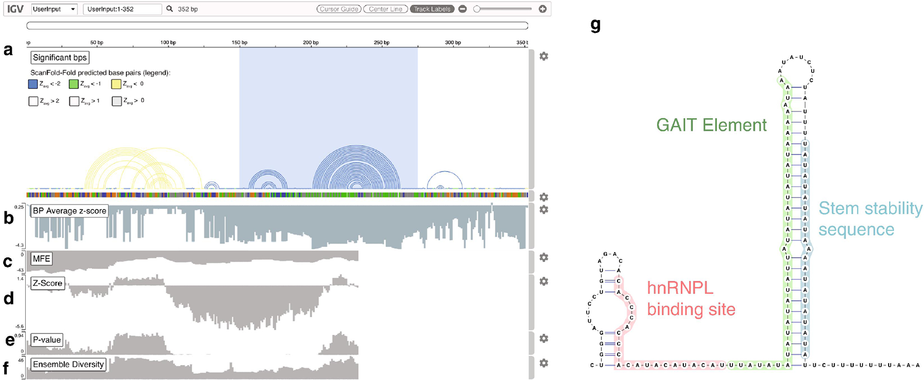
Example of RNA structural map created when using the ScanFold webserver’s example data. The example data is a portion of the human genome (HG38) extracted from the RNAStructuromeDB [37] which encompasses the VEGFA riboswitch (coordinates hg38|chr6:43,784,726..43,785,077). The sequence was run through the ScanFold webserver (https://mosslabtools.bb.iastate.edu/node/add/scanfold) using default settings (except step size, which was set to 1 nt). (a) The most significant base pairs are shown as arc diagrams. Here, arcs are colored based on their Z_avg score (yellow for < 0, green for < −1 and blue for < −2). The VEGFA translation permissive structure is highlighted with a blue box. Below the base pair arcs is the sequence track where nucleotides are colored based on their identity (guanine is orange, adenine is green, cytosine is blue and uracil is grey). (b) This track depicts the Z_avg score per nucleotide as a bar graph. Tracks (c) through (f) correspond to the results of ScanFold’s raw scanning window analysis, where the value of each labeled metric, corresponds to the first nucleotide of the window the metric was captured in. (g) This is the secondary structure corresponding to the blue highlighted region of the “Significant bps” track in track (a). The named portions of the riboswitch are labeled and colored accordingly.

2.2. Running ScanFold

The scanFold pipeline can be run using the scripts available on github (https://github.com/moss-lab/ScanFold) or can be accessed as a webserver tool (https://mosslabtools.bb.iastate.edu). This section focuses on running ScanFold as a webserver tool, however the main points apply to using the scripts as well. When using the webserver, the only requirement for running ScanFold is providing an input sequence. The ScanFold demonstrations that follow correspond to example data that can be run on the server. Here, we use a 352 nt sequence of RNA that encompasses the human VEGFA mRNA riboswitch (this example data can be loaded by clicking the “Load Example Data” button; Fig. S1a). Users can upload their own sequence by pasting a sequence directly into the text box (Fig. S1b) or by uploading a FASTA file (Fig. S1c); the webserver has a sequence size limit of 20,000 nt, while the scripts do not have any size restrictions. Below the sequence submission options are (optional) fields where users can give their submission a name (Fig. S1d; using the sequence’s accession number is recommended to simplify downstream analyses when using genome browsers such as IGV, see the example in section 5), provide an e-mail address (Fig. S1e) where a notification and link will be sent when results are complete, and a dropdown box that sets the length of time results will be available for viewing and/or download (Fig. S1f; one hour, one day [default], or one week). Following these, are parameters which alter the way ScanFold operates and impact results in meaningful ways, because of this, each of these fields will be described in detail along with suggestions and tips.

2.2.1. Window size

The first parameter to consider when running ScanFold (or any scanning window analysis) is the window size (Fig. S1g). This parameter is an integer value which dictates the length, in nucleotides (nt), of the fragment that will undergo folding analysis. Lange et. al. [31] found that a window size between 100 and 150 nt is optimal for maximizing accuracy and detecting known cis-regulatory structures in large mRNAs; where larger window sizes predict erroneous long-range pairs, and smaller window sizes underestimated the extent of known structure motifs. Our initial comparison of window sizes was in agreement with these findings where a window size of 120 nt performed best at accurately detecting and modeling known structures in both HIV-1 and ZIKV [25].

In Figure S2 different window sizes are shown to affect the ScanFold structural maps generated for the VEGFA riboswitch region. Here the Translation Permissive (TP) conformer of the VEGFA riboswitch is detected by window size 100 nt and only partially by window size 150 nt, while a window size of 200 or 40 nt fails to accurately detect the known model. This example illustrates that a window size between 100 and 150 nt is generally best for identifying and modeling functional structures, but in a case dependent manner.

Window sizes deviating from the optimal range between 100 and 150 nt do have potential applications. Smaller window sizes can be useful if specifically looking to identify motifs composed of smaller hairpins. The same is also true for larger hairpins. For example, in the HIV-1 genome, ScanFold was only able to detect the small terminal hairpins present in the large functional structured RNA, known as the Rev response element (RRE), but was unable to detect the basal stem, which spans > 350 nt (this was detected with a window size of 600 nt; see section 3.3 for details). Such large stems are detectable only if they are less than or equal in size to the chosen window size. Because of this, it may be beneficial to run multiple window sizes to check if any large stems have been ordered to form. The ScanFold webserver can make the process of testing multiple window sizes easy, as multiple jobs can be run quite rapidly (when attempting to optimize multiple parameters it may be beneficial to use larger step sizes to speed up the process; see section 2.2.2 below).

2.2.2. Step size

The step size field (Fig. S1h) is an integer value which dictates the number of nucleotides the scanning window steps downstream (sometimes referred to as slide). The step size is the parameter most directly governing the number of windows generated throughout the scan (depending on the sequence length and window size; Eq. 3). A 1 nt step size is recommended to maximize the number of windows which cover each nucleotide during the scan. For a sequence length (L) of 350 nt and window length (W) of 120 nt, a step size of 1 vs. 10 nt would result in difference of 230 vs. 23 windows respectively.

$$\mathit{\text{Number\hspace{0.17em}of\hspace{0.17em}Windows }}=\frac{L-W+1}{S}$$ #Eq. 3

The benefit to using a larger step size is to decrease computational time, which could be beneficial for multiple reasons. For example, scanning window analyses of large genomes (e.g. eukaryotic genomes) typically use large step sizes to obtain results in a reasonable amount of time (40 nt was used for RNAz [36] and ScanFold–Scan analyses of the human genome [37]). However, users may also want to perform rapid preliminary scans of multiple small sequences. As long as the step size is a fraction of the chosen window size, ensuring windows overlap, low z-score regions should be detected.

In Figure S3, the impact of using multiple step sizes is shown for our example data (all other parameters set to default). The TP conformer of the VEGFA riboswitch was detected by all four step sizes shown (1, 5, 10 and 40 nt). Indeed, the structural models predicted by each look quite similar. However, using a larger step size results in less window coverage. This reduces the ScanFold algorithm’s ability to discern which base pairs led to low z-scores.

2.2.3. Randomizations

The “randomizations” field (Fig. S1i) refers to the number of times the native sequence will be shuffled and folded during the calculation of each window’s ΔG° z-score. Higher randomizations will increase the robustness of results (by reducing variation between results; Table S1) but can increase computational time (in a linear fashion; doubling randomizations will roughly double computation time). For example, using the ScanFold webserver to scan the HIV-1 genome with a 120 nt window size, 1 nt step size, and 50 randomizations takes roughly 30 minutes and increasing randomizations to 500 increases computational time to roughly 5 hours.

2.2.4. Shuffle Type

The “Shuffle Type” field (Fig. S1j) refers to the type of shuffling to be used during calculation of the ΔG° z-score: mononucleotide (set by inputting “mono”) or dinucleotide (set by inputting “di”). During the calculation of the ΔG° z-score the randomized sequences serve as a negative control to determine if primary sequence has been ordered to fold more stably than expected. Generating an ideal negative control is a challenge: mononucleotide shuffling completely abolishes native order but disrupts background dinucleotide content (potentially overestimating z-score magnitude, as the energy model used in folding is a nearest-neighbor model); dinucleotide shuffling preserves this background, but requires a more complex shuffling routine (ScanFold uses Clote’s implementation of the Altschul and Erickson algorithm [38]). Our previous study compares the results of ScanFold using both mononucleotide and dinucleotide shuffling techniques: both perform well at detecting the known functional structures in HIV-1 and ZIKV and result in similar overall z-score trends across the genome (Fig. 6 of [25]) with dinucleotide shuffling z-scores being more positive overall and leading to slightly less base pairs being predicted with Z_avg < −2.

2.2.5. Temperature

The “Temperature” field (Fig. S1k) allows the user to change the temperature, in degrees Celsius, that is used during the calculation of ΔG° folding values during all MFE calculations. The default temperature is 37°C, however, this may be different based on the organism or experimental conditions being used.

2.2.6. Competition

As described previously [25], the ScanFold pipeline determines the best pairs per nucleotide in the input sequence (based on the Z_avg; Eq. 2). In some cases, during the initial analysis, a single nucleotide may be the best pairing partner for two or more separate partners; this is described as competition. The competition field (Fig. S1l) will determine whether or not ScanFold reports only the best partners among the competitors or reports all potential partners. If competition is turned off, all “best” pairs will be reported, but this will remove the “BP Average z-score” data (an example of which can be seen in Figure S4). This can be useful for visualizing the presence of competing structures with similar metrics.

2.3. ScanFold output

When a job completes on the ScanFold web server, results are depicted as comprehensive structural maps (described in Section 2.1 and shown in Figs. 1, S2–S4). All data depicted within are also available for download using links directly below the structural maps. The first link will allow users to download all results within a zipped folder. The contents of this folder are described in Table 1 (bolded entries are available as from individual download links as well).

Table 1.

Description of output files from ScanFold Webserver. There are 15 output files available in the “Download All Results” zip folder. Users can load 11 of these, marked “Y” in the IGV column, directly into the IGV desktop app (tested for versions 2.5.3 to 2.61). Bolded file extension denote files which are also available for individual download.

File extension	IGV	Description
.scan-out.tsv		Raw output of ScanFold-Scan. Traditional scanning window output, showing all metrics calculated per window including MFE, z-score, p-value, dot-bracket structure, and centroid structure.
.mfe.wig	Y
.ed.wig	Y	These are “wig” format files corresponding to values from the ScanFold-Scan ouput.
.zscore.wig	Y
.pvalue.wig	Y
.bp	Y	IGV base pair track. The “.bp” format describes the connections between nucleotides and the header contains information such as the color used to depict the arc. For proper loading in IGV, IGV must first be loaded with the “input.fa” and “.fai” files below.
.final_partners_zscore.wig	Y	This is another “wig” format file which reports the Zavg values corresponding to the arrangements depicted in the “.bp” track above.
.input.fa	Y	This is the FASTA file containing the sequence which was scanned. The header is set as the “Input Name” set be the user (Default: UserInput).
.fai	Y	This is the index file for the FASTA file above, and is used by IGV.
.−1filter.ct	Y	Structure model files showing base pair arrangments whose Zavg scores are less than the filter value stated in extension. The “CT” files are connectivity files and can be opened in programs such as VARNA, IGV, and RNAstructure.
.−2filter.ct	Y
.nofilter.ct	Y
.−2filter.dbn	Y
.final_partners.txt		This is output from ScanFold-Fold and list the “best” arrangments for each nucleotide sequence as well as the corresponding average metrics observed.
.log.txt		Raw output of ScanFold-Fold. This will give the list of all base pairs predicted for each nucleotide, the number of windows each are observed in, and the average metrics for each.

The output from the ScanFold–Scan step (extension “.scan-out.tsv”) is a tab separated file, where each row corresponds to a window and its corresponding metrics (the MFE, z-score, p-value and ED metrics correspond to the “.wig” tracks available for download and depicted in Fig. 1d–g). The output from ScanFold–Fold consists of the lowest Z_avg base pair arrangements and their corresponding Z_avg values (Fig. 1a and 1b) as well as log files detailing the pairing partners of each nucleotide in the input sequence.

3. Characterizing ScanFold results

ScanFold attempts to map the structural landscape of RNAs to highlight regions of interest, but was not developed to explicitly predict the global structure of large RNAs. Unlike thermodynamic folding algorithms (which choose base pairing patterns based on their contribution to the most globally stable structure), ScanFold chooses the best local arrangement for all nucleotides based on their ability to generate the lowest thermodynamic z-scores. Therefore, in regions where primary sequence contains a specific negative z-score generating structure, discrete structures are easily modeled (e.g. nt 150–275 in Fig 1.). In our original report, base pairs with Z_avg scores < −2 overwhelmingly corresponded to the known functional RNA structures in the HIV-1 and ZIKV genomes; interpreting strong z-score signals in these regions was therefore relatively straight-forward. In regions with unremarkable z-scores (e.g. 0 > Z_avg > −1), interpreting results is less clear; the modeling process may select base pairs from overlapping structures (e.g. nt 1–100 in Fig. 1). Possible interpretations for these regions (which, by their nature, are more common) were not previously explored. Therefore, in an attempt to aid interpretations for the entirety of ScanFold results, this section is dedicated to characterizing the relationship between ScanFold results and two of the most widely utilized RNA structural analysis methods utilized today: SHAPE probing and thermodynamically calculated pairing probabilities.

3.1. Arrangements of low Z_avg nucleotides agree with pairing probabilities

Previous studies report a correlation between the z-score of a sequence and its Shannon entropy (a measure of the sum of all pairing probabilities) [39]. To determine if this correlation persists at a per-nucleotide level we carried out a comparison between the Z_avg values predicted for each nucleotide of the HIV-1 and ZIKV genomes (using the results from [25]) to pairing probabilities predicted by RNAplfold, a program specializing in rapidly computing pairing probabilities for large RNA sequences [27]. Overall the correlation between Z_avg and probabilities for HIV-1 was modest (correlation coefficient of −0.21). However, unlike pairing probabilities, Z_avg scores do not suggest whether a nucleotide is paired or unpaired. Therefore, a separate analysis was carried out, which the binary paired/unpaired states of ScanFold predictions to RNAplfold results that were transformed to define nucleotides as paired or unpaired based on their probability (see section 4.1)—thus allowing for direct comparisons between the two metrics. The paired/unpaired states of nucleotides predicted by each program were then compared to determine how often they match (results shown in Table 2). Here, it was found that RNAplfold and ScanFold’s paired/unpaired predictions were in agreement for 68.7% of nucleotides in HIV-1 and 80.2% of nucleotides in ZIKV. On average, the matches appear to have an inverse relationship to Z_avg scores (where lower Z_avg scores correspond to higher matches; Fig. S5).

Table 2.

Results of SHAPE and BP probability comparisons using different Z_avg filters. The percentage of paired and unpaired states which match between RNAplfold (PL), ScanFold (SF), and the HIV-1 genome reference structure reported in Watts et. al 2009 (W09) are listed per Z_avg region. Following these matches are the average (μ) and median (M) base pairing probabilities (BP) and SHAPE reactivity (SR) values for nucleotides within each filtered region.

	HIV-1					ZIKV
Zavg	SF = PL(%)	SF = W09(%)	PL = W09(%)	BP(μ(M))	SR(μ(M))	SF = PL(%)	BP(μ(M))	SR(μ(M))
All	68.680	62.804	72.648	0.445(0.438)	0.407(0.330)	80.263	0.559(0.604)	0.467(0.269)
>=0	43.090	41.400	79.360	0.343(0.288)	0.451(0.430)	43.438	0.407(0.378)	0.656(0.549)
<0	74.321	66.565	71.168	0.468(0.473)	0.397(0.310)	82.581	0.569(0.622)	0.455(0.258)
<−1	77.205	74.903	73.054	0.502(0.522)	0.367(0.250)	85.523	0.607(0.685)	0.407(0.182)
<−2	81.400	85.700	79.700	0.560(0.620)	0.319(0.130)	89.069	0.653(0.769)	0.363(0.055)

When filters are applied to only consider regions where Z_avg nucleotides are less than −1 and −2 (by default ScanFold filters results based on these cutoffs), the percentage of ScanFold results that match RNAplfold increase to 77.2 and 81.4% respectively (Table 2). When looking at these filtered regions further, a clear trend could be observed, where lower Z_avg filters corresponded to higher average base pair probabilities (Table 2 and Fig. 2a). The same trends were observed for the ZIKV genome (Fig. 2b), with match percentages of 80.3, 85.5 and 89.1 for the full genome, Z_avg < −1, and Z_avg < −2 respectively (Table 2). Conversely, in regions where Z_avg scores were greater than or equal to 0, matches were low (43.1% in HIV and 43.4% in ZIKV; Table 2. and Fig. 2).

Figure 2.

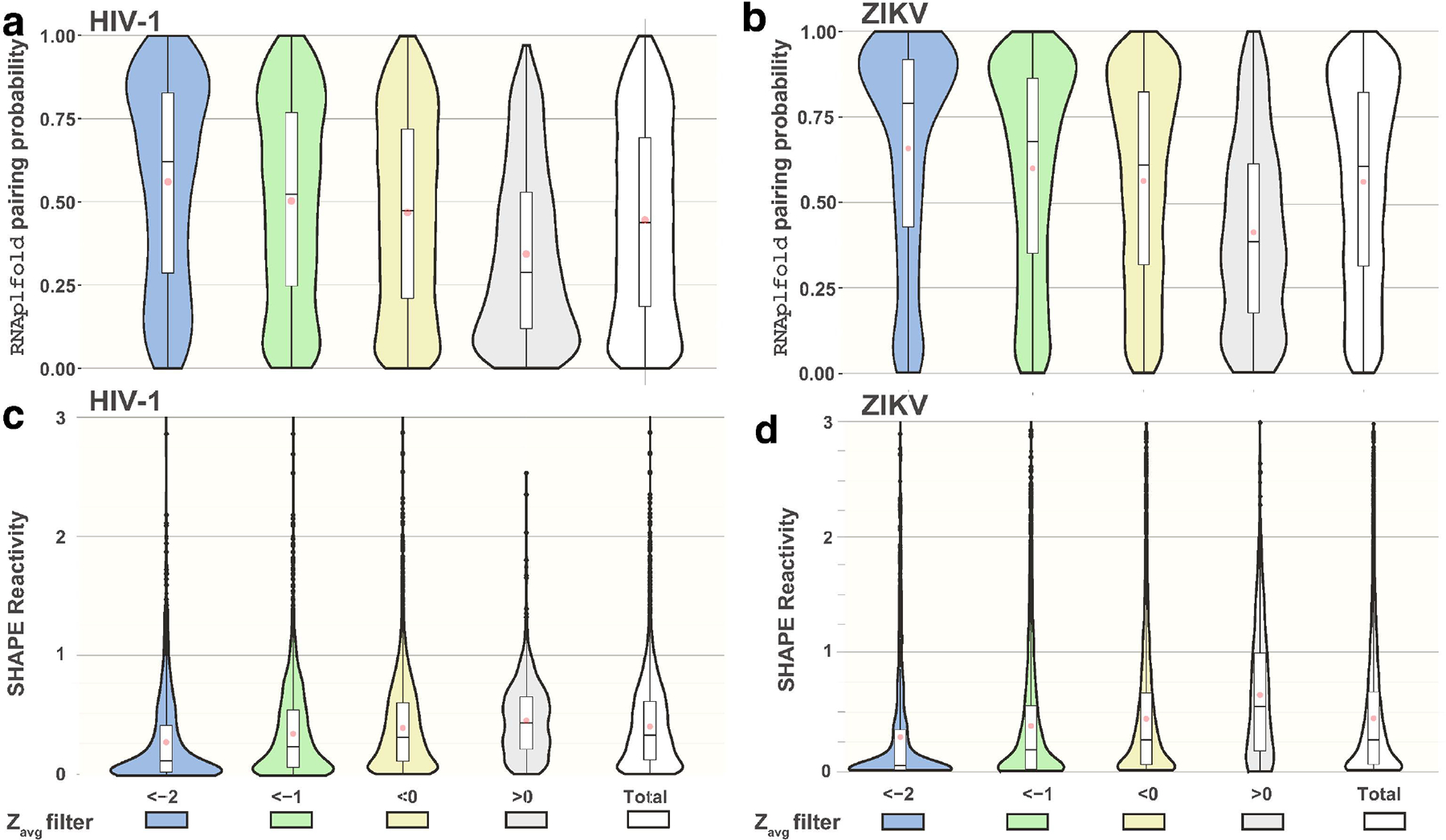
Violin and Box and Whisker plots depicting the distribution of SHAPE reactivities and base pairing probabilities based on the nucleotides Z_avg scores. For each genome only nucleotides passing a Z_avg filter threshold were counted in the creation of violin plots and box and whisker plots. (a-b) The distribution of base pairing probabilities based on Z_avg scores for the HIV-1 (a) and ZIKV (b) genomes. (c-d) The distribution of SHAPE reactivities based on Z_avg scores for the HIV-1 (c) and ZIKV (d) genomes. Violin plot width is proportional to the number of nucleotides with the corresponding SHAPE or base pairing probability. Box and whisker plots depict the spread of values as follows: center lines show the medians red dots show the mean; box limits indicate the 25th and 75th percentiles; whiskers extend 1.5 times the interquartile range from the 25th and 75th percentiles, outliers are represented by dots. Graphs were generated using ggplots library in R. Full data can be seen in Supplementary Dataset 2.

Paired/unpaired states were also compared to a reference structure for the HIV-1 genome [40] to determine how well RNAplfold and ScanFold matched data-driven structure models (i.e. informed by SHAPE reactivity). RNAplfold performed best overall and was able to accurately predict the state of 72.7% of nucleotides, while ScanFold predicted 62.8% (Table 2). The lower overall accuracy of ScanFold can be mostly attributed to the low accuracy for nucleotides with positive Z_avg scores (where ScanFold accuracy was 41.4% on average). Conversely, the best local performance for both programs, can be seen for nucleotides with Z_avg scores less than −2; this accounts for 1000 nt in HIV-1 (roughly 1/9^th of the genome). Here, ScanFold performed the best, accurately predicting 85.7% of nucleotide states whereas, RNAplfold predicted 79.7% (Table 2).

3.2. Low Z_avg nucleotides correspond to lower SHAPE reactivity

The observation that low Z_avg nucleotides (Z_avg < −2) corresponded to higher pairing probabilities and were best at predicting the paired states of nucleotides from SHAPE directed models, suggested a potential relationship between SHAPE reactivity and low z-score regions. The SHAPE reactivity of a nucleotide is most directly related to its secondary structure; higher reactivity values relate to lower pairing probabilities and, conversely, lower reactivities correspond to higher pairing probabilities. Therefore, low Z_avg regions may be characterized by a higher number of low SHAPE reactivity nucleotides, just as they are comprised of a greater number of high pairing probability nucleotides Fig. 2a–b.

The average and median normalized SHAPE reactivities reported for the HIV-1 genome are 0.41 and 0.33 respectively. When SHAPE reactivity values are filtered based on their corresponding nucleotide’s Z_avg score, a similar trend to pairing probabilities appears (Table 2 and Fig. 2c). For the nucleotides with Z_avg < −2, the mean and median SHAPE reactivity values drop down to 0.32 and 0.13 respectively. Interestingly, for nucleotides with positive Z_avg scores, mean and median SHAPE reactivity values increase to 0.45 and 0.43. Again, these trends follow for the SHAPE reactivity values reported for ZIKV genome [41]. The average and median SHAPE reactivities reported for the ZIKV genome are 0.46 and 0.27 respectively (Table 2 and Fig. 2d) and for nucleotides with Z_avg < −2, the mean and median SHAPE reactivity values drop down to 0.36 and 0.05 respectively. Again, for nucleotides with positive Z_avg scores, mean and median SHAPE reactivity values increase to 0.65 and 0.54 respectively.

3.3. Low Z_avg nucleotides correspond to more accurate secondary structure predictions

The observations in sections 3.1 and 3.2 indicate that low Z_avg ScanFold results are comparable to experimental probing and accessibility calculations in the analysis of HIV-1 and ZIKV RNA structural propensity. These comparisons, however, did not consider the accuracy of secondary structures modeled by these low Z_avg nucleotides. To assess the accuracy of ScanFold models, two scoring metrics, sensitivity (Eq. 4) and positive predictive value (PPV; Eq. 5), were calculated using the scorer program from the RNAstructure package (see section 4.3 for details). Calculated scores are compared to those using RNAfold models (as this is the underlying folding algorithm used by ScanFold) to demonstrate how ScanFold differs from single sequence folding algorithms.

$$\mathit{\text{PPV}}=\frac{\mathit{\text{True\hspace{0.17em}}}\mathit{\text{Predicted\hspace{0.17em}}}\mathit{\text{Base\hspace{0.17em}Pairs}}}{\mathit{\text{Total\hspace{0.17em}}}\mathit{\text{Predicted\hspace{0.17em}}}\mathit{\text{Base\hspace{0.17em}Pairs}}}$$ #Eq. 4

$$\mathit{\text{Sensitivity}}=\frac{\mathit{\text{True\hspace{0.17em}}}\mathit{\text{Predicted\hspace{0.17em}}}\mathit{\text{Base\hspace{0.17em}Pairs}}}{\mathit{\text{Total\hspace{0.17em}}}\mathit{\text{Reference\hspace{0.17em}}}\mathit{\text{Base\hspace{0.17em}Pairs}}}$$ #Eq. 5

The results of scoring can be seen in Figure 3 and Table 2. RNAfold, using a maximum base pair span of 600 nt (the same constraint used during the generation of the reference structure [40]) resulted in the best sensitivity of all tested approaches (Fig. 3a). The next best sensitivity was found using ScanFold with a window size of 600 nt, likely due to the accurate prediction of the 354 nt long hairpin (spanning nt 7245–7599 nt), which is not detectable by other window sizes. The other two models generated by RNAfold had the next best sensitivities (0.416 for unconstrained fold and 0.392 for max base pair span of 120 nt). For the remainder of ScanFold results, sensitivity is less than 0.30 on average; this is expected, as ScanFold consensus structures predict fewer base pairs with stricter average z-score filters.

Figure 3.

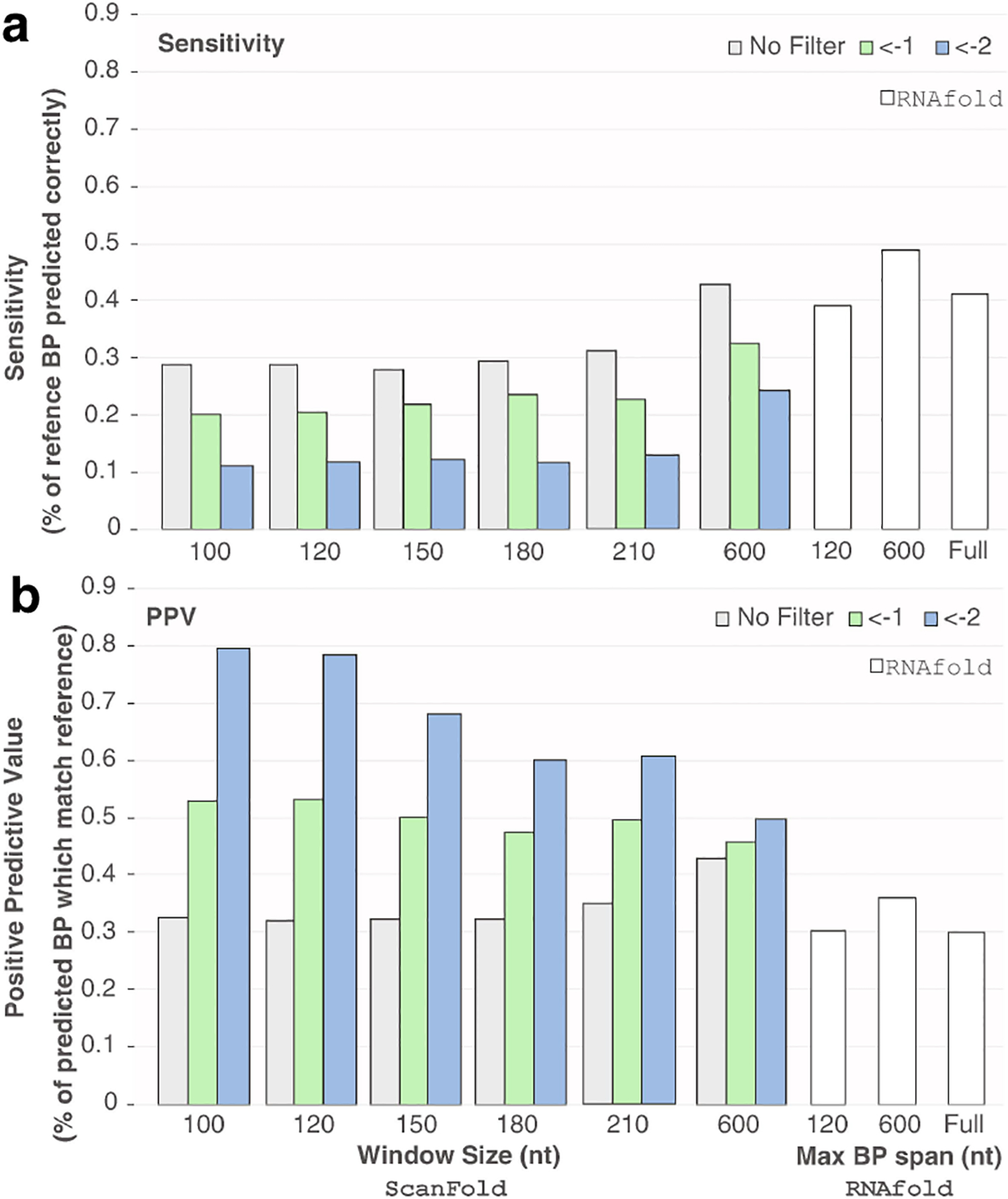
The positive predictive values and sensitivities for RNAfold and ScanFold predicted structures of the HIV-1 genome. The reference structure for all HIV-1 scores was generated from the secondary structure reported in [40]. All scoring was done using RNAstructure’s scorer program. Positive predictive value (PPV) measures the % of predicted base pairs which were correct (Eq. 4) and the sensitivity measures the number of base pairs in the reference structure which were correctly predicted (Eq. 5). (a-b) The sensitivity (a) and PPV (b) of ScanFold generated CT files from [25] and RNAfold generated structures. The CT files for ScanFold structures with window sizes 100 to 210 were all taken directly from the supplementary data of [25], and the 600 nt window size results were generated using the ScanFold webserver (all window sizes are labeled under the ScanFold results on the left side of each graph). Each ScanFold CT file corresponds to structures with nucleotides having Z_avg scores less than the listed filter value: no filter (grey), < −1 (green) and < −2 (blue). RNAfold predictions of HIV-1 were conducted to generate dot bracket files for the global fold (labeled “Full”) as well as the max base pair span restricted models (restricted to 120 and 600 nt; lableled approriately). Scores for these three structures are shown on the right side of both (a) and (b) and colored white.

The best PPVs are seen for all ScanFold results, with Z_avg <−2 structures (Table Fig. 3b and Table 2). This is consistent with the results from sections 3.1 and 3.2, which show that the paired/unpaired nature of nucleotides with Z_avg < −2 are better predicted than others; the corresponding secondary structures tested here have the highest PPVs. Among these, however, the best PPVs can be seen for window sizes 100 and 120 nt, which had PPVs of 0.795 and 0.784, respectively (window size 120 nt had the higher sensitivity—accurately predicting 18 more base pairs of the reference structure). Thus, the ScanFold predicted structures contain fewer, but more accurately predicted, base pairs (yielding lower sensitivity and higher PPV).

3.4. Interpreting Z_avg scores

When using ScanFold with optimal parameters (i.e. step size of 1 nt and window sizes between 100 and 150 nt), regions with Z_avg scores < −2 correspond to nucleotides with lower SHAPE reactivity (Fig. 2a–b) and higher base pairing probabilities (Fig. 2c–d) across the HIV-1 and ZIKV genomes. This suggests that regions with Z_avg scores < −2 are more likely to be structured (based on both experimental and thermodynamic data). Importantly, the ScanFold generated secondary structures that correspond to these nucleotides are have ~80% PPV for both the HIV-1 genome reference structure (Fig. 3) and the reference structures in the untranslated regions of ZIKV (Supplemental Table 8 of [25]).

Z_avg regions between −1 and 0 appear to contain primary sequences that form thermodynamically stable structures, but do not correspond to SHAPE reactivities or base pairing probabilities much different from the data in aggregate (Fig. 2; compare < 0 results to Total values). Further, the secondary structure models generated by ScanFold for these regions (< 0) do not appear any more accurate than RNAfold (Fig. 3; compare “No Filter” results to those of RNAfold).

Positive Z_avg regions highlight primary sequences that do not form structures amenable to modelling (either experimental or thermodynamic); potentially due to dynamics, non-canonical base pairing, or complex tertiary structures. Thus, the presence of functional RNA structures in these regions should not be ruled out as a possibility. Another intriguing possibility, that needs additional study, is that some of these regions (especially if they have Z_avg scores > 2) may actually have been ordered to avoid forming structure, such as the case near ribosomal binding sites [42], musashi binding sites [43], or facilitating the formation of functional intermolecular interactions [44].

4. Methods

The HIV-1 genome sequence used for all analyses was taken directly from [40] and can be found in Supplementary Dataset 1 as well. The ZIKV genome was taken from the RefSeq genome with accession ID KJ776791.2.

4.1. Pairing probability analysis

RNAplfold (version 2.3.3) was used to calculate the unpaired probabilities for each nucleotide of the HIV-1 genome sequence (using command “rnaplfold −w 120 −u 1”). Using the resulting probabilities, each nucleotide was set to being paired whenever probability was above 50% (with this cutoff performing best at matching the paired unpaired states of the Watts et. al 2009 structure). In order to determine the ScanFold predicted pairing state for each nucleotide the “Final Partners” output file was used; this file reports the best pairing partner for each nucleotide along with the corresponding average MFE, z-score (Z_avg), and ensemble diversity values (Supplementary Dataset 1; extension “final_partners.txt”). Importantly, the Z_avg scores for each nucleotide are reported before competition has been filtered (competition is noted in the file, however), therefore, these values may correspond to a nucleotide which has actually been left unpaired in the final structural model. The results for competition-filtered data can be seen in Supplementary Dataset 2.

4.2. SHAPE reactivity analysis

SHAPE reactivity values for HIV-1 were taken from Data Set 2 of [40] and for ZIKV, SHAPE reactivities were taken from Supplementary Data 1 of [41] (labeled there as ZILM_SHAPE); all negative reactivity values were set to 0. When computing mean and median values, the first 11 and the final 31 nt of HIV-1 were ignored and for ZIKV, all values equal to −999 (missing data) were ignored.

4.3. Secondary structure prediction scoring

The reference structure for all HIV-1 scores was generated from the secondary structure reported in [40]. The reference structure’s helix file (reported in Supplementary Data File 1 [40]) was first converted to a dot bracket structure using the R package R4RNA and finally converted to a CT file (the format used in the scorer program) using the dot2ct function from the RNAstructure package. The CT files for ScanFold structures with window sizes 100 to 210 were all taken directly from the supplementary data of [25], and the 600 nt window size results (using a step size of 1 nt, and 100 mononucleotide randomizations) were generated using the ScanFold webserver. RNAfold (version 2.3.3) predictions of were conducted using the command line version to generate dot bracket files for the global fold as well as the max base pair span restricted constructs (using command “−maxBPspan=” 120 or 600 nt). The RNAstructure program dot2ct was used to convert the resulting RNAfold structures into CT files. All scoring was done using RNAstructure’s scorer program (Version 6.0; using exact enforcement with command “scorer −e”). The scorer program calculates the positive predictive value (PPV) and sensitivity metrics to quantify the accuracy of predicted structures versus a reference structure; PPV measures the % of predicted base pairs which were correct (Eq. 4) and the sensitivity measures the number of base pairs in the reference structure which were correctly predicted (Eq. 5).

5. Example using the HIV-1 genome

5.1. Browsing ScanFold results

Using the ScanFold webserver, the HIV-1 genome sequence was scanned using default settings (except step size and randomizations, which were changed to 1 nt and 50 respectively). The process was completed within 34 minutes and results were nearly identical to those reported originally. The information in ScanFold’s structural maps are well suited for genome browsers. Because of this, the ScanFold web server output is formatted to allow for viewing immediately on the IGV.js viewer loaded on the ScanFold results pages or for loading directly into the IGV desktop app (available here https://software.broadinstitute.org/software/igv/download). To do this, we first retrieve all necessary files by simply using the “Download All Results” link on the ScanFold results page (available in Supplementary Dataset 1 as well). Next, from within an open IGV desktop app, the FASTA file is loaded from the results folder as a “genome” (via the “File > Load Genome File…” option); this FASTA file has the extension “.input.fa”. This allows one to then load all IGV compatible files (Table 1) directly into IGV (either by dragging files directly onto IGV or opening via the “File > Load From File…” option). From here, all IGV features are available to view and analyze results. For this example, IGV was also loaded with (1) the results of a RegRNA [29, 45] scan set to specifically identify known cis-regulatory elements from Rfam [46–53] and (2) SHAPE reactivity data from Watts et. al. 2009, which was converted to a compatible WIG format for displaying values as heatmaps. The RegRNA data track was generated from the tab delimited output of RegRNA using the script “REGRNA_to_BED_GFF3.py” which is available in Supplementary Dataset 1.

In Figure 4, an example IGV setup depicting the first ~400 nt of the HIV-1 genome is shown (all of the files from this example are available in Supplementary Dataset 1 if readers wish to browse the entirety of results). Using this setup allows for rapid interpretations of ScanFold results. Attention is immediately drawn to the motifs depicted by blue arcs in the ScanFold “Significant BPs” track (from nt 1–100). The Z_avg scores corresponding to the nucleotides of the first stem are highly negative (< −3) and the following motif is slightly less negative with the basal stem nucleotides yielding Z_avg scores between −1 and −2. Inspecting the SHAPE reactivity track allows for an immediate visual check on the predicted base pairs; indeed highly reactive base pairs in this region (in red) correspond to unpaired nucleotides in their bulges and loops while less reactive nucleotides correspond to nucleotides predicted by ScanFold to be paired. The RegRNA track confirms that these structures correspond to the TAR hairpin and the “poly-a stem” from HIV-1 [40].

Figure 4.

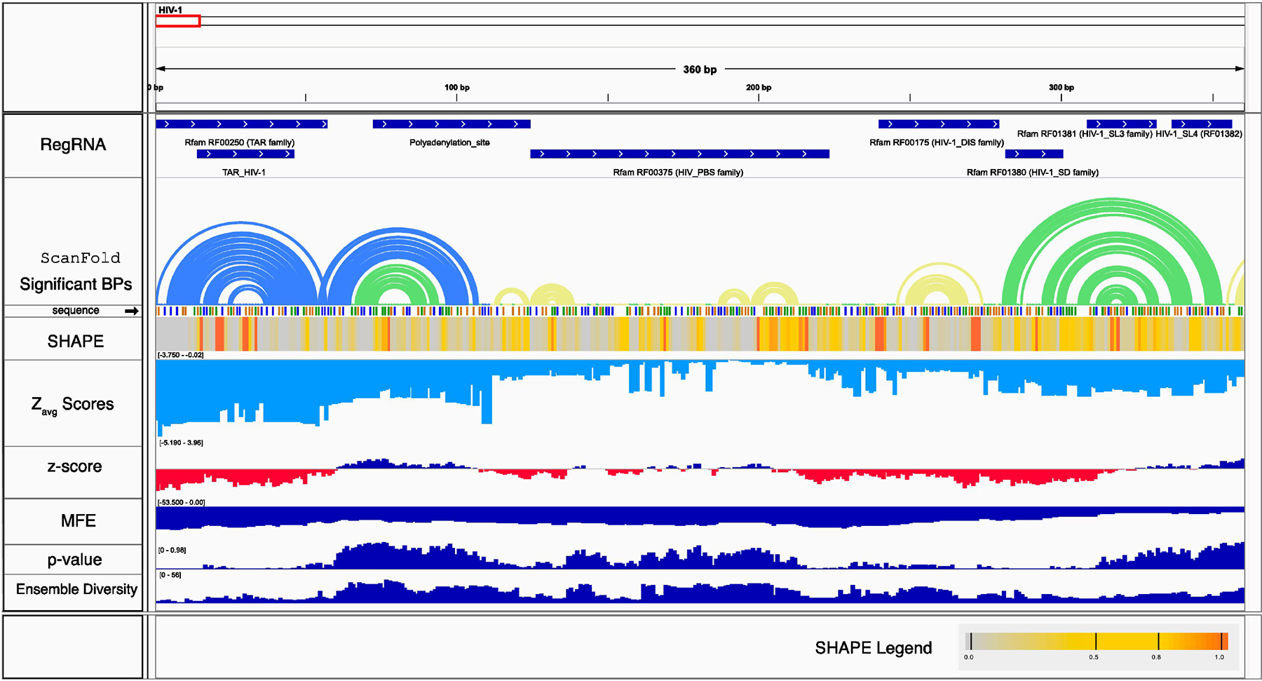
Example of IGV setup used to browse ScanFold results. Here the first ~400 nt of the HIV-1 genome is shown along with 9 tracks to aid in structural interpretations. The first track (in top to bottom order) is the RegRNA track which was generated by scanning the HIV-1 genome using the RegRNA webserver. The next track depicts the most significant base pairs predicted by ScanFold as arc diagrams. Here, arcs are colored based on their Z_avg score (yellow for < 0, green for < −1 and blue for < −2). The sequence track depicts the nucleotide identity using color where guanine is orange, adenine is green, cytosine is blue and uracil is grey. The SHAPE track shows a heatmap based on the reactivity value (legend in bottom left hand corner). The light blue Z_avg track shows the Z_avg scores of each nucleotide in the sequence. The following tracks are as described in Figure 1 (d–g). The range for all values is shown on the left hand side of each track in brackets as [low-high]. All tracks and their corresponding files can be found in Supplementary Dataset 1.

Downstream of this, the RegRNA track annotates the HIV primer binding site (PBS) region which corresponds to nucleotides with middling Z_avg scores (mostly between −1 and 0) and where the base pair track lacks unusually stable structural motifs. This region, consistent with the results in section 3.3, does not perform well at predicting the global reference structure for HIV-1; this could be due to fact that 18 nucleotides of the PBS region (ñt 200) are evolved to bind to intermolecular nucleotides from the Lys3 tRNA (a process which ultimately initiates reverse transcription [54]) where the presence unusually stable structures may be detrimental. However, it should be noted that the small hairpin predicted at ~190 nt, was later found to have 3 of its 4 base pairs structurally conserved between three HIV related RNA genomes [55].

The following four Rfam annotations in the RegRNA track correspond to the retroviral psi packaging element, which consists of four stem loop structures. Only one these, however, is detected and modeled correctly by ScanFold: the dimerization initiation site (DIS), which can be seen near nt 250. The following three stem loops, which are each < 20 nt in length, are not detected. Instead, ScanFold predicts a somewhat more stable than expected structure (with Z_avg nucleotides < −1) consisting of several bulges and a single tetraloop that are consistent with SHAPE reactivity; interestingly, this suggests this alternative structure may indeed form at some point during probing analysis.

5.2. Aiding downstream analyses

One benefit to the ScanFold method, over traditional scanning window analyses, is that a single structural model is generated for consideration. This is ideal for downstream analyses. The CT files generated by ScanFold (Table 1) can each be tested directly against aligned sequences to determine the frequency and type of base pairs which occur at each site throughout the alignment, as was done for proposed structural motifs in Influenza A [18]. The resulting base pair counts can suggest whether a structure is conserved (e.g. if most base pairs observed throughout the alignment are consistent with predicted structure) and provide further support that a predicted motif serves a functional role.

The highly negative Z_avg base pairs detected by ScanFold also serve as ideal targets for experimental structure-function analyses. Their correlation to lower SHAPE reactivity and higher base pairing probabilities in ZIKV and HIV-1 suggest that their formation in other RNA sequences, whether functional or not, is more likely than in regions with positive Z_avg scores. In this way, ScanFold can point researchers to areas that are well suited for functional analyses, because they are more likely to be amenable to modeling. When planning mutational analyses, tools such as RNA2dMut [56], can be used to design mutations specifically targeted to disrupt the most significant ScanFold predicted structures. Designing mutants based on the most significant structures generated by ScanFold can allow researchers to rapidly design targeted analyses; as was done recently for the most significant results in the mRNA of the human MYC oncogene [57].

6. Conclusions

ScanFold results can aid experimental design by rapidly characterizing large RNA molecules. ScanFold identifies, with confidence, local motifs that are likely to be functional and models of their secondary structures. In this way, ScanFold can help highlight motifs that can serve as ideal candidates for functional analyses and present structural models to aid in experimental design or that provide the basis for additional structural characterizations at higher resolution (e.g. using NMR, crystallography, etc.).

Supplementary Material

1

Figure S1. Screen shot of the ScanFold webserver submission page. The ScanFold webserver was accessed on July 25^th 2019 from the ScanFold (Full Pipeline) link at https://mosslabtools.bb.iastate.edu/scanfold.

2

Figure S2. Relationship between regions where ScanFold and RNAplfold predictions of paired or unpaired states match and computed Z_avg scores. The average (over 120 nt) number of matches between ScanFold and RNAplfold predictions of the paired/unpaired state of each nucleotide in the (a) HIV-1 genome and (b) ZIKV genome. Green lines depict the moving average number of matches corresponding to the percentage values shown on the left axis. Blue lines depict the value of Z_avg scores for each nucleotide of the sequence. Regions where Z_avg scores dip below −2 (red line) are highlighted in gold.

3

Figure S3. Example of the effect window size has on ScanFold results of the VEGFA example data. Window sizes between 100 and 150 are consider optimal. A window size of 100 detects the main hairpin of the Translation Permissive (TP) conformer of the VEGFA riboswitch, while the other window sizes fail to detect, or only partially detect it. Interestingly, the small window size (40 nt) is able to successfully predict the Translation Silencing (TS) conformer of the VEGFA riboswitch (which is composed of two smaller hairpins, less than 40 nt in length, composed of nucleotides from within the large hairpin of the translation permissive form). Structural maps are the same as described in Figure 1.

4

Figure S4. Example of the effect window size has on ScanFold results of the VEGFA example data. Structural maps are the same as described in Figure 1.

5

Figure S5. Example of ScanFold results when “competition” filter is turned off. Here overlapping and competing base pairs are allowed to be depicted, however, this restricts the ability to show corresponding Z_avg scores, which leaves the “BP Average z-score” track empty. The four final tracks are as described in Figure. 1.

6

Supplementary Dataset 2. This excel spreadsheet file holds the raw data used to compare SHAPE reactivities, base pairing probabilities, and the Watts 2009 HIV-1 reference structure to ScanFold results for ZIKV and HIV-1 genomes as reported in [25]. Methods describing the acquisition of data can be found in Section 4.

7

Supplementary Dataset 1. This zipped folder contains the results of a ScanFold scan of the HIV-1 genome retrieved from Watts et. al 2009[40]. The scan was performed using the ScanFold webserver with a 1 nt step size, 120 nt window, and 50 randomizations (all other settings at default). These results are within a subfolder titled “DownloadAllResults”; the contents of which are described in Table 1. Outside this folder, the file named “DS2seq.shape.wig” can be loaded into IGV (see Section 5) to browse the results of the ScanFold scan. The file name “RegRNA_HIV-1.gff3” can also be loaded into IGV and contains the results of a RegRNA [29, 45] scan to search for Rfam hits in the HIV-1 genome sequence. The script provided here titled “REGRNA_to_BED_GFF3.py” can be used to generate GFF3 files for genome browsers using the tab delimited output of RegRNA.

Table 3.

Sensitivity and positive predictive values for secondary structure models predicted for the HIV-1 genome. Here the reference structure is the secondary structure reported for HIV-1 genome reported by Watts et. al. (2009). Method names for ScanFold refer to the window size used in parentheses, and for RNAfold, the max bp span used is in parentheses. For scoring, the HIV-1 genome reference structure was generated using the secondary structure reported in Watts et. al 2009. Predicted structures from RNAfold were generated using three different settings: (1) the MFE fold predicted for the entire genome [RNAfold] (2) the MFE fold for a max bp span of 120 nt [RNAfold(120nt)]and (3) an MFE fold using a max bp span of 600 nt [RNAfold(600nt)] (the setting used for the original modelling). The scanFold predicted structures (for windows sizes 100 to 210 nt) were taken directly from the supplemental CT files of Andrews et. al. 2018, here step sizes were 1 nt, randomizations were 50, and shuffling was mononucleotide; an additional prediction was performed using a window size of 600 nt directly on the webserver (step size of 1 nt and 50 randomizations). The sensitivity and positive predictive value (PPV) for each of the predicted secondary structures was calculated using the RNAstructure package’s scorer program (using exact enforcement).

	PPV (HIV-1)			Sensitivity (HIV-1)
Method	Total	Zavg < −1	Zavg < −2	Total	Zavg < −1	Zavg < −2
ScanFold(100nt)	0.325	0.529	0.795	0.284	0.2	0.111
ScanFold(120nt)	0.319	0.531	0.784	0.287	0.206	0.121
ScanFold(150nt)	0.323	0.500	0.682	0.279	0.218	0.12
ScanFold(180nt)	0.322	0.474	0.602	0.292	0.23	0.114
ScanFold(210nt)	0.349	0.495	0.607	0.315	0.246	0.124
ScanFold(600nt)	0.428	0.456	0.498	0.426	0.317	0.236
RNAfold(120nt)	0.304			0.392
RNAfold(600nt)	0.361			0.493
RNAfold	0.301			0.416

Highlights.

Demonstration of ScanFold, a single sequence method for RNA structural motif discovery.

ScanFold is available via a user-friendly webserver or for download.

Example usages and data are provided using the HIV-1 and ZIKV genomes.

Comparisons are made to available experimental data sets from ZIKV, HIV-1, Hepatitis C and Dengue Virus, to indicate the robustness of the approach.

Comparisons are made to other single sequence approaches to show how ScanFold can complement available methods.

References

- [1].Weik M, Modrof J, Klenk HD, Becker S, Muhlberger E, Ebola virus VP30-mediated transcription is regulated by RNA secondary structure formation, J Virol, 76 (2002) 8532–8539. [DOI] [PMC free article] [PubMed] [Google Scholar]
- [2].Dingwall C, Ernberg I, Gait MJ, Green SM, Heaphy S, Karn J, Lowe AD, Singh M, Skinner MA, HIV-1 tat protein stimulates transcription by binding to a U-rich bulge in the stem of the TAR RNA structure, EMBO J, 9 (1990) 4145–4153. [DOI] [PMC free article] [PubMed] [Google Scholar]
- [3].Levengood JD, Rollins C, Mishler CH, Johnson CA, Miner G, Rajan P, Znosko BM, Tolbert BS, Solution structure of the HIV-1 exon splicing silencer 3, J Mol Biol, 415 (2012) 680–698. [DOI] [PubMed] [Google Scholar]
- [4].Moss WN, Dela-Moss LI, Priore SF, Turner DH, The influenza A segment 7 mRNA 3’ splice site pseudoknot/hairpin family, RNA Biol, 9 (2012) 1305–1310. [DOI] [PMC free article] [PubMed] [Google Scholar]
- [5].Tolbert M, Morgan CE, Pollum M, Crespo-Hernandez CE, Li ML, Brewer G, Tolbert BS, HnRNP A1 Alters the Structure of a Conserved Enterovirus IRES Domain to Stimulate Viral Translation, J Mol Biol, 429 (2017) 2841–2858. [DOI] [PMC free article] [PubMed] [Google Scholar]
- [6].Wilson W, Braddock M, Adams SE, Rathjen PD, Kingsman SM, Kingsman AJ, HIV expression strategies: ribosomal frameshifting is directed by a short sequence in both mammalian and yeast systems, Cell, 55 (1988) 1159–1169. [DOI] [PubMed] [Google Scholar]
- [7].Dreher TW, Miller WA, Translational control in positive strand RNA plant viruses, Virology, 344 (2006) 185–197. [DOI] [PMC free article] [PubMed] [Google Scholar]
- [8].Das AT, Klaver B, Berkhout B, The 5’ and 3’ TAR elements of human immunodeficiency virus exert effects at several points in the virus life cycle, J Virol, 72 (1998) 9217–9223. [DOI] [PMC free article] [PubMed] [Google Scholar]
- [9].Shen R, Miller WA, Structures required for poly(A) tail-independent translation overlap with, but are distinct from, cap-independent translation and RNA replication signals at the 3’ end of Tobacco necrosis virus RNA, Virology, 358 (2007) 448–458. [DOI] [PMC free article] [PubMed] [Google Scholar]
- [10].Akiyama BM, Laurence HM, Massey AR, Costantino DA, Xie XP, Yang YJ, Shi PY, Nix JC, Beckham JD, Kieft JS, Zika virus produces noncoding RNAs using a multi-pseudoknot structure that confounds a cellular exonuclease, Science, 354 (2016) 1148–1152. [DOI] [PMC free article] [PubMed] [Google Scholar]
- [11].Chapman EG, Moon SL, Wilusz J, Kieft JS, RNA structures that resist degradation by Xrn1 produce a pathogenic Dengue virus RNA, Elife, 3 (2014). [DOI] [PMC free article] [PubMed] [Google Scholar]
- [12].Kieft JS, Rabe JL, Chapman EG, New hypotheses derived from the structure of a flaviviral Xrn1-resistant RNA: Conservation, folding, and host adaptation, RNA Biol, 12 (2015) 1169–1177. [DOI] [PMC free article] [PubMed] [Google Scholar]
- [13].Washietl S, Hofacker IL, Identifying structural noncoding RNAs using RNAz, Curr Protoc Bioinformatics, Chapter 12 (2007) Unit 12 17. [DOI] [PubMed] [Google Scholar]
- [14].Gruber AR, Findeiss S, Washietl S, Hofacker IL, Stadler PF, RNAz 2.0: improved noncoding RNA detection, Pac Symp Biocomput, (2010) 69–79. [PubMed] [Google Scholar]
- [15].Pedersen JS, Bejerano G, Siepel A, Rosenbloom K, Lindblad-Toh K, Lander ES, Kent J, Miller W, Haussler D, Identification and classification of conserved RNA secondary structures in the human genome, PLoS Comput Biol, 2 (2006) e33. [DOI] [PMC free article] [PubMed] [Google Scholar]
- [16].Yao Z, Weinberg Z, Ruzzo WL, CMfinder--a covariance model based RNA motif finding algorithm, Bioinformatics, 22 (2006) 445–452. [DOI] [PubMed] [Google Scholar]
- [17].Heyne S, Costa F, Rose D, Backofen R, GraphClust: alignment-free structural clustering of local RNA secondary structures, Bioinformatics, 28 (2012) i224–232. [DOI] [PMC free article] [PubMed] [Google Scholar]
- [18].Moss WN, Priore SF, Turner DH, Identification of potential conserved RNA secondary structure throughout influenza A coding regions, RNA, 17 (2011) 991–1011. [DOI] [PMC free article] [PubMed] [Google Scholar]
- [19].Jiang T, Nogales A, Baker SF, Martinez-Sobrido L, Turner DH, Mutations Designed by Ensemble Defect to Misfold Conserved RNA Structures of Influenza A Segments 7 and 8 Affect Splicing and Attenuate Viral Replication in Cell Culture, PLoS One, 11 (2016) e0156906. [DOI] [PMC free article] [PubMed] [Google Scholar]
- [20].Gutell RR, Power A, Hertz GZ, Putz EJ, Stormo GD, Identifying constraints on the higher-order structure of RNA: continued development and application of comparative sequence analysis methods, Nucleic Acids Res, 20 (1992) 5785–5795. [DOI] [PMC free article] [PubMed] [Google Scholar]
- [21].Noller HF, Kop J, Wheaton V, Brosius J, Gutell RR, Kopylov AM, Dohme F, Herr W, Stahl DA, Gupta R, Waese CR, Secondary structure model for 23S ribosomal RNA, Nucleic Acids Res, 9 (1981) 6167–6189. [DOI] [PMC free article] [PubMed] [Google Scholar]
- [22].Gardner PP, Giegerich R, A comprehensive comparison of comparative RNA structure prediction approaches, BMC Bioinformatics, 5 (2004) 140. [DOI] [PMC free article] [PubMed] [Google Scholar]
- [23].Clote P, Ferre F, Kranakis E, Krizanc D, Structural RNA has lower folding energy than random RNA of the same dinucleotide frequency, RNA, 11 (2005) 578–591. [DOI] [PMC free article] [PubMed] [Google Scholar]
- [24].Fu Y, Xu ZZ, Lu ZJ, Zhao S, Mathews DH, Discovery of Novel ncRNA Sequences in Multiple Genome Alignments on the Basis of Conserved and Stable Secondary Structures, PLoS One, 10 (2015) e0130200. [DOI] [PMC free article] [PubMed] [Google Scholar]
- [25].Andrews RJ, Roche J, Moss WN, ScanFold: an approach for genome-wide discovery of local RNA structural elements—applications to Zika virus and HIV, PeerJ, 6 (2018) e6136. [DOI] [PMC free article] [PubMed] [Google Scholar]
- [26].Doshi KJ, Cannone JJ, Cobaugh CW, Gutell RR, Evaluation of the suitability of free-energy minimization using nearest-neighbor energy parameters for RNA secondary structure prediction, BMC Bioinformatics, 5 (2004) 105. [DOI] [PMC free article] [PubMed] [Google Scholar]
- [27].Bernhart SH, Hofacker IL, Stadler PF, Local RNA base pairing probabilities in large sequences, Bioinformatics, 22 (2006) 614–615. [DOI] [PubMed] [Google Scholar]
- [28].Lorenz R, Bernhart SH, Honer Zu Siederdissen C, Tafer H, Flamm C, Stadler PF, Hofacker IL, ViennaRNA Package 2.0, Algorithms Mol Biol, 6 (2011) 26. [DOI] [PMC free article] [PubMed] [Google Scholar]
- [29].Huang HY, Chien CH, Jen KH, Huang HD, RegRNA: an integrated web server for identifying regulatory RNA motifs and elements, Nucleic Acids Res, 34 (2006) W429–434. [DOI] [PMC free article] [PubMed] [Google Scholar]
- [30].Abudayyeh OO, Gootenberg JS, Essletzbichler P, Han S, Joung J, Belanto JJ, Verdine V, Cox DBT, Kellner MJ, Regev A, Lander ES, Voytas DF, Ting AY, Zhang F, RNA targeting with CRISPR-Cas13, Nature, 550 (2017) 280–284. [DOI] [PMC free article] [PubMed] [Google Scholar]
- [31].Lange SJ, Maticzka D, Mohl M, Gagnon JN, Brown CM, Backofen R, Global or local? Predicting secondary structure and accessibility in mRNAs, Nucleic Acids Res, 40 (2012) 5215–5226. [DOI] [PMC free article] [PubMed] [Google Scholar]
- [32].Freyhult E, Gardner PP, Moulton V, A comparison of RNA folding measures, BMC Bioinformatics, 6 (2005) 241. [DOI] [PMC free article] [PubMed] [Google Scholar]
- [33].Thorvaldsdottir H, Robinson JT, Mesirov JP, Integrative Genomics Viewer (IGV): high-performance genomics data visualization and exploration, Brief Bioinform, 14 (2013) 178–192. [DOI] [PMC free article] [PubMed] [Google Scholar]
- [34].Busan S, Weeks KM, Visualization of RNA structure models within the Integrative Genomics Viewer, RNA, 23 (2017) 1012–1018. [DOI] [PMC free article] [PubMed] [Google Scholar]
- [35].Ray PS, Jia J, Yao P, Majumder M, Hatzoglou M, Fox PL, A stress-responsive RNA switch regulates VEGFA expression, Nature, 457 (2009) 915–919. [DOI] [PMC free article] [PubMed] [Google Scholar]
- [36].Washietl S, Pedersen JS, Korbel JO, Stocsits C, Gruber AR, Hackermuller J, Hertel J, Lindemeyer M, Reiche K, Tanzer A, Ucla C, Wyss C, Antonarakis SE, Denoeud F, Lagarde J, Drenkow J, Kapranov P, Gingeras TR, Guigo R, Snyder M, Gerstein MB, Reymond A, Hofacker IL, Stadler PF, Structured RNAs in the ENCODE selected regions of the human genome, Genome Res, 17 (2007) 852–864. [DOI] [PMC free article] [PubMed] [Google Scholar]
- [37].Andrews RJ, Baber L, Moss WN, RNAStructuromeDB: A genome-wide database for RNA structural inference, Sci Rep, 7 (2017) 17269. [DOI] [PMC free article] [PubMed] [Google Scholar]
- [38].Altschul SF, Erickson BW, Significance of Nucleotide-Sequence Alignments - a Method for Random Sequence Permutation That Preserves Dinucleotide and Codon Usage, Molecular Biology and Evolution, 2 (1985) 526–538. [DOI] [PubMed] [Google Scholar]
- [39].FlyBase--the Drosophila database. The FlyBase Consortium, Nucleic Acids Res, 22 (1994) 3456–3458. [DOI] [PMC free article] [PubMed] [Google Scholar]
- [40].Watts JM, Dang KK, Gorelick RJ, Leonard CW, Bess JW Jr., Swanstrom R, Burch CL, Weeks KM, Architecture and secondary structure of an entire HIV-1 RNA genome, Nature, 460 (2009) 711–716. [DOI] [PMC free article] [PubMed] [Google Scholar]
- [41].Huber RG, Lim XN, Ng WC, Sim AYL, Poh HX, Shen Y, Lim SY, Sundstrom KB, Sun X, Aw JG, Too HK, Boey PH, Wilm A, Chawla T, Choy MM, Jiang L, de Sessions PF, Loh XJ, Alonso S, Hibberd M, Nagarajan N, Ooi EE, Bond PJ, Sessions OM, Wan Y, Structure mapping of dengue and Zika viruses reveals functional long-range interactions, Nat Commun, 10 (2019) 1408. [DOI] [PMC free article] [PubMed] [Google Scholar]
- [42].de Smit MH, van Duin J, Secondary structure of the ribosome binding site determines translational efficiency: a quantitative analysis, Proc Natl Acad Sci U S A, 87 (1990) 7668–7672. [DOI] [PMC free article] [PubMed] [Google Scholar]
- [43].Schneider AB, Wolfinger MT, Musashi binding elements in Zika and related Flavivirus 3’UTRs: A comparative study in silico, Sci Rep, 9 (2019) 6911. [DOI] [PMC free article] [PubMed] [Google Scholar]
- [44].Pawlica P, Moss WN, Steitz JA, Host miRNA degradation by Herpesvirus saimiri small nuclear RNA requires an unstructured interacting region, RNA, 22 (2016) 1181–1189. [DOI] [PMC free article] [PubMed] [Google Scholar]
- [45].Chang TH, Huang HY, Hsu JBK, Weng SL, Horng JT, Huang HD, An enhanced computational platform for investigating the roles of regulatory RNA and for identifying functional RNA motifs, Bmc Bioinformatics, 14 (2013). [DOI] [PMC free article] [PubMed] [Google Scholar]
- [46].Griffiths-Jones S, Annotating non-coding RNAs with Rfam, Curr Protoc Bioinformatics, Chapter 12 (2005) Unit 12 15. [DOI] [PubMed] [Google Scholar]
- [47].Kalvari I, Nawrocki EP, Argasinska J, Quinones-Olvera N, Finn RD, Bateman A, Petrov AI, Non-Coding RNA Analysis Using the Rfam Database, Curr Protoc Bioinformatics, 62 (2018) e51. [DOI] [PMC free article] [PubMed] [Google Scholar]
- [48].Burge SW, Daub J, Eberhardt R, Tate J, Barquist L, Nawrocki EP, Eddy SR, Gardner PP, Bateman A, Rfam 11.0: 10 years of RNA families, Nucleic Acids Res, 41 (2013) D226–232. [DOI] [PMC free article] [PubMed] [Google Scholar]
- [49].Nawrocki EP, Burge SW, Bateman A, Daub J, Eberhardt RY, Eddy SR, Floden EW, Gardner PP, Jones TA, Tate J, Finn RD, Rfam 12.0: updates to the RNA families database, Nucleic Acids Res, 43 (2015) D130–137. [DOI] [PMC free article] [PubMed] [Google Scholar]
- [50].Kalvari I, Argasinska J, Quinones-Olvera N, Nawrocki EP, Rivas E, Eddy SR, Bateman A, Finn RD, Petrov AI, Rfam 13.0: shifting to a genome-centric resource for non-coding RNA families, Nucleic Acids Res, 46 (2018) D335–D342. [DOI] [PMC free article] [PubMed] [Google Scholar]
- [51].Griffiths-Jones S, Bateman A, Marshall M, Khanna A, Eddy SR, Rfam: an RNA family database, Nucleic Acids Res, 31 (2003) 439–441. [DOI] [PMC free article] [PubMed] [Google Scholar]
- [52].Griffiths-Jones S, Moxon S, Marshall M, Khanna A, Eddy SR, Bateman A, Rfam: annotating non-coding RNAs in complete genomes, Nucleic Acids Res, 33 (2005) D121–124. [DOI] [PMC free article] [PubMed] [Google Scholar]
- [53].Gardner PP, Daub J, Tate JG, Nawrocki EP, Kolbe DL, Lindgreen S, Wilkinson AC, Finn RD, Griffiths-Jones S, Eddy SR, Bateman A, Rfam: updates to the RNA families database, Nucleic Acids Res, 37 (2009) D136–140. [DOI] [PMC free article] [PubMed] [Google Scholar]
- [54].Beerens N, Groot F, Berkhout B, Initiation of HIV-1 reverse transcription is regulated by a primer activation signal, J Biol Chem, 276 (2001) 31247–31256. [DOI] [PubMed] [Google Scholar]
- [55].Lavender CA, Gorelick RJ, Weeks KM, Structure-Based Alignment and Consensus Secondary Structures for Three HIV-Related RNA Genomes, PLoS Comput Biol, 11 (2015) e1004230. [DOI] [PMC free article] [PubMed] [Google Scholar]
- [56].Moss WN, RNA2DMut: a web tool for the design and analysis of RNA structure mutations, RNA, 24 (2018) 273–286. [DOI] [PMC free article] [PubMed] [Google Scholar]
- [57].O’Leary CA, Andrews RJ, Tompkins VS, Chen JL, Childs-Disney JL, Disney MD, Moss WN, RNA structural analysis of the MYC mRNA reveals conserved motifs that affect gene expression, PLoS One, 14 (2019) e0213758. [DOI] [PMC free article] [PubMed] [Google Scholar]
Associated Data
This section collects any data citations, data availability statements, or supplementary materials included in this article.
Supplementary Materials