3D ATAC-PALM: Super-resolution Imaging of the Accessible Genome

Abstract

To image the accessible genome at nanometer scale in situ, we developed 3D ATAC-PALM which integrates Assay for Transposase-Accessible Chromatin with visualization, PALM super-resolution imaging and lattice light-sheet microscopy. Multiplexed with Oligopaint DNA-FISH, RNA-FISH and protein fluorescence, 3D ATAC-PALM connected microscopy and genomic data, revealing spatially-segregated accessible chromatin domains (ACDs) that enclose active chromatin and transcribed genes. Using these methods to analyze genetically perturbed cells, we demonstrated that genome architectural protein CTCF prevents excessive clustering of accessible chromatin and decompacts ACDs. These results highlight 3D ATAC-PALM as a useful tool to probe the structure and organizing mechanism of the genome.

The genome conformation and nuclear organization play profound roles in gene expression, replication and repair¹. Chromosome conformation capture (3C) based deep sequencing methods have provided significant insights into genome organization modules (compartments, topologically associated domains (TADs), and loop domains) with rich sequence information^2–5. However, the extensive heterogeneity and intrinsic variation of genome folding⁶ prompts the development of new single cell imaging methods to investigate the 3D genome organization, mechanism and function in situ.

Of the ~6 billion base pairs of DNA in the diploid human genome, only a small fraction (~2%) is accessible to the binding of transcription factors (TFs), cofactors, RNA polymerases et al., which decode essential genetic information to instruct precise spatiotemporal gene expression programs⁷. The linear distribution of accessible chromatin (e.g. enhancers, promoters and insulators) has been extensively mapped by DNase I digestion^8,9 or by assay for transposase-accessible chromatin with high-throughput sequencing (ATAC-seq)^10,11. Recently, an ATAC based imaging method (ATAC-See) has been developed to visualize cell-type specific accessible chromatin in single cells by transforming the molecular accessibility of chromatin into fluorescent signal¹². However, because of the diffraction-limited resolution, this technique was unable to precisely pinpoint the accessible cis-regulatory chromatin and quantitatively characterize its 3D organizational pattern inside the compact nucleus. Here we report the development of a 3D super-resolution imaging method to capture the nanometer-scale 3D architecture of cis-regulatory elements in single cells and demonstrate its applications in investigating genome organization mechanisms.

Results

Super-resolution imaging of the accessible genome by 3D ATAC-PALM

To visualize the entire accessible genome at nanometer-scale, we reconstituted a recombinant, hyperactive Tn5 transposase coupled to bright photoactivatable Janelia Fluor 549¹³ (PA-JF₅₄₉) conjugated DNA probes (Fig. 1a, Extended Data Figure 1a–b). To preserve nuclear architecture and genome folding, we performed Tn5 PA-JF₅₄₉ labeling in formaldehyde-fixed mouse embryonic stem cells (ESCs). Consistent with the previous report¹², genome-wide deep sequencing (ATAC-seq) revealed that the efficiency and specificity of Tn5 PA-JF₅₄₉ labeling in fixed ESCs were comparable with these of Nextera Tn5 labeling in live cells. Specifically, DNA fragment lengths, transcription start site (TSS) enrichments and ATAC-seq peak distributions of both Tn5 systems were highly comparable (Extended Data Figure 1c–g), confirming that the Tn5 PA-JF₅₄₉ system efficiently and specifically catalyzed covalent insertion of PA-JF₅₄₉ DNA probes into the accessible genome (Fig. 1a). The PA-JF₅₄₉ DNA probes were to be used for super-resolution imaging of accessible chromatin by the photoactivated localization microscopy (PALM)¹⁴.

Fig. 1 |. Visualizing the accessible genome topology by 3D ATAC-PALM microscopy.

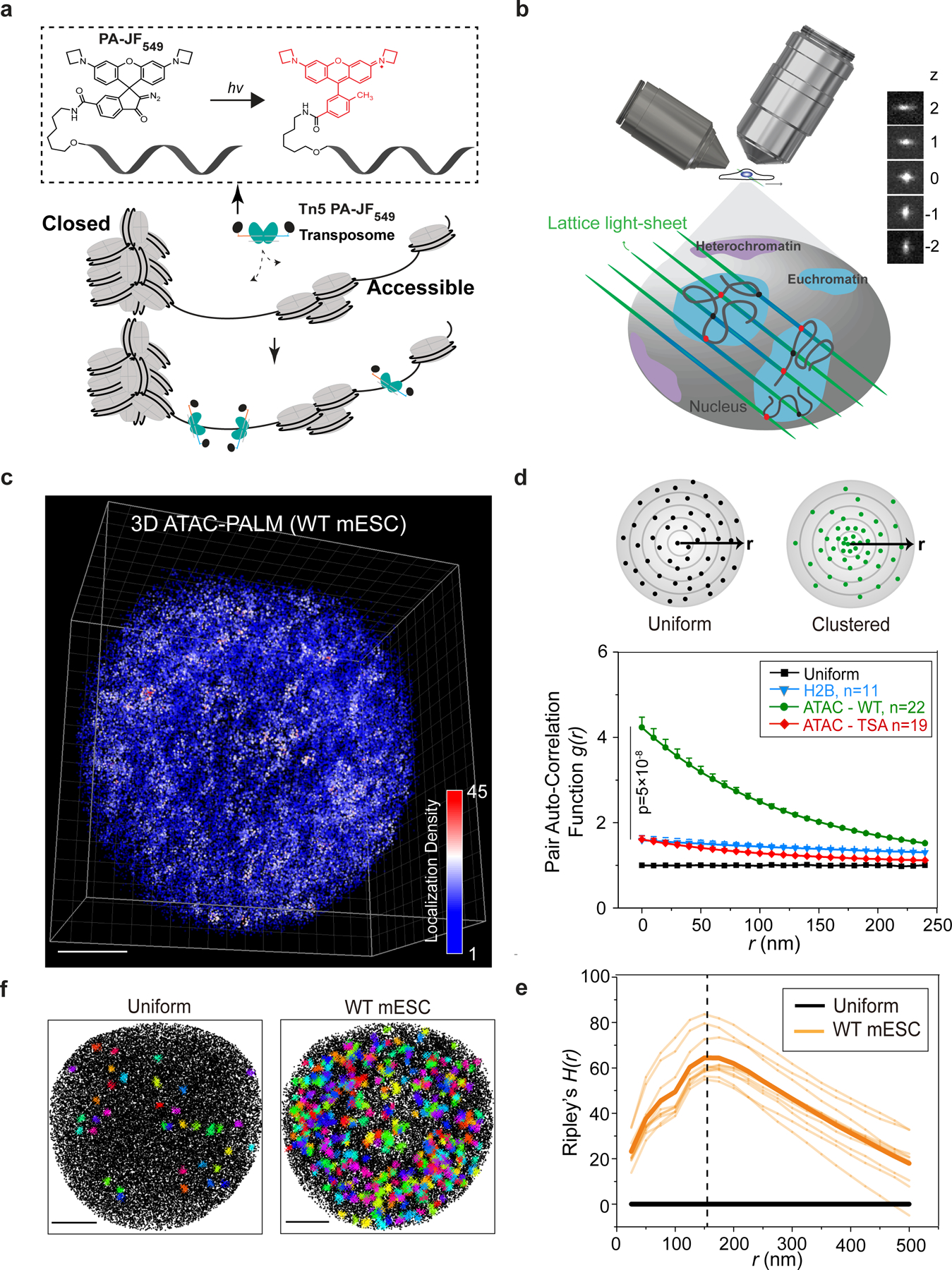
a, Schematics of the 3D ATAC-PALM microscopy labeling and imaging strategy. Photoactivatable Janelia Fluor 549 (PA-JF₅₄₉) was conjugated to DNA oligo containing the mosaic ends of the Tn5 transposon and reconstituted with Tn5 transposase (cyan) to form the active transposome complex in vitro. The cells were fixed, permeabilized, and accessible sites in the genome were selectively labeled by the Tn5 PA-JF₅₄₉ transposome. Photoactivation (hv, 405 nm laser) of the nonfluorescent PA-JF₅₄₉ yields highly fluorescent methyl-substituted JF₅₄₉.

b, Tn5 PA-JF₅₄₉ transposome treated cells were mounted onto the lattice light sheet microscope for 3D ATAC-PALM imaging. A cylindrical lens was introduced to precisely estimate the z coordinates based on the ellipticity of the fluorescent signal. Each z step represents 271 nm distance.

c, 3D illustration of accessible chromatin localizations in wild-type (WT) mouse ESCs. The color-coded localization density was calculated with a canopy radius of 250 nm. A total of n = 22 cells from four biologically independent experiments were imaged with similar results. Scale bar: 2 μm.

d, Global pair auto-correlation function g(r) analysis of ATAC-PALM localizations for WT and TSA treated mESCs. The top panel shows a simplified 2D scheme for uniform (black dots, top left) or clustered (green dots, top right) distribution of localizations. g(r) represents the pair auto-correlation function of distance r calculated from a given origin point within the space. The g(r) for 3D H2B-HaloTag PALM localizations was computed as a control. The error bars represent standard error of the mean (S.E.M). The two-sided non-parametric Mann-Whitney U test was used to compare the clustering amplitude A (equals to g(0)) in different groups. g(r) was plotted from the fitted exponential decay function.

e, Ripley’s H function H(r) of the ACDs from WT mESCs. The black line indicates uniform distribution and the light-yellow lines represent the H(r) from individual WT mESCs (n=10) and the thick yellow line indicate their mean. The vertical dashed line represents the peak radius position around 150 nm.

f, Identification of ACDs by DBSCAN algorithm. Both panels show the Z-projection of all the localizations (black dots) and identified clusters (colored crosses). Left panel, as computational control, DBSCAN only detected 36 clusters in uniformly sampled data points with the same average density as in the right panel. Right panel, DBSCAN identified 402 clusters in WT ESCs in one 3D ATAC-PALM experiment. A total n = 22 cells from 3 biological replicates were used in the analysis. Scale bar, 2 μm.

Statistics source data are provided in Source Data Fig. 1.

To efficiently utilize the photon budget, we performed 3D PALM imaging using the lattice light-sheet microscope¹⁵ with sub-micron illumination thickness to suppress out-of-focus photobleaching and achieve improved signal-to-noise ratio for single-molecule detections throughout the nucleus (Fig. 1b). We also introduced astigmatism with the a cylindrical lens in the detection path^16,17 to generate an axially sensitive point-spread function (PSF) for improved axial localization (z localization precision was improved to ~50 nm) (Fig. 1b). Individual samples were imaged iteratively for at least ~10,000 cycles (~24 hours) to exhaust single-molecule detections. After drift correction, merging consecutive localization events, nucleus segmentation based on a H2B-GFP marker and carefully masking out mitochondrial DNA signals, we obtained 50,000~100,000 effective 3D localizations per nucleus (Extended Data Figure 2a–b). Interestingly, the number of effective localizations detected per nucleus is on the same order of the number of accessible regions identified in bulk and in single-cell ATAC-seq experiments¹¹. More importantly, reducing Tn5 PA-JF₅₄₉ labeling concentrations by 2-fold did not significantly affect the number of effective localizations obtained in individual nuclei (Extended Data Figure 2a), suggesting that the labeling of accessible genomic sites was saturated. We named this super-resolution accessible genome imaging strategy “3D ATAC-PALM”.

It is important to note that only ~2% of the genome is accessible^10–12 and the Tn5 PA-JF₅₄₉ labeling condition (37°C, neutral pH and non-denaturing conditions) is relatively gentle compared to high-temperature, denaturing conditions used in DNA-FISH experiments^18–21. Thus, the ATAC-PALM labeling enabled by probe insertion in a chemically-crosslinked nucleus is unlikely to significantly perturb the overall chromatin structure.

3D ATAC-PALM reveals spatially segregated accessible chromatin domains

After nucleus segmentation and localization-based image reconstruction, we found that accessible genomic regions in mouse ESCs and embryonic fibroblasts (MEFs) are non-homogeneously distributed and organized into spatially segregated 3D clusters. Henceforth, we called these high-density clusters - accessible chromatin domains (ACDs) (Fig. 1c, Supplementary Video 1). To quantify the degree of accessible chromatin clustering, we used the pair auto-correlation function g(r) (Eqn. S8), which was applied by physicists to describe the clustering of stars in galaxies²². g(r) measures the density of localizations on a 3D surface, at a distance of r from the reference point and is equal to 1 for uniformly distributed localizations (Fig. 1d). In our g(r) calculation, we also employed a previously described statistical model²³ to suppress over-counting of single fluorophores due to photo-blinking. We found that the g(r) for ATAC-PALM localizations in both ESCs or differentiated MEFs was significantly higher than that of a uniform distribution at multiple length scales, indicating extensive spatial clustering of accessible chromatin (Fig. 1d and Extended Data Figure 2c). In addition, ATAC-PALM localizations were significantly more clustered than histone H2B PALM localizations collected in the same imaging conditions (Fig. 1d), excluding the possibility that over-counting of blinking molecules could account for 3D clustering of accessible chromatin. We estimated the localization density enrichment at the center of ACDs g(0) by fitting g(r) with a fluctuation model (Eqn. S16) to obtain the clustering amplitude (A) (Fig. 1d). The typical radius of ACDs in wild type ESCs was estimated by using Ripley’s H function H(r) (Eqn. S13). We found that H(r) for ATAC-PALM localizations significantly deviated from a uniform distribution (H(r)=0), reaching a maximum at a radius of ~150 nm (Fig. 1e). Consistent with these results, DBSCAN (Density-Based Spatial Clustering of Applications with Noise)²⁴ analysis identified much larger number (~11 fold more) of ACDs from ATAC-PALM localizations than from uniformly sampled localizations in the same volume (Fig. 1f). It is worth noting that we did not detect significant differences of the g(r) function at distinct interphase stages (e.g. G1, S and G2) demarcated by genetically encoded cell cycle fluorescent reporters (Extended Data Figure 2d–e)²⁵.

To test whether the organization of accessible chromatin can be perturbed, we induced chromatin hyperacetylation by the HDAC inhibitor trichostatin A (TSA)²⁶. TSA treatment markedly reduced g(r) (Fig. 1d), suggesting less clustering and a more homogenous distribution of accessible chromatin in the nucleus. Genome-wide ATAC-seq revealed that TSA treatment not only induced the formation of a large number of new accessible sites in the genome but also reduced chromatin accessibility at enhancer and promoter regions, thus effectively diminishing the contrast of cis-regulatory element landscape in general (Extended Data Figure 2f–g). These results suggested that 3D ATAC-PALM is sufficiently sensitive to detect 3D organizational changes of accessible chromatin.

3D ATAC-PALM multiplexed with Oligopaint DNA-FISH, RNA-FISH and Protein fluorescence

To understand the nature of ACDs, we sought to simultaneously image ACDs and other key features defined from genomic data (e.g. ATAC-seq, ChIP-seq and Hi-C). To this end, we optimized the compatibility of 3D ATAC-PALM with available single-cell imaging techniques such as Oligopaint DNA-FISH, RNA-FISH and protein fluorescence (See detail protocols in Supplementary Methods) (Fig. 2a). For example, by coupling 3D ATAC-PALM with Oligopaint DNA-FISH which employs high-density fluorescent oligo probes to label a particular genomic region^18–21,27, we found that individual ACDs were statistically prone to spatially co-localize with active (ATAC and H3K4me3-rich) genomic regions (Fig. 2b–c, Supplementary Video 2 and 3) and were spatially segregated from inactive (ATAC and H3K4me3-poor) regions (Fig. 2d). Because of the saturated labeling and localization detection in our imaging (Extended Data Figure 2a), the density variation of ATAC-PALM localizations within individual chromatin segments likely reflects the extensive heterogeneity and intrinsic variation of genome folding observed in single cells²⁸ (Fig. 2f). To further investigate whether ACDs are spatially correlated with active chromatin, we coupled 3D ATAC-PALM with RNA-FISH and found that ACDs enclosed an actively transcribed pluripotency marker gene, Nanog (Fig. 2e–f).

Fig. 2 |. ACDs are associated with active chromosomal segments.

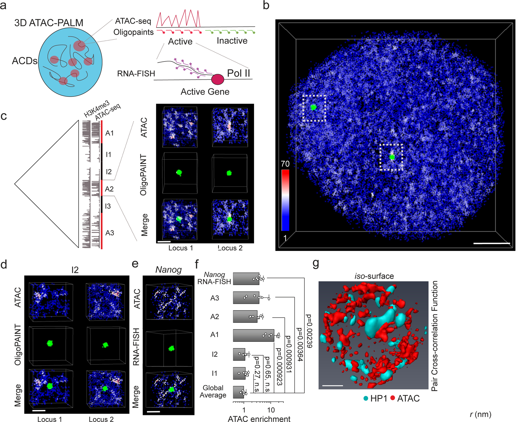
a, Schematics showing multiplexed imaging of 3D ATAC-PALM and Oligopaint DNA-FISH or RNA-FISH.

b, Co-localization of ACDs with ATAC-rich segments. Single-cell illustration of two color imaging of ATAC-PALM (red) and 3D Oligopaint DNA-FISH (green) targeting to an ATAC-rich segment (A2) as shown in the left panel in (c). Scale bar, 2 μm.

c, (Left panel) Alignment of Hi-C heatmap, ATAC-seq and H3K4me3 tracks surrounding the pluripotency gene Nanog on Chromosome 6 (chr6:120080000–125240000). ATAC-rich segments with higher density of ATAC and H3K4me3 peaks are underlined by red bars (A1, A2 and A3). Conversely, low ATAC density and H3K4me3-poor segments are underlined by black bars (I1,I2 and I3). See details of these domain coordinates in the Supplementary Information. (Right panel) Top, zoom-in view of the ACD localizations detected by ATAC-PALM imaging in the active region A2. Middle, the zoom-in view of the Oligopaint DNA-FISH signals of two alleles. Bottom, Zoom-in view showing the colocalization between ACDs and ATAC-rich segments (green) labeled by 3D Oligopaint DNA-FISH probes for both alleles in the cell. Scale bar, 1 μm.

d, ACDs are spatially separated from ATAC-poor segments. Top, Zoom-in view of the ACDs detected by ATAC-PALM imaging. Middle, the zoom-in view of the Oligopaint DNA-FISH signals of two alleles (I2). Bottom, Zoom-in view shows spatial separation of ACDs from ATAC-poor segments (green) labeled by 3D Oligopaint DNA-FISH probes for both alleles in the cell. Scale bar, 1 μm.

e, ACDs enclose actively transcribed gene Nanog. Top, Zoom-in view of the ACDs detected by ATAC-PALM imaging. Middle, the zoom-in view of the RNA-FISH signals of the Nanog gene (A2 region) using intronic probes marking the transcription site. Bottom, Zoom-in view shows that the actively transcribed Nanog gene is enclosed within the high density accessible chromatin region. Representative images in Fig. b-e are from two biologically independent experiments with similar results. Scale bar, 1 μm.

f, ATAC-PALM localizations were significantly enriched in ATAC-rich segments (A1,A2 and A3) labeled by 3D Oligopaint DNA-FISH probes and in actively transcribed regions (Nanog RNA-FISH) but not in ATAC-poor segments (I1 and I2). Specifically, the plot represents the log scale fold enrichment for ATAC-PALM localizations in the DNA-FISH or RNA-FISH labeled regions over the average density in the nucleus. The error bar represents SD. Each dot represents one analyzed locus for each condition. Statistical tests were performed by using two-sided non-parametric Mann-Whitney U test.

g, ACDs are spatially segregated from heterochromatic regions. Left, 3D spatial relationship between accessible chromatin (red, Gaussian blurred) and heterochromatin (turquoise, HP1α-GFP). Scale bar: 2 μm. Right, 2D pair cross-correlation function calculated for accessible chromatin (red) and heterochromatin (turquoise) regions. The curve represents the mean of pair cross-correlation function values across 2D slices from n = 10 cells and the error bars represent S.E.M.

Statistics source data are provided in Source Data Fig. 2.

To overcome the specificity and resolution limitation of antibody based imaging, we generated genome-edited mESC lines in which we fused the HaloTag to endogenous regulatory proteins associated with active chromatin (e.g. histone variant H2A.Z and Mediator subunit 1(MED1))^29,30. After accessible chromatin and HaloTag labeling with photoactivatable Janelia Fluor 549 and 646¹³ respectively, we performed two-color, super-resolution 3D PALM imaging. Pair cross-correlation analysis revealed that localizations of H2A.Z or MED1 were spatially correlated with ATAC localizations across multiple scales (Extended Data Figure3). In contrast, ACDs and HP1-GFP labeled heterochromatic regions were mutually exclusive, organized into distinct salt-and-pepper spatial patterns in the nucleus (Fig. 2g, Supplementary Video 4). Taken together, these results validated that ACDs revealed by 3D ATAC-PALM represent structures of active, accessible chromatin that are spatially segregated from heterochromatin. Meanwhile, we also demonstrated that 3D ATAC-PALM can be coupled with other single-cell imaging techniques (such as Oligopaint DNA-FISH, RNA-FISH, protein fluorescence-based super-resolution imaging) to study genome organization.

CTCF prevents excessive clustering of accessible chromatin

To further understand the mechanism underlying the spatial organization of ACDs, we focused on genome architectural protein CTCF³¹. To deplete CTCF with minimal secondary effects, we employed the auxin-inducible degron (AID) system³² and tagged endogenous CTCF with a HaloTag-miniAID (mAID) in a mESC line stably expressing the rice F-box protein TIR1 (Fig. 3a). The HaloTag-mAID was fused to the N-terminus of CTCF to avoid previously reported problems (e.g. auxin independent degradation and interference with CTCF function) associated with C-terminal tagging³³. We found that HaloTag-mAID labeling of CTCF influenced neither basal protein levels (Extended Data Figure 4a) nor cell proliferation before auxin treatment (Extended Data Figure4e–g). Within a few hours of auxin treatment, CTCF expression was undetectable by western blot, single-cell fluorescence imaging or flow cytometry (> 99% depletion) (Fig. 3a, Extended Data Figure 4a–d). The depletion was reversible, as CTCF protein levels quickly recovered after auxin washout (Extended Data Figure 4d). Acute loss of CTCF (up to 12 hours) did not cause noticeable changes in proliferation, cell cycle phasing or expression of pluripotency markers (Fig. 3a, Extended Data Figure 4a, c, e–g), although prolonged CTCF (> 48 hours) loss did compromise proliferation, colony formation and survival of ESCs (Extended Data Figure 4e–g).

Fig. 3 |. Structural variation of accessible chromatin upon acute loss of CTCF.

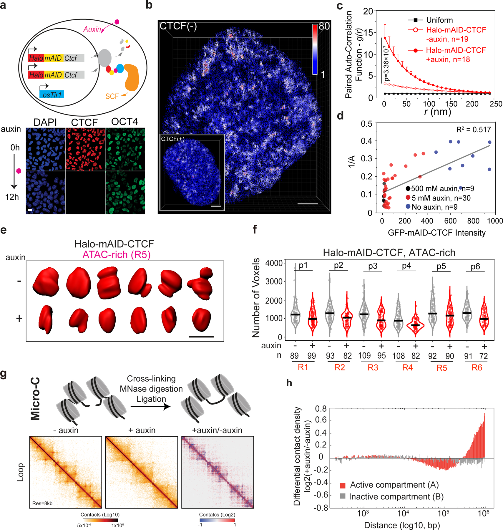
a, Acute depletion of CTCF in mESCs by the auxin-induced degradation system. The mini auxin-inducible degron (mAID)-HaloTag (Halo) was bi-allelically knocked into the N-terminus of Ctcf by CRISPR/Cas9 genome editing technology (upper panel) in a mouse ESC line stably expressing the plant E3 ligase adaptor protein osTir1. Adding auxin analogue triggers rapid degradation of target protein CTCF revealed by immunofluorescence (lower panel). OCT4 immunostaining was used as a control. n = 2 biological replicates. Scale bar, 5 μm.

b, Single-cell 3D illustration of ATAC-PALM localizations upon CTCF depletion (CTCF(−)). The Inset shows 3D ATAC-PALM localizations of a cell without CTCF depletion (CTCF(+)) for comparison. The color bar indicates localization density calculated by using a canopy radius of 250 nm. For the CTCF(+) condition, The inset panel used the localization density bar scaling from 1 to 50. The average localization density is the same for both cells. Experiments were repeated 3 times with similar results. Scale bar, 2 μm.

c, CTCF depletion promotes global accessible chromatin clustering. The error bar represents S.E.M and two-sided Mann-Whitney U test was applied for comparing data points at g(0).

d, The dose-dependent effect of CTCF depletion on global accessible chromatin clustering revealed by the inverse relationship between clustering amplitude (A) and residual CTCF levels measured by GFP-mAID-CTCF fluorescence intensities (arbitrary fluorescent units). A linear regression model was applied to derive the correlation of determination R².

e, Representative iso-surfaces of an ATAC-rich segment (R5, red) before (−) and after (+) CTCF depletion (12 hours). Scale bar, 1 μm. Representatives images are from n = 3 biological replicates with similar results.

f, Violin plot of 3D volumes (the number of voxels) of six ATAC-rich segments (R1–R6) before and after CTCF depletion. Throughout the volume measurements in this study, each voxel size is x=48.9 nm, y=48.9 nm, z=199 nm. The number of alleles analyzed is indicated at the bottom. The black bar indicates the median value for each data set and two-sided Mann-Whitney U test was applied for statistical test. P-values for R1–R6 are: p1=0.00839, p2=1.17×10⁻⁶, p3=6.26×10⁻⁶, p4=4.97×10⁻⁷, p5=0.00166, p6=2.51×10⁻⁶.

g, Top panel, schematic of the high-resolution Micro-C experiment. Lower panel, snapshots of Micro-C contact maps in auxin-mediated CTCF depletion (6 hours) cells on chr1:132.5M-134.5M at 8-kb resolution. Contact matrixes and differential contact maps showed loss of loops after CTCF depletion.

h, Differential contact probability in compartment A and B. Differential contact probability was calculated by dividing the genome-wide decaying curve of CTCF depletion condition (+auxin) over non-depleted control (-auxin). Compartment A showed a much greater magnitude of changes in contact frequency at a distance between 25kb to 1Mb than that in compartment B.

Statistics source data are provided in Source Data Fig. 3.

Acute loss of CTCF triggered prominent organizational changes in ACDs (Fig. 3b, Supplementary Video 5) and markedly enhanced accessible chromatin clustering as the g(r) function increased significantly across multiple length scales relative to unperturbed conditions (Fig. 3c). We found that, at the single cell level, the efficiency of CTCF depletion was positively correlated with the degree of accessible chromatin clustering (1/A, equals to 1/g(0)) (Fig. 3d). Furthermore, the increase in accessible chromatin clustering induced by CTCF depletion was largely reversed when CTCF levels recovered after auxin washout (Extended Data Figure 5a). As a control, genome-wide ATAC-seq revealed that acute loss of CTCF did not significantly affect chromatin accessibility at enhancers and promoters, although chromatin accessibility at CTCF binding sites was reduced (Extended Data Figure 5b–c, Extended Data Figure 5d–f). Consistent with these results, DBSCAN analysis revealed higher ATAC localization densities within individual ACDs (Extended Data Figure 5g–h), suggesting that CTCF might regulate compaction of accessible chromatin.

CTCF decompacts ACDs

To investigate the link between CTCF and chromatin compaction, we labeled 6 active and 5 inactive chromosomal segments that were well-demarcated based on chromatin accessibility and CTCF binding with high density Oligopaint FISH probes (Extended Data Figure 6a–b). We measured the 3D volume for each segment after iso-surface based segmentation of Airyscan images (Supplementary Video 6). We found that, after length normalization, active segments generally occupied larger volumes relative to inactive segments (Extended Data Figure 6c), in good agreement with previously published STORM imaging results²⁰. Consistent with the increased clustering and higher localization density of accessible chromatin within ACDs, 3D volumes of active segments were significantly reduced, whereas inactive segments appeared largely unaffected upon CTCF depletion (Fig. 3e–f, Extended Data Figure 6d–e).

To further validate our single-cell imaging data, we performed high resolution Micro-C experiments after acute CTCF depletion (6 hours) in ESCs^34,35 (Fig. 3g). Consistent with previous Hi-C results³¹, we found that the number of chromatin loops and that of TADs were significantly reduced after CTCF loss whereas A/B compartments remained largely intact (Fig. 3g, Extended Data Figure 7, Fig. 8). Notably, CTCF depletion significantly enhanced contact probabilities within active chromatin segments but not within inactive ones (Fig. 3f), in good agreement with our 3D ATAC-PALM and Oligopaint DNA-FISH imaging data that CTCF depletion enhanced accessible chromatin clustering and compacted ACDs. These results are also consistent with predictions from the proposed loop extrusion model^36–38. Specifically, without adequate insulation by CTCF, Cohesin continues to extrude chromatin DNA, resulting in compaction of accessible chromatin. However, due to the lack of CTCF binding at inactive (ATAC-poor) regions, CTCF depletion would not induce chromatin compaction at these regions just as what we observed here (Fig. 3h, Extended Data Figure 6d–e). Thus, in addition to providing supportive evidence to previous modeling predictions based on Hi-C genomic data^31,37,39, these single-cell imaging results further underscored the potential of 3D ATAC-PALM as a tool to probe genome organization.

Discussion

Here we demonstrated that 3D ATAC-PALM enables super-resolution in situ imaging of the spatial organization of the accessible genome in different cell types of interest. 3D ATAC-PALM imaging in formaldehyde fixed cells makes it potentially applicable to formalin fixed tissue slices and other clinical samples. The compatibility of 3D ATAC-PALM with Oligopaint DNA-FISH, RNA-FISH, and protein fluorescent imaging makes this method readily adaptable to researchers from a wide range of biomedical fields. We have demonstrated that 3D ATAC-PALM exhibits exquisite sensitivity to detect the spatial organizational changes of genome topology under a variety of chemical-genetic perturbations (TSA, CTCF depletion et al), which are further validated by orthogonal approaches (Oligopaint DNA-FISH or Micro-C). We envision that this new single-cell super-resolution imaging method will complement existing genome imaging (DNA-FISH, CRISPR imaging et al.) and sequencing (Hi-C et al.) methods to understand fundamental principles underlying the 3D genome organization in situ.

The clustering of accessible chromatin unveiled by 3D ATAC-PALM highlights the prevalent spatial proximity among cis-regulatory elements, reminiscent of the extensive promoter-promoter, enhancer-enhancer and enhancer-promoter interactions captured by ensemble chromatin interaction experiments^40,41. The architecture of clustered cis-regulatory elements may thus serve as a topological basis for mediating long-range enhancer-promoter communications and precise spatiotemporal gene expression control. In the future, high-throughput, sequence-specific Oligopaint DNA-FISH-based barcoding strategies^27,42,43 in combination with 3D ATAC-PALM may help delineate the spatial relationship between ACDs, compartments, TADs and loops and the architectural basis of gene regulation. Integrating 3D ATAC-PALM with other functional (epi)genomic, genome editing, and live cell imaging approaches will faciliate dissecting funadmental mechanisms and functions of the spatial organization of the accessible genome. ATAC-seq has been applied to profile the human cancer landscape and enables classification of cancer subtypes with important prognostic value⁴⁴. It will be of practical interest to unleash the exquisite spatial resolution of 3D ATAC-PALM to examine the accessible genomic landscape in disease specimens for clinical diagnosis and mechanistic investigations.

Methods:

Tn5 Expression and Purification

The plasmid pTXB1-Tn5 (Addgene #60240) was used to express the hyperactive Tn5 transposase fused with the Mxe Intein and Chitin-binding domain⁴⁵. Briefly, the pTXB1-Tn5 was transformed into the T7 Express lysY/Iq Competent E. coli (NEB, cat# C3013I). 1 litter culture of transformed cells were grown in TB buffer with antibiotics at 37°C to A₆₀₀ ~0.6 and induced with 0.25 mM IPTG. The cells were incubated at 23°C for 4 h, harvested, and washed with 50 mL 1× PBS with cOmplete™ Protease Inhibitor Cocktail (Roche). The cell pellet was snap frozen in liquid nitrogen, stored at −80°C overnight, resuspended in 160 mL HEGX (20 mM HEPES-KOH at pH 7.2, 0.8 M NaCl, 1 mM EDTA, 10% glycerol, 0.2% Triton X-100) with Protease Inhibitor and sonicated for 10 cycles of 30s ON/60s OFF at 30 W output on a Model 100 Sonic Dismembrator (Fisher Scientific). The lysate was centrifuged in a Beckman JA25.50 rotor at 16,000 rpm for 30 min at 4°C and 8.4 mL 5% neutralized PEI (Sigma P3143) was added dropwise into the supernatant with gentle agitation for 15 minutes at 4°C followed by another centrifuge at 13,000 rpm for 10 min at 4°C. Meantime 20 mL Chitin Resin (NEB cat#S6651L) was equilibrated in a column with 200mL of HEGX buffer supplemented with protease inhibitor and loaded with the supernatant from the PEI-centrifuge step by slow gravity flow (<0.3mL/min). The column was washed with 400 mL HEGX overnight at a flow rate ~0.6 mL/min. To cleave the Tn5 from the Intein, 48 mL HEGX buffer + 100 mM DTT supplemented with protease inhibitor was loaded to the top of the column bed and the column was left closed for 48 h at 4° C. Cleaved Tn5 was eluted in ~1 mL fractions and Tn5 elution efficiency was monitored by the Pierce™ Coomassie (Bradford) Protein Assay Kit (Thermo Fisher Scientific cat# 23200). Fractions with the strongest absorbance were pooled and dialyzed versus two changes of 2 L of 2X Tn5 dialysis buffer (100 mM HEPES-KOH at pH 7.2, 0.2 M NaCl, 0.2 mM EDTA, 2 mM DTT, 0.2% Triton X-100, 20% glycerol) at 4° C. After dialysis, the protein concentration was measured using a Nanodrop spectrophotometer (Thermo Scientific) and confirmed by running an SDS-PAGE gel using BSA as a standard. Tn5 protein was further concentrated to 20 mg/mL using the Amicon Ultra-15 Centrifugal Filter Unit and we added 50% glycerol to the final concentrate and prepared aliquots in screw-top microcentrifuge tubes, flash freeze in liquid nitrogen, and store at −80° C. The Tn5 activity was tested by the in vitro tagmentation assay⁴⁵ and further verified by performing genome wide ATAC-seq experiment.

PA-JF₅₄₉ dye-oligo conjugation and purification

The mosaic ends (ME) adaptors for Tn5 transposase were synthesized by Integrated DNA Technologies (IDT) with attachment of a 5’ end primary amino group by a six-carbon spacer arm (C6). The oligonucleotide sequences and their modifications are:

Tn5ME-A: 5′-amino-C6 TCGTCGGCAGCGTCAGATGTGTATAAGAGACAG3′

Tn5ME-B: 5′-amino-C6-GTCTCGTGGGCTCGGAGATGTGTATAAGAGACAG-3′

Tn5MErev: 5′-[phos]CTGTCTCTTATACACATCT-3′

The photoactivatable Janelia Fluor 549 coupled to the N-hydroxysuccinimide (NHS) ester (NHS-PA-JF₅₄₉) was synthesized by the Luke Lavis’s group at Janelia Research Campus. The NHS-PA-JF₅₄₉ was dissolved in anhydrous dimethylsulfoxide (DMSO) immediately before conjugation. The Tn5ME-A and Tn5ME-B oligos were first dissolved in deionized water and then extracted three times with chloroform. The upper aqueous solution was carefully extracted and precipitated by 3M sodium acetate (pH 5.2) and ethanol. The pellet was washed with 70% ethanol, dried and dissolved in ultrapure water. The purified oligos were reacted with excessive NHS-PA-JF₅₄₉ in anhydrous DMSO (mass ratio 1:2.5) in the labeling buffer (0.1 M sodium tetraborate, pH 8.5). The reaction was incubated at room temperature for overnight (>12 hours) with constant stirring and protection from light. The conjugation reaction was further precipitated by 3M sodium acetate, pH 5.2 and ethanol. The purified pellet was dissolved in 0.1 M TEAA (triethylammonium acetate) (Thermo Fisher Scientific cat# 400613).

Purification of oligo-dye conjugates were performed on Agilent 1200 Analytical HPLC system equipped with an autosampler, diode array detector and fraction collector. The column used was Eclipse XDB-C18 column (4.6 × 150 mm 5 μm, Agilent) and eluted with a linear gradient of 0–100% MeCN/H₂O with constant 10 mM TEAA additive; 30 min run; 1ml/min flow, detection at 260 nm. Sample fractions were pooled and lyophilized to obtain the product as white solid.

In vitro Tn5 transposome assembly, validation and preparation for PALM imaging

The HPLC purified Tn5ME-A-PA-JF₅₄₉, Tn5ME-B-PA-JF₅₄₉, Tn5MErev oligos were resuspended in water to 100 μM each. Tn5ME-A-PA-JF₅₄₉ or Tn5ME-B-PA-JF₅₄₉ were mixed with Tn5MERev in each molar ratio in 1X annealing buffer (10mM Tris HCl pH8.0, 50mM NaCl, 1mM EDTA) and were denatured on a benchtop thermocycler at 95 °C for 5 min and then slowly cooled down to 25°C at the rate of −1°C /min. We assembled the Tn5 transposome with PA-JF₅₄₉ according to previously published protocol¹² by combining 0.25 vol Tn5MErev/Tn5ME-A-PA-JF₅₄₉ + Tn5MErev/Tn5ME-B-PA- JF₅₄₉ (50 μM each), 0.4 vol glycerol (100% solution), 0.12 vol 2× dialysis buffer (100 mM HEPES–KOH at pH 7.2, 0.2 M NaCl, 0.2 mM EDTA, 2 mM DTT, 0.2% Triton X-100, 20% glycerol), 0.1 vol Tn5 (50 μM), 0.13 vol H2O, followed by gentle nutation at room temperature for 1 hour. The activity of in-house prepared Tn5 transposome was validated by genome-wide ATAC-seq as described previously¹² following an reverse crosslinking step.

We prepared cells for 3D ATAC-PALM experiments as reported previously¹². Briefly, cells (mouse ESC or MEF) were plated onto #1 thickness 5mm coverslips (Warner Instruments, cat#64–0700) at around 70–80% confluency with proper coating one day before experiment. Cells were fixed with 1% paraformaldehyde (Electron Microscopy Sciences, Cat# 15710) for 10 min at room temperature. After fixation, cells were washed three times with 1 X PBS for 5 minutes and then permeabilized with ATAC lysis buffer (10 mM Tris–Cl, pH 7.4, 10 mM NaCl, 3 mM MgCl2, 0.1% Igepal CA-630) for 10 min at room temperature. After permeabilization, the slides were washed twice in 1XPBS and put inside a humidity chamber box at 37 °C. The transposase mixture solution (1× Tagmentation buffer-10mM Tris-HCl, pH 7.6, 5mM MgCl2, 10% dimethylformamide, 100 nM Tn5- PA-JF₅₄₉) was added to the cells and incubated for 30 min at 37 °C inside the humidity chamber. After the transposase reaction, slides were washed three times with 1 X PBS containing 0.01% SDS and 50 mM EDTA for 15 min at 55 °C before mounted onto the Lattice light-sheet microscope (LLSM) slot for 3D ATAC-PALM imaging.

3D ATAC-PALM image acquisition and processing

The 3D ATAC-PALM data were acquired by the Lattice light-sheet microscopy¹⁵ at room temperature. The light sheet was generated from the interference of highly parallel beams in a square lattice and dithered to create a uniform excitation sheet. The inner and outer numerical apertures of the excitation sheet were set to be 0.44 and 0.55, respectively. A Variable-Flow Peristaltic Pump (Thermo Fisher Scientific) was used to connect a 2L reservoir with the imaging chamber with 1×PBS circulating through at a constant flow rate. Labelled cells seeded on 5mm coverslips (Warner Instruments) were placed into the imaging chamber and each image volume includes ~100–200 image frames, depending on the depth of field of view. Specifically, spontaneously activated PA-JF₅₄₉ dye were initially pushed into the fluorescent dark state through repeated photo-bleaching by scanning the whole image view with a 2W 560 nm laser (MPB Communications Inc., Canada). Then, the samples were imaged by iteratively photo-activating each plane with very low intensity 405 nm light (<0.05 mW power at the rear aperture of the excitation objective and 6W/cm² power at the sample) for 8 ms and by exciting each plane with a 2W 560 nm laser at its full power (26 mW power at the rear aperture of the excitation objective and 3466 W/cm² power at the sample) for 20 ms exposure time. The specimen was illuminated when laser light went through a custom 0.65 NA excitation objective (Special Optics, Wharton, NJ) and the fluorescence generated within the specimen was collected by a detection objective (CFI Apo LWD 25×W, 1.1 NA, Nikon), filtered through a 440/521/607/700 nm BrightLine quad-band bandpass filter (Semrock) and N-BK7 Mounted Plano-Convex Round cylindrical lens (f = 1000 mm, Ø 1”, Thorlabs), and eventually recorded by an ORCA-Flash 4.0 sCMOS camera (Hamamatsu). The cells were imaged under sample scanning mode and the dithered light sheet at 500 nm step size, thereby capturing a volume of ~25 μm × 51 μm × (27~54) μm, considering 32.8° angle between the excitation direction and the stage moving plane. All measurements were taken from distinct cells.

To precisely analyze the 3D ATAC-PALM data, we embedded nano-gold fiducials within the coverslips for drift correction as previously described¹⁶. ATAC-PALM Images were taken to construct a 3D volume when the sample was moving along the “s” axis. Individual volumes per acquisition were automatically stored as Tiff stacks, which were then analyzed by in-house scripts written in Matlab. The cylindrical lens introduced astigmatism in the detection path and recorded each isolated single molecule with its ellipticity, thereby encoding the 3D position of each molecule relative to the microscope focal plane. All processing was performed by converting all dimensions to units of xy pixels, which were 100 nm × 100 nm after transformation due to the magnification of the detection objective and tube lens. We estimated the localization precision by calculating the standard deviation of all the localizations coordinates (x, y and z) after the nano-gold fiducial correction. The localization precision is 26±3 nm and 53±5 nm for xy and z, respectively.

Raw 3D ATAC-PALM images were processed following previous published procedures^15,16. Specifically, a background image with gray values taken without illumination was subtracted from each frame of the current raw image. Photo-activated images were then filtered by subtracting Gaussian filtered images at two different standards:

$${\mathrm{I}}_{\mathit{\text{filtered}}}={\mathrm{I}}_{raw}\otimes K_{low}-{\mathrm{I}}_{raw}\otimes K_{\mathit{\text{high}}}$$ (Equation S1)

Where ⊗ is the convolution operator, and K_low and K_high represent 5×5 pixel two-dimensional Gaussian function with standard deviation σ=2 (low) and 1 (high):

$$K=2{\pi }^{-3/2}{\sigma }^{-2}\cdot e^{-\frac{{(x-3)}^2}{2{\sigma }^2}-\frac{{(y-3)}^2}{2{\sigma }^2}}$$ (Equation S2)

The local maxima were then determined on these filtered images and the coordinates were estimated and used as the true position of the isolated single molecule.

In order to precisely determine the z position of each isolated localization, cylindrical lens were used and the corresponding astigmatic PSF function could be formulated as a Gaussian function with separate x and y deviations. Importantly, these deviations encoded the relative z-offset of the signal with respect to the focal plane.

$$PSF(x,y,z)=\frac{1}{2\pi {\sigma }_x{\sigma }_y}\cdot e^{-\left(\frac{x^2}{2{\sigma }_x^2}+\frac{y^2}{2{\sigma }_y^2}\right)}$$ (Equation S3)

Where

$${\sigma }_x=c_1+c_{2}z+c_3{z}^2$$

$${\sigma }_y=c_4+c_{5}z+c_6{z}^2$$

Here σ_x and σ_y were polynomial function of z. The constants c₁~c₆ can be fitted by scanning bright and regular beads through the focal plane using piezoelectric stage.

To rigorously compare ATAC-PALM localizations within the nucleus, image stack for H2B-GFP stably expressed in mouse ESCs was captured before the ATAC-PALM experiment under the same Lattice light-sheet Microscopy imaging condition. The image stack of the GFP channel was de-skewed and de-convoluted using the same algorithm to identify a nuclear mask to segment ATAC-PALM signal. The percentage of localizations falling into the same volume in or out of the mask were counted and plotted in Figure S2B. We found that the majority (>95%) of localizations fall into the nuclear H2B mask, suggesting that the manual segmentation based on ATAC-PALM signal intensity is sufficient to distinguish it from out-of-nucleus signal (e.g. mitochondria) or non-specific background.

To derive the ATAC-PALM intensity map in order to compare with HP1-GFP labeled heterochromatin spatial distribution, ATAC-PALM localizations were binned within a cubic of 100 nm with a 3D Gaussian filter and a convolution kernel of 3×3×3.

3D pair auto-correlation function, pair cross-correlation function and Ripley’s function

As described previously⁴⁶, the pair correlation function g₀(r) or radial distribution function measures the probability P of finding a localization of accessible chromatin in a volume element dV at a separation r from another accessible chromatin site:

$$P=\rho \cdot g_0(r)\cdot dV$$ (Equation S5)

Where ρ represents the mean density of accessible chromatin in the nucleus.

3D g₀(r) was computed by

$$g_0(r)=\frac{3V}{4\pi (3r^2\cdot \Delta r+3r\cdot \Delta r^2+\Delta r^3)}\cdot \frac{1}{N\cdot (N-1)}\sum _{i=1}^N\sum _{i\ne j}\delta (r-r_{ij})$$ (Equation S6)

N is the total number of localizations and V is the 3D nuclear volume. Δr = 50 nm is the binning width used in the analysis. The item 4π(3r²·Δr + 3r·Δr² + Δr³)/3 represents the shell-shape volume between the search radius from r to r + Δr. The Dirac Delta function is defined by

$$\delta (r-r_{ij})=\{\begin{array}{c}\begin{array}{cc}1& r-r_{ij}\le \Delta r\end{array}\\ \begin{array}{cc}0& r-r_{ij}>\Delta r\end{array}\end{array}$$ (Equation S7)

Where r_ij represents the pair-wise Euclidean distance between localization point i and j. To eliminate the boundary effect in calculation of g₀(r) from a finite 3D volume, we generated g_r(r) from uniform distributions with the same localization density in the same volume as real data using the Matlab convex hull function. Accordingly, the final normalized 3D pair auto-correlation function G(r) was calculated by:

$$G(r)=\frac{g_0(r)}{g_r(r)}$$ (Equation S8)

Similarly, the 3D pair cross-correlation function c₀(r) between localizations of molecule A and those of molecule B can be formulated as

$$c_0(r)=\frac{3V}{4\pi (3r^2\cdot \Delta r+3r\cdot \Delta r^2+\Delta r^3)}\cdot \frac{1}{M\cdot N}\sum _{i=1}^M\sum _{j=1}^N\delta (r-r_{ij})$$ (Equation S9)

M is the total number of localizations for molecule A and N is the total number of localizations for molecule B. The Dirac Delta function is defined as the same as in Equation S7. Similarly, the final normalized 3D pair auto-correlation function C(r) was calculated by:

$$C(r)=\frac{c_0(r)}{c_r(r)}$$ (Equation S10)

c_r(r) refers to the pair cross-correlation function calculated from uniform distributions with the same localization density in the same volume as real data used.

Ripley’s K function is a variation of pair correlation function to study point distribution patterns and is defined by the equation:

$$K(r)=\frac{V}{N-1}\left[\frac{1}{N}\sum _{i=1}^N\sum _{i\ne j}{\delta }_K(r-r_{ij})\right]$$ (Equation S11)

where its Delta function given by

$${\delta }_K(r-r_{ij})=\{\begin{array}{c}\begin{array}{cc}1& r-r_{ij}\le 0\end{array}\\ \begin{array}{cc}0& r-r_{ij}>0\end{array}\end{array}$$

The K(r) for a random Poisson distribution is πr². Therefore, its derivative Ripley’s L function is given by

$$L(r)=\sqrt{\frac{K(r)}{\pi }}$$ (Equation S12)

The deviation of L(r) from expected random Poisson distribution can be used to indicate point clustering or dispersion. The further normalized Ripley’s H function

$$H(r)=L(r)-r$$ (Equation S13)

Can be used to estimate the point clustering and domain size⁴⁷.

Whereas G(r) can be used as bona fide criteria for estimating the clustering effect of a group of spatial localizations, it has to be adjusted regarding the inevitable localization uncertainty of the PSF. If the distribution is purely random, the revised pair auto-correlation G_R(r) considering PSF uncertainty is given by

$$G_R(r)=G_{PSF}(r)+1$$ (Equation S14)

with

$$G_{PSF}(r)=\frac{1}{8{\pi }^{3/2}{\sigma }^3}{e}^{-r^2/4{\sigma }^2}$$ (Equation S15)

where ρ represents the average surface density of molecules, G_PSF(r) denotes the correlation of uncertainty in the PSF and σ for standard deviation. The spatial autocorrelation of accessible chromatin can be approximated by an exponential function:

$$g(r)=A\cdot e^{-r/\epsilon }+1$$ (Equation S16)

where ε and A denotes the correlation length and amplitude of the accessible chromatin cluster, respectively. The total correlation can be described by

$$G(r)=G_{PSF}(r)+\left(A\cdot e^{-r/\epsilon }+1\right)\otimes G_{PSF}(r)$$ (Equation S17)

The raw data were fitted by using Equation S17 to derive g(r) and parameters A and ε. The approximated function g(r) was used throughout the paper for pair auto-correlation analysis. Curve fitting was performed using the trust-region method implemented in the Curve Fitting Matlab toolbox.

Since over-counting does not give rise to apparent co-clustering in double label experiments when pair cross-correlation functions are measured⁴⁸, C(r) can serve as bona fide criteria for estimating the co-clustering effect of spatial localizations from two different channels without additional adjustment.

2D pair cross-correlation function and auto-correlation function

To calculate the spatial cross-correlation between the two-color ATAC localization signal and the heterochromatin HP1α signal, we first converted the localization densities into intensity map via 2D Gaussian blurring. The pair cross-correlation function $c(\overrightarrow{r})$ was then calculated by the fast Fourier transform (FFT) method described previously⁴⁶.

$$c(\overrightarrow{r})=\text{Re}\left\{\frac{FF{T}^{-1}(FFT(I_1)\times \mathit{\text{conj}}[FFT(I_2)])}{{\rho }_1{\rho }_{2}N(\overrightarrow{r})}\right\}$$ (Equation S18)

$$N(\overrightarrow{r})=FF{T}^{-1}({|FFT(\mathit{\text{Mask}})|}^2)$$ (Equation S19)

The $N(\overrightarrow{r})$ is the auto-correlation of a mask matrix that has the value of 1 inside the nucleus used for normalization. Conj[] refers to complex conjugate, ρ₁ and ρ₂ are the average surface densities (number of localizations divided by the surface area) of images I₁ and I₂, and Re{} indicates the real part. The fast Fourier transform and its inverse (FFT and FFT⁻¹) were computed by fft2() and ifft2() functions in Matlab, respectively. Cross correlation functions were calculated first by converting the Cartesian coordinates to polar coordinates by Matlab cart2pol() function, binning by radius and by averaging within the assigned bins.

DBSCAN analysis

The density-based clustering algorithm DBSCAN (Density-Based Spatial Clustering of Applications with Noise) was adopted to map and visualize individual local ACDs (core DBSCAN Matlab code from http://yarpiz.com/255/ypml110-dbscan-clustering). The algorithm first finds neighboring data points within a sphere of radius r, and adds them into same group. In parallel, a predefined threshold minimal points (minPts) was used by the algorithm to justify whether any counted group is a cluster. If the number of points within a group is less than the threshold minPts, the data point is classified as noise. As a negative control, we generated uniformly sampled data sets with the same localization density as our ATAC-PALM localizations. We then implemented DBSCAN analysis by using 150 nm as the searching radius (r) (peak radius from the Ripley’s H function analysis) and empirically setting minPts as 10. To reconstruct the iso-surface for each identified ACD, the convex hull which contains the ACD data points was calculated and visualized by using Matlab. The volume of the convex hull was computed, and the normalized cluster radius (calculated from a sphere with equal volume) was estimated and shown in violin plot.

Additional methods involved in this study are included in the Supplementary Note.

Statistical Analysis

Statistical analysis was performed using Origin and GraphPad Prism. Unless stated specifically, data are presented as Mean ± SEM (standard error) with statistical significance (* p < 0.05, ** p < 0.01, *** p <0.001, with the exact p values in the Figure legends). All values of n are provided in the Figure legends. We used non-parametric two-tailed Mann-Whitney U tests unless indicated in the Figure legends.

Extended Data

Extended Data Figure 1 |. 3D ATAC-PALM labeling strategy.

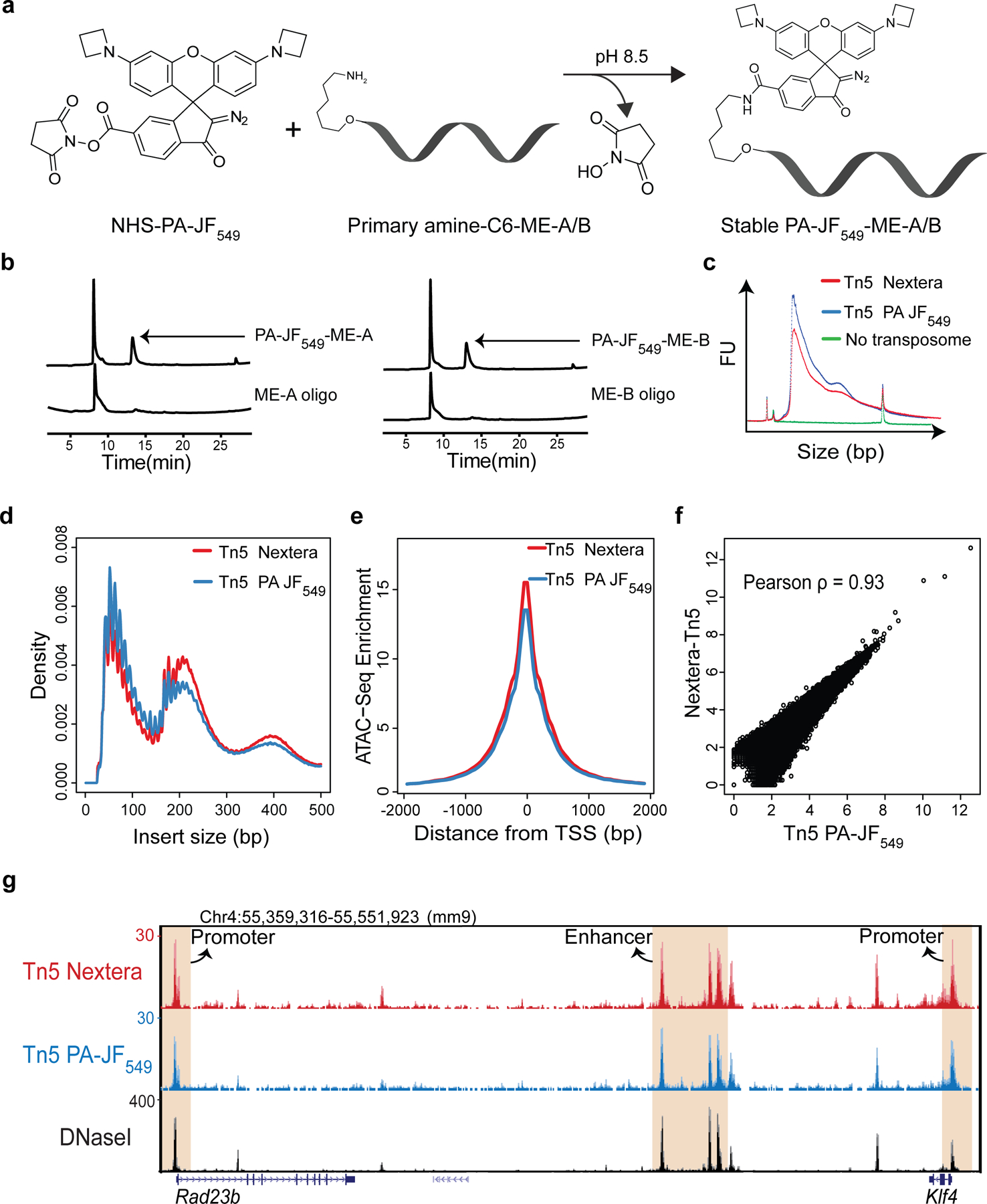
a, N-hydroxysuccinimide (NHS) ester chemical conjugation chemistry. PA-JF₅₄₉ dye coupled with the NHS ester reacts with the primary amine group on the Tn5 ME oligos to yield the stable dye-oligo conjugate via the covalent amide bond.

b, The chromatogram of PA-JF₅₄₉ NHS ester and oligo amine reaction by reverse phase High Pressure Liquid Chromatography (HPLC). The oligo-dye stable conjugates (smaller peaks as indicated by arrows) were selectively purified. Representative image from n = 3 independent experiments.

c, Tagmentation analysis of in vitro constituted Tn5-PA-JF₅₄₉ and Nextera Tn5 transposome by combining the Tn5 transposome with mouse genomic DNA followed by PCR and an electropherogram analysis by Bioanalyzer. A reaction without transposase was used as a negative control.

d-f, Genome-wide comparison of ATAC-seq libraries prepared from mouse ESCs by using either in-house prepared Tn5 PA-JF₅₄₉ or commercially available Nextera Tn5. The ATAC-seq experiment for Tn5 PA-JF₅₄₉ was performed after 3D ATAC-PALM imaging from the same sample. The comparison was made by analyzing the insert size distribution (d), the enrichment around transcription start sites (TSS) (e) and at all ATAC-seq peaks (f). In (f), a Pearson correlation coefficient was calculated by genome-wide correlation analysis.

g, Representative tracks for Tn5 PA-JF₅₄₉ ATAC-seq, Nextera Tn5 ATAC-seq and DNaseI-seq (ENCODE) data illustrated by using UCSC genome browser. Cis-regulatory elements representing promoters (for Klf4 and Rad23b genes) and enhancers (for Klf4 gene) are highlighted in the shaded area. Experiments in Fig. c-g were repeated twice with similar results.

Extended Data Figure 2 |. Characterization of 3D ATAC-PALM localizations.

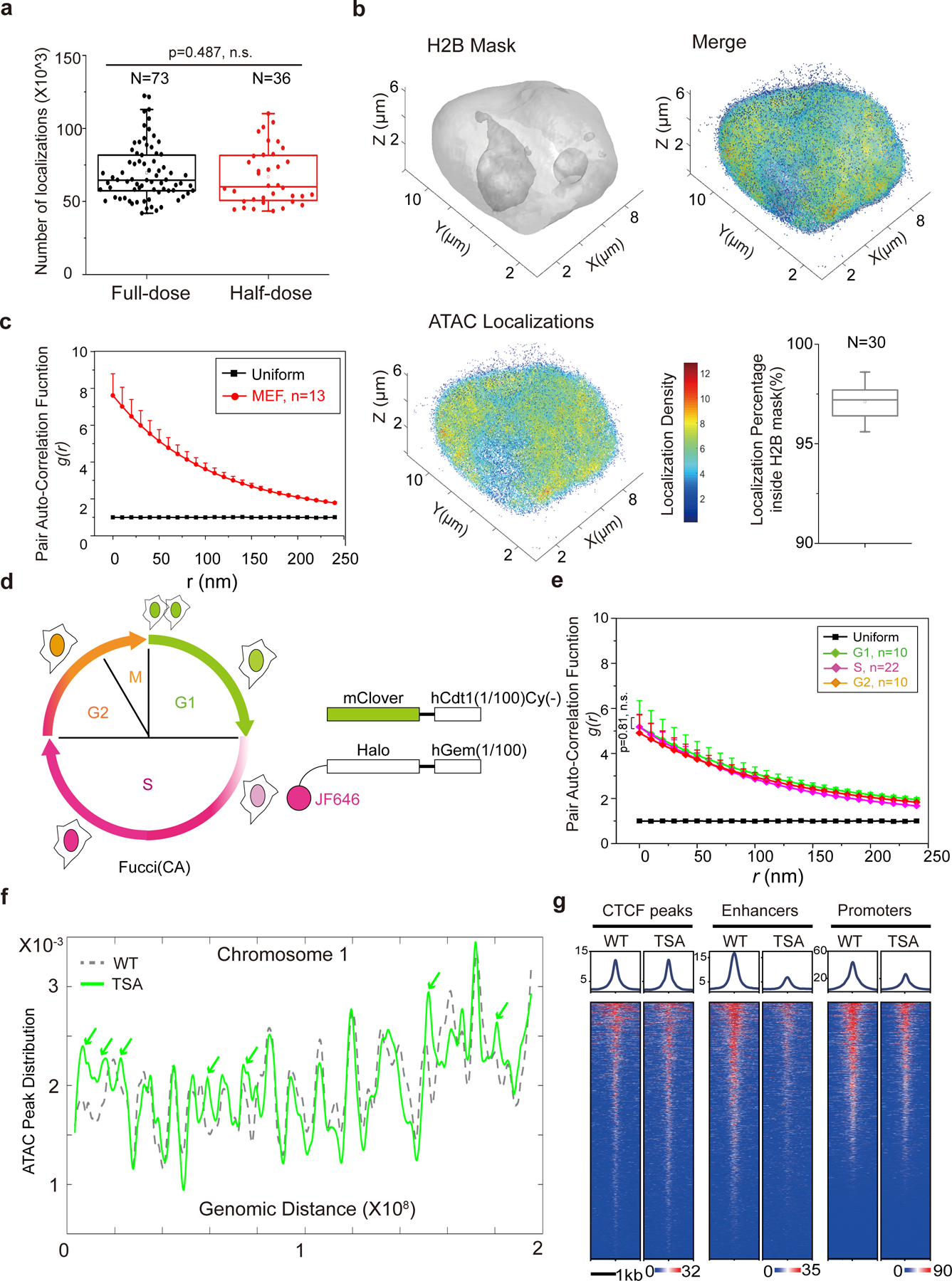
a, The box plot compares the number of 3D ATAC-PALM localizations in the full-dose (73 cells, ~100 nM Tn5 PA-JF₅₄₉) and half-dose (36 cells, ~50 nM) labeling conditions. The middle line represents median. The two-sided Student’s t-test was performed.

b, ATAC-PALM localizations (lower left) were separated as in-nucleus and out-nucleus fractions based on the H2B-GFP mask (upper left). The merged image was shown in the upper right panel. The color bar indicates the localization density calculated by using a canopy radius of 250 nm. Lower right panel shows the percentage of localizations falling into the H2B-GFP mask from 30 cells. The middle line represents median.

c, Pair auto-correlation function g(r) of ATAC-PALM localizations calculated for MEFs. The center curve represents the mean value and the error bars represent S.E.M.

d, Schematics for the FUCCI(CA) system in which the first 100 amino acids of hCdt1 lacking the Cy motif (1/100) Cy(−) is fused to mClover and the first 100 amino acids of hGeminin is fused to HaloTag stained by the JF₆₄₆ HaloTag ligand. G1 phase cells exhibit only green and S phase cells display only far red fluorescence, whereas dual color positive cells correspond to G2/M phase.

e, Pair auto-correlation function g(r) for ATAC-PALM localizations calculated across different cell cycle phases. The error bars represent S.E.M. The two-sided Mann-Whitney U test was performed.

f, ATAC-seq peak density distribution in the WT (grey line) and TSA treated (green line) cells for each of 500 bins across chromosome 1. Green arrowheads indicate new accessible chromatin induced by TSA treatment.

g, Heatmaps of ATAC-seq signal were plotted over CTCF binding sites (putative insulator sites), enhancers (defined by H3K27ac ChIP-seq) and promoter regions in the mouse genome with DMSO or TSA treatment (50μM, 6h).

Statistics source data are provided in Source Data Extended Figure 2.

Extended Data Figure 3 |. Two-color 3D PALM imaging of accessible chromatin and landmark proteins in the active chromatin.

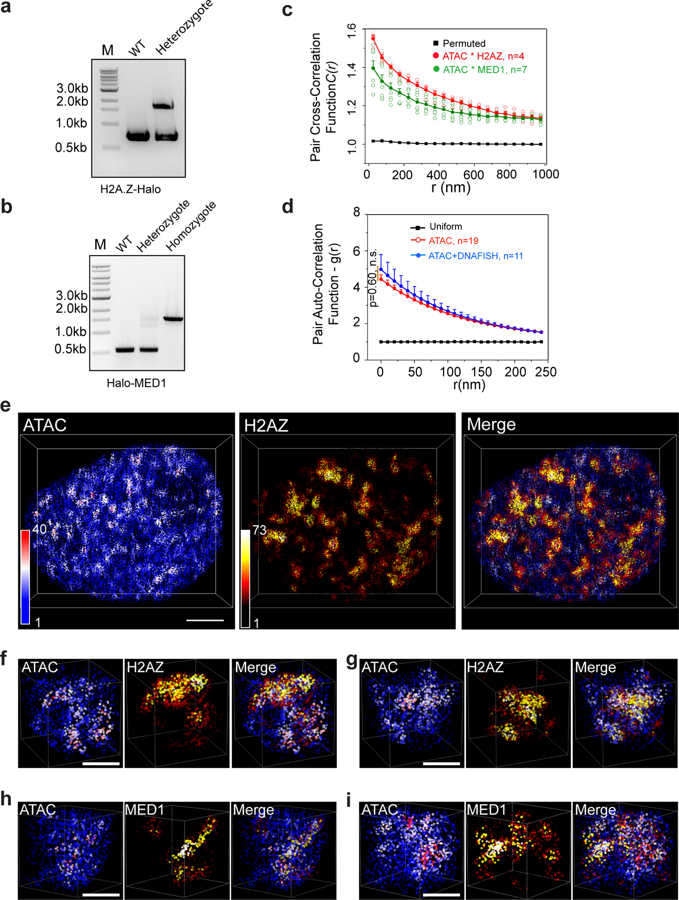
a and b, PCR genotyping validates the correct knock-in of HaloTag in frame with histone variant H2A.Z (a) or Mediator subunit MED1 (b) coding sequence in mESCs. We obtained heterozygous and homozygous HaloTag labeling to endogenous H2A.Z and MED1, respectively. All knock-in cells were validated by Sanger sequencing. Experiments were repeated two times.

c, 2D pair cross-correlation function C(r) calculated for accessible chromatin localizations and H2A.Z or MED1, in contrast to that of HP1 in Fig.2g. Circles represent mean values for cross-correlation function at a given radius (r). The error bars represent S.E.M.

d, Comparison of pair auto-correlation function g(r) calculated with ATAC labeling alone and ATAC labeling - DNA FISH condition. The error bars represent S.E.M. The two-sided Mann-Whitney U test was performed.

e, 3D illustration of colocalized accessible chromatin and HaloTag labeled H2A.Z protein localizations within a single nucleus. The color-coded localization density was calculated with a canopy radius of 250 nm. Scale bar: 2μm. The accessible chromatin was labelled with PA-JF₅₄₉, while H2A.Z-HaloTag molecules were labelled with PA-JF₆₄₆.

f and g, 3D illustration of colocalized accessible chromatin and HaloTag labeled H2A.Z protein localizations in representative sub-regions with volume of 2μm×2μm×2μm. Scale bar: 1μm.

h and i, 3D illustration of colocalized accessible chromatin and HaloTag-MED1 protein localizations in representative sub-regions with volume of 2μm×2μm×2μm. Scale bar: 1μm. Experiments were repeated 3 times and data were pooled together for analysis for (d)-(h).

Statistics source data are provided in Source Data Extended Figure 3.

Extended Data Figure 4 |. Efficient depletion of CTCF by the AID degron system.

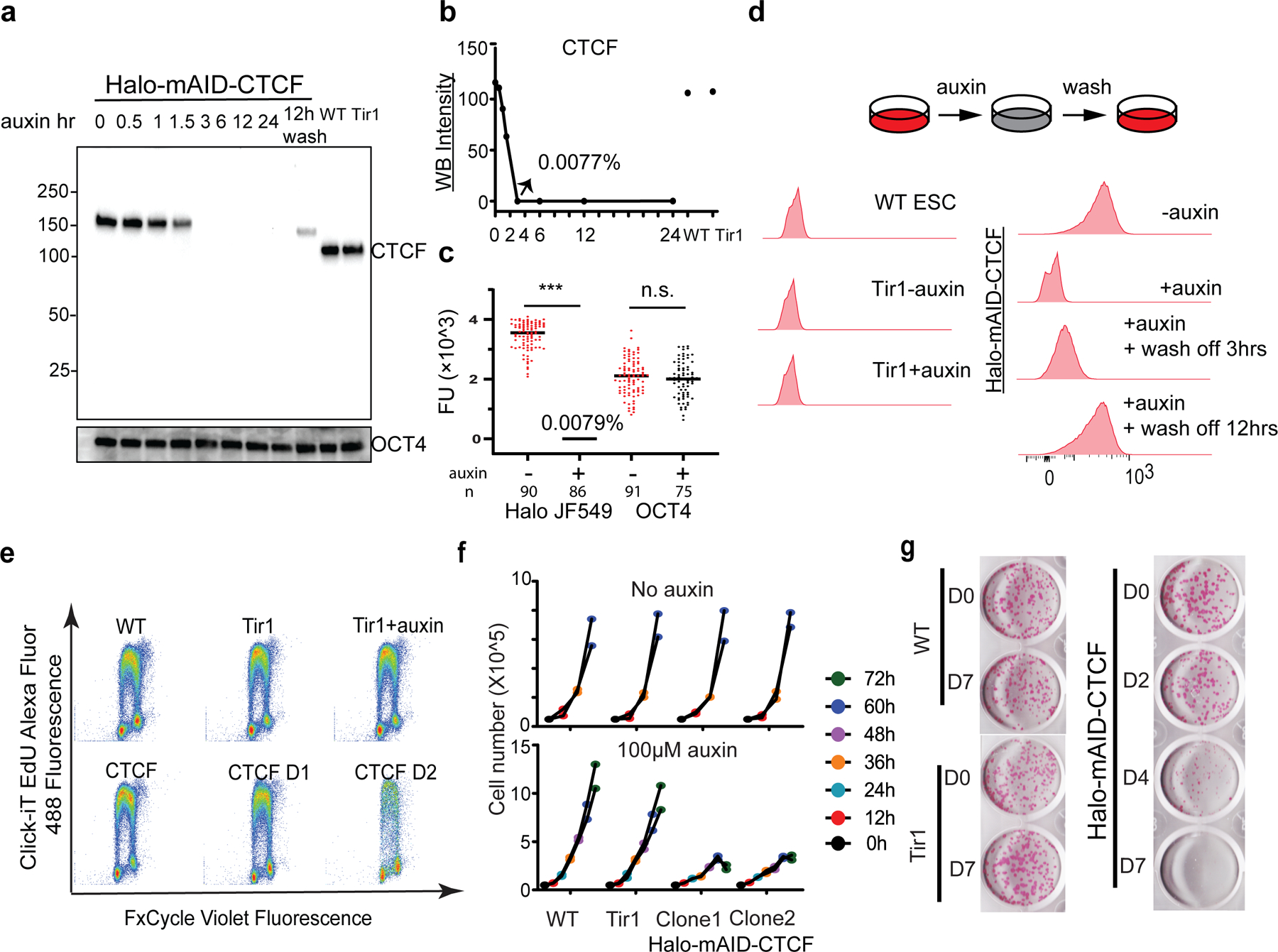
a, Western blotting (WB) analysis of endogenous HaloTag-mAID-CTCF at indicated time points after the auxin treatment and wash off recovery with OCT4 as the internal control.

b, Quantifying WB intensity as grey scale values for the corresponding WB bands in (a).

c, Single cell analysis of HaloTag-mAID-CTCF and OCT4 protein levels after auxin treatment. HaloTag-mAID-CTCF was stained with 100nM HaloTag ligand JF₅₄₉ and OCT4 was detected by immunofluorescence. FU stands for arbitrary fluorescent unit, with extra-cellular background subtracted. The middle line represents mean fluorescence value. Experiment was repeated two times for (a)-(c) with similar results. Two-sided Mann-Whitney U test was used for analysis with p value for Halo JF549 group < 0.0001 and for OCT4 group 0.3232

d, Flow cytometry analysis of CTCF levels before (-auxin), after (+auxin) auxin treatment and after auxin wash off. The parent Tir1 ES cells (Tir1 – Auxin; Tir1 + Auxin) were used as the negative control. ~50,000 gated live cells were recorded and analyzed for each condition. Experiments were repeated three times.

e, DNA synthesis analysis of HaloTag-mAID-CTCF ESCs by the Click-iT EdU labeling kit at the indicated time points (D, Days) after auxin treatment. Experiments were performed two times and representative images are shown.

f, Cell proliferation analysis of Wild type (WT), parental Tir1, and two clones of Halo-mAID-CTCF ESCs. Upper panel, without auxin treatment, different cell lines showed similar growth rates. Lower panel, acute CTCF depletion significantly slowed down cell proliferation after 36 hours (two-tailed Student’s t-test with p value < 0.05). Data from two technical replicates from two N-CTCF-mAID clones were shown.

g, Single cell colony formation assay by alkaline phosphatase staining for WT, parental Tir1, and Halo-mAID-CTCF ESCs at indicated time points after auxin treatment. Biological replicates n = 2.

Statistics source data are provided in Source Data Extended Figure 4.

Extended Data Figure 5 |. Enhanced clustering of ACDs upon CTCF depletion.

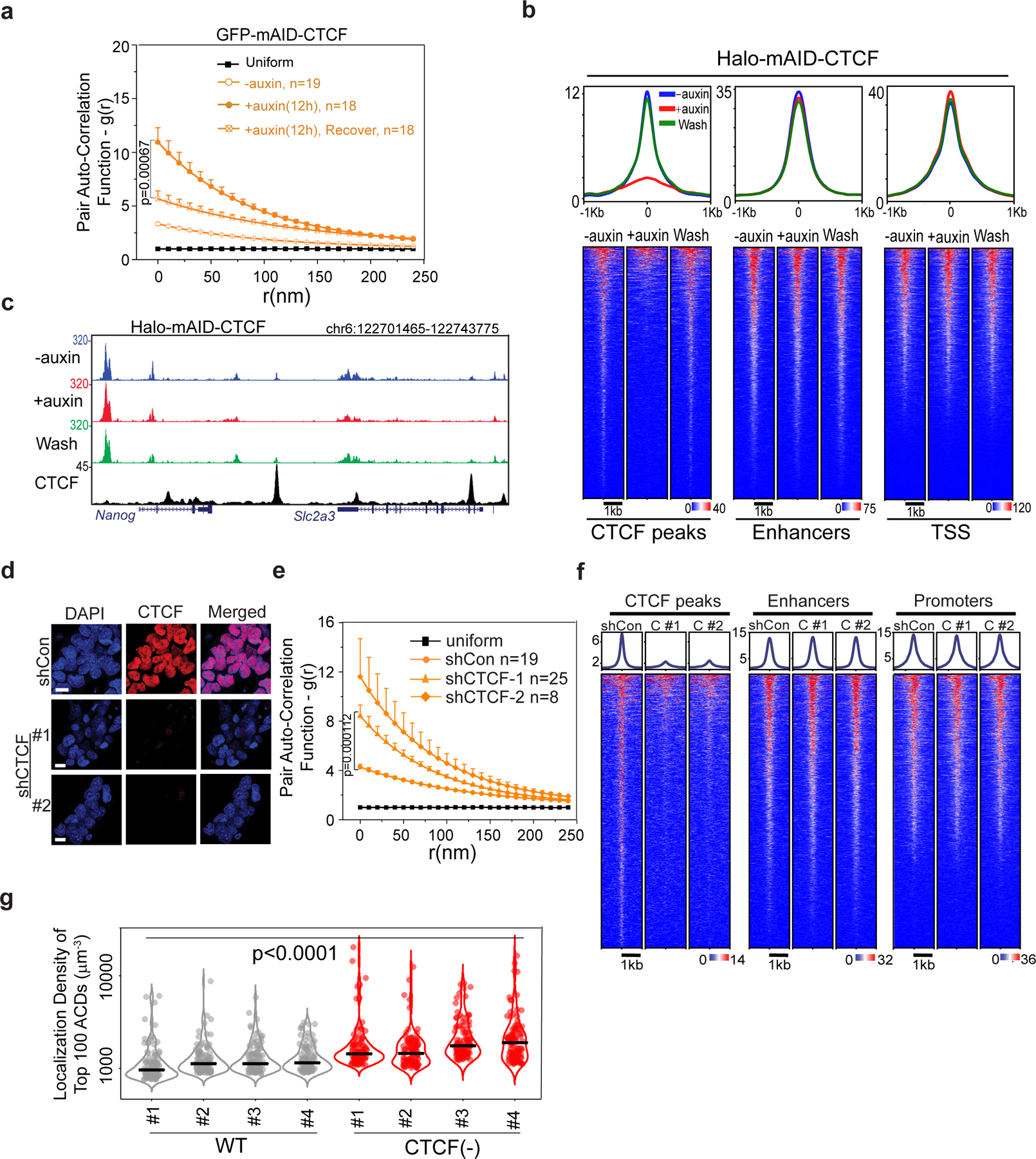
a, Pair auto-correlation function g(r) of ATAC-PALM localizations from GFP-mAID-CTCF ESCs under normal, auxin-treated and auxin wash-off (~24 hours) conditions. The error bars represent S.E.M. Two-sided Mann-Whitney U test was performed.

b, HaloTag-mAID-CTCF cells were processed for genome-wide ATAC-seq analysis under conditions including without auxin, auxin treatment and washout after auxin treatment. Three biological replicates were performed.

c, ATAC-seq enrichment at a representative genomic region under normal (-auxin), auxin-treated (+auxin) and recovery conditions for HaloTag-mAID-CTCF cells. CTCF ChIP-seq track is displayed below as a reference. Experiments were performed 3 times.

d, Bi-allelic CTCF-HaloTag knock-in cells were infected with either lentiviral particles containing the empty vector (shCon) or lentiviral vectors expressing two independent shRNAs against CTCF (#1 and #2). Cells were selected with Puromycin for two days and stained with 200nM JF₅₄₉ HaloTag ligand and DAPI before confocal imaging. Biological replicates n = 2.

e, Enhanced accessible chromatin clustering after shRNA mediated CTCF knockdown, which was monitored by staining cells with 200nM JF₆₄₆. The g(r) analysis of 3D ATAC-PALM localizations showed significant increased g(0) in CTCF knockdown cells, compared with control cells. The curve center represents the mean and the error bar represents S.E.M. The two-sided Mann-Whitney U test was performed.

f, CTCF knockdown cells were processed for genome-wide ATAC-seq analysis. CTCF knockdown by both shRNAs (C #1 and C #2) markedly reduced the chromatin accessibility at CTCF binding sites compared to shCon cells without significantly affecting that at enhancers and promoters.

g, Violin plot of localization density of top 100 rank ordered ACDs among 4 individual cells for each condition. The black bar indicates the median value. For statistical test, data from 4 individual cells for each condition were pooled together and two-sided Mann-Whitney U test was applied.

Statistics source data are provided in Source Data Extended Figure 5.

Extended Data Figure 6 |. Measuring structural changes of ATAC-rich and ATAC-poor segments upon CTCF depletion by Oligopaint DNA-FISH.

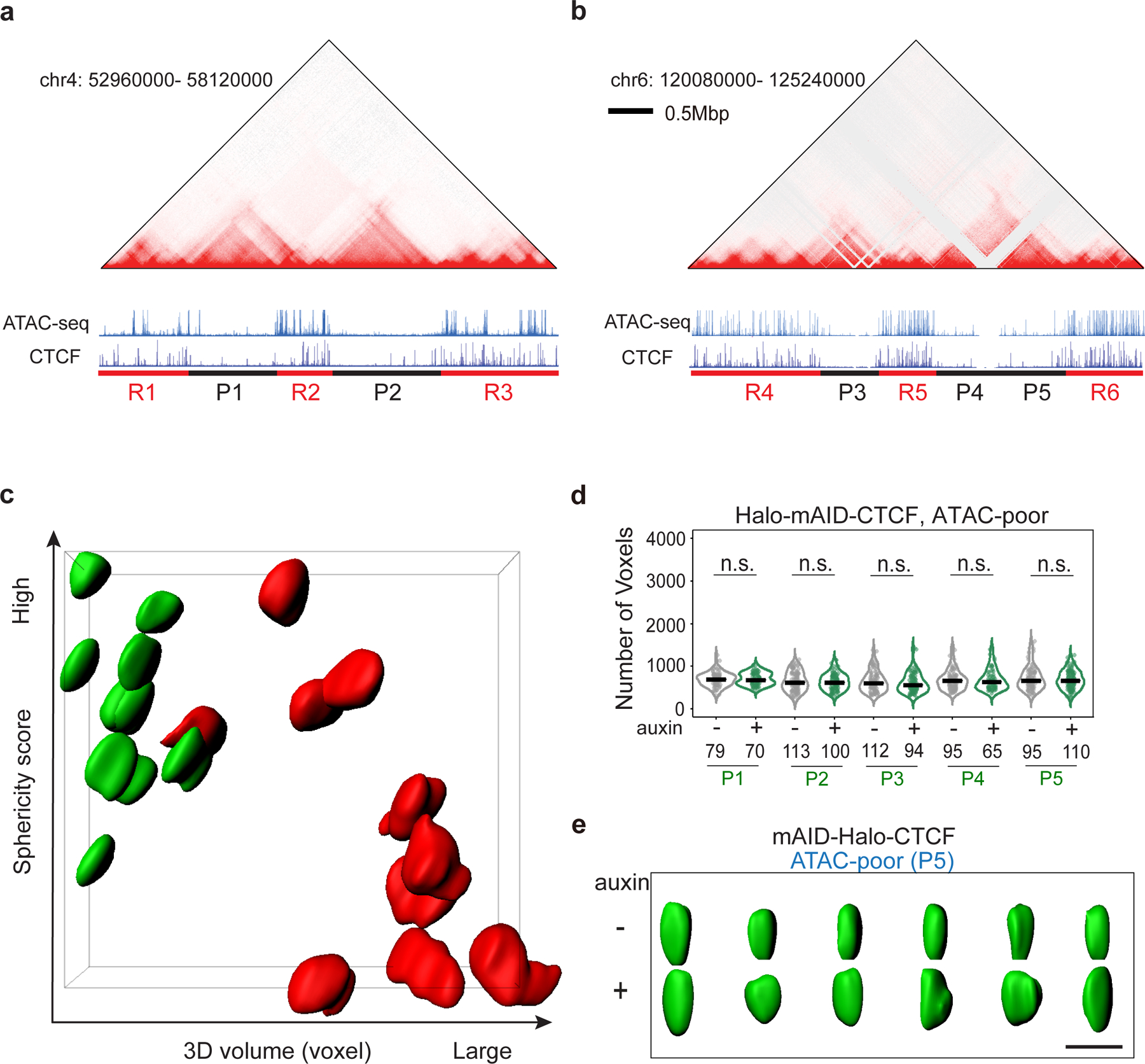
a-b, Alignment of Hi-C heatmap, ATAC-seq, CTCF ChIP-seq tracks for two chromosomal regions harboring pluripotency genes Klf4 (Chr4) and Nanog (Chr6). ATAC-rich (R1–6; red) and ATAC-poor (P1–5; black) segments are underlined. The sizes of each domain are R1(633kb),P1(1133kb), R2(643kb), P2(1100kb), R3(1120kb), R4(1250kb), P3(740kb), R5(640kb), P4(690kb), P5(690kb), R6(990kb). See details on the domain coordinates in the Methods.

c, Two-dimensional sphericity score and 3D volume (by voxels) plot of all the ATAC-rich and ATAC-poor segments (iso-surfaces) in Supplementary Video 6 marked by 3D Oligopaint DNA-FISH probes.

d, Violin plot of 3D volumes (the number of voxels) of five ATAC-poor segments (P1–P5) before and after CTCF depletion. Throughout the volume measurements in this study, each voxel size is x=48.9 nm, y=48.9 nm, z=199 nm. The number (n) of alleles analyzed is indicated at the bottom. The black bar indicates the median value for each data set and two-sided Mann-Whitney U test was applied for statistical test. P-values for P1–P5 are: p1=0.585, p2=0.932, p3=0.226, p4=0.849, p5=0.853.

e, Representative iso-surfaces of an ATAC-poor segment (P5, green) before (−) and after (+) CTCF depletion (12 hours). Scale bar, 1 μm. Biological replicates n=3.

Statistics source data are provided in Source Data Extended Figure 6.

Extended Data Figure 7 |. CTCF depletion significantly reduced the number of loops and the degree of TAD domain insulation by high-resolution Micro-C analysis.

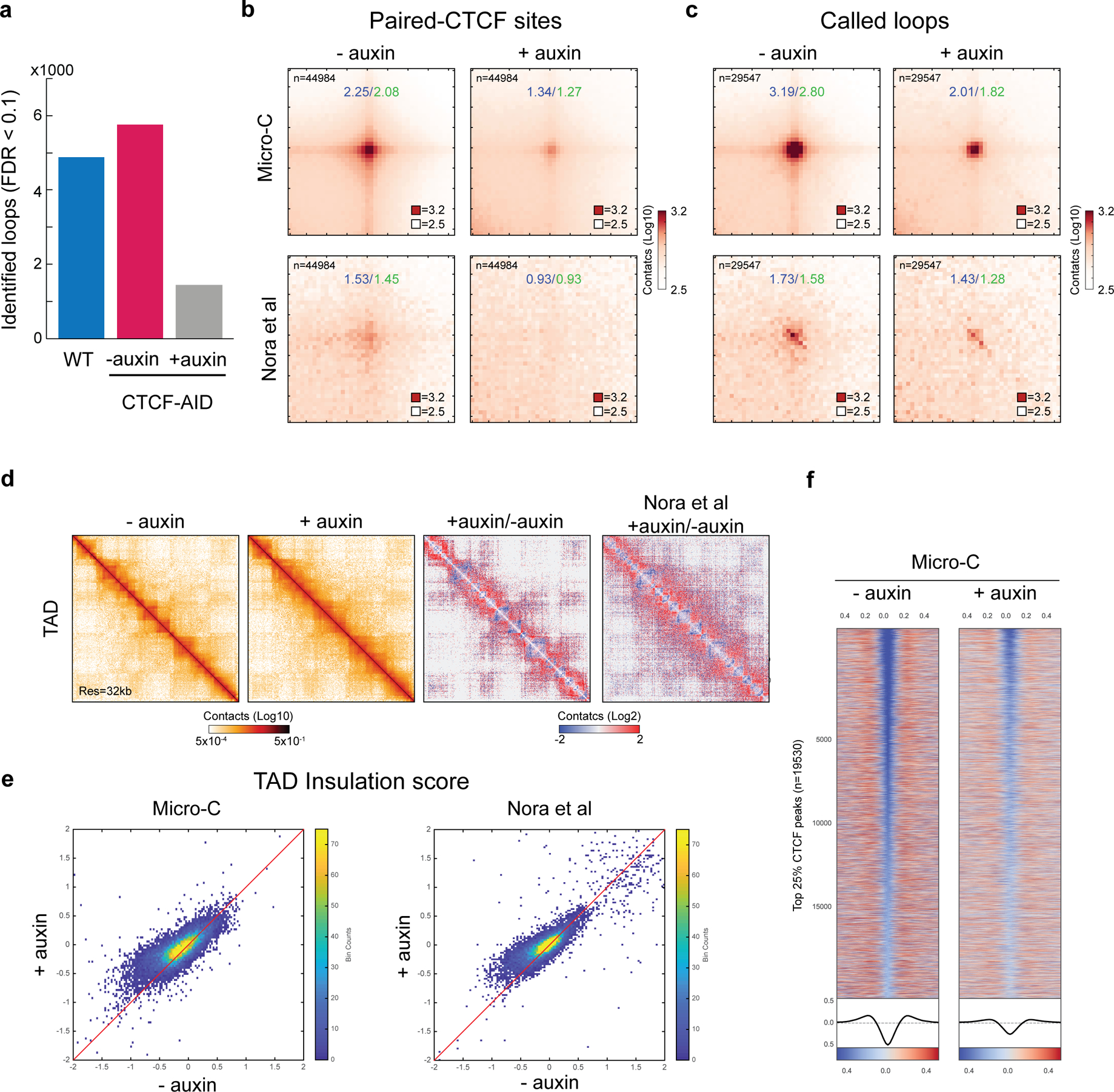
a, Number of loops in WT-mESC, CTCF-AID mESC -auxin, and +auxin conditions. We identified a similar number of loops in WT-mESC (n=4887) and CTCF-AID mESC -auxin (n=5764), while only 1442 loops were identified after CTCF depletion under identical loop calling criteria. We performed two biological replicates and the data was pooled for analysis.

b-c, Aggregate peak analysis on paired-CTCF sites or called loops from Micro-C and Hi-C ¹data. Loops were greatly disrupted in Micro-C data after CTCF depletion, which showed a 1.67-fold decrease at CTCF sites or 1.59-fold decrease at called loop loci, respectively. We obtain much fewer loops from previous Hi-C data likely due to the lower resolution¹.

d, Snapshots of Micro-C contact maps on chr8:80M-95M at 32-kb resolution. Contact maps showed more inter-TAD contacts (loss of insulation) and modestly higher inter-compartment domain contacts after CTCF depletion. Hi-C data also showed a similar result but with a slightly different plaid-like pattern.

e, Heatmap of insulation strength at CTCF-binding sites. Insulation strength was over 2-fold decrease at the top 25% of CTCF binding sites after CTCF depletion.

f, Scatter plots of insulation strength at the called boundaries. Micro-C and Hi-C both showed consistent insulation loss (higher insulation score) after CTCF depletion.

Extended Data Figure 8 |. CTCF depletion significantly increased the contact probability in A compartment by high-resolution Micro-C analysis.

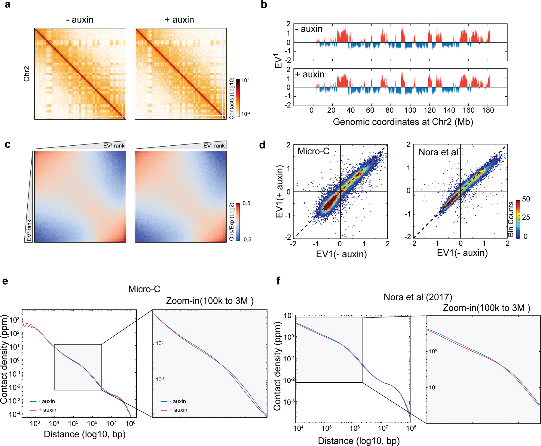
a, Snapshots of Micro-C contact maps on the entire Chr2, showing the plaid-like compartments before and after auxin-mediated CTCF depletion (6 hours).

b, Compartment analysis by principle component analysis (PCA). The plots showed the eigenvector of the first PCA. Positive value is compartment A, and negative value is compartment B. There is no noticeable change in the large-scale compartment organization after CTCF depletion.

c, Genome-wide analysis of the compartment strength. The saddle plot showed the contact probability between compartments and showed B-B on the top-left corner and A-A on the bottom-right corner. There is no significant compartment change after CTCF depletion.

d, Comparison of compartment change in Micro-C and Hi-C. No dramatic change was found, albeit Micro-C appears to capture more changes in compartment strength than Hi-C after CTCF depletion.

e-f, Genome-wide contact probability decaying curve by Micro-C (e) and Hi-C (f). See also Fig.3h. Data from two biological replicates was pooled for analysis.

References:

- 1.Dekker J et al. The 4D nucleome project. Nature 549, 219–226 (2017). [DOI] [PMC free article] [PubMed] [Google Scholar]
- 2.Dekker J et al. Capturing chromosome conformation. Science 295, 1306–11 (2002). [DOI] [PubMed] [Google Scholar]
- 3.De Wit E& De Laat W A decade of 3C technologies: insights into nuclear organization. Genes Dev. 26, 11–24 (2012). [DOI] [PMC free article] [PubMed] [Google Scholar]
- 4.Dekker J & Mirny L The 3D Genome as Moderator of Chromosomal Communication. Cell 164, 1110–1121 (2016). [DOI] [PMC free article] [PubMed] [Google Scholar]
- 5.Dekker J, Marti-Renom MA & Mirny LA Exploring the three-dimensional organization of genomes: Interpreting chromatin interaction data. Nature Reviews Genetics 14, 390–403 (2013). [DOI] [PMC free article] [PubMed] [Google Scholar]
- 6.Finn E et al. Extensive Heterogeneity and Intrinsic Variation in Spatial Genome Organization. Cell 176, 1502–1515 (2019). [DOI] [PMC free article] [PubMed] [Google Scholar]
- 7.Levine M, Cattoglio C & Tjian R Looping back to leap forward: Transcription enters a new era. Cell 157, 13–25 (2014). [DOI] [PMC free article] [PubMed] [Google Scholar]
- 8.Wu C The 5’ ends of drosophila heat shock genes in chromatin are hypersensitive to DNase I. Nature 286, 854–860 (1980). [DOI] [PubMed] [Google Scholar]
- 9.Boyle AP et al. High-Resolution Mapping and Characterization of Open Chromatin across the Genome. Cell (2008). doi: 10.1016/j.cell.2007.12.014 [DOI] [PMC free article] [PubMed] [Google Scholar]
- 10.Buenrostro JD, Giresi PG, Zaba LC, Chang HY & Greenleaf WJ Transposition of native chromatin for fast and sensitive epigenomic profiling of open chromatin, DNA-binding proteins and nucleosome position. Nat. Methods 10, 1213–8 (2013). [DOI] [PMC free article] [PubMed] [Google Scholar]
- 11.Buenrostro JD et al. Single-cell chromatin accessibility reveals principles of regulatory variation. Nature 523, 486–490 (2015). [DOI] [PMC free article] [PubMed] [Google Scholar]
- 12.Chen X et al. ATAC-see reveals the accessible genome by transposase-mediated imaging and sequencing. Nat. Methods 13, 1013–1020 (2016). [DOI] [PMC free article] [PubMed] [Google Scholar]
- 13.Grimm JB et al. Bright photoactivatable fluorophores for single-molecule imaging. Nature Methods 13, 985–988 (2016). [DOI] [PubMed] [Google Scholar]
- 14.Betzig E et al. Imaging intracellular fluorescent proteins at nanometer resolution. Science 313, 1642–5 (2006). [DOI] [PubMed] [Google Scholar]
- 15.Chen BC et al. Lattice light-sheet microscopy: Imaging molecules to embryos at high spatiotemporal resolution. Science (80-. ). 346, 1257998 (2014). [DOI] [PMC free article] [PubMed] [Google Scholar]
- 16.Legant WR et al. High-density three-dimensional localization microscopy across large volumes. Nat. Methods 13, 359–365 (2016). [DOI] [PMC free article] [PubMed] [Google Scholar]
- 17.Huang B, Wang W, Bates M & Zhuang X Three-dimensional super-resolution imaging by stochastic optical reconstruction microscopy. Science (80-. ). 319, 810–813 (2008). [DOI] [PMC free article] [PubMed] [Google Scholar]
- 18.Beliveau BJ et al. Versatile design and synthesis platform for visualizing genomes with Oligopaint FISH probes. Proc. Natl. Acad. Sci 109, 21301–21306 (2012). [DOI] [PMC free article] [PubMed] [Google Scholar]
- 19.Beliveau BJ et al. Single-molecule super-resolution imaging of chromosomes and in situ haplotype visualization using Oligopaint FISH probes. Nat. Commun 7147 (2015). doi: 10.1038/ncomms8147 [DOI] [PMC free article] [PubMed] [Google Scholar]
- 20.Boettiger AN et al. Super-resolution imaging reveals distinct chromatin folding for different epigenetic states. Nature 529, 418–422 (2016). [DOI] [PMC free article] [PubMed] [Google Scholar]
- 21.Wang S et al. Spatial organization of chromatin domains and compartments in single chromosomes. Science (80-. ). 353, 598–602 (2016). [DOI] [PMC free article] [PubMed] [Google Scholar]
- 22.Peebles PJE Statistical Analysis of Catalogs of Extragalactic Objects. I. Theory. Astrophys. J 185, 413 (1973). [Google Scholar]
- 23.Sengupta P et al. Probing protein heterogeneity in the plasma membrane using PALM and pair correlation analysis. Nat. Methods 8, 969–975 (2011). [DOI] [PMC free article] [PubMed] [Google Scholar]
- 24.Ester M, Kriegel HP, Sander J, & Xu X A Density-Based Algorithm for Discovering Clusters in Large Spatial Databases with Noise. Kdd 96, 226–231 (1996). [Google Scholar]
- 25.Sakaue-Sawano A et al. Genetically Encoded Tools for Optical Dissection of the Mammalian Cell Cycle. Mol. Cell 68, 626–640.e5 (2017). [DOI] [PubMed] [Google Scholar]
- 26.Kieffer-Kwon KR et al. Myc Regulates Chromatin Decompaction and Nuclear Architecture during B Cell Activation. Mol. Cell 67, 566–578.e10 (2017). [DOI] [PMC free article] [PubMed] [Google Scholar]
- 27.Bintu B et al. Super-resolution chromatin tracing reveals domains and cooperative interactions in single cells. Science (80-. ). 362, eaau1783 (2018). [DOI] [PMC free article] [PubMed] [Google Scholar]
- 28.Finn EH et al. Extensive Heterogeneity and Intrinsic Variation in Spatial Genome Organization. Cell (2019). doi: 10.1016/j.cell.2019.01.020 [DOI] [PMC free article] [PubMed] [Google Scholar]
- 29.Sabari BR et al. Coactivator condensation at super-enhancers links phase separation and gene control. Science (80-. ). 361, 387–392 (2018). [DOI] [PMC free article] [PubMed] [Google Scholar]
- 30.Jin C et al. H3.3/H2A.Z double variant-containing nucleosomes mark ‘nucleosome-free regions’ of active promoters and other regulatory regions. Nat. Genet (2009). doi: 10.1038/ng.409 [DOI] [PMC free article] [PubMed] [Google Scholar]
- 31.Nora EP et al. Targeted Degradation of CTCF Decouples Local Insulation of Chromosome Domains from Genomic Compartmentalization. Cell 169, 930–944.e22 (2017). [DOI] [PMC free article] [PubMed] [Google Scholar]
- 32.Nishimura K, Fukagawa T, Takisawa H, Kakimoto T & Kanemaki M An auxin-based degron system for the rapid depletion of proteins in nonplant cells. Nat. Methods 6, 917–922 (2009). [DOI] [PubMed] [Google Scholar]
- 33.Wutz G et al. Topologically associating domains and chromatin loops depend on cohesin and are regulated by CTCF, WAPL, and PDS5 proteins. EMBO J. e201798004 (2017). doi: 10.15252/embj.201798004 [DOI] [PMC free article] [PubMed] [Google Scholar]
- 34.Hsieh THS et al. Mapping Nucleosome Resolution Chromosome Folding in Yeast by Micro-C. Cell (2015). doi: 10.1016/j.cell.2015.05.048 [DOI] [PMC free article] [PubMed] [Google Scholar]
- 35.Hsieh T-HS et al. Resolving the 3D landscape of transcription-linked mammalian chromatin folding. bioRxiv (2019). doi: 10.1101/638775 [DOI] [PMC free article] [PubMed] [Google Scholar]
- 36.Fudenberg G et al. Formation of Chromosomal Domains by Loop Extrusion. Cell Rep. 15, 2038–2049 (2016). [DOI] [PMC free article] [PubMed] [Google Scholar]
- 37.Sanborn AL et al. Chromatin extrusion explains key features of loop and domain formation in wild-type and engineered genomes. Proc. Natl. Acad. Sci 112, E6456–E6465 (2015). [DOI] [PMC free article] [PubMed] [Google Scholar]
- 38.Alipour E & Marko JF Self-organization of domain structures by DNA-loop-extruding enzymes. Nucleic Acids Res. 40, 11202–11212 (2012). [DOI] [PMC free article] [PubMed] [Google Scholar]
- 39.Fudenberg G, Abdennur N, Imakaev M, Goloborodko A & Mirny LA Emerging Evidence of Chromosome Folding by Loop Extrusion. Cold Spring Harb. Symp. Quant. Biol (2017). doi: 10.1101/sqb.2017.82.034710 [DOI] [PMC free article] [PubMed] [Google Scholar]
- 40.Li G et al. Extensive promoter-centered chromatin interactions provide a topological basis for transcription regulation. Cell 148, 84–98 (2012). [DOI] [PMC free article] [PubMed] [Google Scholar]
- 41.Xie L et al. A dynamic interplay of enhancer elements regulates Klf4 expression in naïve pluripotency. Genes Dev. 31, 1795–1808 (2017). [DOI] [PMC free article] [PubMed] [Google Scholar]
- 42.Chen KH, Boettiger AN, Moffitt JR, Wang S & Zhuang X Spatially resolved, highly multiplexed RNA profiling in single cells. Science (80-. ). 348, 356–372 (2015). [DOI] [PMC free article] [PubMed] [Google Scholar]
- 43.Shah S et al. Dynamics and Spatial Genomics of the Nascent Transcriptome by Intron seqFISH. Cell 174, 363–376.e16 (2018). [DOI] [PMC free article] [PubMed] [Google Scholar]
- 44.Corces MR et al. The chromatin accessibility landscape of primary human cancers. Science (80-. ). (2018). doi: 10.1126/science.aav1898 [DOI] [PMC free article] [PubMed] [Google Scholar]
- 45.Picelli S et al. Tn5 transposase and tagmentation procedures for massively scaled sequencing projects. Genome Res. 24, 2033–2040 (2014). [DOI] [PMC free article] [PubMed] [Google Scholar]
- 46.Liu Z et al. 3D imaging of Sox2 enhancer clusters in embryonic stem cells. Elife 3, 1–29 (2014). [DOI] [PMC free article] [PubMed] [Google Scholar]
- 47.Kiskowski MA, Hancock JF & Kenworthy AK On the use of Ripley’s K-function and its derivatives to analyze domain size. Biophys. J 97, 1095–1103 (2009). [DOI] [PMC free article] [PubMed] [Google Scholar]
- 48.Veatch SL et al. Correlation functions quantify super-resolution images and estimate apparent clustering due to over-counting. PLoS One (2012). doi: 10.1371/journal.pone.0031457 [DOI] [PMC free article] [PubMed] [Google Scholar]
Associated Data
This section collects any data citations, data availability statements, or supplementary materials included in this article.