Coupling the Macroscale to the Microscale in a Spatiotemporal Context to Examine Effects of Spatial Diffusion on Disease Transmission

Abstract

There are many challenges to coupling the macroscale to the microscale in temporal or spatial contexts. In order to examine effects of an individual movement and spatial control measures on a disease outbreak, we developed a multiscale model and extended the semi-stochastic simulation method by linking individual movements to pathogen’s diffusion, linking the slow dynamics for disease transmission at the population level to the fast dynamics for pathogen shedding/excretion at the individual level. Numerical simulations indicate that during a disease outbreak individuals with the same infection status show the property of clustering and, in particular, individuals’ rapid movements lead to an increase in the average reproduction number $R_0$, the final size and the peak value of the outbreak. It is interesting that a high level of aggregation the individuals’ movement results in low new infections and a small final size of the infected population. Further, we obtained that either high diffusion rate of the pathogen or frequent environmental clearance lead to a decline in the total number of infected individuals, indicating the need for control measures such as improving air circulation or environmental hygiene. We found that the level of spatial heterogeneity when implementing control greatly affects the control efficacy, and in particular, an uniform isolation strategy leads to low a final size and small peak, compared with local measures, indicating that a large-scale isolation strategy with frequent clearance of the environment is beneficial for disease control.

Introduction

The transmission of infectious diseases exhibits spatiotemporal multiple-scale properties, including transmission dynamics at the population level, with viral replication and interaction with targeted cells at the individual level. Moreover, between-host disease transmission is generally dependent on the within-host viral loads, and vice versa. Also, different enteroviral serotypes greatly influence the between-host transmission. A number of mathematical models of infectious diseases have been studied extensively by employing single-scale-based models at the immunological or epidemiological scales (Anderson and May 1991; Nowak and May 2000; Diekmnann and Heesterbeek 2000). The immunological models focus on the within-host immune viral dynamics at the individual level, while the epidemiological models focus on the between-host transmission dynamics at the population level. Availability of big data at various levels and emergence of unanswered questions enable novel methods of mathematical models to connect within-host immune viral dynamics with the between-host epidemiological transmission of infectious diseases.

A multiscale immuno-epidemiological modeling approach has become an emerging method to study the synergistic dynamics of pathogens/viruses at the individual and population levels (Gog et al. 2015; Shen et al. 2015; Sun et al. 2016; Hosseini and Gabhann 2012; Dorratoltaj et al. 2017; Bauer et al. 2009). Furthermore, the mechanisms and processes (transmission, replication, pathogen shedding, infection) for infectious disease systems can be modeled for each hierarchical level. These can then be coupled via bridges between the microscale and the macroscale, leading to similar categories of multiscale models which include individual-based multiscale models (IMSMs), nested multiscale models (NMSMs), embedded multiscale models (EMSMs) and hybrid multiscale models (HMSMs) (Garira 2017, 2018; Feng et al. 2012; Murillo et al. 2013; Gandolfi et al. 2014; Yu and Bagheri 2016). Agent(individual)-based models (ABMs or IBMs) are particularly well suited to characterize biological phenomena in a multiscale, multiclass manner. In particular, they can simulate ensembles of individual hosts in time and space, represent detailed information on epidemic states and contribute to our understanding of disease pathology and epidemiology (Sun et al. 2016; Bauer et al. 2009).

In the environmental transmission of some infectious diseases, pathogen shedding/excretion and pathogen transmission are the two main processes by which the fundamental mechanisms at the microscale and the macroscale may be coupled and influence each other (Feng et al. 2012, 2013). The microscale submodel and the macroscale submodel may be described by either the same or different formalisms (mathematical representations). Numerical computation becomes quite hard for various formalisms, with examples of such paired formalisms being deterministic/stochastic, discrete time/continuous time, mechanistic/phenomenological (Sun et al. 2016; Wang et al. 2012, 2015; Wang and Tang 2017). In particular, it is challenging to simultaneously simulate random moving events, epidemic processes (transmission, recovery and etc) of individuals as well as the pathogen’s shedding/excretion, transmission and continuous diffusion.

The main purpose of this study is to develop the computational methods to deal with two spatial scales (randomly moving individuals and continuous diffusion of bacteria) and temporal scales (slow dynamics of disease transmission at the population scale and fast dynamics for pathogen shedding/excretion at the individual level), in order to examine how the spatial movements of individuals and/or pathogens affect the infectious disease and, in particular, the cumulative number in the infected population and the average reproduction number. It is a systematic analysis of the effects of individual random walks in space, virus particles’ diffusion and a threshold control policy on the transmission of infectious diseases.

Individual-Based Stochastic Simulation Models (IBMs)

To describe the coupling of random movement of individuals in space, an epidemic process and the release and diffusion of pathogens, we initially present how to simulate the individuals’ epidemic process and movement based on individual-based stochastic simulations. Then we link this stochastic simulation to the pathogen dynamics with a partial differential equation. Finally, we simulate some interventions to examine effects of control strategies on outbreaks. In order to show all of the possible processes clearly, we use the classic deterministic SIR-type epidemic model with both direct and indirect transmission of free-living pathogens (Anderson and May 1991; Diekmnann and Heesterbeek 2000). Note that when modeling indirect transmission, the grow of pathogen is mainly assumed to be dependent either only on the shed of the infected individuals or on both the shedding and its’ growth due to self-growing in reservoir (Codeco 2001; Joh et al. 2009; Kong et al. 2014; Tien and Earn 2010; Rohani et al. 2009; Mukandavire et al. 2011; Luo et al. 2017). Here we take the MRSA (Methicillin-resistant Staphylococcus aureus) and MRAB (multidrug-resistant Acinetobacter baumannii) induced infection in the hospital as examples to consider (Wang et al. 2012, 2015; Wang and Tang 2017). Consequently, we initially assume the pathogens grow only depending on the infected individuals’ shedding and leave other case for discussion. The model equations are:

$$\begin{array}{c}\hfill \left\{\begin{array}{ccc}\hfill \frac{\mathrm{d}S(t)}{\mathrm{d}t}& =& -\beta SI-\nu SW\hfill \\ \hfill \frac{\mathrm{d}I(t)}{\mathrm{d}t}& =& \beta SI+\nu SW-\gamma I\hfill \\ \hfill \frac{\mathrm{d}R(t)}{\mathrm{d}t}& =& \gamma I\hfill \\ \hfill \frac{\mathrm{d}W(t)}{\mathrm{d}t}& =& \eta I-(\mu +\nu N)W(t)\hfill \end{array}\right)\end{array}$$ 1

where S, I and R denote the number of susceptible, infected and recovered individuals, W(t) is the pathogen concentration in the environment at time t. The total population is constant N ($N=S+I+R$). Parameters $\beta$ and $\nu$ represent the direct and indirect transmission rates, respectively, and $\gamma$ denotes the recovery rate. $\eta$ denotes the pathogen shedding rate of infected individuals and $\mu$ denotes the rate of clearance of the pathogen from the environment.

The crucial question is how to deal with both the spatial and temporal scales (individuals’ random and relatively slow movements and the pathogen’s fast, wide-ranging diffusion) when we design the algorithms for the SIRW model (1). To do this, a semi-stochastic simulation method was employed, i.e., the variation amongst individuals (susceptible, infected and recovered individuals) are treated stochastically, while the dynamics of the bacterial changes are treated deterministically and follow the reaction–diffusion equation. Hence, stochastic simulation algorithms are used for the individuals’ dynamics and numerical method for the deterministic PDE equation is then applied to the variation amongst the free-living pathogens. Meanwhile, alternating direction implicit (ADI) time and space discretization schemes for model (1) will be employed (Peaceman and Rachford 1995).

IBMs Among Hosts: Epidemic Process and Random Moving

Epidemic process We formulate a general stochastic individual-based model by event-driven simulations, develop the numerical algorithm to simulate the spatially random walk and the pathogen’s diffusion. The event-driven approach using the direct Gillespie algorithm (Gillespie 1976, 1977; Keeling and Rohani 2008) can easily be adapted, and we get the stochastic simulation model with the following probabilities:

$(S,I)\to (S-1,I+1)$ with a probability of $\beta SI$,

$(I,R)\to (I-1,R+1)$ with a probability of $\gamma I$.

For spatial transmission events, we assume that an infected individual can only infect susceptibles within a certain radius rather than throughout the whole region. Spatial transmission is captured using a technique similar to the integro-differential equation model, then the transmission term (force of infection) to a susceptible individual i is given by:

$$\begin{array}{c}\hfill {\lambda }_i=\beta \sum _{j\in I}^{N_I}{K}_T(D_{\mathit{ij}}),\end{array}$$

where $D_{\mathit{ij}}$ is the distance between the susceptible individual i and an infectious individual j, and $K_T$ is the transmission kernel that measures how transmission decreases with distance $K_T(D_{\mathit{ij}})=D_{\mathit{ij}}^{-\alpha /2}$. Recovery of an infectious individual is independent of its position in space, hence the recovery rate of infectious individual j is constant $\gamma$.

Random moving To describe movement of individuals, we let individuals randomly and spontaneously move from their current location to a new location according to a local movement kernel. Meanwhile, to represent the aggregation effect among individuals, we assume that the velocity/direction of an individual’s movement is dependent on both his/her own original velocity/direction and the populations’ velocity/direction. Assume that the individuals were represented by points moving continuously (off-lattice) on the plane. Consider total population ($N=S+I+R$) at position $x(t)=(x_1(t),\dots ,x_N(t))$ moving with dimensionless velocities $v(t)=(v_1(t),\dots ,v_N(t))$ and direction angles $\theta (t)=({\theta }_1(t),\dots ,{\theta }_N(t))$. We can then write the movement dynamics as a system of difference Equations (DEs) as follows:

$$\begin{array}{c}\hfill \left\{\begin{array}{ccc}{x}_i(t+1)\hfill & =\hfill & x_i(t)+v_i(t+1),\hfill \\ v_i(t+1)\hfill & =\hfill & \sigma v_i(t)+(1-\sigma )v_{i0}\left(\begin{array}{cc}& cos({\theta }_i(t+1))\hfill \\ \hfill & sin({\theta }_i(t+1))\hfill \end{array}\right)\hfill \\ {\theta }_i(t+1)\hfill & =\hfill & {〈{\theta }_i,(t)〉}_r+\mathrm{\Delta }{\theta }_i.\hfill \end{array}\right)\end{array}$$ 2

where the velocity of an individual $v_i(t+1)$ is dependent on the initial velocity $v_{i0}$ and a direction given by the angle ${\theta }_i(t+1)$. Here ${〈{\theta }_i,(t)〉}_r$ denotes the average direction of the velocities of individuals (including individual i) being within a circle of radius r surrounding a given individual, the average direction was given by the angle

$$\begin{array}{c}\hfill \text{arctan}\left[\frac{sin{〈{\theta }_i,(t)〉}_r}{cos{〈{\theta }_i,(t)〉}_r}\right].\end{array}$$

$\mathrm{\Delta }{\theta }_i$ is a random number chosen with a uniform probability from the given interval. Note that here the angle of an individual’s movement at the next moment depends on two factors: the average moving angle of the population within a radius of clustering and random disturbance received by the current individual. Thus, the random perturbation may be strong enough such that an individual may move away from group movements and move independently. Similarly, the velocity of an individual’s movement at the next moment depends on its own movement speed and population movement speed with a weighted parameter $\sigma$. Thus, if $\sigma$ is relatively large, then an individual is more likely to move along its own way, while if $\sigma$ is relatively small, then the individual could be more significantly affected by group movement. Thus, the parameter $\sigma$ could describe the level of conformity (or bandwagon effect). The algorithm for the epidemic process and random movement is listed in “Appendix A1”.

IBMs Among Hosts and Pathogens: Epidemic Process and Hosts’ Movement/Pathogens’ Diffusion

To further consider diffusion of a free-living pathogen based on the individual-based simulation model, we assume that the infected individual can shed pathogens, and that pathogens can be taken to different places either by the movement of infected individuals or by movements in the air. Note that the susceptible individuals can be infected either by the infected individuals or by free-living pathogens (as shown in Fig. 1). There is a strong empirical evidence that humans have immunological thresholds for infections by waterborne diseases (Joh et al. 2009; Kong et al. 2014; Luo et al. 2017), it is thus interesting to incorporate an immunological threshold for infections when considering indirect transmission via free-living pathogen. We then assume that the pathogen can infect the susceptible individuals only when its concentration reaches a certain threshold value. That is, there is a positive threshold value $W_{\mathrm{c}}$ such that the indirect transmission rate takes the formula of

$$\begin{array}{c}\hfill \nu =\nu (W(t,x))=\left\{\begin{array}{cc}& 0,W(t,x)\le W_{\mathrm{c}},\hfill \\ \hfill & {\nu }_0,W(t,x)>W_{\mathrm{c}},\hfill \end{array}\right)\end{array}$$ 3

with positive constant ${\nu }_0$. We treat the dynamics of the pathogen deterministically, and hence the diffusion of pathogens in space is then modeled by the following reaction–diffusion equation

$$\begin{array}{c}\hfill \frac{\partial W(t,x)}{\mathrm{d}t}=\eta I(t,x)-(\mu +\nu N)W(t,x)+D\mathrm{\Delta }W,\end{array}$$ 4

where D denotes the dispersal rate. Note that we model the diffusion for pathogens by Brownian motion without considering an advective term (usually needed for waterborne diseases), which is motivated by the MRSA and MRAB infection in hospital ward. To develop an effective algorithm, we need to consider two key points: (a) the difference scheme of the reaction–diffusive equation (4)—which is given in detail in “Appendix A3”; (b) the method of coupling the pathogens’ diffusion with individuals’ movements and transmission at spatiotemporal scales.

Fig. 1.

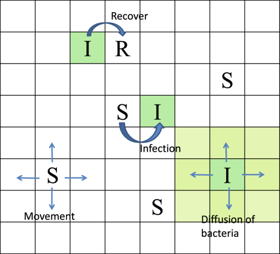
Structure of SIDW model for illustration of epidemic events, individuals movements and diffusion of bacteria (Color figure online)

Here we give our novel ideas on how to keep the individuals’ movement consistent with the spatial diffusion of the released pathogen and focus on the two following novelties: (i) coupling the spatial scales—the spatially shed pathogen from an infected individual should be linked to the dynamics of the pathogen described by the reaction–diffusion equation (4). In particular, given an infected individual $I_j$ releasing pathogen at the rate of ${\eta }_j$ at location x, the shed pathogen then follows the dynamics of model (4), and hence should be located in the grid associated with the spatial place x. (ii) Coupling the temporal scales—individuals’ movement should be linked to the spatial diffusion of the pathogen at the temporal scale. Note that the time of individuals’ movement is the number of iterations (Iter) with a step size of ($dt=1$), then we choose the step size for simulating the reaction–diffusive equation (4) as $\tau =T/\mathrm{Iter}$. The detailed algorithms are given in “Appendix A3”.

Modeling the Threshold Control Measures

Spatial control measures involve where to control or what the intensity of a control measure is. To address this, we assume that there exists a critical size of infected individuals, denoted by $I_{\mathrm{c}}$, such that we trigger the control measures (local isolation strategy or uniform isolation strategy) once the total number of infected individuals reaches the threshold $I_{\mathrm{c}}$. The general ODE model equation without considering spatial factor is as follows:

$$\begin{array}{c}\hfill \frac{\mathrm{d}Y}{\mathrm{d}t}=f(t,Y,\varrho (t)u(t)),\text{with}\varrho (t)=\left\{\begin{array}{cc}& 0,I\le I_{\mathrm{c}},\hfill \\ \hfill & 1,I>I_{\mathrm{c}},\hfill \end{array}\right)\end{array}$$ 5

where state variable $Y={(S,I,R)}^{\mathrm{T}}$ and a critical level of infection $I_{\mathrm{c}}(I_{\mathrm{c}}>0)$ determines whether a control measure, represented by u(t), is triggered or not. This threshold policy (hereafter named TP), which is a simple case of variable structure control in the control literature, has been successfully applied to pest management and disease control (Tang et al. 2012; Tang and Liang 2013; Xiao et al. 2013, 2015).

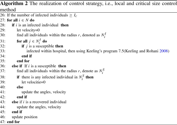
Local isolation strategy denotes the isolation of infected individuals within their cluster radius and also the limitation of the movement of susceptibles within the radius. Here, within the isolation area the infected individuals could release pathogen into the environment, which may infect susceptible individuals within the isolation area. Once an infected individual recovers, then he/she can move freely as before. This local isolation strategy resembles the Fengxiao strategy which was widely used in universities in China during the A/H1N1 pandemic influenza in 2009 (Tang et al. 2010). We give the detailed algorithms to realize the local control strategy in “Appendix A2”.

Uniform isolation strategy means that some common isolation areas (such as a hospital ) during the whole outbreak are used to isolate and treat infected individuals. With this measure, the infected individual, once diagnosed, is taken to (and stochastically set in) the common isolation area. Similarly, the isolated infected individuals cannot move into the common isolation area, but can shed pathogen. In contrast, the susceptible individuals can move freely in the common isolation areas and consequently may be infected, which calls for strong stringent disinfection measures in the common isolation areas.

Results

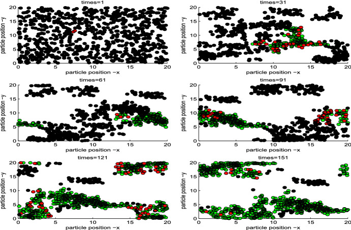
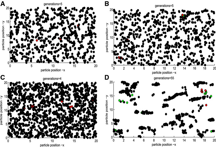
We simulate the transmission dynamics of an infectious disease while individuals are moving. Figure 2 illustrates the variation in both spatial position and infection status of individuals induced by a single infected individual at different times. It shows the whole process of the disease outbreak while individuals are moving and, in particular, during a disease outbreak individuals with the same infection status exhibit the property of clustering.

Fig. 2.

Spatial distribution of susceptible (black), infected (red) and recovered (green) individuals. Based on Keeling’s idea and considering the individual movement within a certain plane, i.e., the position of any individual could be dynamic as time varies . The parameter values are as follows: the total number of $N=763$ with spatial grid $[0,20]\times [0,20]$, $\beta =0.025,\alpha =3.5,\gamma =0.17$ and $I_0=1$ . The initial velocity $v_0=0.2$, the radius of nearest neighbor is $r=1$, the intensity of direction perturbation $\mathrm{\Delta }\theta =0.06$ with $\sigma =0.66$ (Color figure online)

Effect of Individuals’ Movements on Disease Specifics

In order to better evaluate the effects of spatial movement on the spread of disease, we take the mean $R_0$, final size and peak time as indices to show how the key parameters affect the disease spread. Here the basic reproduction number $R_0$ is the expected number of secondary infectious individuals generated by a single infected individual during his mean infectious period. To do this, the above indicators are obtained by means of the average over 200 simulations. We mainly focus on effects of the velocity of individuals’ movement ($V_0$), the radius of spatial infection (r) and the weight parameter ($\sigma$) on the above indicators and consider the following three cases:

Case A: Effect of velocity$V_0$on disease specifics We list the possible final sizes (RFN), peak timings, peak values for various velocities in Table 1. The results reveal that the individuals’ movement speed $V_0$ plays an important role in affecting the spread of infectious diseases. It shows that as the movement speed increases, the average $R_0$ will gradually increase. Note that when the moving speed is very low, for example $V_0=0.01$, the average $R_0$ is less than that for the classic SIR model without movement. That is because we assume that the infected individuals can only infect the susceptibles around them rather than all possible susceptibles. Thus, when the moving speed is very low, the neighborhood of infected people may not have a sufficient number of susceptibles. However, as the speed increases, i.e., the individuals’ aggregation is so fast that more susceptible individuals could be within the radius of an infected individual, resulting in an increase in mean $R_0$ and eventually the reproduction number mediated by individuals’ movement may be greater than that for the model without movement. Further, it follows from Table 1 that the higher the velocity $V_0$ is, the higher the final size, the higher the peak value and the earlier that the outbreak peaks. A relatively slow movement may result in multiple outbreaks, while quick movements lead to a single peak being more likely.

Table 1.

The effect of movement speed $V_0$ on the average indicators of interest

$V_0$	Mean $R_0$	Final size	Peak time	Peak value	Outbreaks
0.010	1.7500	35.0150	105	3.8350	Multiple
0.025	2.3000	105.7250	91	7.2650	Multiple
0.005	3.1700	264.6300	100	19.0250	Multiple
0.075	4.1400	411.7000	80	30.5250	Multiple
0.100	4.8950	535.7350	63	45.4450	Multiple
0.125	5.2200	583.8800	55	57.9850	Multiple
0.150	6.1350	635.9850	58	69.3250	Single
0.175	6.4050	657.4650	42	83.6400	Single
0.200	7.0450	683.0300	39	93.2650	Single

Case B: Effect of the radius of spatial infection r on disease specifics Note that the cluster radius could influence the individual behavior during the movement. In the following, we investigate variation in disease specifics with r for fixed velocity $V_0=0.05$, and list outcomes in Table 2. It follows that increasing the cluster radius r gradually decreases the average $R_0$, while the impacts of r on the final size, peak time and peak value seem to be non-monotonic and exhibit more complex patterns, which reveals that small variations in the cluster radius could result in significant changes in those indicators.

Table 2.

The effects of cluster radius r on the average indicators of interest

r	Mean $R_0$	Final size	Peak time	Peak value	Humps
0.20	4.2250	376.1200	102	63.2500	Single
0.30	4.1300	363.3850	99	37.4400	Multiple
0.40	3.6100	282.7750	108	21.9300	Multiple
0.50	3.1700	264.6300	100	19.0250	Multiple
0.60	2.9900	265.1750	91	15.6150	Multiple
0.70	2.7950	300.0350	83	17.3600	Multiple
0.80	2.7100	319.4850	93	18.7600	Multiple
0.90	2.6350	304.2050	98	19.8100	Multiple
1.00	2.5250	320.0100	113	20.8400	Multiple

Case C: Effect of weight parameter$\sigma$on disease specifics To investigate the effect of weight parameter $\sigma$ on the mean $R_0$ and outbreaks, we investigate variation in disease specifics with $\sigma$ for fixed $V_0=0.05,r=0.5$, and list outcomes in Table 3. It follows that increasing the weight parameter $\sigma$ greatly increases the average $R_0$, while the impacts of $\sigma$ on the final size, peak time and peak value exhibit non-monotonic and more complex patterns, indicating that small variations in parameter $\sigma$, associated with the level of following herd behavior, could result in significant changes in those indicators. This means that the lower the bandwagon effect is (i.e., the greater $\sigma$ ) the more new infections there are, which is because more individuals move in their own ways such that the infected individuals move to the wider areas and may infect more other susceptibles.

Table 3.

The effects of weight parameter $\sigma$ on the average indicators of interest

$\sigma$	Mean $R_0$	Final size	Peak time	Peak value	Humps
0.10	2.6750	273.1550	101	20.4800	Multiple
0.20	2.7300	262.5450	116	19.8050	Multiple
0.30	2.9150	281.3000	88	19.6900	Multiple
0.40	3.0900	257.2750	93	17.2250	Multiple
0.50	3.2800	253.4650	90	16.2850	Multiple
0.60	3.2600	259.5900	65	17.0600	Multiple
0.70	3.3500	285.2350	120	17.4250	Multiple
0.80	3.5950	331.5400	92	24.4600	Multiple
0.90	4.1150	410.6250	117	35.6750	Multiple

Impact of Local Control Measures (Spatial Threshold Policy) on the Spread of Disease

Here, we focus on effects of the critical size $I_{\mathrm{c}}$ and the number of initial infected individuals on the indicators discussed above. However, the actual control reproduction number is adopted, which is the average number of secondary infections induced by a single infected individual under the control strategies. The control reproduction number $R_0^c$ can be defined as follows:

$$\begin{array}{c}\hfill R_0^c=\frac{{\sum }_{j=1}^{I_{\mathrm{c}}}{R}_0^j}{I_{\mathrm{c}}},\end{array}$$

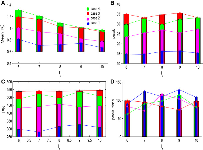
where $R_0^j$ represents the secondary infections induced by the j-th infected individual. We consider the following four cases: let the threshold level $I_{\mathrm{c}}=6,7,8,9,10$ with initial infected individuals $I_0=1$ (Case 1), $I_0=2$ (Case 2), $I_0=3$ (Case 3) and $I_0=3$ and allowing that any individual can slowly move in the isolation area (Case 4, and here $V_0^r=0.015$). Note that here the total number of infected people may not reach the critical size $I_{\mathrm{c}}$ for some simulations, and consequently control measures are not triggered at all. Another possible extreme case is that some infected individuals may not infect any susceptible individual during the whole simulation process, then we do not consider those extreme scenarios when we calculate the control reproduction number $R_0^c$.

Figure 3 shows the effects of threshold level $I_{\mathrm{c}}$ and initial data $I_0$ on the mean $R_0^c$ and other epidemic specifics. It follows from Fig. 3a that for a given initial data $I_0$, the $R_0^c$ shows the decline trend as $I_{\mathrm{c}}$ increases, which implies that the later the control strategy implements (greater value of $I_{\mathrm{c}}$) the lower the number of new infections (the lesser $R_0^c$). It seems unreasonable that early implementation of strategies induces more new infections. Bearing in mind that this isolation strategy does not only isolate the infected individuals but also the susceptibles who are within the cluster radius of the isolated infected individual. Then early implementation of control strategies usually brings about the clustering of outbreaks in local areas, and consequently induces more new infections, which was observed during the 2009 A/H1N1 pandemic influenza (Tang et al. 2010) when the Fengxiao strategy was implemented. Further, it shows that the mean $R_0^c$ in Case 4 is larger than that for Case 3 for all threshold levels $I_{\mathrm{c}}$, which implies that if the individuals in the isolation area can move slowly, then the mean reproduction number $R_0^c$ is greater than that for the case in which the individual cannot move.

Fig. 3.

Variation in mean $R_0$ and disease specifics with the threshold level $I_{\mathrm{c}}$ for four different cases. The baseline parameter values in this subsection are fixed as follows: $N=763$ with spatial grid $[0,20]\times [0,20]$, $\beta =0.025,\alpha =3.5,\gamma =0.17$, and $I_0=1$. $\mathrm{\Delta }=0.06,\sigma =0.66$ with $V_0=0.005$, cluster radius $r=0.5$ (Color figure online)

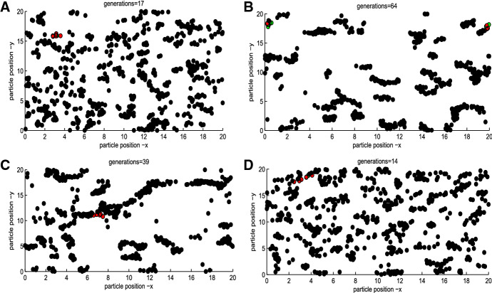
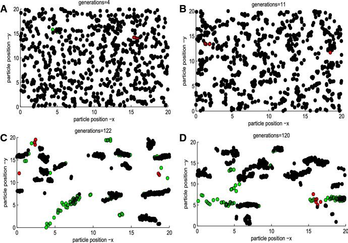
Further, Fig. 3a indicates that for a given threshold level $I_{\mathrm{c}}$ the mean $R_0^c$ will increase as $I_0$ increases. It seems odd that the mean reproduction number should be independent of the initial number of infected individuals. It is worth mentioning that the spatial distribution of individuals will vary with different initial numbers of infected individuals when the isolation strategy has been triggered (i.e., the threshold level $I_{\mathrm{c}}$ is reached), as shown in Figs. 10, 11 and 12 in “Appendix”. In particular, Figs. 10, 11 and 12 in “Appendix” show that the spatial heterogeneity becomes stronger when more infected individuals are introduced, then the isolated areas are distributed more broadly, and consequently more new infections are obtained (meaning greater mean value of $R_0^c$). It follows that the higher the number of initial infected individuals, the higher the peaks and the greater the final size, compared with Cases 1, 2 with 3 (or 4, as shown in Fig. 3b, c, and the earlier the outbreak peaks, as shown in Fig. 3d.

Fig. 10.

Spatial distribution of infected individuals with $I_0=1,I_{\mathrm{c}}=6$ (Color figure online)

Fig. 11.

Spatial distribution of infected individuals with $I_0=2,I_{\mathrm{c}}=6$ (Color figure online)

Fig. 12.

Spatial distribution of infected individuals with $I_0=3,I_{\mathrm{c}}=6$ (Color figure online)

Effects of Spatial Factors (Individuals’ Movements and Pathogen Diffusion) on the Disease Spread

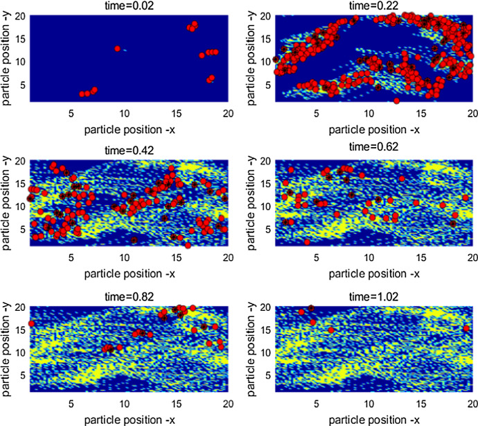
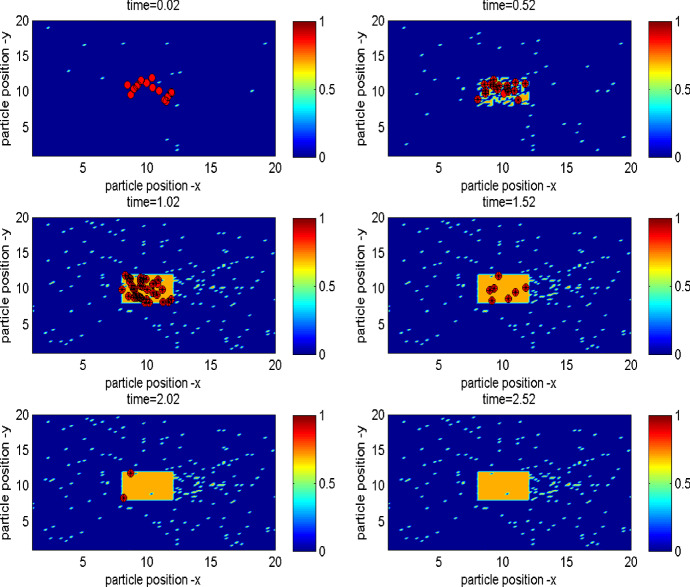
In order to further examine the impact of microscale infection/diffusion processes, we now extend our simulation model by linking the pathogen’s shedding/excretion, transmission and continuous diffusion to the epidemic process and random movement of individuals at the population level. We initially design the difference scheme of the reaction–diffusive equation (4) and then develop the method of coupling pathogens’ diffusion with individuals’ moving and transmission at spatiotemporal scales to do individual simulations at both the microscale and the macroscale. Similarly, we ran the algorithms 200 times and provide the mean incidence of disease infection over 200 times. Figure 4 reveals the dynamics of population infection, spatial movement of infected individuals and cumulative growth of pathogen over time. It also shows individuals with the same infection status showing the property of clustering.

Fig. 4.

Illustration of the infection dynamics, spatial movement of infected persons and cumulative growth of bacteria. Red circles represent the infected individuals and red circles with $\ast$ denote the individuals infected by bacteria, yellow dots represent the pathogens. The six subplots reveal the spatial distribution of pathogen growing and diffusion over time (Color figure online)

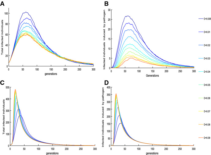
To investigate the effect of pathogen diffusion on disease spread, we plot the number of infected individuals versus time at various diffusion rates D, as shown in Fig. 5. It shows that a high diffusion rate of pathogen results in a decline in the total number of infected individuals and the number of infected individuals who are infected by pathogen (as shown in Fig. 5a, b). This implies that air flow (or air movement) is beneficial for disease control. A repeat of plotting the number of infected individuals with various dilution rates of pathogen $\mu$ reveals that the total number of infected individuals, the recovered population and peak values decrease as the $\mu$ increases. The plots are similar to Fig. 5 and we omit them. This reveals that frequent environmental clearance is beneficial for mitigating disease spread.

Fig. 5.

The effect of parameter D on the number of the infected (a, b) without pathogen growing in reservoir (c, d) with pathogen growing in reservoir given in (6) with $g=1,C=1$. The baseline parameter values are as follows: $\beta =0.025,\gamma =0.17,\alpha =3.5$, and the parameters for individual initial velocity $v_0=0.005,r=0.5$, the shading rate of i-th infected individual is ${\eta }_i=0.6$ with bacteria threshold ($w_0=0.4$). We choose the dispersal rate and cleaning rate for investigating the effects of bacteria on disease spread, where $I_0=5$ (Color figure online)

To further examine the influence of pathogens growing in the environment on outcomes, we repeat Fig. 5 with the dynamics of pathogens following

$$\begin{array}{c}\hfill \frac{\partial W(t,x)}{\mathrm{d}t}=\eta I(t,x)+gW(t,x)(1-cW(t,x))-(\mu +\nu N)W(t,x)+D\mathrm{\Delta }W.\\ \hfill \end{array}$$ 6

Here positive constants g and 1/c denote the grow rate and the carrying capacity, respectively. The plots shown in Fig. 5c, d illustrate that a high diffusion rate of pathogen leads to an increase in the total number of infected individuals and the number of infected individuals who are infected by pathogen, which implies that higher diffusion of pathogen, due to its ability of self-growing in reservoir, causes more contaminated places and induces more infected individuals. This indicated that inclusion of pathogens growing can induce a significant amplification in disease outbreaks with varying diffusion rates D, which agrees well with the existing results (Codeco 2001; Joh et al. 2009; Kong et al. 2014).

Impact of Control Tactics Associated with Immediate Isolation Once Diagnosed

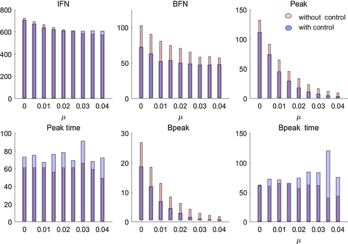
To investigate the effects of the rate of clearance $\mu$ and the control strategy on the disease spread, we illustrate the six epidemic indices including IFN (BFN)—the total number of infected individuals (who are infected by bacteria), peak (Bpeak)—the maximal number of infected individuals (who are infected by pathogen), peak time ( Bpeak time)—the time that the maximal number of infected individuals (who are infected by pathogen) is reached, as shown in Fig. 6. It follows from Fig. 6 that increasing the rate of clearance greatly reduced the BFN and Bpeak, as expected, indicating that environmental cleaning is effective in lowering infections via free-living pathogen in the contaminated environment. It also shows that taking the local isolation measure does not influence the changing trend of BFN, Peak and Bpeak with varying parameter $\mu$, but results in lower values of BFN, peak and Bpeak and later peaks. That is because the local isolation measure limits movement of infected and susceptible individuals, and then leads to a low level of infections.

Fig. 6.

Variation in disease specifics with the rate of clearance for the simulation model with and without local isolation measures over 200 simulations. IFN (BFN)—the total number of infected individuals (who are infected by bacteria), peak (Bpeak)—the maximal number of infected individuals (who are infected by bacteria), peak time (Bpeak time)—the time that the maximal number of infected individuals (who are infected by bacteria) is reached (Color figure online)

To further investigate the effect of the uniform isolation strategy with various sizes of control areas, we simulate the proposed model with an isolation region to examine disease specifics (IFN, BFN peak and etc). Without loss of generality, we assume that there is a rectangular area in the centre of the whole considered space, in which the infected individuals are isolated, as shown in Fig. 13, which reveals the epidemic process, individuals’ movement and pathogens’ diffusion under the uniform isolation measure. Here we consider the following four cases:

Fig. 13.

Illustration of the infection dynamics, movement and uniform isolation strategy. Black and green dots represent susceptible and recovered individuals, respectively, red dots represent individuals infected either by infected individuals or by the pathogen, purple dots denote individuals infected by bacteria, light-blue dots indicate individuals recovering from pathogen infection (Color figure online)

Case u1 (or u2) Let $I_0=5$ and the isolation region is a rectangle of $[9,11]\times [9,11]$ (or $[8,12]\times [8,12])$;

Case u3 (or u4) Let $I_0=20$ and the isolation region is a rectangle of $[9,11]\times [9,11]$ (or $[8,12]\times [8,12]$);

Again, we run the algorithms 200 times and provide the mean incidence of disease infection over 200 times. Figures 7 and 8 show the results on disease specifics of Case u1 with Case u2 and those of Case u3 with Case u4. These results indicate that the common control region with relatively large size leads to an increase in IFN, BFN, peak and Bpeak and late peaks. In particular, Fig. 7 shows that for low values of $\mu$ the IFN and BFN for Case u1 are smaller than those for Case u2, while for high values of $\mu$ the IFN and BFN for Case u1 are greater than those for Case u2. This implies that with frequent clearance of the environment the uniform isolation strategy with a large control region leads to the total number infected individuals decline, which suggests that a large-scale isolation strategy with frequent clearance of the environment is beneficial for disease control. Figure 8 shows the similar trend of variation in disease specifics with varying the rate of clearance $\mu$, and moreover it exhibits large and late peaks when more initial infected individuals are introduced in the numerical simulations. It also follows from Figs. 7 and 8 that the uniform isolation strategy with larger size could postpone the peaks but with higher peak values.

Fig. 7.

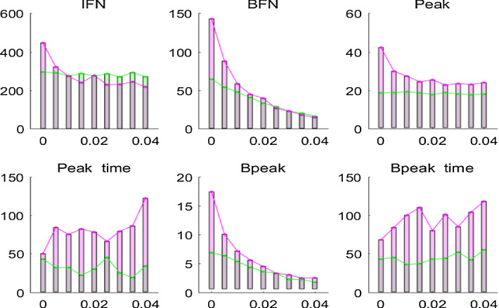
Variation in disease specifics with the rate of clearance for Case u1 (green) and Case u2 (red) under uniform isolation strategy. Diffusion rate of bacteria is $D=0.005$ (Color figure online)

Fig. 8.

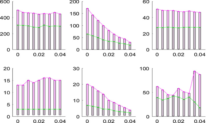
Variation in disease specifics with the rate of clearance for Case u3 (green) and Case u4 (red) under a uniform isolation strategy. Diffusion rate of bacteria is $D=0.005$ (Color figure online)

In order to compare the uniform isolation strategy (Case u1 and Case u3) with local isolation measures we again plot the disease specifics including IFN, BFN, Peak etc., with various $\mu$, as shown in Fig. 9. A relatively large rate of clearance of the pathogen leads to lower infections with the local isolation strategy than for those with the uniform isolation strategy. However, the uniform isolation strategy results in lower values of IFN, with small and early peaks for any rate of clearance. That is because under a local isolation strategy more aggregated outbreaks within the isolated areas may happen, inducing more total infections. This points to the advantages of the uniform isolation measure (or large-scale isolation strategy).

Fig. 9.

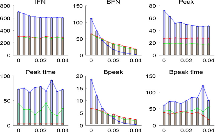
Variation in disease specifics with the rate of clearance for the local isolation strategy (blue), uniform isolation strategy (Case u1 (green), Case u3) (red). Diffusion rate of bacteria is $D=0.005$ (Color figure online)

Conclusion and Discussion

Mathematical modeling is an essential tool to achieve a system-level understanding of pathogen replication, spread and disease transmission at the population level. There are many challenges to coupling deterministic and stochastic simulations of discrete entities constituting the linkage of the macroscale to the microscale at temporal or spatial scales. Although IBMs have suffered from notable limitations including computational expense, but with more programming expertise and synthesis of different spatiotemporal scales (Yu and Bagheri 2016), they can record critical information for each individual such as by whom a person was infected, when he/she got infected and at which infection age an infected individual infected others. In this study, we develop an algorithm to simulate how individuals transmit infectious diseases to others and may release pathogens into the environment while moving, and vice versa these free-living pathogens can further infect individuals while dispersing, e.g., MRSA (Methicillin-resistant Staphylococcus aureus) and MRAB (multidrug-resistant Acinetobacter baumannii) transmissions in hospital infections (Wang et al. 2012, 2015; Wang and Tang 2017). We link individual random movements to pathogen’s continuous diffusion, link the slow dynamics for disease transmission at the population level to the fast dynamics for pathogen shedding/excretion at the individual level, in order to examine effects of the individuals’ movements, pathogen’s diffusion and spatial control measures on the disease outbreak. It is a systematic analysis of the effects of individual random walk in space, pathogen’s diffusion, disease transmission (directly or indirectly via the pathogen) and threshold control policy on the transmission of infectious diseases.

Numerical simulations indicate that during a disease outbreak individuals in the same infection status show the property of clustering and, in particular, individuals’ quick movements lead to an increase in the average reproduction number $R_0$, final size and the peak value. Increasing the cluster radius r decreases the average $R_0$, while the weight parameter $\sigma$, associated with the level of autonomous mobility, increases the average $R_0$. This indicates that the more the bandwagon effect is (i.e., the lower $\sigma$ ) the fewer the new infections, which is because more individuals get together such that disease transmission becomes difficult due to lack of susceptibles.

Note that here increasing moving velocity leads to an increase in the average reproduction number $R_0$, which is opposed to most of previous works in which the basic reproduction number $R_0$ is decreasing with respect to the diffusion coefficient based on the reaction–diffusion equations (Allen et al. 2008; Peng 2009; Peng and Liu 2009; Peng and Yi 2013; Pang and Xiao 2019). It seems reasonable that strengthening diffusion increases disease transmission and hence is harmful for disease control, as suggested by our results and by the recent work on SEIR-type model reaction–diffusion model (Song et al. 2019). The disagreement on effect of diffusion on $R_0$ between our result and previous works is because individuals movement in our simulation has a kind of direction and is also mediated by population’s movement direction, rather than random diffusion represented by the reaction–diffusion equations.

Given the local isolation strategy under a threshold policy, we found for a given initial datum $I_0$, the mean control reproduction number $R_{\mathrm{c}}$ shows the decline trend as $I_{\mathrm{c}}$ increases, while for a given threshold level $I_{\mathrm{c}}$, the mean $R_{\mathrm{c}}$ will increase as $I_0$ increases. This indicates that the earlier the control strategy is implemented (lower value of $I_{\mathrm{c}}$) the more new infections there are (the more $R_{\mathrm{c}}$), which is in agreement with results of Tang et al. (2010) in which an early Fengxiao strategy induced more local A/H1N1 cases. That is because this early local strategy may lead to aggregated outbreaks within the isolated areas. Moreover, the more the initial infected individuals are introduced (the greater $I_0$), the stronger the spatial heterogeneity is when control is implemented, and hence the more new infections there are. This indicates that high level of spatial heterogeneity of seeded infection is a risk factor that induces new infections and large outbreak.

When considering the pathogens’ dynamics, we treat them deterministically due to the high rates of the shedding, diffusion and frequent cleaning of the environment, and hence the variation of the pathogen index is described by a reaction–diffusion equation. We found that either a high diffusion rate of the pathogen or frequent environmental clearance leads the total number of infected individuals to decline, which implies that air movement and frequent cleaning are beneficial for mitigating an outbreak. We further investigated the effect of a uniform isolation strategy on disease outbreaks and obtained that with frequent clearance of the environment a large size of the uniform isolation region results in a small final size, indicating that a large-scale isolation strategy with frequent clearance of environment is beneficial for disease control. By comparing the local and uniform isolation strategies, we obtained that the uniform isolation strategy leads to lower values of IFN, and peaks, suggesting the advantages of the uniform isolation (or large-scale isolation) strategy.

This study developed a multiscale model and the corresponding simulation method by linking individual movements to pathogen’s diffusion, linking the slow dynamics for disease transmission at the population level to the fast dynamics for pathogen shedding/excretion at the individual level. Some interesting and realistic conclusions, especially the efficacy of various control strategies on disease infection, were suggested. However, it is challenging to test the control measures by specific diseases due to lack of reliable data on the concentration of pathogen with/without diffusion, and we leave this for future work. We note also that our transmission simulation is based on a neighbor principle, that is, an infected individual can only infect susceptible individuals within a certain radius, which is a reasonable but ignoring contact network structure. Meanwhile we acknowledge that complex contact network structure greatly influences on disease infection (Sun et al. 2018; Xiao et al. 2011; Shirley and Rushton 2005) and we leave this for future research.

Appendix

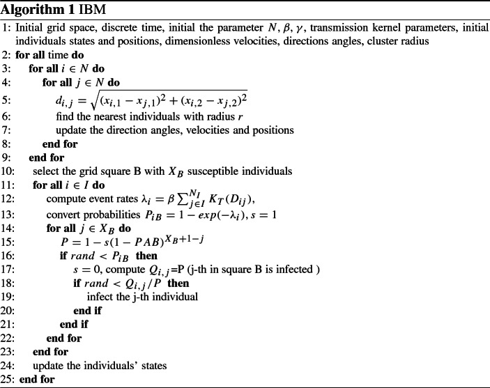
In the appendix, we provide the ideas of how to realize the disease transmission while individuals’ movement and pathogen’s diffusion, and give the detailed framework of algorithms proposed in this manuscript (Figs. 10, 11, 12, 13).

Appendix A1: Framework of Algorithm of the Epidemic Model with Individuals’ Movement

Appendix A2: Framework of Algorithm for the Model with Local Isolation Strategies

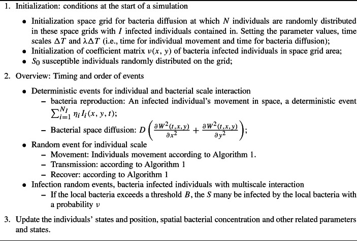
Appendix A3: Framework of Algorithm for Coupling Pathogens’ Diffusion with Individuals’ Movement

In this part, we initially give the details of the difference scheme of reaction–diffusive equation 4. For the diffusion term, we use the ADI (alternating-direction implicit) method to solve the diffusion equation. The ADI scheme provides a feasible method for solving the parabolic equations in 2-spatial dimensions by using tri-diagonal matrices. To do this, each time increment is executed in two steps.

In order to solve the diffusive-bacteria model, we first mesh the region. Considering a two-dimensional square space $L\times L$, and the time is T. Given isometric subdivision, we choose two positive integers M, N, let $h=L/M,\tau =T/N,x_p=ph,y_q=qh(0\le p,q\le M),t_n=n\tau (0\le n\le N),0=x_0<x_1<\cdots <x_M=L,0=y_0<y_1<\cdots <y_M=L,0=t_0<t_1<\cdots <t_N<T$, the space increment is $h=x_{p+1}-x(p)=y(q+1)-y(q)(p,q=0,1,\dots ,M-1)$, and time increment is $\tau =t_{n+1}-t_n(n=0,1,\dots ,N-1)$. We divide the space-time domain into a cube grid, and the lattice point is $(x_p,y_q,t_n)$, then the function $w_{p,q}^n$ will be approximation to the solution of Eq. 4 at the point $(x_p,y_q,t_n)$.

We introduce the transition layer $n+1/2$, there are two steps from n to $n+1$: For the first step, from n to $n+1/2$, we use an implicit difference scheme in the x direction and an explicit difference scheme in the y direction. Then we have:

$$\begin{array}{c}\hfill \begin{array}{ccc}\hfill \frac{W_{p,q}^{n+1/2}-W_{p,q}^n}{\tau /2}& =& D\left(\frac{W_{p+1,q}^n-2W_{p,q}^n+W_{p-1,q}^n}{h^2},+,\frac{W_{p,q+1}^{n+1/2}-2W_{p,q}^{n+1/2}+W_{p,q-1}^{n+1/2}}{h^2}\right)\hfill \\ \hfill & & -(\mu +\nu N)W_{p,q}^n+\sum _{i=1}^{N_I}{\eta }_{i}I{{}_i}_{p,q}^{n+1/2}\hfill \end{array}\end{array}$$ 7

Let $\zeta =\frac{\tau D}{2h^2}$ in the above equation, then we get

$$\begin{array}{c}\hfill \begin{array}{ccc}\hfill \zeta W_{p,q-1}^{n+1/2}+(1+2\zeta )W_{p,q}^{n+1/2}-\zeta W_{p,q+1}^{n+1/2}& =& \zeta W_{p-1,q}^n+(1-2\zeta -\tau /2(\mu +\nu N))W_{p,q}^n\hfill \\ \hfill & & +\zeta W_{p+1,q+1}^n+\tau /2\sum _{i=1}^{N_I}{\eta }_{i}I{{}_i}_{p,q}^{n+1/2}\hfill \end{array}\end{array}$$ 8

which is explicit.

For the second step, from $n+1/2$ to n, we use an explicit difference scheme in the x direction and an implicit difference scheme in the y direction. Then we obtain the following equation:

$$\begin{array}{c}\hfill \begin{array}{ccc}\hfill \frac{W_{p,q}^{n+1}-W_{p,q}^{n+1/2}}{\tau /2}& =& D\left(\frac{W_{p+1,q}^{n+1}-2W_{p,q}^{n+1}+W_{p-1,q}^{n+1}}{h^2},+,\frac{W_{p,q+1}^{n+1/2}-2W_{p,q}^{n+1/2}+W_{p,q-1}^{n+1/2}}{h^2}\right)\hfill \\ \hfill & & -(\mu +\nu N)W_{p,q}^{n+1/2}+\sum _{i=1}^{N_I}{\eta }_{i}I{{}_i}_{p,q}^{n+1/2}\hfill \end{array}\end{array}$$ 9

Similarly, we let $\zeta =\frac{\tau D}{2h^2}$ and rearrange the above equation, then we get

$$\begin{array}{c}\hfill \begin{array}{cc}& -\zeta W_{p-1,q}^{n+1}+(1+2\zeta )W_{p,q}^{n+1}-\zeta W_{p,q-1}^{n+1}\hfill \\ \hfill & =\zeta W_{p,q-1}^{n+1/2}+(1-2\zeta -\tau /2(\mu +\nu N))W_{p,q}^{n+1/2}\hfill \\ \hfill & +\zeta W_{p,q+1}^{n+1/2}+\tau /2\sum _{i=1}^{N_I}{\eta }_{i}I{{}_i}_{p,q}^{n+1/2}\hfill \end{array}\end{array}$$ 10

which is implicit.

The boundary conditions for the problem are approximately by $W_{1,0:M}=W_{M,0:M}$; $W_{0:M,1}=W_{0:M,M}$.

Appendix A3: Framework of Algorithm of SIRW Model

References

- Allen LJS, Bolker BM, Lou Y, Nevai AL. Asymptotic profiles of the steady states for an SIS epidemic reaction–diffusion model. Discrete Contin Dyn Syst Ser A. 2008;21(1):1–20. [Google Scholar]
- Anderson RM, May RM. Infectious diseases of humans: dynamics and control. Oxford: Oxford University Press; 1991. [Google Scholar]
- Bauer AL, Beauchemin CA, Perelson AS. Agent-based modeling of host-pathogen systems: the successes and challenges. Inf Sci. 2009;179:1379–1389. doi: 10.1016/j.ins.2008.11.012. [DOI] [PMC free article] [PubMed] [Google Scholar]
- Codeco CT. Endemic and epidemic dynamics of cholera: the role of the aquatic reservoir. BMC Infect Dis. 2001;1(1):1. doi: 10.1186/1471-2334-1-1. [DOI] [PMC free article] [PubMed] [Google Scholar]
- Dorratoltaj N, Nikin-Beers R, Ciupe SM, et al. Multi-scale immunoepidemiological modeling of within-host and between-host HIV dynamics: systematic review of mathematical models. Peer J. 2017 doi: 10.7717/peerj.3877. [DOI] [PMC free article] [PubMed] [Google Scholar]
- Diekmann O, Heesterbeek JAP. Mathematical epidemiology of infectious diseases: model building. Analysis and interpretation. New York: Wiley; 2000. [Google Scholar]
- Feng ZL, Velasco-Hernandez JX, Tapia-Santos B, Leite MC. A model for coupling within-host and between-host dynamics in an infectious disease. Nonlinear Dyn. 2012;68:401–411. [Google Scholar]
- Feng ZL, Hernandez JV, Santos BT. A mathematical model for coupling within-host and between-host dynamics in an environmentally-driven infectious disease. Math Biosci. 2013;241:49–55. doi: 10.1016/j.mbs.2012.09.004. [DOI] [PubMed] [Google Scholar]
- Gandolfi A, Pugliese A, Sinisgalli C. Epidemic dynamics and host immune response: a nested approach. J Math Biol. 2014;70:399–435. doi: 10.1007/s00285-014-0769-8. [DOI] [PubMed] [Google Scholar]
- Garira W. A complete categorization of multiscale models of infectious disease systems. J Biol Dyn. 2017;11:378–435. doi: 10.1080/17513758.2017.1367849. [DOI] [PubMed] [Google Scholar]
- Garira W. A primer on multiscale modelling of infectious disease systems. Infect Dis Model. 2018;3:176–191. doi: 10.1016/j.idm.2018.09.005. [DOI] [PMC free article] [PubMed] [Google Scholar]
- Gillespie DT. A general method for numerically simulating the stochastic time evolution of coupled chemical reactions. J Comput Phys. 1976;22:403–434. [Google Scholar]
- Gillespie DT. Exact stochastic simulation of coupled chemical reactions. J Phys Chem. 1977;81:2340–2361. [Google Scholar]
- Gog JR, Pellis L, Wood JL, et al. Seven challenges in modeling pathogen dynamics within-host and across scales. Epidemics. 2015;10:45–48. doi: 10.1016/j.epidem.2014.09.009. [DOI] [PubMed] [Google Scholar]
- Hosseini I, Gabhann FM. Multi-scale modeling of HIV infection in vitro and APOBEC3g-based anti-retroviral therapy. PLoS Comput Biol. 2012;8:e1002371. doi: 10.1371/journal.pcbi.1002371. [DOI] [PMC free article] [PubMed] [Google Scholar]
- Joh RI, Wang H, Weiss H, Weitz JS. Dynamics of indirectly transmitted infectious diseases with immunological threshold. Bull Math Biol. 2009;71(4):845–862. doi: 10.1007/s11538-008-9384-4. [DOI] [PubMed] [Google Scholar]
- Keeling MJ, Rohani P. Modeling infectious diseases in humans and animals. Princeton: Princeton University Press; 2008. [Google Scholar]
- Kong JD, Davis W, Li X, Wang H. Stability and sensitivity analysis of the iSIR model for indirectly transmitted infectious diseases with immunological threshold. SIAM J Appl Math. 2014;74(5):1418–1441. [Google Scholar]
- Luo J, Wang J, Wang H. Seasonal forcing and exponential threshold incidence in cholera dynamics. Discrete Contin Dyn Syst Ser B. 2017;22(6):2261. [Google Scholar]
- Murillo LN, Murillo MS, Perelson AS. Towards multiscale modeling of influenza infection. J Theor Biol. 2013;332:267–290. doi: 10.1016/j.jtbi.2013.03.024. [DOI] [PMC free article] [PubMed] [Google Scholar]
- Mukandavire Z, Liao S, Wang J, Gaff H, Smith DL, Morris JG. Estimating the reproductive numbers for the 2008–2009 cholera outbreaks in Zimbabwe. PNAS. 2011;108(21):8767–8772. doi: 10.1073/pnas.1019712108. [DOI] [PMC free article] [PubMed] [Google Scholar]
- Nowak M, May RM. Virus dynamics: mathematical principles of immunology and virology. Oxford: Oxford University Press; 2000. [Google Scholar]
- Pang D, Xiao Y. The SIS model with diffusion of virus in the environment. Math Biosci Eng. 2019;259:8–25. doi: 10.3934/mbe.2019141. [DOI] [PubMed] [Google Scholar]
- Peaceman DW, Rachford HH. The numerical solution of parabolic and elliptic differential equations. J Soc Ind Appl Math. 1995;3:28–41. [Google Scholar]
- Peng R. Asymptotic profiles of the positive steady state for an SIS epidemic reaction–diffusion model. Part I. J Differ Equ. 2009;247(4):1096–1119. [Google Scholar]
- Peng R, Liu S. Global stability of the steady states of an SIS epidemic reaction–diffusion model. Nonlinear Anal. 2009;71(1C2):239–247. [Google Scholar]
- Peng R, Yi F. Asymptotic profile of the positive steady state for an SIS epidemic reaction–diffusion model: effects of epidemic risk and population movement. Physica D. 2013;259:8–25. [Google Scholar]
- Rohani P, Breban R, Stallknecht DE, Drake JM. Environmental transmission of low pathogenicity avian influenza viruses and its implications for pathogen invasion. PNAS. 2009;106(25):10365–10369. doi: 10.1073/pnas.0809026106. [DOI] [PMC free article] [PubMed] [Google Scholar]
- Shen M, Xiao Y, Rong L. Global stability of an infection-age structured HIV-1 model linking within-host and between-host dynamics. Math Biosci. 2015;263:37–50. doi: 10.1016/j.mbs.2015.02.003. [DOI] [PubMed] [Google Scholar]
- Shirley MD, Rushton SP. The impacts of network topology on disease spread. Ecol Complex. 2005;2:287–99. [Google Scholar]
- Song P, Lou Y, Xiao Y. A spatial SEIRS reaction-diffusion model in heterogeneous environment. J Differ Equ. 2019;267:5084–5114. [Google Scholar]
- Sun X, Xiao Y, Tang S, Peng Z, Wu J, Wang N. Early HAART initiation may not reduce actual reproduction number and prevalence of MSM infection: perspectives from coupled within- and between-host modelling studies of Chinese MSM populations. PLoS ONE. 2016;11:1–21. doi: 10.1371/journal.pone.0150513. [DOI] [PMC free article] [PubMed] [Google Scholar]
- Sun X, Xiao Y, Peng Z, Wang N. Frequent implementation of interventions may increase HIV infections among MSM in China. Sci Rep. 2018;8(1):1–11. doi: 10.1038/s41598-017-18743-7. [DOI] [PMC free article] [PubMed] [Google Scholar]
- Tang S, Liang J. Global qualitative analysis of a non-smooth Gause predator-prey model with a refuge. Nonlinear Anal TMA. 2013;76:165–180. [Google Scholar]
- Tang S, Xiao Y, Yang Y, et al. Community-based measures for mitigating the 2009 H1N1 pandemic in China. PLoS ONE. 2010;5:e10911. doi: 10.1371/journal.pone.0010911. [DOI] [PMC free article] [PubMed] [Google Scholar]
- Tang S, Liang J, Xiao Y, Cheke RA. Sliding bifurcations of Filippov two stage pest control models with economic thresholds. SIAM J Appl Math. 2012;72:1061–1080. [Google Scholar]
- Tien JH, Earn DJ. Multiple transmission pathways and disease dynamics in a waterborne pathogen model. Bull Math Biol. 2010;72(6):1506–1533. doi: 10.1007/s11538-010-9507-6. [DOI] [PubMed] [Google Scholar]
- Wang X, Tang S. A multiscale model on hospital infections coupling macro and micro dynamics. Commun Nonlinear Sci Numer Simul. 2017;50:256–270. [Google Scholar]
- Wang X, Xiao Y, Wang J, et al. A mathematical model of effects of environmental contamination and presence of volunteers on hospital infections in China. J Theor Biol. 2012;293:161–173. doi: 10.1016/j.jtbi.2011.10.009. [DOI] [PubMed] [Google Scholar]
- Wang X, Chen Y, Zhao W, et al. A data-driven mathematical model of multi-drug resistant Acinetobacter baumannii transmission in an intensive care unit. Sci Rep. 2015;5:9478. doi: 10.1038/srep09478. [DOI] [PMC free article] [PubMed] [Google Scholar]
- Xiao Y, Zhou Y, Tang S. Modelling disease spread in dispersal networks at two levels. Math Med Biol. 2011;28:227–244. doi: 10.1093/imammb/dqq007. [DOI] [PubMed] [Google Scholar]
- Xiao Y, Zhao T, Tang S. Dynamics of an infectious diseases with media/psychology induced non-smooth incidence. Math Biosci Eng. 2013;10:445–461. doi: 10.3934/mbe.2013.10.445. [DOI] [PubMed] [Google Scholar]
- Xiao Y, Tang S, Wu J. Media impact switching surface during an infectious disease outbreak. Sci Rep. 2015;5:7838. doi: 10.1038/srep07838. [DOI] [PMC free article] [PubMed] [Google Scholar]
- Yu JS, Bagheri N. Multi-class and multi-scale models of complex biological phenomena. Curr Opin Biotechnol. 2016;39:167–173. doi: 10.1016/j.copbio.2016.04.002. [DOI] [PubMed] [Google Scholar]