Are 2D fingerprints still valuable for drug discovery?

Abstract

Recently, molecular fingerprints extracted from three-dimensional (3D) structures using advanced mathematics, such as algebraic topology, differential geometry, and graph theory have been paired with efficient machine learning, especially deep learning algorithms to outperform other methods in drug discovery applications and competitions. This raises the question of whether classical 2D fingerprints are still valuable in computer-aided drug discovery. This work considers 23 datasets associated with four typical problems, namely protein-ligand binding, toxicity, solubility and partition coefficient to assess the performance of eight 2D fingerprints. Advanced machine learning algorithms including random forest, gradient boosted decision tree, single-task deep neural network and multitask deep neural network are employed to construct efficient 2D-fingerprint based models. Additionally, appropriate consensus models are built to further enhance the performance of 2D-fingerprintbased methods. It is demonstrated that 2D-fingerprint-based models perform as well as the state-of-the-art 3D structure-based models for the predictions of toxicity, solubility, partition coefficient and protein-ligand binding affinity based on only ligand information. However, 3D structure-based models outperform 2D fingerprint-based methods in complex-based protein-ligand binding affinity predictions.

I. Introduction

Drug discovery is a multi-parameter optimization process, which involves a long list of chemical, biological, and physiological properties¹. For a drug candidate, numerous drug-related properties must be assessed, including binding affinity, toxicity, octanol-water partition coefficient (Log P), aqueous solubility (Log S), etc. Binding affinity assesses the strength of a drug’s binding to its target^2,3, while, toxicity is a measure of the degree to which a chemical compound can damage an organism adversely⁴. In addition, a partition coefficient is defined as the ratio of concentrations of a solute in a mixture of two immiscible solvents at equilibrium and, in the case of log P, represents the drug-relatedness of a compound as well as its hydrophobic effect on human bodies⁵. Another relevant drug attribute is aqueous solubility which plays a vital role in distribution, absorption, and biological activity, among other processes because 65–90 % of body mass is water^6,7. Their importance to drug design and discovery has been emphasized by many recent surveys^8,9. Indeed, unsatisfactory toxicity or pharmacokinetic properties are responsible for approximately half of drug candidate failures to reach the market¹⁰.

Traditional experiments for measuring drug properties are conducted either in vivo or in vitro. Such experiments are quite time consuming and expensive. Additionally, testing with animals can raise important ethical concerns. Therefore, various computer-aided or in silico methods become more attractive since they can produce quick results without sacrificing much accuracy in many situations. Among them, one of the most popular approaches is the quantitative structure-activity/property relationship (QSAR/QSPR) analysis. It assumes that similar molecules have similar bioactivities or physicochemical properties¹¹. Based on this assumption, activities and properties of new molecules can be predicted by studying the correlation between chemical or structural features of molecules and their activities or properties, reducing the need for time-consuming experiments.

Molecular fingerprints are one way of encoding the structural features of a molecule. They play a fundamental role in QSAR/QSPR analysis, virtual screening, similarity-based compound search, target molecule ranking, drug ADMET prediction, and other drug discovery processes. Molecular fingerprints are property profiles of a molecule, usually in the form of vectors with each vector element indicating the existence, the degree or the frequency of one particular structure feature^12–14. Various fingerprints have been developed for molecular feature encoding in the past few decades^15–17. Most fingerprints are 2D fingerprints which can be extracted from molecular connection tables without 3D structure information. However, high dimensional fingerprints have also been developed to utilize 3D molecular structure and other information¹⁸.

There are four main categories of 2D fingerprints, namely substructure key-based fingerprints, topological or path-based fingerprints, circular fingerprints, and pharmacophore fingerprints. Substructure key-based fingerprints are bit strings representing the presence of certain substructures or fragments from a given list of structural keys in the compound. Molecular access system (MACCS)¹⁹ is one of the most popular substructure key-based fingerprint methods. Topological or path-based fingerprints are based on analyzing all the fragments of a molecule following a (usually linear) path up to a certain number of bonds, and then hashing every one of these paths to create one fingerprint. The most prominent ones in this category are FP2²⁰, Daylight²¹ and electro-topological state (Estate)²² fingerprints. Circular fingerprints are also hashed topological fingerprints but rather than looking for paths in a molecule, they record the environment of each atom up to a pre-determined radius. A well-known example for this class is extended-connectivity fingerprint (ECFP)¹⁵. Pharmacophore fingerprints include the relevant features and interactions needed for a molecule to be active against a given target, including 2D-pharmacophore²³, 3D-pharmacophore²⁴ and extended reduced graph (ERG)²⁵ fingerprints as examples. Since 2D fingerprints only rely on the 2D structures, their generation is easy, fast and convenient.

In addition to the four categories mentioned above, recent improvements in deep learning have enabled the creation of neural fingerprints^26,27-where the mapping between fingerprints and 2D structures is learned simultaneously with the parameters of the regression/classification model that maps fingerprints to targets. These ‘learned’ fingerprints can potentially improve predictive performance on QSAR/QSPR tasks, but they must be relearned when trying to predict new properties across significantly different regions of chemical space. Since the focus of this work is on comparing 2D and 3D descriptors across a number of disparate tasks and chemically diverse datasets, we have chosen not to consider neural fingerprints.

Most commonly used 2D molecular fingerprints were derived over a decade ago and their validation was carried out using classical regression or classification algorithms, such as linear regression, logistic regression, logistic classification, naive Bayes, k-nearest neighbors, support vector machine, etc. On the other hand, new 3D structure-based fingerprints built from algebraic topology^28,29, differential geometry³⁰, geometric graph theory^31,32, and algebraic graph theory³³ have been developed in recent years. In particular, these new fingerprints were mostly paired with advanced machine learning algorithms, such as random forest (RF)³⁴, gradient boosting decision tree (GBDT)³⁵, single-task deep neural networks (ST-DNNs)³⁶, multi-task deep neural networks (MT-DNNs)³⁷, convolutional neural network (CNN), recurrent neural network (RNN), etc. methodology, which are now easily accessible to the scientific community via user-friendly deep learning frameworks in popular programming languages^38,39. Often, these new methods have demonstrated higher accuracy or better performance than earlier methods in the literature, which are typically based on 2D fingerprints and/or simple machine learning algorithms for drug discovery related applications, such as protein-ligand binding²⁸, virtual screening²⁹, toxicity⁴, solubility⁵, partition coefficient⁵, as well as protein folding stability change upon mutation⁴⁰. Additionally, recent results from D3R Grand Challenges, a community-wide annual competition series in computer-aided drug design, indicate that structure-based methods using sophisticated 3D structure-based fingerprints have an advantage over ligand-based methods using 2D fingerprints in scoring and free energy predictions^33,41. These developments raise an interesting question of whether 2D fingerprints are still valuable for drug design and discovery. Therefore, there is pressing need to reassess 2D fingerprints with advanced machine learning algorithms and compare their performance with the state-of-the-art 3D structure-based fingerprints for drug discovery related applications.

The objective of the present work is to reassess the predictive power of eight popular 2D fingerprints for four important drug-related problems, namely, toxicity, binding affinity, Log P, and Log S, involving a total of 23 datasets. These problems are selected for the availability of reference results generated by the state-of-the-art 3D structure-based fingerprints in the literature. To optimize 2D fingerprints’ performance, advanced machine learning algorithms, including RF, GBDT, ST-DNN, and MT-DNN, are employed in the present study. Additionally, consensus models are constructed from appropriate combinations of 2D fingerprint-based predictions to further enhance their performance. The predictive power of each 2D fingerprint for certain functional groups is analyzed. Extensive numerical studies over 23 datasets using eight 2D fingerprints and four different machine learning algorithms indicate that the combination of appropriate machine learning algorithms and 2D fingerprint-based models, particularly consensus models, can bring significant improvements over previous 2D QSPR approaches especially on toxicity predictions⁴². Moreover, 2D fingerprint-based models perform as well as the state-of-the-art 3D structure-based fingerprints in the predictions of toxicity, solubility, partition coefficient and ligand-based protein-ligand binding affinity. Finally, topology-based fingerprints extracted from 3D protein-ligand complexes have a significant advantage over 2D fingerprints in complex-based protein-ligand binding affinity predictions. This is because 2D models can only take care of relatively simple geometry, so do not work well for macromolecules that have complex 3D structures⁴³. We believe that the present performance analysis and assessment will provide a useful guideline on how to choose appropriate fingerprints and machine learning methods for drug discovery related applications.

II. Methods

II.A. 2D fingerprints

In the present work, we investigate eight popular 2D fingerprints, including FP2 fingerprint, MACCS fingerprint, Daylight fingerprint, Estate1 fingerprint, Estate2 fingerprint, ECFP4 Fingerprint, 2D-pharmacophore (Pharm2D), and extended reduced graph fingerprint (ERG). They are chosen to represent four main 2D molecular fingerprint categories, namely key-based fingerprints, topological or path-based fingerprints, circular fingerprints, pharmacophore fingerprints. These features are some of the most popular and commonly used ones. Table 1 summarizes the information related to these fingerprints. All 2D fingerprints were generated by Openbabel (version 2.4.1)²⁰ and RDKit (version 2018.09.3)⁴⁴.

Table 1:

A introduction of eight fingerprints used in the present study.

Fingerprint	Description	Number of features	Package
FP2	A path-based fingerprint which indexes small molecule fragments based on linear segments of up to 7 atoms20	256	Openbabel20
Daylight	A path-based fingerprint consisting 2048 bits and encoding all connectivity pathways in a given length through a molecule21	2048	RDKit44
MACCS	A substructure keys-based fingerprint with 166 structural keys based on SMARTS patterns19	166
Estate1	A topological fingerprint based on electro-topological State Indices, which encodes the intrinsic electronic state of the atom as perturbed by the electronic influence of all other atoms in the molecule within the context of the topological character of the molecule. Estate 1 represents the number of times each atom type is hit22	79
Estate2	Similar to estate 1, however it contains the sum of the EState indices for atoms of each type22	79
ECFP4	The de facto standard circular fingerprint based on the Morgan algorithm45, which uses an iterative process to assign numeric identifiers to each atom15	2048
Pharm2D	Each bit corresponds to a particular combination of features and interactions needed for a molecule to be active against a given target23	990
ERG	A Pharmacophore fingerprint, which is an extended reduced graph approach using pharmacophore-type node descriptions to encode the relevant molecular properties25	315

II.B. Ensemble methods

Two popular ensemble methods were used in our work. The first method is random forest (RF), which constructs a multitude of decision trees during a training process. RF can be used to predict a classification label (classification model) or a mean prediction (regression model) of the individual trees. It is very robust against overfitting and easy to use. The second method is gradient boosting decision tree (GBDT). In this approach, individual decision trees are combined in a stage-wise fashion to achieve the capability of learning complex features. It uses both gradient and boosting strategies to reduce model errors. Compared to deep neural network (DNN) approaches, these two ensemble methods are robust, relatively insensitive to hyper parameters, and easy to implement. Moreover, they are much faster to train than DNN is. In fact, for small datasets, RF and GBDT can perform even better than DNN or other deep learning algorithms^4,5. Therefore, these methods have been applied to a variety of QSAR prediction problems, such as toxicity, solvation, and binding affinity predictions^{4,28,42,46,47}.

II.C. Single-task deep neural network (ST-DNN)

A DNN mimics the learning process of a biological brain by constructing a wide and deep architecture of numerous connected neuron units. A typical deep neural network often includes multiple hidden layers. In each layer, there are hundreds or even thousands of neurons. During learning stages, weights on each layer are updated by backpropagation. With a complex and deep network, DNN is capable of constructing hierarchical features and model complex nonlinear relationships.

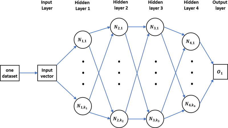
ST-DNN is a regular deep learning algorithm. It only takes care of one single prediction task. Therefore, it only learns from one specific training dataset. A typical four-layer ST-DNN is showed in figure 1, where N_i (i = 1, …, 4), represents the number of neurons in the ith hidden layer.

Figure 1:

An illustration of a typical ST-DNN. Only one task (data set) is trained in this network. Four hidden layers are included, k_i (i = 1, 2, 3, 4) represents the number of neurons in the ith hidden layer and N_i,j is the jth neuron in the ith hidden layer. Here, O₁ is the single output for the task.

II.D. Multitask deep neural network (MT-DNN)

The multitask (MT) learning technique has achieved much success in qualitative Merck and Tox21 prediction challenges^48–51. In the MT framework, multiple tasks share the same hidden layers. However, the output layer is attached to different tasks. This framework enables the neural network to learn all the data simultaneously for different tasks. Thus, the commonalities and differences among various datasets can be exploited. It has been showed that MT learning typically can improve the prediction accuracy of relatively small datasets if it combines with relatively larger datasets in its training.

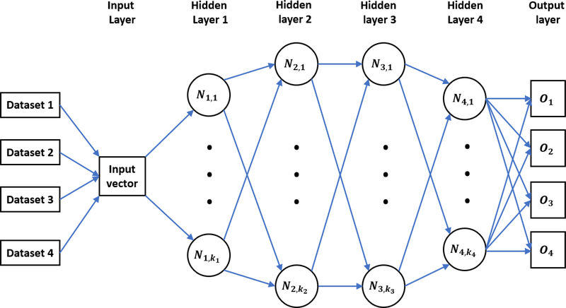
Figure 2 is an illustration of a typical four-layer MT-DNN for training four different tasks simultaneously. Suppose there are totally T tasks and the training data for the tth task are ${\left(X_i^t,y_i^t\right)}_{i=1}^{N_t}$, where t = 1,…,T, i = 1,…,N_t, N_t is the number of samples in the tth task, and $X_i^t$ is the feature vector for the ith sample in the tth task, $y_i^t$ is the label value of the ith sample in the tth task, respectively. The purpose of MT learning is to simultaneously minimize the loss function:

$$\mathrm{argmin}{\sum }_{t=1}^T{\sum }_{i=1}^{N_t}L\left(y_i^t,f^t\left(X_i^t,{\theta }^t\right)\right)$$

where f^t is the prediction for the ith sample in the tth task by our MT-DNN, which is a function of the feature vector $X_i^t$, L is the loss function, and θ^t is the collection of machine learning hyperparameters. A popular cost function for regression is the mean squared error, which can be defined as:

$$L\left(y_i^t,f^t\left(X_i^t,{\theta }^t\right)\right)=\frac{1}{N_t}{\sum }_{i=1}^{N_t}{\left(y_i^t-f^t\left(X_i^t,{\theta }^t\right)\right)}^2.$$

Figure 2:

An illustration of a typical MT-DNN training four tasks (datasets) simultaneously. Four hidden layers are included in this network, k_i (i = 1, 2, 3, 4) represents the number of neurons in the ith hidden layer and N_i,j is the jth neuron in the ith hidden layer. Here O₁ to O₄ represent four predictor outputs for four tasks.

In this study, MT learning technology is applied to the toxicity prediction. The ultimate goal of this MT learning is to potentially improve the overall performance of multiple toxicity prediction models, especially for the smallest dataset that performs relatively poorly in the ST-DNN. More concretely, it is reasonable to assume that different toxicity indexes share a common pattern so that these different tasks can be trained simultaneously when their feature vectors are constructed in the same manner. For our toxicity prediction, four different tasks (LD₅₀, IGC₅₀, LC₅₀, LC₅₀-DM data sets) are trained together. This leads to four output neurons in the output layer (See O₁ to O₄ in Figure 2), with each neuron being specific to one of four tasks.

II.E. Consensus of multiple model predictions

Consensus means the average value from multiple model predictions, which typically enhances the results from individual models.

II.F. Hyperparameters

Ensemble hyperparameters

Both RF and GBDT were implemented by the scikit-learn package (version 0.20.1)⁵². In this work, there are a total of 23 datasets with their training data size varying from 94 to 8199. RF has been showed to be consistent and robust with various datasets. However, if its parameters are carefully tuned based on the size of a given training set, GBDT can attain better performance than RF does in most cases. For all experiments in this work, the most essential parameters of GBDT are chosen as learning rate = 0.01, min_samples_split = 3, max_features=sqrt. Detail values of other parameters are given in Table 2.

Table 2:

RF and GBDT parameters for different training-set sizes.

Training-set size	RF parameters	GBDT parameters
<800	n_estimators=1000, criterion=‘mse’, max_depth=None, min_samples_spNt=2, min_samples_leaf=1, min_weight_fraction_leaf=0.0	n_estimators=2000, max_depth=9, min_samples_split=3, learning_rate=0.01, subsample=0.1, max_features=’sqrt’
800 to 5000		n_estimators=10000, max_depth=7,min_samples_split=3, learning_rate=0.01, subsample=0.3, max_features=’sqrt’
5000 to 10000		n_estimators=20000, max_depth=7,min_samples_split=3, learning_rate=0.01, subsample=0.3, max_features=’sqrt’

Network hyperparameters

Since the numbers of features differ much in different 2D fingerprints, different network architectures have to be adopted. For example, Estate 1 fingerprint has only 79 bits. Therefore a 4-layer network with the number of neurons in various hidden layers are chosen as 500, 1000, 1500, and 500. However, the Daylight fingerprint has as many as 2048 features, and thus a much larger network is needed. The network for this fingerprint still has 4 layers but there are 3000, 2000, 1000, and 500 neurons in the first, second, third and fourth hidden layer, respectively. Other network parameters are as followed: the optimizer is stochastic gradient descent (SGD) with momentum of 0.5. 2000 epochs were run for all the networks. Mini-batch size is set to 4. The learning rate is set to 0.01 in the first 1000 epochs and 0.001 for the rest epochs. Our tests indicate that adding a dropout or using L₂ decay does not necessarily improve the accuracy, and thus, we omit these two techniques. All the network hyperparameters are summarized in Table 3. These hyperparameters are applied to both ST-DNN and MT-DNN. All the DNN training is performed by Pytorch (version 1.0)⁵³.

Table 3:

The network hyperparameters for both ST-DNN and MT-DNN.

Fingerprint	Number of features	Number of hidden layers	Number of neurons in each hidden layer	Optimizer	Mini-batch	Learning rate
Estate1	79	4	500,1000,1500,500	SGD with a momentum of 0.5	4	First 1000: 0.01; Then: 0.001
Estate2	79
Daylight	2048		3000,2000,1000,500

III. Results

III.A. Toxicity prediction

Four toxicity datasets were studied in our work, namely oral rat LD₅₀ (LD₅₀), 40 h Tetrahymena pyriformis IGC₅₀ (IGC₅₀), 96 h fathead minnow LC₅₀ (LC₅₀), and 48 h Daphnia magna LC₅₀ (LC₅₀-DM). Among them, LD₅₀ measures the amount of chemicals that can kill half of rats when orally ingested. IGC₅₀ records the 50% growth inhibitory concentration of Tetrahymena pyriformis organism after 40 h. LC₅₀ reports at the concentration of test chemicals in water in milligrams per liter that cause 50% of fathead minnows to die after 96 h. The last one is LC₅₀-DM, which represents the concentration of test chemicals in water in milligrams per liter that cause 50% Daphnia maga to die after 48 h. The unit of toxicity reported in these four datasets is -log₁₀ mol/L. All of them are accessible from the recent publications^42,54,55 and the public database (https://www.epa.gov/chemicalresearch/toxicity-estimation-software-tool-test). The sizes of these four datasets vary from 353 to 7413 (See Table 4), which raises a challenge for a predictive model to achieve a consistent accuracy and robustness.

Table 4:

The quantitative summary of four toxicity datasets. The original datasets and prediction results are available at https://www.epa.gov/chemical-research/toxicity-estimation-software-tool-test.

Data set	Total size	Train set size	Test set size	Max value	Min value
LD50	7413	5931	1482	7.201	0.291
IGC50	1792	1434	358	6.36	0.334
LC50	823	659	164	9.261	0.037
LC50-DM	353	283	70	10.064	0.117

III.A.1. The performance of ensemble methods

Because it is easy to implement and fast to train, two ensemble methods, RF and GBDT, were first tested. Since four datasets have very different sizes, different numbers of estimators in RF and GBDT models should be used. Specifically, for two relatively small sets, LC₅₀ and LC₅₀-DM, the numbers of estimators are set to 2000. For IGC50, 10000 estimators are used. For the largest set LD₅₀, we have used 20000 estimators.

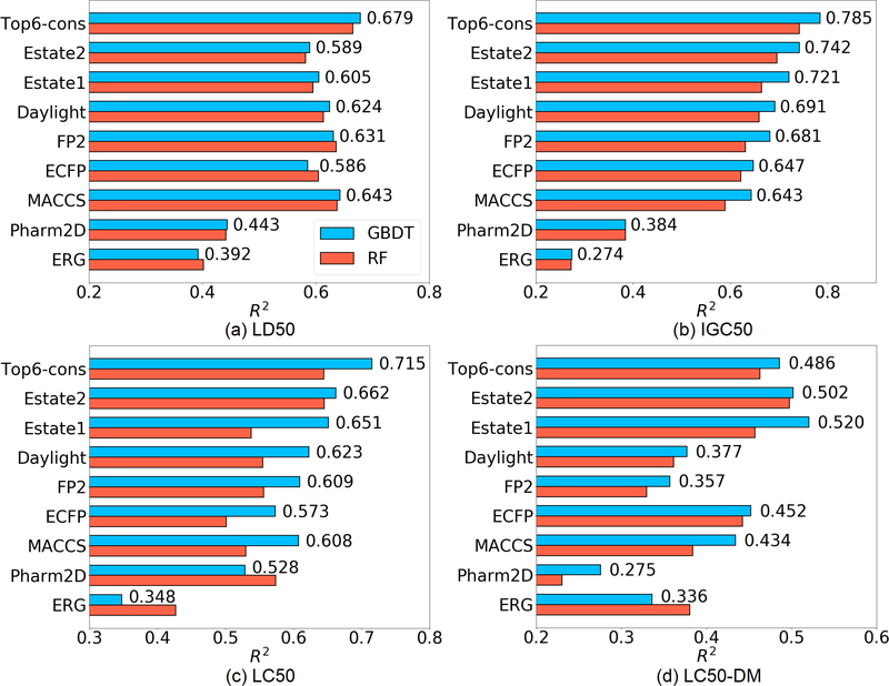
The accuracy is in term of the square of Pearson correlation coefficient (R²). Overall, GBDT’s performance is always better than that of RF, which agrees with early publication⁴. Among all the eight fingerprints we tested, Estate2, Estate1, Daylight, FP2, ECFP and MACCS usually work well on these four sets. Thus the consensus of these six fingerprints or say the average prediction of the six fingerprints, was also considered (“Top 6-cons” in Figure 4). The consensus model typically gives rise to a further improvement over all single fingerprints in most cases.

Figure 4:

The R² on LD₅₀, IGC₅₀, LC₅₀, LC₅₀-DM test sets yielded by eight fingerprints and the consensuses of the top 6 features. Two ensemble methods were adopted (GBDT: blue, RF: red). The values shown in the figure are the R² of GBDT.

(a). LD₅₀ test set

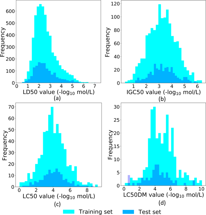
LD₅₀ dataset is the largest set having as many as 7413 compounds. However, thi set has a higher experimental uncertainty of the values (See “Max value” and “Min value” in Table 4) and more importantly, as revealed by Figure 3(a), the ranges of the training set and test set are almost the same. The boundary values of the training set overlap with those of the test set, which brings difficulty for machine learning models. In our GBDT model, the best single fingerprint (MACCS) yields an R² of 0.643, while the consensus of the top 6 fingerprints increases R² to 0.679.

Figure 3:

The sample distributions of LD₅₀, IGC₅₀, LC₅₀, LC₅₀-DM training and test sets.

(b). IGC₅₀ test set

IGC₅₀ set is the second largest set (1792 compounds) among the four sets we investigated. As indicated in Table 4, this set has the smallest range of label. Moreover, Figure 3(b) shows that the test set has a smaller range than that of the training set, indicating a relatively easy case for machine learning models. Our results show that Estate2 is the best single fingerprint with an R² of 0.742, and the consensus of the top 6 fingerprints leads to an R² of 0.785.

(c). LC₅₀ test set

LC₅₀ set is a relative smaller set (823 compounds). Figure 3(c) indicates that the ranges of the training set and test set are almost the same. In our GBDT model, estate2 fingerprint achieves the top performance, which yields an R² of 0.662. The consensus of the top 6 fingerprint improves the R² to 0.715.

(d). LC₅₀-DM test set

Among the four sets, LC₅₀-DM test set is the smallest one with only 283 training molecules and 70 test molecules, which is troublesome to build a robust model. Moreover, revealed by Figure 3(d), not only the boundary values of the training set overlap with those of the test set, but also the test set has a higher distribution at the left boundary, rendering a difficult case for machine learning. Specifically, the best single fingerprint Estate1 only has an R² of 0.520. The consensus model even ruins the R² a little bit with an R² as low as 0.486. Similar difficulty is also faced by other recent work, such as the R² of the 3D-topology based GBDT model only reaches 0.505⁴. Thus, there is a need for multitask deep learning when dealing with such a small dataset.

III.A.2. The performance of single-task and multitask deep learning

On average, Estate2, Estate1, and Daylight are the top three fingerprints when using GBDT models in all the four sets. Thus, these three fingerprints were picked up to perform higher-level ST-DNN and MT-DNN.

Since the lengths of the three fingerprints differ much, different DNN architectures are needed. Four hidden layers with 500, 1000, 1500, and 500 neurons are used for Estate1 and Estate2, whose fingerprints have 79 features. Four hidden layers with 3000, 2000, 1000, and 500 neurons are used for Daylight, whose fingerprint has 2048 bits.

The pattern of ST-DNN results is similar to that of GBDT results. On four data sets, a ST-DNN consensus model yields an average R² of 0.658 (0.632, 0.791, 0.687, and 0.523 respectively). As a comparison, the average R² by a GBDT consensus model is 0.666 (0.679, 0.785, 0.715, and 0.486 respectively). However, the performance can be largely enhanced by the multitask strategy because the two relatively smaller sets LC₅₀ and LC₅₀-DM can benefit much from two larger sets LD₅₀ and IGC₅₀. As shown in Table 5, while the MT-DNN model seldom changes the performance on LD₅₀ and IGC₅₀, it gives rise to a dramatic improvement on LC₅₀ and LC₅₀-DM, especially on LC₅₀-DM. The consensus lifts the R² result from 0.523 to 0.725.

Table 5:

The R² of ST-DNN and MT-DNN based on the top 3 fingerprints in GBDT (Estate2, Estate1, Daylight) and their consensuses.

Method	R2 of LD50	R2 of IGC50	R2 of LC50	R2 of LC50-DM
Estate2 ST-DNN	0.484	0.715	0.569	0.433
Estate2 MT-DNN	0.489	0.696	0.660	0.623
Estate1 ST-DNN	0.569	0.733	0.650	0.601
Estate1 MT-DNN	0.566	0.735	0.694	0.684
Daylight ST-DNN	0.619	0.701	0.570	0.346
Daylight MT-DNN	0.617	0.717	0.724	0.694
Consensus ST-DNN	0.632	0.791	0.687	0.523
Consensus MT-DNN	0.639	0.794	0.765	0.725

III.A.3. Systematic comparison with other toxicity predictions

A systematic comparison with other methods was provided in Table 6. The same datasets are also used to develop the Toxicity Estimation Software Tool (T.E.S.T). So many related results can be found in its user’s guide⁴², including hierarchical, single model, FDA, group contribution, nearest neighbor, and T.E.S.T consensus. Since T.E.S.T is also based on 2D descriptors, the comparison between the results from the present models and T.E.S.T can largely reflect the predictive power of the present models. As shown in Table 6, on the LD₅₀, IGC₅₀, LC₅₀ sets, the present MT-DNN consensus always leads to a higher R² than T.E.S.T consensus. Especially, on the IGC₅₀ and LC₅₀ sets, the present MT-DNN consensus models largely beat T.E.S.T (0.794 vs 0.764 and 0.765 vs 0.728), and the present GBDT results quite outperform T.E.S.T (0.679 vs 0.626) on the LD₅₀ set. Even on the LC50-DM set, because the training set is so small (283), ensemble methods (RF and GBDT) and DNN methods are not suitable for it: R² of ST-DNN and GBDT are, respectively, 0.523 and 0.486. However, the R² of MT-DNN is as high as 0.725 for LC₅₀-DM dataset, which is quite comparable to the T.E.S.T result with an R² of 0.739.

Table 6:

Comparison to other toxicity prediction methods. The prediction results for Hierarchical, Single model, FDA, Group contribution, Nearest neighbor, and T.E.S.T consensus are available in reference 44 and at https://www.epa.gov/chemical-research/toxicity-estimation-software-tool-test.

LD50
Method	R2	RMSE	Coverage
The present 2D MT-DNN consensus	0.639	0.549	1.000
The present 2D GBDT consensus	0.679	0.580	1.000
Hierarchical42	0.578	0.650	0.876
FDA42	0.557	0.657	0.984
Nearest neighbor42	0.557	0.656	0.993
T.E.S.T consensus42	0.626	0.594	0.984
3D MT-DNN consensus4	0.653	0.568	0.997
IGC50
Method	R2	RMSE	Coverage
The present 2D MT-DNN consensus	0.794	0.457	1.000
The present 2D GBDT consensus	0.785	0.457	1.000
Hierarchical42	0.719	0.539	0.933
FDA42	0.747	0.489	0.978
Group contribution42	0.682	0.575	0.955
Nearest neighbor42	0.600	0.638	0.986
T.E.S.T consensus42	0.764	0.475	0.983
3D MT-DNN consensus4	0.802	0.438	1.000
LC50
Method	R2	RMSE	Coverage
The present 2D MT-DNN consensus	0.765	0.718	1.000
The present 2D GBDT consensus	0.715	0.783	1.000
Hierarchical42	0.710	0.801	0.951
Single model42	0.704	0.803	0.945
FDA42	0.626	0.915	0.945
Group contribution42	0.686	0.810	0.872
Nearest neighbor42	0.667	0.876	0.939
T.E.S.T consensus42	0.728	0.768	0.951
3D MT-DNN consensus4	0.789	0.677	1.000
LC50-DM
Method	R2	RMSE	Coverage
The present 2D MT-DNN consensus	0.725	0.935	1.000
The present 2D GBDT consensus	0.486	1.239	1.000
Hierarchical42	0.695	0.979	0.886
Single model42	0.697	0.993	0.871
FDA42	0.565	1.190	0.900
Group contribution42	0.671	0.803	0.657
Nearest neighbor42	0.733	0.975	0.871
T.E.S.T consensus42	0.739	0.911	0.900
3D MT-DNN consensus4	0.678	0.978	1.000

2D MT-DNN consensus has an average R² of 0.731 for these four datasets, while the average of T.E.S.T model is 0.714, and the recent 3D structure-based topological MT-DNN consensus result is also 0.731⁴. These results confirm that 2D fingerprints integrated with MT-DNN model surpass the previous 2D models and are as good as the recent 3D structure-based topological model⁴.

III.B. Aqueous solubility (Log S)

For Log S, following the previous literature^5,56, we test Klopman’s test set⁵⁷ with the original train set. The unit of Log P in these sets is log unit. Since the size of the training set is 1290, 10000 estimators were used in the GBDT model.

In the Log S test, the top 6 fingerprints are MACCS, FP2, Daylight, Estate1, Estate2, and ECFP, which perform much better than the other two fingerprints, Pharm2D and ERG. The consensuses of the top 6 fingerprints results in R and RMSE of 0.944 and 0.684, respectively. The consensus of top 3 is even better, which improves R and RMSE to 0.955 and 0.648 (See Table 8). A systematic comparisons to other methods are included in Table 9. It indicates the present method outperforms all other state-of-the-art 3D and 2D methods.

Table 8:

The R and RMSE of predicting Log S by eight fingerprints and the consensuses of the top 3 and top 6 on Klopman’s test set.

Fingerprint	R	RMSE
Cons-top 3	0.955	0.648
Cons-top 6	0.944	0.684
MACCS	0.958	0.664
Estate1	0.932	0.791
Daylight	0.923	0.780
FP2	0.908	0.853
ECFP	0.904	0.875
Estate2	0.897	0.907
Pharm2D	0.832	1.114
ERG	0.811	1.202

Table 9:

Comparison of prediction results on the Log S data set.

Method	R	RMSE
Cons-top 3	0.955	0.648
Cons-top 6	0.944	0.684
MT-ESTD+-1 (3D)5	0.94	0.69
Drug-LOGS (2D)56	0.94	0.64
Klopman MLR (2D)57	0.92	0.86

III.C. Partition coefficient (Log P)

Three Log P data sets were tested using the GBDT model. The training set has 8199 molecules, which was originally compiled by Cheng et al.⁵⁸. There are three test sets, namely FDA⁵⁸, Star⁵⁹, and Non-star⁵⁹ respectively, which are given in Table 10. The Log P in these sets is by the unit of log₁₀ mol/L. Due to the size of the training set, 20000 estimators are used in the GBDT model.

Table 10:

The sizes of Log P training set and test sets.

Training set	Test set
	FDA	Star	Non-star
8199	406	223	43

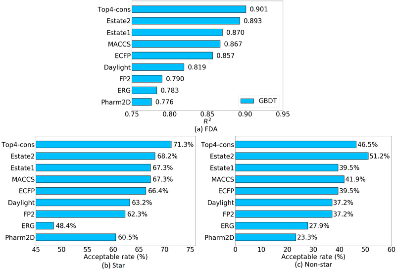
In order to easily compare to the earlier literatures, accuracy on these three test sets are reported by R² or acceptable rate. The acceptable rate here is defined as the percentage of molecules within error range < 0.5⁶⁰. Of all the three sets, the 2D fingerprints of Estate2, Estate1, MACCS, and ECFP are always the top 4. The consensuses of the top 4 fingerprints produce R² up to 0.901 on the FDA set and attain an acceptable rate on Star set at 71.3%. On the Non-star set, the top 4 consensus is somehow worse than the best single fingerprint Estate1 but it is still in the second place with an acceptable rate of 46.5% (See Figure 5).

Figure 5:

The performance of eight fingerprints and the consensuses of the top 4 on the FDA, Star and Non-star data sets of Log P. To be consistent with previous results, on the FDA set, R² is given, while on star and non-star datasets, acceptable rate is given.

A detailed comparison with other Log P prediction methods was shown in Table 11. On the FDA data set, GBDT-ESTD⁺−2-AD⁵ and MT-ESTD-1⁵ are based on 3D descriptors. GBDT-ESTD⁺−2-AD model includes some molecules from the NIH-dataset in its training set. Therefore, its performance is slightly better than the present one. The 2D method ALOGPS⁵⁸ also performs slightly better (0.908 vs 0.901) than the present one. However, a previous study⁵⁶ has pointed out that for the PHYSPROP database⁶¹, the training set of ALOGPS actually contains all of the compounds in the FDA set. It is unclear how well it will perform if the overlapping compounds are removed from the training set. Unlike ALOGPS, XLOGP3’s training data is completely independent of the test set⁵⁸. In this case, the present prediction is more accurate than that of XLOGP3 (0.901 vs 0.872).

Table 11:

Comparison of Log P predictions on the FDA set.

Method	R2	RMSE
GBDT-ESTD+-2-AD (2D+3D)5	0.935	0.51
MT-ESTD-1 (3D)5	0.920	0.57
ALOGPS (2D but the training set contains test set)58	0.908	0.60
Our Cons-top 4 (2D)	0.901	0.63
XLOGP3 (2D)58	0.872	0.72
XLOGP3-AA (2D)58	0.847	0.80
CLOGP (2D)58	0.838	0.88
TOPKAT (2D)58	0.815	0.88
ALOGP98 (2D)58	0.80	0.90
KowWIN (2D)58	0.771	1.10
HINT (2D)58	0.491	1.93

The present results on the Star and Non-star sets are also systematically compared with other stat-of-the-art models as shown in Table 12. For the Star set, we achieve 71% of total number of molecules having the predicted error less than 0.5 (acceptable rate 71%). This result is quite satisfactory and is comparable to the 3D structure-based model developed by Wu et al.⁵ with an acceptable rate of 72% on the same training set (“MT-ESTD-1” in Table 12). There are many commercial software packages developed to predict Log P such as AB/Log P⁶⁰, S/Log P⁶⁰, ACD/log P⁶⁰, etc. However, we cannot validate whether the training sets used in these software packages overlap with the Star set. It is more meaningful when comparing the present model to XLogP3 software⁶⁰ since its training dataset does not contain any molecules in the test set. Again, the present model outperforms XLogP3 package on the Star set with the acceptable rates being 71% and 60%, respectively. In the Non-star set, all of the published methods perform as accurate as those in the FDA and Star data set, since the structures in the Non-star set are relatively new and complex. Thus, our model also only achieves an acceptable rate of 47%. However, it is still tied for the third place among all predictors. This result is even better than some 3D structure-based models, though RMSE is relatively high due to a few large outliers.

Table 12:

Comparison of Log P predictions of the Star and Nonstar sets.

	Star set (N=223)			Non-star set (N=43)
	% of Molecules within error range			% of Molecules within error range
Method	<0.5	<1	RMSE	<0.5	<1	RMSE
AB/LogP60	84	12	0.41	42	23	1.00
MT-ESTD+-1-AD5	77	16	0.49	49	19	0.98
S+logP60	76	22	0.45	40	35	0.87
ACD/logP60	75	17	0.50	44	32	1.00
CLOGP60	74	20	0.52	47	28	0.91
MT-ESTD-15	72	18	0.55	33	28	1.01
ALOGPS60	71	23	0.53	42	30	0.82
Our cons-top 4	71	18	0.625	47	16	1.233
MiLogP60	69	22	0.57	49	30	0.86
KowWIN60	68	21	0.64	40	30	1.05
TLOGP60	67	16	0.74	30	37	1.12
CSLogP60	66	22	0.65	58	19	0.93
SLIPPER-200260	62	22	0.80	35	23	1.23
XLOGP360	60	30	0.62	47	23	0.89
XLOGP260	57	22	0.87	35	23	1.16
QLOGP60	48	26	0.96	21	26	1.42
VEGA60	47	27	1.04	28	30	1.24
SPARC60	45	22	1.36	28	21	1.70
LSER60	44	26	1.07	35	16	1.26
CLIP60	41	25	1.05	33	9	1.54
MLOGP(Sim+)60	38	30	1.26	26	28	1.56
HINTLOGP60	34	22	1.80	30	5	2.72
NC+NHET60	29	26	1.35	19	16	1.71

III.D. Protein-ligand binding affinity prediction

III.D.1. The S1322 dataset

To assess the predictive power of 2D-fingerprint based models, two protein-ligand binding affinity datasets were investigated. The first one is denoted as the S1322 set. It is a high quality data set with 1322 protein-ligand complexes involving 7 protein clusters (labeled as CL1, CL2, ···, CL7)^29,47. It is a subset of the refined set of PDBbind v2015⁶². The other dataset is PDBbind v2016⁶³, in which the refined set excluding the core set in PDBbind v2016 is used as a training data. The core set is a test set. These two sets are summarized in Table 13.

Table 13:

The quantitative summary of the S1322 and PDBbind v2016 data sets.

S1322 set							PDBBind v2016 refined set
CL1	CL2	CL3	CL4	CL5	CL6	CL7	refined set	training set	core set (test set)
333	264	219	156	134	122	94	4057	3767	290

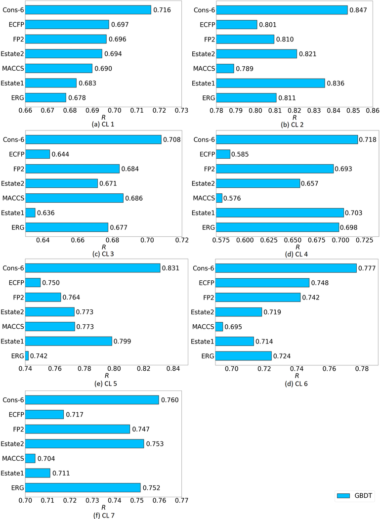
The ligand-based model is used in the present work. For the S1322 set, a 5-fold cross validation was conducted with the GBDT method. To be consistent with the results in the previous literature, accuracy is in term of Pearson correlation coefficient (R). Because the results from Daylight and Pharm2D fingerprints are relatively poor, their results are omitted here. The performance of the other six fingerprints (ECFP, FP2, Estate2, MACCS, Estate1, ERG) and their consensus are shown in Figure 6.

Figure 6:

Pearson correlation coefficient (R) on the seven clusters of the S1322 data set yielded by the six fingerprints (ECFP, FP2, Estate 2, MACCS, Estate 1, ERG) and their consensuses.

Figure 6 indicates that for all the seven clusters, the consensuses of the six fingerprints largely achieve better performance than that of any single fingerprint. Specifically, the R values of consensus models are 0.717, 0.847, 0.708, 0.718, 0.831, 0.777, and 0.760 on each of 7 clusters, respectively and 0.765 on average. These results are comparable to ones achieved by a ligand-based 3D topology and GBDT model²⁸.

III.D.2. PDBbind v2016 refined set and core set

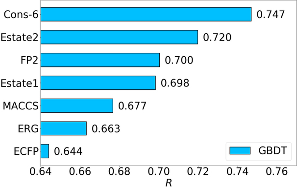
The present ligand-based model was also tested on PDBbind v2016. Rather than cross validation, this time the core set is regarded as a test set. Quite consistent with core validation on the S1322 set, the consensus of the six fingerprints leads to a large improvement than any single one, with an R of 0.747. These results indicate that the present model has a stable and reliable performance on different protein-ligand binding affinity data sets.

For protein-ligand binding affinity prediction, the present 2D fingerprint-based model is not competitive, because protein-ligand binding not only depends on the ligand, but also on the protein. Therefore, for a more accurate prediction, the information of the protein, at least the information of the binding site should be included. State differently, a complex based model is recommended. Recently, Wojcikowski et. al.⁶⁴ reports 2D fingerprint-based complex models. In their work, a recently developed 2D fingerprint model is used to encode protein-ligand complex information. When combined with DNN, their method gives rise to an R of 0.817 on the PDBBind v2016 core set. Table 14 lists these results.

Table 14:

Comparison of protein-ligand binding affinity predictions PDBbind v2016 core set.

Method	R	RMSE (kcal/mol)
TopBP (Complex)29	0.861	1.65
PLEC FP (Complex)64	0.817	1.71
Our cons-top 6 (Ligand)	0.747	2.02

IV. Discussion

IV.A. General analysis

In the present work, the predictive power of eight popular 2D fingerprints as well as their consensuses on four important drug-related properties (i.e., toxicity, Log S, Log P, binding affinity) was investigated. The present study reveals that with a proper machine learning algorithm, the 2D fingerprint-based models including their consensuses outperform other 2D QSPR approaches in the most cases, especially on the toxicity predictions. Additionally, 2D fingerprint-based models are comparable to state-of-the-art 3D structure-based models in most drug-related property predictions, except for protein-ligand binding affinity prediction. Considering 2D fingerprints are very “cheap” molecular descriptors that are easy and fast to generate, our results are very impressive. It means that 2D fingerprints with appropriate machine learning algorithms are still very valuable for practical problems, such as the prediction of toxicity, the aqueous solubility (Log S), and the partition coefficient (Log P). However, for protein-ligand binding affinity prediction, complex-based models using 3D topological fingerprints have a major advantage over the present 2D fingerprints, i.e., a GBDT model based on 3D topological fingerprints can achieve about 15% more accurate²⁸.

IV.B. The performance analysis of 2D fingerprints

IV.B.1. Analysis of 2D fingerprints for PDBbind v2016 core set predictions

The performance of each 2D fingerprint can be systematically analyzed by comparing the difference between prediction errors of every pair of fingerprints as follows.

1. The relative absolute error for the fth fingerprint on the ith sample (molecule) in the test set is defined by

   $${\mathrm{Error}}_{f,i}=\frac{|{\text{prediction}\text{value}}_{f,i}-{\text{experimental}\text{value}}_i|}{|{\text{experimental}\text{value}}_i|}$$

2. For each molecule, the error difference between each pair of fingerprints is calculated.

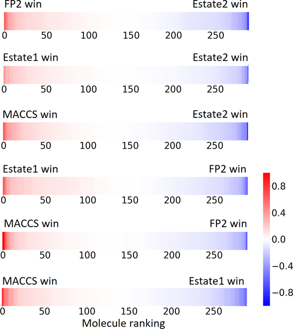
3. Then, the differences for all molecules are ranked from the largest to smallest. The result for PDBbind v2016 core set of 290 complexes is plotted in Figure 8. We have shown all of 6 pairs for the top four 2D fingerprints.

4. To further analyze the strength of each fingerprint on certain molecules, we collect those molecules on which a fingerprint is able to outperform another fingerprint by 0.4 in the error difference.

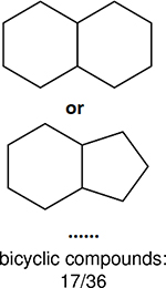
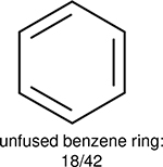
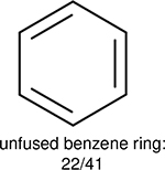
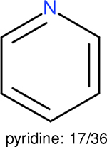
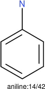
5. Among these molecules for each fingerprint, we identify the top 10 most frequently occurring functional groups. The frequency of the occurrence of each functional group, along with the total of number of molecules, are given in Table 15.

Figure 8:

The ranked error differences between pairs of fingerprints for PDBbind v2016 core set of 290 molecules. Only the top 4 fingerprints (i.e., Estate2, FP2, Estate1, MACCS) are considered.

Table 15:

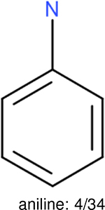
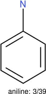
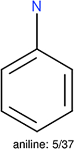
The top 10 frequently occurred functional groups in PDBbind v2016 core set for each fingerprint. For each fingerprint, the occurrence frequency and the total number of molecules are also given.

Ranking	FP2	Estate1	Estate2	MACCS
1
2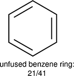
3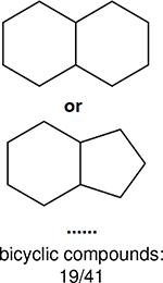
4
5
6
7
8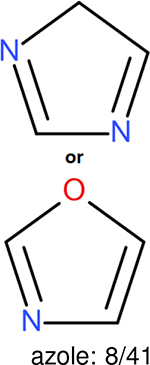
9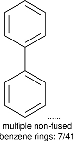
10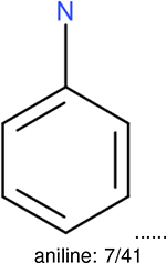

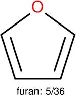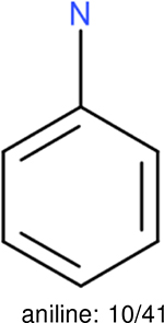
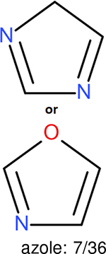
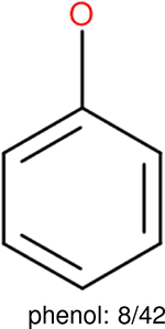
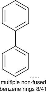
This analysis is quite significant as shown in Table 15. It indicates that different fingerprints have different performance on certain functional groups: some fingerprints perform better on some functional groups, while other fingerprints perform better on other functional groups. Our explanation to this is, the different fingerprints are based on different chemical properties, since different functional groups have different chemical properties, different fingerprints are sensitive to different functional groups. One can find, in the columns for different fingerprints, the number of functional groups are different, this is because, in the table those molecules on which a fingerprint is able to outperform another fingerprint by 0.4 in the error difference are collected, for different fingerprints, the number of such molecules are different.

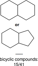
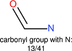
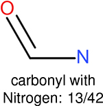
One can select an appropriate fingerprint to represent a certain class of functional groups based on Table 15. For the FP2, Estate1, and Estate2 fingerprints, the top two functional groups are carbonyl groups and unfused benzene rings. However, the MACCS fingerprint is different. Its top two functional groups are bicyclic compounds and pyridine. The third top functional groups differ much for four fingerprints: bicyclic compounds for FP2, aniline for Estate1, carboxylate ion for Estate2, and ether for MACCS, which gives us more information to choose fingerprints. Such as, if one has a molecule including aniline, then Estate1 should be selected. Noticeably, some functional groups occur exclusively for one or two types of fingerprints. For example, F, Cl, Br, I is only on the lists of FP2 and Estate1. While azole appears only on the list of FP2 and MACCS and multiple non-fused benzene rings are only for FP2 and Estate 2. Moreover, phenol occurs only for Estate1 and furan occurs only for MACCS.

IV.B.2. Analysis of 2D fingerprints for the IGC₅₀ toxicity data set prediction and also other data sets

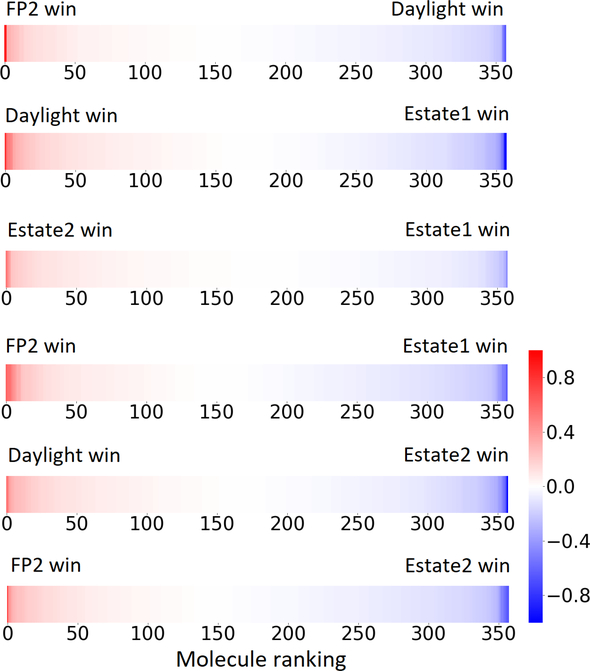
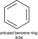
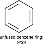
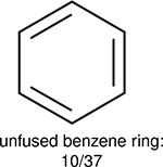
Using the same 5-step procedure outlined above, we carry out a performance analysis for toxicity dataset IGC₅₀, which is shown in Figure 9 and Table 16. The molecules in the toxicity data set are typically small and simple, leading to the functional groups in Table 16 also small. Moreover, since there are not too many functional groups in these relatively simple molecules, only top 8 functional groups are presented in the table. Similar to the performance on the binding affinity, for the top 4 fingerprints on the toxicity set, the carbonyl group is in the first place. Unfused benzene rings also have a high occurrence frequency, resulting in the second or third ranking. The difference between the performance of various fingerprints is mainly located on sulfide and aliphatic chains with 8 or more members. FP2 fingerprint works well on sulfide, whereas, Daylight, Estate1 and Estate2 work well on aliphatic chains with 8 or more members.

Figure 9:

The ranked error differences between pairs of fingerprints for IGC₅₀ toxicity set of 358 molecules. Only the top 4 fingerprints (i.e., Estate2, FP2, Estate1, Daylight) are considered.

Table 16:

The top 10 frequently occurred functional groups in IGC₅₀ toxicity set for each fingerprint. For each fingerprint, the occurrence frequency and the total number of molecules are also given.

Ranking	FP2	Daylight	Estate1	Estate2
1
2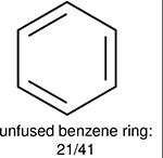
3
4
5
6
7		aliphatic chains with 8 or more members: 5/34	aliphatic chains with 8 or more members: 6/39	aliphatic chains with 8 or more members: 5/37
8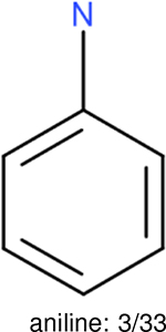

The same performance analyses were also conducted for other toxicity and log P data sets, the results are shown in Tables S1 to S4. These tables indicate, for the toxicity data sets of LD₅₀, LC₅₀, LC₅₀-DM, the performance of the Estate1 and Estate2 fingerprints are similar, they both work well on bicycle compounds; comparing to it, the FP2 fingerprint works better on aliphatic chains with 8 or more members, the daylight fingerprint has a better performance on amide. For log P data set, the ECFP and Estate2 fingerprints lead to a good performance on aniline, the Estate 1 fingerprints works better on bicycle compounds; MACCS fingerprint works better on unfused benzene ring.

IV.C. The predictive power of the consensus of 2D fingerprints

The consensus of several different fingerprints typically further enhances the performance of a single fingerprint. This enhancement can be quite significant. However, on the datasets of different drug-related properties, the best fingerprint combinations for the consensus are not consistent. One possible explanation is that different fingerprints are good at encoding certain functional groups, and datasets for different drug-related properties have different functional group distributions. This is also the reason why a consensus can enhance performance. The consensus can capture more functional groups and counter-balance the systematical bias from different fingerprints.

On toxicity prediction, the best combination for consensus is obtained with Estate2, Estate1, Daylight, FP2, ECFP, and MACCS. On the Log S prediction, the best combination is achieved with MACCS, Estate1, and Daylight. While on the Log P prediction, the best consensus involves Estate2, Estate1, ECFP, and MACCS. Finally, on the binding affinity prediction, the best consensus uses Estate2, Estate1, FP2, ECFP, MACCS, and ERG. It is worth noting that, Estate related (Estate1, Estate2 or both) models are always included in the best combinations. In fact, their single performances are relatively good. This finding is not surprising since Estate fingerprints encode the intrinsic electronic state of the atom as perturbed by the electronic influence of all other atoms. It is well-known that electronic state is important to drug-related properties.

IV.D. Multitask deep learning

Multitask deep learning was utilized on our toxicity prediction. It turns out that the smallest set LC₅₀-DM with only 283 training samples benefits dramatically from the multitask deep learning strategy. Its R² value rises from 0.523 to 0.725. This is because, in the frame of multitask deep learning, different data sets (tasks) share similar structure-function relationships. When a small dataset is trained with a large dataset through shared neural networks, the statistics learned from the large datasets in the shared neurons can help predict the small dataset property. As a result, the other three large toxicity sets can share their patterns learned from training with the small toxicity set, enhancing its prediction. Therefore, multitask deep learning could be a useful strategy to train relatively small datasets.

IV.E. The limitation and advantage of 2D fingerprints

Typically, 2D fingerprints only encode small molecules, such as ligands, although high level 2D fingerprint models including both proteins and ligands have also been developed^64,65. Theoretically, 2D fingerprints are more suitable for target-independent or target-unspecific problems involving small molecules, such as toxicity, solvation free energy, aqueous solubility, partition coefficient, permeability, etc. The current investigation confirms this point. For toxicity, aqueous solubility and partition coefficient, the present 2D-fingerprint based methods perform quite similar to or even somewhat better than 3D structure-based methods in some cases.

For protein-ligand binding affinity predictions, both ligand-based approaches and complex-based are examined. For ligand-based approaches, 2D-fingerprint based methods can perform as well as 3D structure-based models. However, 3D structure-based topological models²⁹ outperform 2D-fingerprint based methods (i.e., R: 0.861 vs 0.747 for PDBbind v2016 core test). In fact, more sophisticated 2D fingerprint models that utilize the protein-ligand complex information and DNN^64,65 are still not as accurate as 3D topology-based models²⁹(i.e., R: 0.817 vs 0.861 for PDBbind v2016 core test and 0.774 vs 0.808 for PDBbind v2013 core test). Essentially, algebraic topology is designed to simplify the geometric complexity of biological macromolecules. Therefore, it is able to extract vital information from protein-ligand complexes to predict their binding affinities.

When there is no available 3D experimental structure, 3D models can still largely outperform 2D models on the binding affinity prediction. An example occurs in D3R Grand Challenges (D3R GC)⁶⁶, in which binding affinities are to be predicted without given 3D experimental structures. Therefore, 3D models can only be built from docking. Even in this circumstance, from GC1 to recent GC4^41,66–68, 3D models has been always proven to be more reliable than 2D models. For example, in recent GC4⁶⁶, our 3D model (receipt ID ar5p6) achieved the smallest RMSE_c at 0.47 kcal/mol, while the best 2D model in that competition attained RMSE_c as high as 0.53 kcal/mol. These results confirm the 3D structured-based model is superior to 2D counterpart in binding affinity prediction even there is no crystal structure.

Moreover, binding affinities typically depend on target (protein). The same ligand can have quite different binding affinities on different targets. The 3D models can take care of binding affinities on different targets but for most 2D models, because of lacking protein information, they work only for a single target.

In general, 2D models can only take care of simple geometry and do not work as well as 3D models do for macromolecules that have complex 3D structures⁴³. The complexity of biomolecular structure, function, and dynamics often makes 2D models inconclusive, inadequate, inefficient and sometimes intractable. In contrast, 3D models can easily handle the complexity of biomolecular structures.

However, the advantage of 2D fingerprints is, they are much easier to generate than 3D structure-based fingerprints built from algebraic topology, differential geometry or various graph theory. Therefore, 2D-fingerprint based models can be useful tools for preliminary drug screening studies.

V. Conclusion

Two-dimensional molecular fingerprints, or 2D fingerprints, refer to molecular structural patterns, such as elemental composition, atomic connectivity, functional groups, 2D-pharmacophores etc. extracted from a molecule without taking into account the 3D-structural representation of these properties. 2D fingerprints have been a main workhorse for cheminformatics and bioformatics for decades. However, their validations in various datasets were typically carried out long time ago with earlier machine learning algorithms. Recently, new 3D structure-based molecular fingerprints built from algebraic topology^28,29, differential geometry³⁰, geometric graph theory^31,32, and algebraic graph theory³³ have found much success in drug discovery related applications^4,5,28,29, including D3R Grand Challenges^33,41. It raises an interesting issue whether 2D fingerprints are still competitive in drug discovery related applications.

This work reassesses 2D fingerprints for their performance in drug discovery related applications. We consider a total of eight commonly used 2D fingerprints, namely FP2, Daylight, MACCS, Estate1, Estate2, ECFP, Pharm2D, and ERG. Four types of drug discovery related applications with 23 datasets, including solubility (Log S) and partition coefficient (Log P) that are independent of a target protein, toxicity that may depend on certain unknown target proteins, and protein-ligand binding affinity that depend on known target proteins, are designed to validate 2D fingerprints. Advanced machine learning algorithms, including random forest (RF), gradient boosting decision trees (GBDT), single-task deep neural network (ST-DNN), and multitask deep neural network (MT-DNN) are used to optimize the performance of the above 2D fingerprints in the aforementioned four types of datasets. In particular, MT-DNN is designed to enhance the performance of 2D fingerprints on relatively small datasets by a simultaneous training with relatively large datasets that share a similar pattern. Since each fingerprint may have an explicit bias on certain functional groups or 2D patterns, we carry out various consensus to further boost the performance of 2D fingerprints in all the datasets. Finally, the strengths of top four 2D fingerprints for predicting protein-ligand binding affinity and quantitative toxicity are analyzed in detail.

Our general findings are as follows. 1) 2D fingerprint-based models are as good as 3D structure-based models for various toxicity, Log S and Log P datasets under the same training-test condition. 2) For ligand-based protein-ligand binding affinity predictions, 2D fingerprint-based models perform equally well as 3D structure-based models that are based only on ligand 3D structures. 3) 3D structure-based models that utilize 3D protein-ligand complex information outperform 2D fingerprints that based on either ligand information or protein-ligand complex information. 4) Advanced machine learning algorithms, such as DNN and MT-DNN, are crucial for 2D fingerprints to achieve optimal performance. However, Estate related (Estate1, Estate2 or both) models always perform well. 5) There is no 2D fingerprint that outperforms all other 2D fingerprints in all applications. 6) Appropriate consensus of a few 2D models typically achieves better performance. Therefore, if combined with advanced machine learning algorithms, the 2D fingerprints are still competitive in most drug discovery related applications except for those that involve macromolecular structures.

Figure 7:

The R on the PDBbind v2016 binding affinity set yielded by the six fingerprints (ECFP, FP2, Estate 2, MACCS, Estate 1, ERG) and their consensus.

Table 7:

The sizes of Log S training set and Klopman’s test set.

Training set	Klopman’s test set
1290	21

References

- [1].Di L and Kerns EH, Drug-like properties: concepts, structure design and methods from ADME to toxicity optimization, Academic press, 2015. [Google Scholar]
- [2].Henriksen NM, Fenley AT and Gilson MK, Journal of chemical theory and computation, 2015, 11, 4377–4394. [DOI] [PMC free article] [PubMed] [Google Scholar]
- [3].Gao K, Yin J, Henriksen NM, Fenley AT and Gilson MK, Journal of chemical theory and computation, 2015, 11, 4555–4564. [DOI] [PMC free article] [PubMed] [Google Scholar]
- [4].Wu K and Wei G-W, Journal of chemical information and modeling, 2018, 58, 520–531. [DOI] [PubMed] [Google Scholar]
- [5].Wu K, Zhao Z, Wang R and Wei G-W, Journal of computational chemistry, 2018, 39, 1444–1454. [DOI] [PubMed] [Google Scholar]
- [6].Lipinski CA, Lombardo F, Dominy BW and Feeney PJ, Advanced drug delivery reviews, 1997, 23, 3–25. [DOI] [PubMed] [Google Scholar]
- [7].Di L and Kerns EH, Drug discovery today, 2006, 11, 446–451. [DOI] [PubMed] [Google Scholar]
- [8].Hopkins AL, Keserü GM, Leeson PD, Rees DC and Reynolds CH, Nature reviews Drug discovery, 2014, 13, 105. [DOI] [PubMed] [Google Scholar]
- [9].Atallah P, Wagener KB and Schulz MD, Macromolecules, 2013, 46, 4735–4741. [Google Scholar]
- [10].Van De Waterbeemd H and Gifford E, Nature reviews Drug discovery, 2003, 2, 192. [DOI] [PubMed] [Google Scholar]
- [11].Hansch C, Maloney PP, Fujita T and Muir RM, Nature, 1962, 194, 178. [Google Scholar]
- [12].Geppert H, Vogt M and Bajorath J, Journal of chemical information and modeling, 2010, 50, 205–216. [DOI] [PubMed] [Google Scholar]
- [13].Roy K and Mitra I, Current computer-aided drug design, 2012, 8, 135–158. [DOI] [PubMed] [Google Scholar]
- [14].Tareq Hassan Khan M, Current drug metabolism, 2010, 11, 285–295. [DOI] [PubMed] [Google Scholar]
- [15].Rogers D and Hahn M, Journal of chemical information and modeling, 2010, 50, 742–754. [DOI] [PubMed] [Google Scholar]
- [16].Lo Y-C, Rensi SE, Torng W and Altman RB, Drug discovery today, 2018, 23, 1538–1546. [DOI] [PMC free article] [PubMed] [Google Scholar]
- [17].Cereto-Massagué A, Ojeda MJ, Valls C, Mulero M, Garcia-Vallvé S and Pujadas G, Methods, 2015, 71, 58–63. [DOI] [PubMed] [Google Scholar]
- [18].Verma J, Khedkar VM and Coutinho EC, Current topics in medicinal chemistry, 2010, 10, 95–115. [DOI] [PubMed] [Google Scholar]
- [19].Durant JL, Leland BA, Henry DR and Nourse JG, Journal of chemical information and computer sciences, 2002, 42, 1273–1280. [DOI] [PubMed] [Google Scholar]
- [20].O’Boyle NM, Banck M, James CA, Morley C, Vandermeersch T and Hutchison GR, Journal of cheminformatics, 2011, 3, 33. [DOI] [PMC free article] [PubMed] [Google Scholar]
- [21].I. Daylight Chemical Information Systems, Daylight, https://hadoop.apache.org.
- [22].Hall LH and Kier LB, Journal of Chemical Information and Computer Sciences, 1995, 35, 1039–1045. [Google Scholar]
- [23].McGregor MJ and Muskal SM, Journal of chemical information and computer sciences, 1999, 39, 569–574. [DOI] [PubMed] [Google Scholar]
- [24].Mason JS and Cheney DL, Biocomputing 2000, World Scientific, 1999, pp. 576–587. [DOI] [PubMed] [Google Scholar]
- [25].Stiefl N, Watson IA, Baumann K and Zaliani A, Journal of chemical information and modeling, 2006, 46, 208–220. [DOI] [PubMed] [Google Scholar]
- [26].Duvenaud DK, Maclaurin D, Iparraguirre J, Bombarell R, Hirzel T, Aspuru-Guzik A and Adams RP, Advances in neural information processing systems, 2015, pp. 2224–2232. [Google Scholar]
- [27].Yang K, Swanson K, Jin W, Coley C, Eiden P, Gao H, Guzman-Perez A, Hopper T, Kelley B, Mathea M et al. , arXiv preprint arXiv:190401561, 2019. [Google Scholar]
- [28].Cang Z and Wei G-W, International journal for numerical methods in biomedical engineering, 2018, 34, e2914. [DOI] [PubMed] [Google Scholar]
- [29].Cang Z, Mu L and Wei G-W, PLoS computational biology, 2018, 14, e1005929. [DOI] [PMC free article] [PubMed] [Google Scholar]
- [30].Nguyen DD and Wei G-W, International journal for numerical methods in biomedical engineering, 2019, 35, e3179. [DOI] [PMC free article] [PubMed] [Google Scholar]
- [31].Nguyen DD, Xiao T, Wang M and Wei G-W, Journal of chemical information and modeling, 2017, 57, 1715–1721. [DOI] [PubMed] [Google Scholar]
- [32].Bramer D and Wei G-W, The Journal of chemical physics, 2018, 148, 054103. [DOI] [PubMed] [Google Scholar]
- [33].Nguyen DD, Cang Z, Wu K, Wang M, Cao Y and Wei G-W, Journal of computer-aided molecular design, 2019, 33, 71–82. [DOI] [PMC free article] [PubMed] [Google Scholar]
- [34].Svetnik V, Liaw A, Tong C, Culberson JC, Sheridan RP and Feuston BP, Journal of chemical information and computer sciences, 2003, 43, 1947–1958. [DOI] [PubMed] [Google Scholar]
- [35].Schapire RE, Nonlinear estimation and classification, Springer, 2003, pp. 149–171. [Google Scholar]
- [36].Basheer IA and Hajmeer M, Journal of microbiological methods, 2000, 43, 3–31. [DOI] [PubMed] [Google Scholar]
- [37].Caruana R, Machine learning, 1997, 28, 41–75. [Google Scholar]
- [38].Abadi M, Agarwal A, Barham P, Brevdo E, Chen Z, Citro C, Corrado GS, Davis A, Dean J, Devin M, Ghemawat S, Goodfellow I, Harp A, Irving G, Isard M, Jia Y, Jozefowicz R, Kaiser L, Kudlur M, Levenberg J, Mané D, Monga R, Moore S, Murray D, Olah C, Schuster M, Shlens J, Steiner B, Sutskever I, Talwar K, Tucker P, Vanhoucke V, Vasudevan V, Viégas F, Vinyals O, Warden P, Wattenberg M, Wicke M, Yu Y and Zheng X, TensorFlow: Large-Scale Machine Learning on Heterogeneous Systems, 2015, https://www.tensorflow.org/, Software available from tensorflow.org.
- [39].Paszke A, Gross S, Chintala S, Chanan G, Yang E, DeVito Z, Lin Z, Desmaison A, Antiga L and Lerer A, NIPS Autodiff Workshop, 2017. [Google Scholar]
- [40].Cang Z and Wei G-W, Bioinformatics, 2017, 33, 3549–3557. [DOI] [PubMed] [Google Scholar]
- [41].Gaieb Z, Parks CD, Chiu M, Yang H, Shao C, Walters WP, Lambert MH, Nevins N, Bembenek SD, Ameriks MK et al. , Journal of computer-aided molecular design, 2019, 33, 1–18. [DOI] [PMC free article] [PubMed] [Google Scholar]
- [42].Martin T, UserÃćâĆňâĎćs guide for TEST (version 4.2)(Toxicity Estimation Software Tool): A program to estimate toxicity from molecular structure, 2016. [Google Scholar]
- [43].Nguyen DD, Cang Z and Wei G-W, Physical Chemistry Chemical Physics, 2020, 22, 4343–4367. [DOI] [PMC free article] [PubMed] [Google Scholar]
- [44].Landrum G et al. , RDKit: Open-source cheminformatics, 2006. [Google Scholar]
- [45].Morgan H, Journal of Chemical Documentation, 1965, 5, 107–113. [Google Scholar]
- [46].Wang B, Wang C, Wu K and Wei G-W, Journal of computational chemistry, 2018, 39, 217–233. [DOI] [PubMed] [Google Scholar]
- [47].Wang B, Zhao Z, Nguyen DD and Wei G-W, Theoretical Chemistry Accounts, 2017, 136, 55. [Google Scholar]
- [48].Capuzzi SJ, Politi R, Isayev O, Farag S and Tropsha A, Frontiers in Environmental Science, 2016, 4, 3. [Google Scholar]
- [49].Ramsundar B, Liu B, Wu Z, Verras A, Tudor M, Sheridan RP and Pande V, Journal of chemical information and modeling, 2017, 57, 2068–2076. [DOI] [PubMed] [Google Scholar]
- [50].Wenzel J, Matter H and Schmidt F, Journal of chemical information and modeling, 2019, 59, 1253–1268. [DOI] [PubMed] [Google Scholar]
- [51].Ye Z, Yang Y, Li X, Cao D and Ouyang D, Molecular pharmaceutics, 2018, 16, 533–541. [DOI] [PubMed] [Google Scholar]
- [52].Pedregosa F, Varoquaux G, Gramfort A, Michel V, Thirion B, Grisel O, Blondel M, Prettenhofer P, Weiss R, Dubourg V et al. , Journal of machine learning research, 2011, 12, 2825–2830. [Google Scholar]
- [53].Paszke A, Gross S, Massa F, Lerer A, Bradbury J, Chanan G, Killeen T, Lin Z, Gimelshein N, Antiga L et al. , Advances in Neural Information Processing Systems, 2019, pp. 8024–8035. [Google Scholar]
- [54].Akers KS, Sinks GD and Schultz TW, Environmental toxicology and pharmacology, 1999, 7, 33–39. [DOI] [PubMed] [Google Scholar]
- [55].Zhu H, Tropsha A, Fourches D, Varnek A, Papa E, Gramatica P, Oberg T, Dao P, Cherkasov A and Tetko IV, Journal of chemical information and modeling, 2008, 48, 766–784. [DOI] [PubMed] [Google Scholar]
- [56].Hou T, Xia K, Zhang W and Xu X, Journal of chemical information and computer sciences, 2004, 44, 266–275. [DOI] [PubMed] [Google Scholar]
- [57].Klopman G, Wang S and Balthasar DM, Journal of chemical information and computer sciences, 1992, 32, 474–482. [DOI] [PubMed] [Google Scholar]
- [58].Cheng T, Zhao Y, Li X, Lin F, Xu Y, Zhang X, Li Y, Wang R and Lai L, Journal of chemical information and modeling, 2007, 47, 2140–2148. [DOI] [PubMed] [Google Scholar]
- [59].Avdeef A, Absorption and drug development: solubility, permeability, and charge state, John Wiley & Sons, 2012. [Google Scholar]
- [60].Mannhold R, Poda GI, Ostermann C and Tetko IV, Journal of pharmaceutical sciences, 2009, 98, 861–893. [DOI] [PubMed] [Google Scholar]
- [61].Howard P and Meylan W, Physical/chemical property database (PHYSPROP), 1999. [Google Scholar]
- [62].Liu Z, Li Y, Han L, Li J, Liu J, Zhao Z, Nie W, Liu Y and Wang R, Bioinformatics, 2014, 31, 405–412. [DOI] [PubMed] [Google Scholar]
- [63].Su M, Yang Q, Du Y, Feng G, Liu Z, Li Y and Wang R, Journal of chemical information and modeling, 2018, 59, 895–913. [DOI] [PubMed] [Google Scholar]
- [64].Wójcikowski M, Kukiełka M, Stepniewska-Dziubinska MM and Siedlecki P, Bioinformatics, 2019, 35, 1334–1341. [DOI] [PMC free article] [PubMed] [Google Scholar]
- [65].Kundu I, Paul G and Banerjee R, RSC Advances, 2018, 8, 12127–12137. [DOI] [PMC free article] [PubMed] [Google Scholar]
- [66].Parks CD, Gaieb Z, Chiu M, Yang H, Shao C, Walters WP, Jansen JM, McGaughey G, Lewis RA, Bembenek SD et al. , Journal of Computer-Aided Molecular Design, 2020, 34, 99–119. [DOI] [PMC free article] [PubMed] [Google Scholar]
- [67].Gathiaka S, Liu S, Chiu M, Yang H, Stuckey JA, Kang YN, Delproposto J, Kubish G, Dunbar JB, Carlson HA et al. , Journal of computer-aided molecular design, 2016, 30, 651–668. [DOI] [PMC free article] [PubMed] [Google Scholar]
- [68].Gaieb Z, Liu S, Gathiaka S, Chiu M, Yang H, Shao C, Feher VA, Walters WP, Kuhn B, Rudolph MG et al. , Journal of computer-aided molecular design, 2018, 32, 1–20. [DOI] [PMC free article] [PubMed] [Google Scholar]
Associated Data
This section collects any data citations, data availability statements, or supplementary materials included in this article.