

Abstract
Target fishing is the process of identifying the protein target of a bioactive small molecule. To do so experimentally requires a significant investment of time and resources, which can be expedited with a reliable computational target fishing model. The development of computational target fishing models using machine learning has become very popular over the last several years due to the increased availability of large amounts of public bioactivity data. Unfortunately, the applicability and performance of such models for natural products has not yet been reported. This is in part due to the relative lack of bioactivity data available for natural products compared to synthetic compounds. Moreover, the databases commonly used to train such models do not annotate which compounds are natural products, which makes the collection of a benchmarking set difficult. To address this knowledge gap, a dataset comprised of natural product structures and their associated protein targets was generated by cross-referencing 20 publicly available natural product databases with the bioactivity database ChEMBL. This dataset contains 5,589 compound-target pairs for 1,943 unique compounds and 1,023 unique targets. A synthetic dataset comprised of 107,190 compound-target pairs for 88,728 unique compounds and 1,907 unique targets was used to train k-nearest neighbors, random forest, and multi-layer perceptron models. The predictive performance of each model was assessed by stratified 10-fold cross-validation and benchmarking on the newly collected natural product dataset. Strong performance was observed for each model during cross-validation with area under the receiver operating characteristic (AUROC) scores ranging from 0.94 to 0.99 and Boltzmann-enhanced discrimination of receiver operating characteristic (BEDROC) scores from 0.89 to 0.94. When tested on the natural product dataset, performance dramatically decreased with AUROC scores ranging from 0.70 to 0.85 and BEDROC scores from 0.43 to 0.59. However, the implementation of a model stacking approach, which uses logistic regression as a meta-classifier to combine model predictions, dramatically improved the ability to correctly predict the protein targets of natural products and increased the AUROC score to 0.94 and BEDROC score to 0.73. This stacked model was deployed as a web application, called STarFish, and has been made available for use to aid in the target identification of natural products.
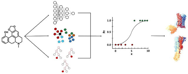
Graphical Abstract
INTRODUCTION:
Experimental approaches for identifying small molecule hits in a drug discovery project typically include target-based screening or phenotypic screening. Target-based approaches involve selecting a protein target believed to be relevant to the disease state of interest and then measuring, directly or indirectly, a compound’s ability to bind the target. Phenotypic approaches are target agnostic and instead measure a compound’s effect on a biologically relevant system, such as cell cytotoxicity or tumor growth inhibition.1 Both approaches are widely used in drug discovery and development. While traditionally viewed as opposing alternatives, target-based and phenotypic assays can also be complementary approaches.2 An important limitation of the phenotypic approach is the inherent lack of understanding of the target and molecular mechanism of action. While a known target and molecular mechanism of action are not required to progress a new chemical entity to the clinic, it is considered a significant risk factor by most large pharmaceutical companies for the clinical development and regulatory approval process.2 Due to the importance of target identification, both experimental and computational target fishing methods have been developed.
The process of experimental target fishing requires a significant investment of time and resources. One method commonly used to directly identify the target protein of a small molecule is biochemical affinity purification. This process involves immobilization of a compound on a column, exposure to cell extracts, stringent washing to remove non-specific binding, proteomic profiling to determine the identity of bound proteins, and ultimately a confirmatory binding assay.3 While this process has been very successful, it is not without limitations.4 For example, it requires the bioactive small molecule to be modified in order to be immobilized on the column. Points of modification can be difficult to determine as they require a synthetic handle in a region where a bulky linker can be attached without interfering with target binding. Overall, experimental target fishing requires a great deal of biological and synthetic expertise and effort.
In an effort to aid and accelerate the target identification process, a variety of computational target fishing methods have been developed. Computational target fishing methods generally fit into one of three broad categories: ligand-based, structure-based, or network-based. A recent review by Sydow et al. gives a good overview on the specifics and current methods applied for each category.5 Ligand-based methods rely on the assumption that proteins will bind similar small molecules. A simple ligand-based target fishing approach typically involves computing Tanimoto similarities between a compound of interest and compounds with known targets in a bioactivity database. The protein targets of compounds with high similarity to a query compound are then predicted as potential protein targets. An early and successful ligand-based target fishing method, similarity ensemble approach (SEA), builds upon this approach by comparing a query molecule’s similarity to a group of compounds of a potential target and assessing the statistical significance of the resulting similarity score.6 The growing amount of publicly available bioactivity data in databases such as ChEMBL and PubChem has made the application of machine learning methods to computational target fishing popular.7,8 Methods such as Random Forest (RF), Support Vector Machines (SVM), and Naive Bayes (NB) have long been used in this regard, but deep learning methods have recently garnered significant attention due to their impressive performance.9-13 The majority of the data that these models were trained with is synthetic compound bioactivity data and despite the impressive performance observed for these machine learning target fishing models, there is little known about how they might perform when applied to natural products.
Natural products have been a tremendous source of new drugs over the past three decades. Unaltered natural products and natural product derivatives comprise over one-third of the FDA approved small molecule drugs.14 Taken even more broadly with the inclusion of “natural product mimics”, natural products account for or have inspired in some way up to 60% of all of these approved drugs. Historically, natural products have made up a substantial portion of first-in-class drugs identified through phenotypic methods.15 Therefore, the process of target identification is very important for natural products, but this area is currently underexplored. An example of applying a computational target fishing model to natural products is the self - organizing map–based prediction of drug equivalence relationships (SPiDER)16, which has been successfully used to identify the targets of several natural products, such as archazolid A.17,18 SPiDER is a ligand-based target-fishing method that was trained and validated on a set of 12,661 compounds and considers 251 biomolecular targets. The prospective use of SPiDER for natural product target identification is encouraging, but its performance was not comprehensively assessed on a dataset of natural products. In 2017, Fang et al. used a network-based target fishing approach for natural product target prediction. A balanced substructure-drug-target network-based inference (bSDTNBI) model was trained and tested on 2,388 unique natural products and 751 targets.19 However, the majority of available binding data is for synthetic compounds and almost all target fishing models are trained using synthetic data. A study by Keum et al. in 2016 developed a target fishing model using the bipartite local model method and support vector machines (SVM) trained on 3,612 compounds and 831 targets.20 The trained model was used to predict the targets of 6,320 natural product compounds. Unfortunately, the protein targets for these natural products were unknown. Model predictions were examined on the basis of whether a predicted target was implicated in the disease state for which a given herb, containing the natural product, was associated. Ultimately, how well a model trained on synthetic data can predict targets for natural products remains unknown.
To address this, a stacked ensemble target fishing (STarFish) approach has been developed and was benchmarked on a newly collected natural product set that considers the largest number of protein targets for a natural product dataset so far. Model stacking is a popular and successful approach in Kaggle competitions and has also been recently applied to other areas of cheminformatics.21-24 This model stacking approach expands upon the idea that the combination of model predictions can produce better predictions than individual models alone. In this study, different combinations of stacked classifiers are trained on a large synthetic data training set comprised of 107,190 compound-target pairs for 88,728 unique compounds and 1,907 unique targets. The trained stacked classifiers are subsequently evaluated through cross-validation on the synthetic compound dataset and through benchmarking on the newly collected natural product dataset comprised of 5,589 compounds-target pairs for 1,943 unique compounds and 1,023 unique targets. Furthermore, a multi-label classification approach is taken. Historically, computational target-fishing models have been trained under the assumption that a single molecule binds a single protein, but in recent years more emphasis has been placed on the consideration of polypharmacology during training.25 Therefore, the individual models which comprise the stacked model are trained on a multi-label classification problem to account for this polypharmacology. Overall, STarFish considers small molecule binding to 1,907 targets and its performance on natural products target prediction is explicitly considered. The datasets, source code, and API are freely available for download and use at: https://github.com/ntcockroft/STarFish.
METHODS:
Dataset
Natural product compound records were extracted from the following freely accessible datasets/databases: AfroCancer26, AfroDb27, AfroMalaria28, AnalytiCon29, Carotenoids30, ConMedNP31, InterBioScreen(IBS) natural product collection32, Mitishamba33, NANPDB34, Natural Product Atlas35, NPACT36, NPASS37, NuBBE38, p-ANAPL39, SANCDB40, Super Natural II41, TCM42, TlPdb43, UNPD44, and ZINC natural product subset45. The compounds from each database were retrieved in various chemical formats and were ultimately converted to simplified molecular-input line-entry system (SMILES) strings if not provided. All of the provided or generated SMILES strings were cleaned and standardized using MolVS.46 The resulting combined set contained 438,258 unique natural products in total. Since the majority of the natural product databases listed do not have bioactivity annotations, the compound set was cross-referenced with the ChEMBL database (version 23) 7 to identify natural product compounds with known protein targets.
The ChEMBL database was queried to retrieve compound activity records which had reported activities (IC50, Ki, Kd, EC50) of 1 μM or better in assays with a confidence score of 9 and had a known target with a corresponding UniProt ID. A confidence score of 9 was selected so that only assay data that resulted in a single protein target being assigned with a high degree of confidence were used. This query yielded a dataset of 485,813 compound-target activity pairs with many redundant activity pairs. The SMILES strings in this dataset were cleaned and the natural product dataset was standardized using MolVS. Following standardization, the ChEMBL dataset was used to determine protein targets for the natural product dataset by identifying InChIKeys or SMILES that were present in both datasets. After this comparison, any redundant compound- target pairs were removed, which yielded two datasets: a “synthetic” set consisting of 395,590 unique compound-target pairs and a natural product set consisting of 6,339 unique compound-target pairs.
The synthetic set was pruned further prior to model training. Only compound-target pairs containing targets with at least 10 compounds were kept. Furthermore, the number of compounds per target class was capped at 100 through random sampling to limit the imbalance between protein target classes. This pruning resulted in 107,190 compound-target pairs for 88,728 unique compounds and 1,907 unique targets. A breakdown of the target protein classes present in these 1,907 unique targets is shown in Figure 1. For the natural product dataset, compound-target pairs that contained protein targets in common with the pruned synthetic set (Figure SI) were retained resulting in 5,589 compound-target pairs for 1,943 unique compounds and 1,023 unique targets. The size of the collected natural product dataset relative to the number of targets considered was insufficient to be used for both model training and validation on its own. Therefore, the synthetic set was used for model training and cross-validation while the natural product set was used to benchmark model performance on a more realistic and difficult test case.
Figure 1.

Sankey diagram of the protein classes present in the ChEMBL23 activity data used in model training. The proportion of protein targets belonging to L1 and L2 protein classes as defined by ChEMBL is represented by line thickness.
All compound-target activity pairs were converted to a multi-label format. For each compound record, a binary label vector was constructed that annotated the protein targets to which these compounds are known to bind. On average, compounds in the synthetic compound dataset have 1.2 annotated protein targets per compound and compounds in the natural product dataset have 2.9 annotated protein targets per compound. Therefore, while 1,907 possible target associations are considered for each compound, these associations have not all been tested experimentally and most are unknown. It was assumed that for these unknown cases that the compound did not bind to the protein and this unknown data was treated as negative data. According to a recent estimate of drug polypharmacology, drugs have on average 11.5 targets below 10 μM.47 Applying this estimate to the unknown small molecule compound-target associations implies a negative label would be correct for 99% of the labels. However, it is likely that many compound records will be assigned a negative protein target label for a protein that they actually interact with. This will influence training as strong classifier predictions for such labels would be penalized. Additionally, during performance evaluation such labels are considered false positives and negatively impact performance when ranked highly. While the assumption of negative labels for unknown compound-protein target records is reasonable, there are indeed drawbacks.
The use of a multi-label format does not fully capture the ways in which compounds can interact with protein targets. While a set of ligands may all be reported to bind to a common protein, the compounds may bind at different sites or have different effects on the protein. For example, one compound may bind to a catalytic site on the protein while another binds to an allosteric site. Additionally, two compounds may bind to the same site on the protein, but one may be an agonist while the other an antagonist. Currently, there is not sufficient data regarding these potential binding differences for the 1,907 targets considered and so in the multi-label format described here, these pharmacological differences are ignored and all compound-protein interactions are treated as equivalent. Therefore, a classifier trained using ligands that bind to the catalytic site would be expected to perform poorly when used to predict the target of compounds which bind to the allosteric site of the same protein.
Compound Descriptors
RDKit was used to generate molecular fingerprints for each compound.48 Molecular fingerprints are bit vector representations of a compound. A kernel is applied to a molecule to extract chemical features, hash them, and set bits based on the hash. If two compounds contain the same functional group they will both set a bit for that functional group. However, more than one functional group can set the same bit resulting in collisions. Increasing the number of bits used to represent molecules reduces collisions, but increases the computational cost of working with the fingerprint. The SMILES string for each compound was converted to a 2048 bit Morgan Functional-Class Fingerprint (FCFP) using a radius of 2. FCFP was selected over Extended-connectivity fingerprints (ECFP) to generate a more abstract and pharmacophoric representation of each compound.49
Machine Learning Models
All models were built using Scikit-Learn 0.19.1 in Python 3.6.5.50 Since compounds can bind to more than one target protein, compound-target identification was formulated as a multi-label classification problem. Different classification models handle multi-label classification problems differently and therefore how each handles multi-label problems is addressed specifically for each classifier. Additionally, each classifier was asked to predict label probabilities instead of assigning labels directly.
k-Nearest Neighbors
The k-nearest neighbors (KNN) algorithm is a type of instance-based learning and computes the distance between the query point and the training instances to determine the closest k points. The KNN classification scheme is easily applied to a multi-label format. In a multi-label case, the query point is assigned the class labels of the closest k points with the probability of each label corresponding to the simple average of label counts over k points. These probabilities can also be weighted by the distance of each training instance to the query point. The KNN model used herein was trained using 10 neighbors, brute force distance calculations with the Jaccard metric, and uniform weights.
Multi-layer Perceptron
A multi-layer perceptron (MLP) is class of feedforward artificial neural networks that consists of at least three layers: an input layer, a hidden layer, and an output layer. Each layer consists of a set of neurons. In the input layer, the number of neurons is set to the number of features for a record in the training data. In the case of the 2048 bit Morgan fingerprint, the number of neurons in the input layer is 2048; one neuron for each bit. When used for classification, the number of neurons in the output layer corresponds to the number of class labels, in this case one neuron per protein target, and is inherently applicable to multi-label problems. The MLP classifier used herein consists of a single hidden layer with 1000 neurons and ReLU activation function. A stochastic gradient-based optimizer referred to as “Adam” was the solver used for weight optimization with an initial learning rate of 0.001, an exponential decay rate of 0.9 and 0.999 for the first and second moment vectors respectively, and the constant for numerical stability set to 1e-8. The maximum number of iterations was set to 200 with a convergence tolerance of 1e-4 after 2 consecutive iterations.
Random Forest
Random forests are an ensemble of decision trees that can be used for either classification or regression. While inherently applicable to multi-label problems, there are technical limitations, such as memory consumption, when training with a large amount of high-dimensional data and trying to predict a large number of class labels. To circumvent this issue, the multi-label problem was re-cast as many individual binary classification problems. In the multi-label learning literature, this strategy is referred to as one-vs-the-rest or binary relevance. Therefore, a random forest model was trained for each label and to predict whether that label should be assigned or not. A total of 1,907 random forest models were trained, one for each protein target, using 1,000 trees and 45 features were considered when looking for the best split.
Logistic Regression
Despite the name, logistic regression is used for classification and can be applied to binary, multinomial, and ordinal classification problems. Logistic regression is a linear method, however, the output of the linear combination of features is bounded between 0 and 1 by using a logistic function. To apply logistic regression to a multi-label classification problem, the one-vs-the-rest strategy described above must also be applied here. Logistic regression models were trained using the “liblinear” solver and L2 regularization. A total of 1,907 logistic regression models were trained, one for each protein target, with C=1.0.
Model Stacking
Model stacking, also referred to as stacked generalization or meta ensembling, is a method which combines information from base models to generate a new model. A stacking approach takes advantage of the fact that individual models may have different strengths in label prediction compared to others and attempts to improve prediction through their combination. During stacking, the input features, in this case the level 0 data, is passed to all individual base models, the level 0 classifiers, which yield predicted probabilities for each individual label. These predicted label probabilities, the level 1 data, are then used as the input features for the next model, the level 1 classifiers. Although this process can continually be repeated, only two levels were used for the stacked model described here as shown in Figure 2.
Figure 2.
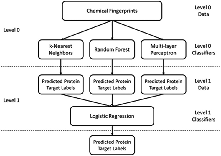
Diagram of the model stacking approach used to predict protein target labels from chemical fingerprints. Chemical fingerprints are used as input features for the level 0 classifiers: k-nearest neighbors, random forest, and multi-layer perceptron. The predicted probabilities of each protein label from each level 0 classifier are concatenated and used as input features for the level 1 classifier: logistic regression. Final predicted label probabilities are output by the logistic regression.
Model Tuning, Training, and Validation
The synthetic dataset was used for model tuning, training, and testing whereas the natural product set was used as an external test set. A stratified 10-fold cross-validation was performed on the synthetic dataset resulting in 10 folds of 90/10 split training/testing sets. The stratification process guaranteed that examples for each label were present in both the training and test cross-validation datasets. Parameters for k-nearest neighbors, random forest, and multi-layer perceptron models were tuned using the training sets for each fold. A stratified random split was used to further subdivide the training data portion of each cross-validation fold into 90/10 training/test sets for tuning. Parameters were chosen based on performance on the test tuning set (Tables S1-S3) and were then used to train all subsequent models. Following evaluation by cross-validation, the entire synthetic set was used to train models which were evaluated on the natural product dataset.
Models were trained and tested using High Performance Computing resources from the Ohio Supercomputer Center.51 Cross-validation and model combination calculations were run in parallel on the Owens cluster dense compute nodes (Dell PowerEdge C6320 two-socket servers with Intel Xeon E5-2680 v4 Broadwell, 14 cores, 2.40GHz processors, 128GB memory).
Evaluation Metrics
Area Under Receiver Operating Characteristic Curve (AUROC)
A common metric used to assess the performance of a classifier is the receiver operating characteristic (ROC) curve. Classifier predicted class probabilities, confidence values, or binary decisions are compared to the known labels. The fraction of true positives correctly recovered, the true positive rate, is plotted against the fraction of true negatives that were incorrectly identified as positive, the false positive rate. The true positive and false positive rates vary with the threshold used to split records by their probability or confidence scores into the positive and negative classes. Therefore, the true positive and false positive rates are plotted at various thresholds. The ROC curve can be summarized by a single value by calculating the area under the ROC curve. An AUROC score is represented by a value between 0 and 1, where a score of 1 denotes perfect classification, a score of 0.5 denotes random classification, and a score of 0 denotes completely incorrect classification. In general, the AUROC value can be interpreted as the probability of an active being ranked before an inactive. The AUROC score is designed for binary classification problems, but can be easily extended to multi-label classification problems by averaging over the labels. This averaging can be done through either micro- or macroaveraging. In micro-averaging, each record-label pair contributes equally to the overall score and essentially treats all labels as a single combined binary classification problem. In macro-averaging, the binary AUROC is calculated for each label and then averaged. Therefore, each label contributes equally regardless of the number of records contained.
Boltzmann-Enhanced Discrimination of Receiver Operating Characteristic (BEDROC)
While the AUROC score is a widely used and intuitive metric, it is not sensitive to early recognition. Early recognition is particularly important for target fishing problems as it is only feasible to run confirmatory experimental tests for a relatively small number of protein targets. In 2007, Truchon and Bayly proposed a metric called the Boltzmann-enhanced discrimination of receiver operating characteristic (BEDROC) to address this early recognition problem and has become a popular metric for assessing virtual screening performance.52 Similar to AUROC scores, a BEDROC score is between 0 and 1 and it has a probabilistic interpretation. However, while AUROC relates to a uniform distribution, BEDROC relates to an exponential distribution. These distributions can be considered as reference ranked lists. When a trained classifier makes predictions for a protein target label, it ultimately produces a sorted list of compounds ranked by the classifier’s confidence in a compound binding to the protein target. The AUROC or BEDROC score that this classifier sorted list receives is the probability that a known active compound randomly selected from the classifier sorted list would be ranked higher than an “active” compound randomly selected from the reference list. For the AUROC score, this reference list is random and contains “active” and “inactive” compounds uniformly distributed throughout the list. For the BEDROC score, this reference list contains a large portion of “active” compounds at the beginning of the list. When calculating the BEDROC score a parameter α is required which controls how highly “active” compounds are ranked in the reference list. For BEDROC scores to be comparable, they must use the same α value. The commonly used value is α=20 and was also used here. This α value indicates that 80% of actives are present in the first 8% of the list.
Fraction of Compounds with a True Target in the Top 10 Predictions
Because target fishing is concerned with the identification of a protein target for a given compound record, the fraction of compounds for which at least a single true target was identified in the top 10 of the ranked list was calculated. As with the BEDROC score, this score is concerned with early retrieval, however, an arbitrary cutoff of 10 predictions is used and differences in classifier performance after this cutoff will be missed. For example, a correct prediction at rank 11 is no better than a correct prediction at rank 1000 according to this metric since only correct predictions from ranks 1-10 are rewarded. Additionally this differs from the other metrics described as both AUROC and BEDROC scores were calculated from the target protein label perspective while this is calculated from the compound perspective. A cutoff of 10 targets was selected as a being a feasible number of protein targets that could be screened. This score is relatively harsh as it requires a classifier to have placed a correct target for a compound in the top 0.5% of the list in order to be rewarded, but gives an indication for the practical utility of a model for target fishing.
Coverage Error
The coverage error is a metric that is also calculated from the compound record perspective and determines on average how far down the classifier sorted list one would need to look in order to recover all true labels. The best possible value for this metric is the average number of labels for each compound record.
RESULTS AND DISCUSSION:
Natural Product Databases
There are many natural product databases or datasets that are published and available online. These databases range in size from a few hundred compounds to hundreds of thousands of compounds. A review from 2017 by Chen, Kops and Kirchmair gives a good overview of both virtual and physical natural product compound libraries.53 Many databases have a particular bioactivity focus, such as anticancer or antimalarial activities, and a focus on the geographical region from which the natural products were obtained. The smaller databases tend to have a narrow focus while the large databases attempt to aggregate and organize all known natural products, leading to significant overlap. The size and overlap of the natural product databases is shown in Figure 3. Prior to comparison, SMILES strings were standardized for each database and only unique compounds were retained, which accounts for any discrepancies between the number of compounds shown here and the published database sizes. No single database contains all of the 438,258 unique natural products that were collected. The Super Natural II database is the largest and contains 52.7% of the collected natural products. The top 5 largest databases, which include Super Natural II, Universal Natural Product Database (UNPD), ZINC Natural Products Subset, InterBioScreen (IBS) Natural Compounds, and Traditional Chinese Medicine (TCM) Database@Taiwan comprise 86.4% of the collected natural products.
Figure 3.

Size and overlap of collected natural product databases. The bar graph on the top shows the number of unique compounds in each database. The heat map shows the fraction of compounds from a database on the y-axis present in a database on the x-axis. Standardized unique SMILES strings for the compounds in each database were used for calculating size and overlap.
Synthetic Cross-Validation
Prior to benchmarking on the collected natural product data, models were trained and evaluated with the synthetic dataset using stratified 10-fold cross-validation. Overall, all trained models performed extremely well (Figure 4). Without stacking micro-averaged AUROC values ranged from 0.94 to 0.99, micro-averaged BEDROC values ranged from 0.89 to 0.94, and 89% to 92% of compounds had a true target identified in the top 10 predictions. In general, performance slightly improved when stacked. With stacking micro-averaged AUROC values ranged from 0.97 to 0.99, micro-averaged BEDROC values ranged from 0.89 to 0.97, and 85% to 95% of compounds had a true target identified in the top 10 predictions. Coverage error showed more distinct differences between different models and how stacking impacted performance. Without stacking coverage error ranged from 187 to 29 labels. Unlike the other described metrics, a lower value is better for coverage error as it represents the average number of labels that need to be considered to recover all of the true labels. With stacking this generally improved to 55 to 14 labels. The only machine learning model that did not benefit from stacking was the multilayer-perceptron (MLP). For each metric, the unstacked MLP performs better than the stacked MLP. The performance degradation is likely due to overfitting.
Figure 4.

Model performance for stratified 10-fold cross-validation on the synthetic compound dataset. For a single model, “Not Stacked” indicates that the probability predictions of the listed model were used directly. If more than one model is listed, the mean probabilities for each label were used. “Stacked” indicates that the probability predictions of the listed models were passed to the logistic regression to obtain the final predicted probabilities. Model performance as measured by (A) micro-averaged Area Under the Receiver Operating Characteristic (AUROC) curve, (B) micro-averaged Boltzmann-Enhanced Discrimination of Receiver Operating Characteristic (BEDROC), (C) the fraction of compounds which have at least one true target among the top 10 predictions, and (D) coverage error are shown.
While the performance measured for cross-validation is exemplary, it is undoubtedly an overly optimistic estimate of model performance for a prospective application. When using a random split cross-validation approach there is often redundancies between compounds present in the training and test folds. Therefore, predictions may suffer from compound series bias when predictions are made on compounds that share a scaffold with those that the model was trained on. The prediction of the correct target for a compound that is nearly identical to the training compounds is a very easy problem. Methods such as temporal split validation or clustering techniques can be used to generate more dissimilar training and testing splits to offer more realistic performance estimates.5,54,55 However, doing so requires removing activity data points and ultimately reducing the number of targets that can be considered. Consideration of a large number of targets is important to the utility of a computational target fishing method, because the method can only predict for targets it has been trained on. Despite the limitations of random splitting, other splitting techniques were not used in order to include as many target protein labels as possible.
Assessment on the natural product benchmark is expected to give a less optimistic and more realistic performance estimate. To demonstrate the difference between synthetic and natural product compounds, similarities between cross-validation training and test sets, in addition to natural product compounds, were assessed. For each protein target label, pairwise Tanimoto similarities were calculated between the training compounds themselves, training compounds with test compounds, and training compounds with the natural product benchmark compounds (Figures S2-S4). The cumulative density function (CDF) plotted for each pairwise similarity distribution is shown in Figure 5. The CDFs for the synthetic training and test sets are nearly identical. Overall, the test compounds are very similar to the training compounds and thus the good model performance observed is expected. On the other hand, the natural products are less similar and performance on this benchmark is expected to be a better indicator of realistic performance.
Figure 5.

Cumulative density function (CDF) for intra-target compound similarities. All pairwise compound similarities were calculated between the training compounds and a given set for each protein target label. “Training” and “Test” sets are from a single cross-validation fold and “Natural Product” is the natural product benchmark set.
Natural Product Benchmark
Following cross-validation, new models were trained using the entirety of the synthetic compound dataset and predictive performance was assessed for the natural product benchmark. As expected, predictive performance decreased for the natural product benchmark, especially for unstacked models (Figure 6). Without stacking micro-averaged AUROC values ranged from 0.70 to 0.85, micro-averaged BEDROC values ranged from 0.43 to 0.59, 55% to 60% of compounds had a true target identified in the top 10 predictions, and coverage error ranged from 1286 to 416. In general, model performance greatly improved when stacked. With stacking micro-averaged AUROC values ranged from 0.82 to 0.94, micro-averaged BEDROC values ranged from 0.45 to 0.73, 43% to 63% of compounds had a true target identified in the top 10 predictions, and coverage error ranged from 426 to 190. As observed in cross-validation, MLP stacked models appeared to suffer from overfitting resulting in performance degradation. While the micro-averaged AUROC value slightly increased for the MLP stacked model, all other metrics showed a performance decrease.
Figure 6.

Model performance for benchmarking on the natural product dataset. “For a single model, “Not Stacked” indicates that the probability predictions of the listed model were used directly. If more than one model is listed, the mean probabilities for each label were used. “Stacked” indicates that the probability predictions of the listed models were passed to the logistic regression to obtain the final predicted probabilities. Model performance as measured by (A) micro-averaged Area Under the Receiver Operating Characteristic (AUROC) curve, (B) micro-averaged Boltzmann-Enhanced Discrimination of Receiver Operating Characteristic (BEDROC), (C) the fraction of compounds which have at least one true target among the top 10 predictions, and (D) coverage error are shown.
Interestingly, the use of a single level 0 classifier, with the exception of MLP, saw performance improvements with model stacking. This phenomenon is particularly apparent when comparing unstacked and stacked KNN models on the natural product benchmarking set. For example, the unstacked KNN model shows the worst micro-averaged AUROC score among the unstacked classifiers, but stacking improves the score from 0.70 to 0.94. Such a dramatic increase in performance is unexpected, when the power of stacking is cited as being a result of combining level 0 classifiers. However, this assumes each model is passing singular values to be combined; either 1, 2, or 3 total values for each label depending on the number of base classifiers considered. In the models described here, all 1,907 predicted probabilities are passed from each level 0 classifier to the level 1 logistic regression classifier. Since the logistic regression is trained in a one-vs-rest fashion for this multi-label classification problem, each protein target label is predicted using all predicted probabilities; either 1,907, 3,814, or 5,721 total values for each label depending on the number of base classifiers considered. In the example of KNN, many of these predicted probabilities are 0. However, information of the non-zero values can be used to influence the prediction of a given protein target label.
The predicted target protein label information being used to give final predictions can be examined through the extraction of model coefficients from each trained logistic regression classifier. For example, the logistic regression model for predicting the protein target label “Q12884” (Prolyl endopeptidase FAP) has coefficients greater than 1 for the predicted probabilities of target labels “P48147”, “P97321”, “P27487”, “Q86TI2”, “Q9UHL4”, and “Q6V1X1’”. Inspecting the UniProt records for each reveals that these proteins share a common function, which is the cleavage of proline-containing peptide bonds. Since these proteins share a similar function and substrate preference it would be unsurprising if a given compound was able to bind to more than one of these related proteins. However, direct binding data is difficult to obtain and will be unavailable for a large number of compound-protein target combinations. Therefore, while level 0 model predictions may strongly and reasonably predict for one of these related proteins, this prediction would ultimately be treated as a false positive due to the unknown binding relationship. Through stacking, the level 1 classifier is able to learn from this information and ultimately make better predictions for the known protein target labels.
To demonstrate that the logistic regression is using probabilities of functionally related proteins to improve predictions, semantic similarities were calculated. Gene ontology (GO) is a widely used basis for the measurement of functional similarity.56-59 GO terms from the molecular function ontology were able to be obtained for 1,878 of the 1,907 UniProt protein target labels through programmatic access to QuickGO via the provided API.60 Semantic similarities for each pairwise combination of protein target label GO terms were then computed according to the Lin expression of term similarity with the best-match product method using the OntologyX package suite in R.61-64 For each predicted label, the corresponding UniProt IDs for logistic regression coefficients with values greater than one were obtained, which resulted in 1,595 label groups of the possible 1,907. The average semantic similarity of a query group of labels was calculated from the pairwise similarity matrix. Significance of group similarity for each query group of labels was assessed by a permutation test. Subsets containing the same number of labels as the query group of labels are sampled from the calculated pairwise similarity matrix. The proportion of these samples that have at least as high of an average similarity value as the query group of labels yields an unbiased estimate of the p-value for the group.65 From these calculations it is observed that 80% of the label groups had scores with associated p-values <0.05 (Figure S5). Therefore, 80% of the label groups had a similarity score higher that at least 95% of the permutated groups. Overall, the semantic similarity calculation indicates that most of protein target labels predicted by logistic regression were obtained by combination of the probabilities from functionally related proteins. This relationship was not given explicitly as an input feature during model training, but was inferred from the similarity between the training ligands for which each of the proteins were known to bind. This relationship learned by the logistic regression accounts for the highly competitive performance of the KNN classifier with the more sophisticated RF and MLP classifiers. For the synthetic set cross-validation, KNN performs very well due to the extremely high similarity between training and test compounds. However, the unstacked KNN classifier performance suffers when benchmarked on the natural product dataset that is less similar to its training data. Since KNN is a “lazy learner” and simply measures distances between a query data point and stored training data, it is expected to perform worse when evaluating dissimilar compounds.66 By applying the logistic regression to the KNN classifier predictions, the predicted probabilities for any incorrectly predicted labels may be leveraged to increase the confidence in the known target label. Therefore, the stacking KNN with logistic regression was important for improving its performance on natural products.
Impact of Training Dataset Size on Cross-Validation Performance
It is expected that the number of training records for each protein target label influences classifier performance. To assess this in a systematic way, protein class labels with a large number of compound records were collected and assessed through 10-fold cross-validation. The top 5 largest sets were selected, which included the D2 dopamine receptor (UniProtID: P14416), beta-secretase 1 (UniProtID: P56817), melanin-concentrating hormone receptor 1 (UniProtID: Q99705), cannabinoid receptor 2 (UniProtID: P34972), and vascular endothelial growth factor receptor 2 (UniProtID: P35968). A total of 2,500 compound records were randomly sampled for each protein target label and further randomly subsampled into sets of 2,000, 1,500, 1,000, 500, 100, and 10 compound records. The stratified 10-fold cross-validation procedure was then performed on each of these seven sets (Figure 7). Performance was assessed for the seven subsets using the same metrics as the original cross-validation and natural product benchmark, with the exception of true targets predicted in the top 10 results. This metric was modified to instead assess the fraction of compounds with a true target predicted as the top result.
Figure 7.

Model performance for stratified 10-fold cross-validation on datasets containing various numbers of compound training records for each protein target label for the KNN_RF classifier. For a single model, “Not Stacked” indicates that the probability predictions of the listed model were used directly. If more than one model is listed, the mean probabilities for each label were used. “Stacked” indicates that the probability predictions of the listed models were passed to the logistic regression to obtain the final predicted probabilities. Model performance as measured by (A) micro-averaged Area Under the Receiver Operating Characteristic (AUROC) curve, (B) micro-averaged Boltzmann-Enhanced Discrimination of Receiver Operating Characteristic (BEDROC), (C) the fraction of compounds which yielded a true target as the top prediction, and (D) coverage error are shown.
The number of training records for each protein target label indeed had an impact on classifier performance. As the number of training compound records increases, a corresponding increase is observed in performance. However, this effect begins to plateau at 500 compound records with a micro-averaged AUROC score of 0.999, a micro-averaged BEDROC score of 0.998, 97% of compounds had a true target identified as the top result, and a coverage error of 1.04 for the KNN_RF classifier. Additionally, “Not Stacked” and “Stacked” classifier performance converged at this point due to both achieving essentially perfect classification for the subset. The trends observed for the KNN_RF classifier were also observed for the other classifier combinations (Figures S6-S11).
Impact of Protein Target Diversity on Cross-Validation Performance
Another factor that is expected to influence performance is the diversity of protein targets in the dataset. Related protein targets are more likely to bind to similar small molecule compounds than diverse protein targets. As previously mentioned, any compound-protein target associations that were unknown were treated as negative data. This assumption has a negative impact on performance when a compound is assigned a negative label for a protein target that it may likely bind to, but has never been tested against. A classifier may reasonably predict this protein target strongly and be penalized for doing so in the performance evaluation as it is ultimately treated as a false positive prediction.
To illustrate this effect, a diverse set of protein target labels were selected from the synthetic dataset used in full model training based on their L2 protein class as defined in ChEMBL 23. A single UniProtID was selected for each L2 protein class with priority given to the protein target labels with the largest number of compound records. This resulted in a dataset containing 2,825 compound-target records for 31 diverse protein targets. Another set was obtained for comparison that contained only kinases. A total of 31 UniProtIDs were selected that belonged to the kinase L2 protein class. During UniProtID selection, labels that contained a similar number of compounds records to those selected for the diverse protein target sets were selected. This resulted in a dataset containing 2,824 compound-target records for 31 kinase protein targets.
Classifier performance was assessed by stratified 10-fold cross-validation for the two datasets using the same metrics as described for the assessment of training compound set size. The expected performance degradation when considering related targets is observed (Figure 8). Without stacking micro-averaged AUROC decreased by 0.10, micro-averaged BEDROC decreased by 0.26, 32% less compounds had a true target identified as the top prediction, and coverage error increased by 3.1 for the kinase set compared to the diverse target set. Stacking slightly improved the relative performance for micro-averaged AUROC and coverage error, and had almost no effect on micro-averaged BEDROC and the number of compounds with a true target predicted as the top result. With stacking micro-averaged AUROC decreased by 0.07, micro-averaged BEDROC decreased by 0.27, 33% less compounds had a true target identified as the top prediction, and coverage error increased by 2.4 for the kinase set compared to the diverse target set. This trend observed for the KNN_RF stacked classifier was also observed for the other classifier combinations (Figure S12). Overall, the consideration of similar targets reduces performance since the classifier more frequently predicts that a compound binds to a target for which no interaction had yet been reported.
Figure 8.

Model performance for stratified 10-fold cross-validation on the diverse target and kinase datasets for the KNN_RF classifier. For a single model, “Not Stacked” indicates that the probability predictions of the listed model were used directly. If more than one model is listed, the mean probabilities for each label were used. “Stacked” indicates that the probability predictions of the listed models were passed to the logistic regression to obtain the final predicted probabilities. Model performance as measured by (A) micro-averaged Area Under the Receiver Operating Characteristic (AUROC) curve, (B) micro-averaged Boltzmann-Enhanced Discrimination of Receiver Operating Characteristic (BEDROC), (C) the fraction of compounds which yielded a true target as the top prediction, and (D) coverage error are shown.
Impact of Intra-label Training-Test Compound Similarity on Predicted Probability Scores
Despite the use of machine learning and model stacking, this classification model is inherently dependent on ligand similarity. The underlying assumption for all ligand-based computational fishing methods is that proteins bind similar compounds. Therefore, if a query compound is dramatically dissimilar from compounds used in training the classification model for a protein target label, then low probability scores for that label are expected. Conversely, higher probability scores are expected as similarity between a query compound and the training compounds increases. However, a high degree of similarity to the training compounds is not always the case, as shown above for the natural product set, which has ramifications for the magnitude of the predicted probability scores.
To demonstrate the impact of training compound set similarity to the query compound predicted label probabilities, pairwise similarities were calculated and then compared to predicted label probability values. For each compound in the natural product benchmark set, pairwise similarities were calculated between the natural product and the training compounds belonging to the natural product’s known target label classes. This yielded a similarity distribution for each known natural product-protein target activity pair. Additionally, the predicted probabilities output by the stacked classification model for each known natural product-protein target activity pair were collected. The similarity distributions for each activity pair were aggregated and binned according the probability predicted for the known labels. The aggregated similarity distributions for each probability range are compared and shown in Figure 9 for the KNN_RF stacked classifier. For each predicted probability range bin, (0.0, 0.25], (0.25, 0.5], (0.5, 0.75], and (0.75, 1.0] the interquartile ranges span from 0.08 to 0.15, 0.10 to 0.26, 0.09 to 0.27, and 0.09 to 0.34 respectively. The lower quartile values are all very close and more distinct differences are observed between the upper quartiles especially for the lowest and highest probabilities ranges. In general, each probability range has a large proportion of low similarity values and the letter-value plots67 for each range look very similar below the median value. The major differences between distributions are observed above the median value. Comparison of the same portions of each distribution above the median, the boxes with the same width, shows an increase in average Tanimoto similarity as probability scores increase. This trend is also observed for the synthetic compound cross-validation (Figure S13) and is also more strongly observed for the non-stacked base classifiers (Figures S14-17)
Figure 9.
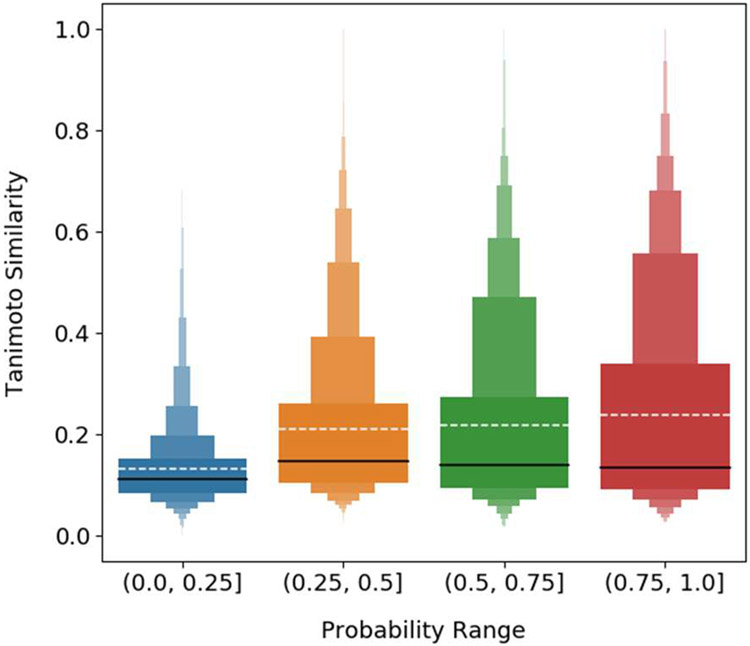
Letter-value plot showing the aggregated pairwise similarity distributions for benchmark natural product compounds and synthetic training compounds for known positive protein target labels. Similarity distributions were aggregated based on the predicted probability from the KNN_RF stacked classifier for the known protein targets of each natural product. The solid black line represents the median and the white dashed line the mean. Letter-value plots are similar to box plots, but provide more information about the tails of a distribution. Each box represents a portion of a distribution according to its width shown. The widest box is identical to the interquartile range in a box plot and represents 50% of the data. The next widest boxes, as more than one box now has identical width, comprise 25% of the data. Those boxes are present directly above and below the interquartile range. For each successive box width reduction, the amount of data represented is halved.
The number of predicted probabilities are not equally distributed among the four described ranges. There is a much larger number of probabilities predicted in the (0.0, 0.25] range, especially for the natural product set. Of the probabilities predicted by the KNN_RF stacked classifier for the natural product set, 93.8% of predicted probabilities are in the (0.0, 0.25] range, 2.8% in the (0.25, 0.5] range, 1.9% in the (0.5, 0.75] range, and 1.4 % in the (0.75, 1.0] range. For a synthetic compound cross-validation fold, 50.5% of the predicted probabilities are in the (0.0, 25] range, 9.0% are in the (0.25, 0.5] range, 9.1% are in the (0.5, 0.75] range, and 31.6% are in the (0.75, 1.0] range. Consistent with the knowledge that the synthetic compound cross-validation sets have higher intra-target similarity between training and test sets than for the natural products, the proportion of compounds receiving high probability predictions is far greater for the synthetic compounds than for the natural product set.
The observation that query compounds dissimilar from the training data yield low predicted probability scores for correct predictions has implications for model usage and interpretation. As demonstrated, the stacked classifiers had good predictive power on the natural product benchmark. Therefore, correct targets are generally ranked before incorrect targets despite the low probability scores given to correct targets. While top ranking predictions should not be taken as an absolute truth, users are also encouraged to not immediately dismiss top ranked hits based purely on a low score. No matter the score received, top ranked hits should be critically evaluated in the context of the available experimental data regarding the compounds bioactivity.
Deployment of Stacked Model as a Web Application
The trained model was deployed via an application programing interface (API) using Flask 0.12.2. The use of an API allows target predictions for molecules of interest to be made with an application run in a web browser. An example query for the natural product pukateine is shown in Figure 10. Pukateine is an aporphine alkaloid from the bark of the pukatea tree, Laurelia novae-zelandiae. Alkaloids extracted from the pukatea tree are thought to be the constituents responsible for the analgesic properties traditionally associated with the tree.68 Pukateine is reported to bind to dopamine D1 and D2 receptors. 69 When pukateine is input into the STarFish web application, dopamine D1 (UniProtID: P18901) and D2 (UniProtID: P61169) receptors are the top two predicted targets. The next two predicted targets are the 5-hydroxytryptamine receptor 2A (5-HT2A) for rat (UniProtID: P14842) and human (UniProtID: P28223). No binding data for pukateine has been reported for this receptor, however, other aporphine alkaloids have been reported to have 5-HT2A activity.70,71 Therefore, in addition to predicting two correct protein targets, STarFish, has also predicted another likely target.
Figure 10.
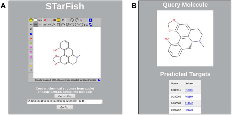
Example query using the STarFish web application. (A) Query SMILES obtained by sketching a compound or directly pasting a SMILES string into the text box. (B) The query molecule and a list of predicted protein targets along with the probability score for each.
While the KNN_RF stacked model demonstrated the best performance during cross-validation and on the natural product benchmark, the KNN stacked model was selected for use in the STarFish web application. Predictions using the RF models are significantly more computationally expensive, and the use of the KNN stacked model is computationally efficient with only a slight loss in relative performance. The use of a computationally efficient model allows for end users to easily run the STarFish web application on their own computers with minimal hardware requirements. However, experienced users are able to modify the API to include other model combinations if desired.
CONCLUSIONS:
To address how well a computational target fishing model can predict protein targets for natural products, a computational target fishing model, STarFish, was constructed using a model stacking approach and evaluated on a collected natural product benchmarking set. The collected natural product benchmark set consisted of 5,589 compound-target pairs for 1,943 unique compounds and 1,023 unique targets. All models were trained using potent synthetic compounds collected from ChEMBL and accounted for 1,907 protein targets. Model stacking combinations using k-nearest neighbors, random forest, and a multi-layer perceptron as level 0 classifiers and a logistic regression as a level 1 meta-classifier were examined. In general, model stacking approaches outperformed unstacked approaches, especially for the natural product benchmark. The stacked model comprised of KNN and RF as the level 0 classifiers showed the best performance with an AUROC score of 0.94 and a BEDROC score of 0.73. The stacked model comprised of KNN as the only level 0 classifier had similar performance with an AUROC score of 0.94 and a BEDROC score of 0.71, but with significantly less computational expense. By default, STarFish uses the stacked KNN model to allow for use even with limited computing resources and has been deployed as an API, which can downloaded and run in a web browser.
Supplementary Material
Acknowledgments
Funding Sources
The authors would like to thank the NIH for funding provided through the 2P01 CA125066 program project.
ABBREVIATIONS:
- API
application programming interface
- AUROC
area under the receiver operating characteristic
- BEDROC
Boltzmann-enhanced discrimination of receiver operating characteristic
- CDF
cumulative density function
- GO
gene ontology
- KNN
k-nearest neighbors
- MLP
multi-layer perceptron
- RF
random forest
- STarFish
stacked target fishing
Footnotes
Supporting Information
The following files are available free of charge.
Tables S1-S3. Results of base classifier tuning. Table S4. Cross-validation performance results for synthetic compound dataset. Table S5. Performance results for natural product benchmark datset. Figure S1. Comparison of the ChEMBL L2 protein classes between the synthetic compound dataset and the natural product dataset. Figures S2-S4. Comparison of intra-target pairwise compound similarities between training compounds and training, test, and natural product compounds. Figure S5. Comparison of protein functional similarity measured by semantic similarity of molecular function gene ontology (GO) ID annotations for each protein UniProt ID. Figures S6-S11. Model performance for stratified 10-fold cross-validation on datasets containing various numbers of compound training records for each protein target label for different classifier combinations. Figure S12. Model performance for stratified 10-fold cross-validation on the diverse target and kinase datasets for stacked classifiers. Figures S13-S17. Letter-value plot showing the aggregated pairwise similarity distributions for synthetic test compounds or natural product compounds and synthetic training compounds for known positive protein target labels in a cross-validation fold. Similarity distributions were aggregated based on the predicted probability from the KNN_RF stacked classifier, the KNN base classifier, or the RF base classifier for the known protein targets of each synthetic test compound. (PDF)
Snapshot of https://github.com/ntcockroft/STarFish from June 4, 2019. (ZIP)
REFERENCES:
- (1).Swinney DC; Anthony J How Were New Medicines Discovered? Nat. Rev. Drug Discov 2011, 10, 507–519. [DOI] [PubMed] [Google Scholar]
- (2).Moffat JG; Vincent F; Lee JA; Eder J; Prunotto M Opportunities and Challenges in Phenotypic Drug Discovery: An Industry Perspective. Nat. Rev. Drug Discov 2017, 16, 531–543. [DOI] [PubMed] [Google Scholar]
- (3).Oda Y; Owa T; Sato T; Boucher B; Daniels S; Yamanaka H; Shinohara Y; Yokoi A; Kuromitsu J; Nagasu T Quantitative Chemical Proteomics for Identifying Candidate Drug Targets. Anal. Chem 2003, 75, 2159–2165. [DOI] [PubMed] [Google Scholar]
- (4).Schenone M; Dančík V; Wagner BK; Clemons PA Target Identification and Mechanism of Action in Chemical Biology and Drug Discovery. Nat. Chem. Biol 2013, 9, 232–240. [DOI] [PMC free article] [PubMed] [Google Scholar]
- (5).Sydow D; Burggraaff L; Szengel A; van Vlijmen HWT; IJzerman AP; van Westen GJP; Volkamer A Advances and Challenges in Computational Target Prediction. J. Chem. Inf. Model 2019, 1728–1742. [DOI] [PubMed] [Google Scholar]
- (6).Keiser MJ; Roth BL; Armbruster BN; Emsberger P; Irwin JJ; Shoichet BK Relating Protein Pharmacology by Ligand Chemistry. Nat. Biotechnol 2007, 25, 197–206. [DOI] [PubMed] [Google Scholar]
- (7).Gaulton A; Hersey A; Nowotka M; Bento AP; Chambers J; Mendez D; Mutowo P; Atkinson F; Beilis LJ; Cibrián-Uhalte E; Davies M; Dedman N; Karlsson A; Magarinos MP; Overington JP; Papadatos G; Smit I; Leach AR The ChEMBL Database in 2017. Nucleic Acids. Res 2017, 45, D945–D954. [DOI] [PMC free article] [PubMed] [Google Scholar]
- (8).Kim S; Chen J; Cheng T; Gindulyte A; He J; He S; Li Q; Shoemaker BA; Thiessen PA; Yu B; Zaslavsky L; Zhang J; Bolton EE PubChem 2019 Lipdate: Improved Access to Chemical Data. Nucleic Acids Res. 2019, 47, D1102–D1109. [DOI] [PMC free article] [PubMed] [Google Scholar]
- (9).Svetnik V; Liaw A; Tong C; Culberson JC; Sheridan RP; Feuston BP Random Forest: A Classification and Regression Tool for Compound Classification and QSAR Modeling. J. Chem. Inf. Comput. Sci 2003, 43, 1947–1958. [DOI] [PubMed] [Google Scholar]
- (10).Burbidge R; Trotter M; Buxton B; Holden S Drug Design by Machine Learning: Support Vector Machines for Pharmaceutical Data Analysis. Comput. Chem 2001, 26, 5–14. [DOI] [PubMed] [Google Scholar]
- (11).Xia X; Maliski EG; Gallant P; Rogers D Classification of Kinase Inhibitors Using a Bayesian Model. J. Med. Chem 2004, 47, 4463–4470. [DOI] [PubMed] [Google Scholar]
- (12).Mayr A; Klambauer G; Unterthiner T; Steijaert M; Wegner JK; Ceulemans H; Clevert D-A; Hochreiter S Large-Scale Comparison of Machine Learning Methods for Drug Target Prediction on ChEMBL. Chem. Sci. 2018, 9, 5441–5451. [DOI] [PMC free article] [PubMed] [Google Scholar]
- (13).Rifaioglu AS; Atas H; Martin MJ; Cetin-Atalay R; Atalay V; Doğan T Recent Applications of Deep Learning and Machine Intelligence on in Silico Drug Discovery: Methods, Tools and Databases. Brief. Bioinform 44, 1–36. [DOI] [PMC free article] [PubMed] [Google Scholar]
- (14).Newman DJ; Cragg GM Natural Products as Sources of New Drugs from 1981 to 2014. J. Nat. Prod 2016, 79, 629–661. [DOI] [PubMed] [Google Scholar]
- (15).Eder J; Sedrani R; Wiesmann C The Discovery of First-in-Class Drugs: Origins and Evolution. Nat. Rev. DrugDiscov 2014, 13, 577–587. [DOI] [PubMed] [Google Scholar]
- (16).Reker D; Rodrigues T; Schneider P; Schneider G Identifying the Macromolecular Targets of de Novo-Designed Chemical Entities through Self-Organizing Map Consensus. PNAS 2014, 111, 4067–4072. [DOI] [PMC free article] [PubMed] [Google Scholar]
- (17).Reker D; Pema AM; Rodrigues T; Schneider P; Reutlinger M; Mönch B; Koeberle A; Lamers C; Gabler M; Steinmetz H; Müller R; Schubert-Zsilavecz M; Werz O; Schneider G Revealing the Macromolecular Targets of Complex Natural Products. Nature Chemistry 2014, 6, 1072–1078. [DOI] [PubMed] [Google Scholar]
- (18).Rodrigues T Harnessing the Potential of Natural Products in Drug Discovery from a Cheminformatics Vantage Point. Org. Biomol. Chem 2017, 75, 9275–9282. [DOI] [PubMed] [Google Scholar]
- (19).Fang J; Wu Z; Cai C; Wang Q; Tang Y; Cheng F Quantitative and Systems Pharmacology. 1. In Silico Prediction of Drug–Target Interactions of Natural Products Enables New Targeted Cancer Therapy. J. Chem. Inf. Model 2017, 57, 2657–2671. [DOI] [PMC free article] [PubMed] [Google Scholar]
- (20).Keum J; Yoo S; Lee D; Nam H Prediction of Compound-Target Interactions of Natural Products Using Large-Scale Drug and Protein Information. BMC Bioinformatics 2016, 17. [DOI] [PMC free article] [PubMed] [Google Scholar]
- (21).Grenet I; Merlo K; Comet J-P; Tertiaux R; Rouquié D; Dayan F Stacked Generalization with Applicability Domain Outperforms Simple QSAR on in Vitro Toxicological Data. J. Chem. Inf. Model 2019. [DOI] [PubMed] [Google Scholar]
- (22).Li W; Miao W; Cui J; Fang C; Su S; Li H; Hu L; Lu Y; Chen G Efficient Corrections for DFT Noncovalent Interactions Based on Ensemble Learning Models. J. Chem. Inf. Model 2019. [DOI] [PubMed] [Google Scholar]
- (23).Kaggle: Your Home for Data Science https://www.kaggle.com/ (accessed Apr 18, 2019).
- (24).Otto Group Product Classification Challenge https://kaggle.com/c/otto-group-product-classification-challenge (accessed Apr 18, 2019).
- (25).Afzal AM; Mussa HY; Turner RE; Bender A; Glen RC A Multi-Label Approach to Target Prediction Taking Ligand Promiscuity into Account. J. Cheminform 2015, 7. [DOI] [PMC free article] [PubMed] [Google Scholar]
- (26).Ntie-Kang F; Simoben CV; Karaman B; Ngwa VF; Judson PN; Sippl W; Mbaze LM Pharmacophore Modeling and in Silico Toxicity Assessment of Potential Anticancer Agents from African Medicinal Plants. Drug Des. Devel. Ther 2016, 10, 2137–2154. [DOI] [PMC free article] [PubMed] [Google Scholar]
- (27).Ntie-Kang F; Zofou D; Babiaka SB; Meudom R; Scharfe M; Lifongo LL; Mbah JA; Mbaze LM; Sippl W; Efange SMN AfroDb: A Select Highly Potent and Diverse Natural Product Library from African Medicinal Plants. PLOS ONE 2013, 8, e78085. [DOI] [PMC free article] [PubMed] [Google Scholar]
- (28).Onguéné PA; Ntie-Kang F; Mbah JA; Lifongo LL; Ndom JC; Sippl W; Mbaze LM The Potential of Anti-Malarial Compounds Derived from African Medicinal Plants, Part III: An in Silico Evaluation of Drug Metabolism and Pharmacokinetics Profiling. Org. Med. Chem. Lett 2014, 4, 6. [DOI] [PMC free article] [PubMed] [Google Scholar]
- (29).Natural Resources and Technologies https://ac-discovery.com/ (accessed Dec 19, 2018).
- (30).Yabuzaki J Carotenoids Database: Structures, Chemical Fingerprints and Distribution among Organisms. Database (Oxford) 2017, 2017. [DOI] [PMC free article] [PubMed] [Google Scholar]
- (31).Ntie-Kang F; Onguéné PA; Scharfe M; Owono LCO; Megnassan E; Mbaze LM; Sippl W; Efange SMN ConMedNP: A Natural Product Library from Central African Medicinal Plants for Drug Discovery. RSC Adv. 2013, 4, 409–419. [Google Scholar]
- (32).InterBioScreen ltd. ∣ Compound Libraries https://www.ibscreen.com (accessed Dec 19, 2018).
- (33).MITISHAMBA DATABASE http://mitishamba.uonbi.ac.ke/ (accessed Dec 19, 2018).
- (34).Ntie-Kang F; Telukunta KK; Döring K; Simoben CV; A. Moumbock a.f.; Malange YI; Njume LE; Yong JN; Sippl W; Günther S NANPDB: A Resource for Natural Products from Northern African Sources. J. Nat. Prod. 2017, 80, 2067–2076. [DOI] [PubMed] [Google Scholar]
- (35).Natural Products Atlas ∣ Home https://www.npatlas.org/joomla/index.php (accessed Dec 19, 2018).
- (36).Mangal M; Sagar P; Singh H; Raghava GPS; Agarwal SM NPACT: Naturally Occurring Plant-Based Anti-Cancer Compound-Activity-Target Database. Nucleic Acids Res. 2013, 41, D1124–D1129. [DOI] [PMC free article] [PubMed] [Google Scholar]
- (37).Zeng X; Zhang P; He W; Qin C; Chen S; Tao L; Wang Y; Tan Y; Gao D; Wang B; Chen Z; Chen W; Jiang YY; Chen YZ NPASS: Natural Product Activity and Species Source Database for Natural Product Research, Discovery and Tool Development. Nucleic Acids Res. 2018, 46, D1217–D1222. [DOI] [PMC free article] [PubMed] [Google Scholar]
- (38).Pilon AC; Valli M; Dametto AC; Pinto MEF; Freire RT; Castro-Gamboa I; Andricopulo AD; Bolzani VS NuBBE DB : An Updated Database to Uncover Chemical and Biological Information from Brazilian Biodiversity. Sci. Rep 2017, 7, 7215. [DOI] [PMC free article] [PubMed] [Google Scholar]
- (39).Ntie-Kang F; Onguéné PA; Fotso GW; Andrae-Marobela K; Bezabih M; Ndom JC; Ngadjui BT; Ogundaini AO; Abegaz BM; Meva’a LM Virtualizing the P-ANAPL Library: A Step towards Drug Discovery from African Medicinal Plants. PLOS ONE 2014, 9, e90655. [DOI] [PMC free article] [PubMed] [Google Scholar]
- (40).Hatherley R; Brown DK; Musyoka TM; Penkler DL; Faya N; Lobb KA; Tastan Bishop Ö SANCDB: A South African Natural Compound Database. J. Cheminform. 2015, 7. [DOI] [PMC free article] [PubMed] [Google Scholar]
- (41).Banerjee P; Erehman J; Gohlke B-O; Wilhelm T; Preissner R; Dunkel M Super Natural II—a Database of Natural Products. Nucleic Acids Res. 2015, 43, D935–D939. [DOI] [PMC free article] [PubMed] [Google Scholar]
- (42).Chen CY-C TCM Database@Taiwan: The World’s Largest Traditional Chinese Medicine Database for Drug Screening In Silico. PLOS ONE 2011, 6. [DOI] [PMC free article] [PubMed] [Google Scholar]
- (43).Lin Y-C; Wang C-C; Chen I-S; Jheng J-L; Li J-H; Tung C-W TlPdb: A Database of Anticancer, Antiplatelet, and Antituberculosis Phytochemicals from Indigenous Plants in Taiwan https://www.hindawi.com/journals/tswj/2013/736386/ (accessed Dec 19, 2018). [DOI] [PMC free article] [PubMed]
- (44).Gu J; Gui Y; Chen L; Yuan G; Lu H-Z; Xu X Use of Natural Products as Chemical Library for Drug Discovery and Network Pharmacology. PLOS ONE 2013, 8. [DOI] [PMC free article] [PubMed] [Google Scholar]
- (45).Sterling T; Irwin JJ ZINC 15 – Ligand Discovery for Everyone. J. Chem. Inf. Model 2015, 55, 2324–2337. [DOI] [PMC free article] [PubMed] [Google Scholar]
- (46).MolVS: Molecule Validation and Standardization — MolVS 0.1.1 documentation https://molvs.readthedocs.io/en/latest/ (accessed Dec 20, 2018).
- (47).Peón A; Naulaerts S; Ballester PJ Predicting the Reliability of Drug-Target Interaction Predictions with Maximum Coverage of Target Space. Sci. Rep 2017, 7, 3820. [DOI] [PMC free article] [PubMed] [Google Scholar]
- (48).RDKit: Open-source cheminformatics; https://www.rdkit.org/ (accessed Dec 20, 2018).
- (49).Rogers D; Hahn M Extended-Connectivity Fingerprints../. Chem. Inf. Model 2010, 50, 742–754. [DOI] [PubMed] [Google Scholar]
- (50).Pedregosa F Scikit-Learn: Machine Learning in Python. MACHINE LEARNING IN PYTHON 6. [Google Scholar]
- (51).Ohio Supercomputer Center. 1987.
- (52).Truchon J-F; Bayly CI Evaluating Virtual Screening Methods: Good and Bad Metrics for the “Early Recognition” Problem. J. Chem. Inf. Model 2007, 47, 488–508. [DOI] [PubMed] [Google Scholar]
- (53).Chen Y; de Bruyn Kops C; Kirchmair J Data Resources for the Computer-Guided Discovery of Bioactive Natural Products. J. Chem. Inf. Model 2017, 57, 2099–2111. [DOI] [PubMed] [Google Scholar]
- (54).Lopez-del Rio A; Nonell-Canals A; Vidal D; Perera-Lluna A Evaluation of Cross-Validation Strategies in Sequence-Based Binding Prediction Using Deep Learning. J. Chem. Inf. Model 2019. [DOI] [PubMed] [Google Scholar]
- (55).Lenselink EB; Dijke N.ten; Bongers B; Papadatos G; Vlijmen H. W. T. van; Kowalczyk W; IJzerman AP; Westen G. J. P. van. Beyond the Hype: Deep Neural Networks Outperform Established Methods Using a ChEMBL Bioactivity Benchmark Set. J. Cheminform 2017, 9, 45. [DOI] [PMC free article] [PubMed] [Google Scholar]
- (56).Teng Z; Guo M; Liu X; Dai Q; Wang C; Xuan P Measuring Gene Functional Similarity Based on Group-Wise Comparison of GO Terms. Bioinformatics 2013, 29, 1424–1432. [DOI] [PubMed] [Google Scholar]
- (57).Weichenberger CX; Palermo A; Pramstaller PP; Domingues FS Exploring Approaches for Detecting Protein Functional Similarity within an Orthology-Based Framework. Sci. Rep 2017, 7, 381. [DOI] [PMC free article] [PubMed] [Google Scholar]
- (58).Mazandu GK; Mulder NJ Information Content-Based Gene Ontology Functional Similarity Measures: Which One to Use for a Given Biological Data Type? PLOS ONE 2014, 9, el 13859. [DOI] [PMC free article] [PubMed] [Google Scholar]
- (59).Liu M; Thomas PD GO Functional Similarity Clustering Depends on Similarity Measure, Clustering Method, and Annotation Completeness. BMC Bioinformatics 2019, 20, 155. [DOI] [PMC free article] [PubMed] [Google Scholar]
- (60).Binns D; Dimmer E; Huntley R; Barrell D; O’Donovan C; Apweiler R QuickGO: A Web-Based Tool for Gene Ontology Searching. Bioinformatics 2009, 25, 3045–3046. [DOI] [PMC free article] [PubMed] [Google Scholar]
- (61).RStudio Team (2015). RStudio: Integrated Development for R. RStudio, Inc., Boston, MA: URL Http://www.Rstudio.com/. [Google Scholar]
- (62).R Development Core Team (2008). R: A Language and Environment Statistical Computing. R Foundation for Statistical Computing, Vienna, Austria: ISBN 3-900051-07-0, URL Http://Www.R-Project.org. [Google Scholar]
- (63).Greene D; Richardson S; Turro E OntologyX: A Suite of R Packages for Working with Ontological Data. Bioinformatics 2017, 33, 1104–1106. [DOI] [PMC free article] [PubMed] [Google Scholar]
- (64).Lin D An Information-Theoretic Definition of Similarity. In In Proceedings of the 15th International Conference onMachine Learning, Morgan Kaufmann, 1998; pp 296–304. [Google Scholar]
- (65).Greene DJ Methods for Determining the Genetic Causes of Rare Diseases, University of Cambridge, 2018. [Google Scholar]
- (66).Veenman CJ; Reinders MJT The Nearest Subclass Classifier: A Compromise between the Nearest Mean and Nearest Neighbor Classifier. IEEE Transactions on Pattern Analysis and Machine Intelligence 2005, 27, 1417–1429. [DOI] [PubMed] [Google Scholar]
- (67).Hofmann H; Wickham H; Kafadar K Letter-Value Plots: Boxplots for Large Data. J. Comput. Graph. Stat 2017, 26, 469–477. [Google Scholar]
- (68).Fogg WS The Pharmacological Action of Pukateine. J. Pharmacol. Exp. Ther 1935, 54, 167–187. [Google Scholar]
- (69).Dajas-Bailador FA; Asencio M; Bonilla C; Scorza Ma. C.; Echeverry C; Reyes-Parada M; Silveira R; Protais P; Russell G; Cassels BK; Dajas F Dopaminergic Pharmacology and Antioxidant Properties of Pukateine, a Natural Product Lead for the Design of Agents Increasing Dopamine Neurotransmission. Gen. Pharmacol 1999, 32, 373–379. [DOI] [PubMed] [Google Scholar]
- (70).Munusamy V; Yap BK; Buckle MJC; Doughty SW; Chung LY Structure-Based Identification of Aporphines with Selective 5-HT2A Receptor-Binding Activity. Chem. Biol. Drug Des 2013, 81, 250–256. [DOI] [PubMed] [Google Scholar]
- (71).Ponnala S; Gonzales J; Kapadia N; Navarro HA; Harding WW Evaluation of Structural Effects on 5-HT2A Receptor Antagonism by Aporphines: Identification of a New Aporphine with 5-HT2A Antagonist Activity. Bioorg. Med. Chem. Lett 2014, 24, 1664–1667. [DOI] [PMC free article] [PubMed] [Google Scholar]
Associated Data
This section collects any data citations, data availability statements, or supplementary materials included in this article.