

Abstract
Statistical significance tests are a common feature in quantitative proteomics workflows. The Student’s t-test is widely used to compute the statistical significance of a protein’s change between two groups of samples. However, the t-test’s null hypothesis asserts that the difference in means between two groups is exactly zero, often marking small but uninteresting fold-changes as statistically significant. Compensations to address this issue are widely used in quantitative proteomics, but we suggest that a replacement of the t-test with a Bayesian approach offers a better path forward. In this article, we describe a Bayesian hypothesis test in which the null hypothesis is an interval rather than a single point at zero; the width of the interval is estimated from population statistics. The improved sensitivity of the method substantially increases the number of truly changing proteins detected in two benchmark data sets (ProteomeXchange identifiers PXD005590 and PXD016470). The method has been implemented within FlashLFQ, an open-source software program that quantifies bottom-up proteomics search results obtained from any search tool. FlashLFQ is rapid, sensitive, and accurate, and is available as both an easy-to-use graphical user interface (Windows) and as a command line tool (Windows/Linux/OSX).
Keywords: label-free quantification, software, quantitative proteomics, Bayesian statistics, Bayesian hypothesis test
Graphical Abstract
INTRODUCTION
The goal of quantitative proteomics is to identify and quantify the proteins in a given sample[1]. In a typical bottom-up mass spectrometry-based workflow, proteins are digested with an enzyme and the resulting peptide mixture is injected into an LC-MS/MS system. The acquired mass spectrometry data are usually analyzed by informatics software; peptides are first identified from their fragmentation (MS2) spectra using a search engine, and the proteins likely to be present in the sample are then inferred from the identified peptides using the principle of Occam’s razor[2][3]. Peptides are quantified by, for example, MS1 intensity, MS2 fragment intensities, MS2-based label intensities, or simply by counting the number of MS2 spectra assigned to a given peptide. Protein quantities are then estimated from the peptide-level quantitative data. This is usually a relative quantification; in other words, the quantity being measured is a change in protein abundance between two or more groups of samples and not an absolute abundance. Lastly, the statistical significance of a protein’s change is estimated, with quantitative false positives controlled by false discovery rate (FDR) estimation.
There are many software tools that perform one or more stages of this process, including MaxQuant[4], Perseus[5], moFF[6], ProStar/DAPAR[7], and others[8][9][10][11][12][13][14][15]. We have previously described an algorithm for rapid label-free peptide quantification and implemented it in FlashLFQ, a free, open-source software program[16]. We have since added significant functionality to FlashLFQ that includes intensity normalization, match-between-runs, relative protein quantification, and hypothesis testing.
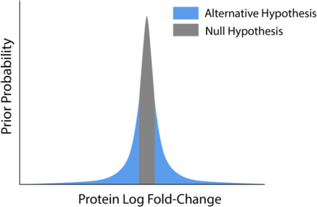
Hypothesis testing is used to determine the statistical significance of a protein’s fold-change between sample groups. Student’s t-test[17] is typically used for this purpose. This procedure has its flaws, however. It has long been observed[18] that many analytes have precise, statistically significant changes in abundance between groups, but which have small effect sizes (e.g., a protein with a log-change of 0.01 ± 0.001). The statistical significance of such a result highlights a problem with the t-test’s null hypothesis, which asserts that the difference in means of the groups is exactly zero. In a set of distinct physical samples, it is a virtual certainty that the mean of any protein change will not be exactly equal to zero; and even if the difference is exactly zero, given enough data, this null hypothesis is always rejected[19]. For this reason, many quantitative proteomics workflows employ a “fold-change cutoff” to filter out proteins with a log-change less than a certain magnitude. While this procedure does resolve some issues with Student’s t-test, it creates new problems of its own. This filter rejects proteins with means slightly inside the cutoff and accepts proteins with means slightly outside the cutoff, without regard to uncertainty in the estimate of the mean. This decreases sensitivity (i.e., it reduces the ability to detect truly changing proteins) because many proteins inside the cutoff have non-negligible probabilities that their means are outside the cutoff. Additionally, this cutoff does not change the t-test’s null hypothesis; the p-value resulting from the t-test is thus not indicative of statistical significance with regard to the cutoff. This decreases the interpretability of the already commonly-misinterpreted[20] p-value. Improved versions of the t-test exist,[15] which incorporate a fold-change cutoff into the null hypothesis itself. However, Bayesian statistics offers more intuitively understandable results and more flexibility in the underlying data model than the t-test.
Instead of attempting to compensate for the t-test’s shortcomings, we have developed a Bayesian hypothesis test which estimates the probability that the protein’s log-change magnitude is below some threshold. This manuscript adds to the growing body of work which uses Bayesian statistics in protein quantification[11][21][22].
Bayesian statistics is based on Bayes’ rule, which calculates the probability of an event having occurred given an initial probability of the event occurring and evidence of the event. The probability before taking evidence into account is called the prior probability. From the perspective of protein quantification, one can ask, “what is the probability that this protein’s fold-change is X?” One would be hard-pressed to answer that question without prior knowledge of the system under study. One could choose many different values for X and arrive at essentially the same non-conclusive result. This forms the logical basis for a diffuse (often called “uninformative”) prior probability distribution; for any particular value of X, the prior probability is essentially the same. Formally, this diffuse prior is justified by the principle of indifference, which states that credibility should be allocated equally among possibilities before evidence is taken into account[23][24]. The probability after the evidence is factored in is called the posterior probability. Bayes’ rule can be used to produce a posterior probability for each value of X that one chooses. This forms a posterior probability distribution. Technically, a quantity proportional to the posterior probability called the likelihood is computed instead of the posterior probability. The integral of the likelihood space is needed to normalize the likelihood to a probability; this integral is commonly difficult or impossible to compute. However, there are several methods to iteratively sample values of X and calculate their likelihoods such that a histogram of values approximates the posterior probability distribution. We use one such method (specifically, a Markov chain Monte Carlo algorithm[25][26]), to sample the posterior probability space in order to answer two questions for each protein:
How much is the protein changing between conditions?
Is the protein’s magnitude of change above some threshold T0?
We argue that these two questions should be answered starting from two different prior probability distributions. The first question’s prior probability distribution should be diffuse, as justified above. The second question is a binary choice between an interval null hypothesis[27] H0, which asserts that the protein’s mean change between two groups (µ2 - µ1) is below the threshold (H0 = -T0 < µ2 - µ1 < T0) and an alternative hypothesis Ha, which asserts that the mean change is outside the threshold (Ha = µ2 - µ1 > T0 or µ2 - µ1 < -T0). Using the principle of indifference, the prior probability distribution for μ should have 50% of its probability density contained within the interval and 50% outside of it.
A distinction between the present work and previous Bayesian approaches is the elimination of the requirement of an unchanging background of proteins to be present in any sample (though this background is needed for FlashLFQ’s normalization). Another difference is that we describe and implement a method which scales T0 (i.e., the width of the interval null hypothesis) with uncertainty in the data. We show that this empirically-derived null hypothesis strategy controls the FDR while maintaining sensitivity to truly changing proteins in two benchmark data sets.
FlashLFQ is a free, open-source label-free quantification program and is available via GitHub (https://github.com/smith-chem-wisc/FlashLFQ) as a graphical user interface (Windows) or command-line program (Windows, Linux, or OSX). It is designed to accept peptide identification input from any search program. FlashLFQ is also bundled with the search software program MetaMorpheus (https://github.com/smith-chem-wisc/MetaMorpheus), which allows the easy discovery and quantification of post-translationally modified peptides. The command-line version of FlashLFQ is also available in a Docker container (https://hub.docker.com/r/smithchemwisc/flashlfq).
EXPERIMENTAL METHODS
All analyses were performed on a Dell Precision Tower 5810 desktop computer with a 6-core, 12-thread Xeon 3.60 GHz processor and 31.9 GB of RAM. See Supporting Methods for additional details about algorithms used in FlashLFQ.
Estimation of protein fold-change.
FlashLFQ estimates each protein’s fold-change from its constituent peptides’ fold-changes. The estimated mean of the peptide fold-changes is interpreted as the protein’s fold-change; this mean is estimated using Bayesian statistics. The intensities of the peptides assigned to a protein are first log-transformed and then scaled via a relative ionization efficiency estimation. The relative ionization efficiency of a peptide is approximated by taking the median of the peptide’s (log-scaled) measurements in the first sample group; subsequently, this value is subtracted from all of that peptide’s measurements across the sample groups. A Bayesian method developed by Kruschke[19] is used to estimate the mean (µ), scale (σ, akin to the standard deviation), and degree of normality (ν, sometimes called “degrees of freedom”) parameters of each sample group of peptide abundance measurements. This strategy involves generating a series of Student’s t-distributions and calculating the relative likelihood that each t-distribution represents the data. The algorithm randomly generates t-distributions and adapts towards more likely t-distributions with each iteration. The generation and iterative adaptation of these t-distributions is achieved by use of an adaptive Metropolis-within-Gibbs Markov Chain Monte Carlo (MCMC) algorithm[26]. The purpose of generating these t-distributions is to sample from the posterior probability distribution, not to fit the single best t-distribution. In other words, µ, σ, and ν of the peptide measurements should be viewed as each having a range of possibilities rather than a single value. The parameter values for each t-distribution are collected into a histogram; for example, 3000 iterations of the MCMC algorithm would produce 3000 t-distributions, each having a µ, σ, and ν value. Because this algorithm adapts towards more likely parameter values, more likely parameter values will be sampled more often. The resulting histograms approximate the posterior probability distribution for each parameter. The (relative) likelihood of an individual t-distribution representing the data is calculated by multiplying the probability densities (y-values of the t-distribution) at each peptide measurement (x-values). The likelihood of the t-distribution representing the data is multiplied by the prior probability of each of the t-distribution’s parameters. Because any given fold-change is not particularly likely without evidence, we use a diffuse prior probability distribution for µ. By default, FlashLFQ generates 4000 t-distributions and discards the first 1000. The number of iterations can be increased to achieve arbitrary precision of the posterior probability distributions for each parameter at the cost of computation time. The point estimate for each of the three parameters (µ, σ, and ν) is taken as the median value of the corresponding posterior probability distribution. As described in the introduction, it is important to use a diffuse prior for µ when estimating the protein’s fold-change; by contrast, using a prior concentrated around 0 results in the magnitude of the fold-change being underestimated (Supporting Information Figure 3).
Hypothesis testing.
Our procedure for performing a Bayesian hypothesis test is essentially identical to the preceding section, except that the prior probability distribution for μ is concentrated around zero. In this hypothesis test, the null hypothesis is an interval from -T0 to T0. We refer to “T0” as half the width of the symmetric null interval; in other words, if the null interval ranges from −0.5 to 0.5, then T0 = 0.5. The key to performing this test is to construct the priors for µ1 and µ2 such that 50% of the prior probability density of the difference in means falls within the interval null hypothesis (see Supporting Methods 6 for details about how these priors are constructed; see Supporting Information Figure S2 for erroneous anticonservative results that arise from using a diffuse prior for µ in the hypothesis test). The posterior probability distributions are then sampled via the MCMC method described above. The probability that the protein’s change is below the threshold (i.e., that the null hypothesis is true, ) is the integrated area under the posterior probability distribution where -T0 < µ2 - µ1 < T0. The probability of the alternative hypothesis, , is the area outside the null interval. The ratio is called the Bayes Factor; this ratio is computed for each hypothesis test. A method by Wen[28] is used to compute the false discovery rate from a collection of Bayes Factors. The estimated proportion of true null hypotheses, , is calculated by ranking the Bayes Factors in ascending order, finding the largest set where the average is less than one, then dividing the number of tests in this set by the total number of tests. The quantity , where BF is the Bayes Factor of a test, is the posterior probability that accepting the test would result in a false-positive (the posterior error probability, or PEP). The false discovery rate of a set of tests is the average PEP of the set.
Determination of the interval null hypothesis width.
The width of the null hypothesis interval is an important parameter in this analysis. The null hypothesis needs to be wide enough so that proteins that are not changing in abundance are marked as confidently not changing; estimating the proportion of the data which comprises the unchanging background () is an important factor in calculating the false-discovery rate. However, what comprises “background” is partially subjective. For example, one may wish to perform biochemical validations of protein abundance changes between conditions and, given limited resources to perform such tasks, require that proteins be at least doubling in abundance with high confidence. Others may wish to publish a more complete list of proteins whose detected changes are unlikely to be caused by noise in the data. We combine these subjective and uncertainty-driven approaches by calculating the uncertainty in µ2 – µ1 for each protein and using the larger of half of this value or the user-defined cutoff as T0.
Intensity-Dependent Prior for σ.
The accuracy in the final determination of a statistically significant fold-change depends strongly on achieving a good estimate for the prior of σ, especially in cases where the number of observed measurements is low. In these cases, stochastic variation in individual measurements can result in the variance for a particular protein’s measurements being artificially low or artificially high by random chance. Thus, it is an improvement to complement the measurements for the protein with a prior for σ constructed from a larger population of peptides with similar intensities as the protein’s. We first tabulate all measured peptide intensities across the samples for the sample group, sorted by intensity. In sets of 100 peptides, we determine the median peptide variance for the set. This value is used to represent the typical variance of a peptide with intensity i (σ2i). To propagate this information to the protein level, we can view the protein as a pooled set of peptide measurements (e.g., 3 peptides with 3 measurements each, for a total of 9 measurements in the pool). The equation for pooled variance[29] is used to aggregate the σ2i values into a pooled estimate for the variance of the protein, given its constituent peptide intensities (σ2pool). Supporting Methods 7 contains a detailed description of this calculation.
Data sets.
Two benchmark data sets were used for this analysis, one composed of unfractionated samples and another composed of fractionated samples. Each data set contained two groups of samples. The first group contained a mixture of E. coli and human protein digest, and the second group contained a similar mixture except that the amount of E. coli was twice the amount as the first group. Thus, the ground truth of protein change is known; E. coli proteins are changing between the two groups of samples and human proteins are not. The unfractionated samples were acquired by the Qu group (data set identifier PXD005590)[30] and the fractionated samples were separately prepared in-house. The mass spectrometry proteomics data have been deposited to the ProteomeXchange Consortium via the PRIDE[31] partner repository with the dataset identifier PXD016470. Additional details about the samples (growth conditions, etc.) are included in Supporting Methods 3. For review only: the fractionated data set acquired for thismanuscript can be accessed with the username reviewer68201@ebi.ac.uk and the password mBUVDYuA on http://www.proteomexchange.org/.
Software.
FlashLFQ:
FlashLFQ version 1.1.1 was used for all analyses. FlashLFQ settings: normalization was enabled; match-between-runs was enabled; Bayesian fold-change analysis was enabled; shared peptides were not used for protein quantification; the random seeds were automatically generated as 1949466410 for the fractionated data set and −2091165151 for the unfractionated data set. The experimental design for the fractionated data, which specifies each spectra file’s condition, sample number, fraction number, and replicate number is described in Supporting Methods 4. The peptide identification results from the Andromeda search engine within MaxQuant were imported into FlashLFQ in order to control for peptide identifications; in other words, the same set of peptides was quantified by FlashLFQ and MaxQuant so as to only compare the quantitative algorithms of the two software programs, rather than using a different peptide search engine, which would introduce additional variables.
MaxQuant:
MaxQuant version 1.6.7.0 was used for all analyses. MaxQuant settings: oxidation of methionine and acetylation of protein N-terminus were used as variable modifications; carbamidomethylation of cysteine was used as a fixed modification; “LFQ” was selected as the label-free quantification option; match-between-runs was enabled; peptides used for protein quantification was set to “unique”; 1 processor was used.
Perseus:
Perseus version 1.6.7.0 was used for all analyses. False discovery rate estimation was performed via permutation with 250 permutations (Figures 3 and 4) or via Benjamini-Hochberg correction (Supporting Information Figure S1). Five different combinations of filtering based on valid values and imputation were performed (Perseus strategies 1 through 5, summarized in Table 1), and several values for the “s0” fold-change cutoff parameter were tested for each strategy. Data presented in figures of this manuscript used values of s0 which estimated the false discovery proportion (FDP) accurately while also providing the highest sensitivity. All data resulting from the different filtering and imputation strategies, along with tested values for s0, are provided in Supporting Information Table S2.
Figure 3.
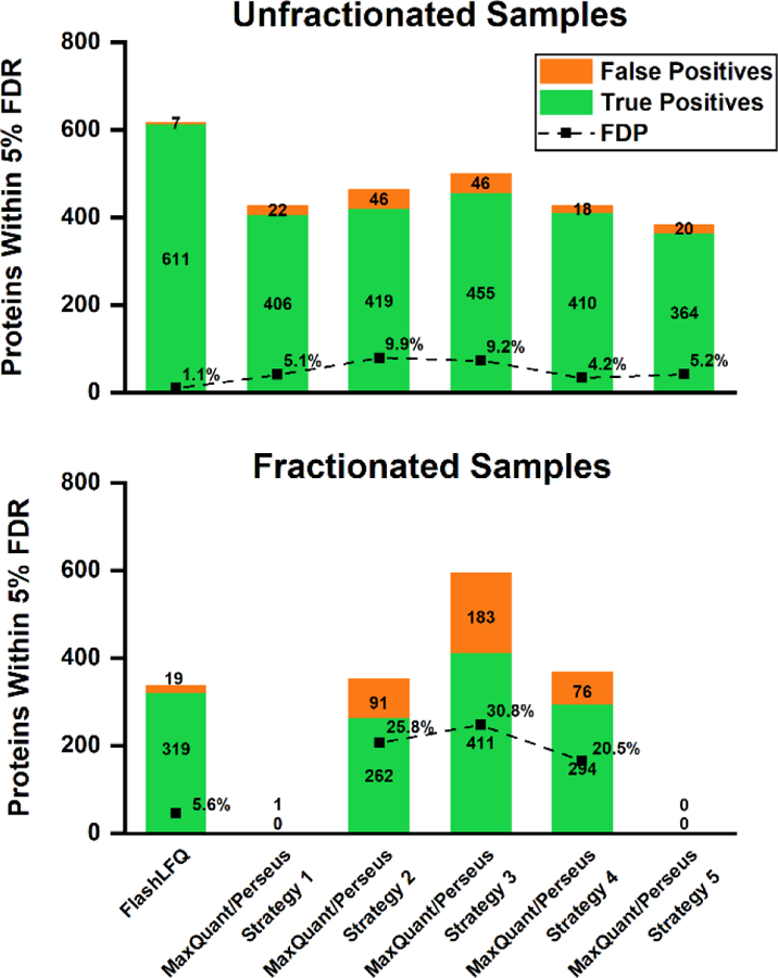
False positive (human) and true positive (E. coli) proteins detected as changing by either FlashLFQ or various MaxQuant/Perseus strategies, at an estimated 5% FDR, along with FDP for each strategy (see Table 1 for descriptions of these strategies). FlashLFQ and MaxQuant/Perseus controlled the FDP well in the unfractionated samples, though FlashLFQ was more sensitive; in the fractionated samples, MaxQuant/Perseus either had low sensitivity (strategies 1 and 5) or high FDPs (strategies 2, 3, and 4). By contrast, FlashLFQ controlled the FDP and detected 319 truly changing proteins in the high-uncertainty fractionated data set.
Figure 4.

MaxQuant results analyzed with Bayesian-estimated FDR, compared to FDR estimated via t-test, permutation, and a fold-change cutoff. Bayesian-estimated FDR results in an increased sensitivity and accurate FDR estimation for both the unfractionated and fractionated samples compared to the frequentist method.
Table 1.
| Strategy | Filtering on valid values | Missing value imputation | False Discovery Rate Estimation |
|---|---|---|---|
| Strategy 1 | 3 valid values in total | Imputed from total matrix with width=0.5, down-shift=1.5 | Permutation; num. randomizations = 250 |
| Strategy 2 | 4 valid values in at least one group | Imputed from total matrix with width=0.5, down-shift=1.5 | Permutation; num. randomizations = 250 |
| Strategy 3 | 2 valid values from both groups (required to perform the t-test) | No imputation | Permutation; num. randomizations = 250 |
| Strategy 4 | 2 valid values in both groups | Imputed from total matrix with width=0.5, down-shift=1.5 | Permutation; num. randomizations = 250 |
| Strategy 5 | No filter | Imputed from total matrix with width=0.5, down-shift=1.5 | Permutation; num. randomizations = 250 |
RESULTS AND DISCUSSION
Comparison of MaxQuant’s and FlashLFQ’s estimated protein fold-changes
We first evaluated the accuracy of FlashLFQ’s estimated protein fold-changes. Two benchmark data sets were used in which the samples consisted of small amounts of E. coli digest added to a large amount of human digest. Each data set had two groups of samples; in one of the groups, the samples had twice the amount of E. coli digest as the first. One data set’s samples were fractionated and the other’s were unfractionated. A perfect quantitative analysis would indicate all E. coli proteins doubling in abundance and human proteins not changing. In reality, both random and systematic errors are introduced by many sources such as shot noise, undersampling of chromatographic peaks, instrument drift, and variation in injection amount. In more typical (non-benchmark) data, biological variance and differential sample handling also factor in. FlashLFQ’s protein log2-transformed fold-change measurements for human and E. coli proteins are depicted in Figure 1, along with the results from MaxQuant’s analysis of the same data sets. FlashLFQ and MaxQuant both produce approximately accurate protein fold-change measurements; the human protein log2-changes are centered near 0 (no change) and the E. coli protein log-changes are much closer to 1 (doubling) than most human proteins.
Figure 1.
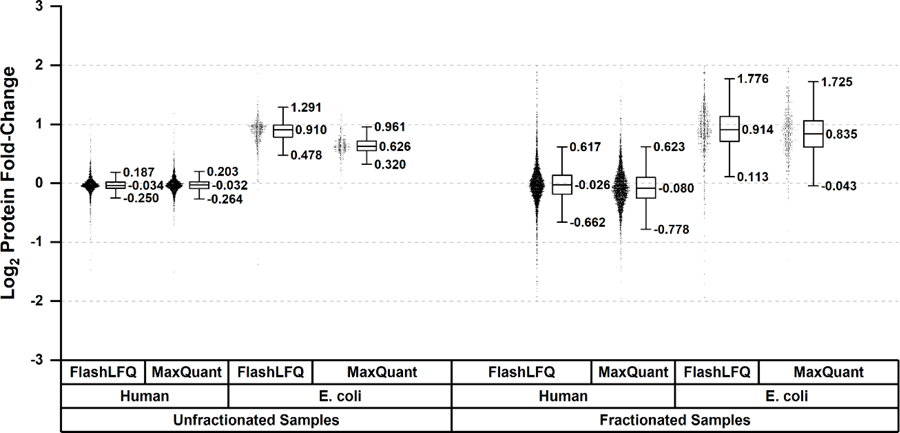
Protein fold-change measurements as measured by FlashLFQ and MaxQuant. E. coli proteins were doubling in abundance in both fractionated and unfractionated samples (a theoretical log2 fold-change of 1) and human proteins were not changing (a theoretical log2 fold-change of 0). Both software programs generally succeed at quantifying protein fold-changes accurately.
Evaluation of FlashLFQ’s false discovery rate estimation
Next, we evaluated FlashLFQ’s Bayesian hypothesis testing function. The result of this hypothesis test is a posterior error probability (PEP), which is the probability of a false-positive. The null hypothesis used in this test is a symmetric interval centered around zero that spans -T0 to T0 (e.g., −0.5 to 0.5). T0 is a combination of a subjective, user-defined value and an estimate of the uncertainty in the mean. The false discovery rate (FDR) of a set of proteins is an estimate of the proportion of false positives in the set, and is calculated by averaging the PEPs of the set. We evaluated this estimation by comparing it to the actual proportion of false positives in the set (the false discovery proportion, or FDP). In these two data sets, human proteins are not changing in abundance, and thus are quantitative false positives; E. coli proteins are doubling in abundance and are quantitative true positives. Figure 2 shows the FDP versus the FDR for both data sets. An ideal FDR estimation would perfectly correlate to the FDP; it would be a straight line along x=y.
Figure 2.
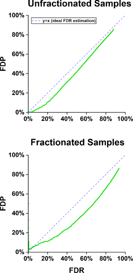
Accuracy of FlashLFQ’s estimated false discovery rate (FDR) using a fold-change cutoff of 0.1 for both data sets. The estimated FDR is a conservative estimate of the false-discovery proportion (FDP), which is calculated as the number of human proteins in the set divided by the number of proteins in the set. Proteins were ranked by PEP and then by number of peptides.
The FDR is a conservative estimate of the FDP in both data sets, though at the low end of the fractionated data set (FDR < 5%, Figure 2, bottom panel) there may be too few data points to draw reliable conclusions. One important note is that the width of the empirically-derived null hypothesis scales with intensity-dependent uncertainty in the data. The fractionated samples have a larger variance in their measurements than the unfractionated data, likely induced by fractionation. This results in a wider null hypothesis interval (a median value of 0.249 log2 units for the unfractionated samples, compared to 0.496 for the fractionated samples), and the bar to be classified as a true positive is higher compared to the unfractionated data.
Comparison of frequentist and Bayesian statistical analysis
Lastly, we compare FlashLFQ’s Bayesian FDR estimation with a frequentist (i.e., t-test centric) approach. Perseus[5] was used to determine the statistical significance of MaxQuant’s quantitative protein results. Five strategies using different filtering based on valid values and imputation were used; these strategies are described in Table 1. FDR was estimated at 5% via permutation. The “s0” parameter (fold-change cutoff) in Perseus was optimized such that the FDR accurately estimated the FDP, where possible. In the unfractionated data, FlashLFQ and all five MaxQuant/Perseus strategies adequately restricted false positives such that the FDP was close to the FDR (Figure 3, top panel); however, FlashLFQ showed improved sensitivity, detecting ~49% more truly changing E. coli proteins than the other approaches. In the fractionated samples, the FDR was adequately controlled by MaxQuant/Perseus strategies 1 and 5, but strategies 2, 3, and 4 showed many more false positives than were estimated (~21–31% FDP at estimated 5% FDR; Figure 3, bottom panel). Strategies 1 and 5, however, were not adequately sensitive; although they controlled false positives, no true positives were detected at all. By contrast, FlashLFQ detects 319 truly changing proteins, at an FDP of 5.6% compared to the estimated FDR of 5%.
We were curious if the difference in performance for FlashLFQ and MaxQuant/Perseus was primarily due to differences in the quantification algorithms or in the use of different statistical methods for FDR estimation. We thus analyzed MaxQuant’s peptide-level quantification results with our Bayesian hypothesis testing method. Bayesian analysis of MaxQuant’s results gave a ~17% improvement in the number of true positive proteins at 5% FDR compared to the frequentist statistical approach (Figure 4, top panel) in the unfractionated data set, though fewer true positives were detected compared to Bayesian analysis of FlashLFQ’s results. The same analysis performed on MaxQuant’s results for the fractionated data also showed a large increase in the number of true positives (Figure 4, bottom panel) and good FDR control. Thus, we conclude that MaxQuant and FlashLFQ both provide high-quality quantitative results, and the Bayesian method described here improves sensitivity compared to the frequentist approach while accurately estimating the FDP.
CONCLUSIONS
As evidenced by this manuscript and previous excellent work from several groups, we believe that both users and developers of statistical software should strongly consider Bayesian statistics to estimate effect sizes, perform hypothesis testing, and estimate false discovery rates. Perhaps the strongest case for Bayesian analysis is the flexibility and interpretability it offers in comparison to Student’s t-test. The t-test assumes that the underlying data are sampled from a normal distribution and calculates the probability of the test statistic under the assumption that the null hypothesis is true. By contrast, Bayesian analysis can use different distributions to model the data, test many competing custom hypotheses, and calculate the probability that each hypothesis is true given the data (relative to the other tested hypotheses).
One consideration of note is that the empirical null hypothesis strategy that we describe combines a subjective fold-change cutoff with an approximation of the background to determine the width of the null hypothesis. In these two benchmark data sets, the background is somewhat overestimated, and the FDR estimation is therefore quite conservative. Future work will focus on providing a more accurate estimate of the background, thus increasing sensitivity to detect truly changing proteins.
Lastly, one should consider that the most interesting data points may be peptides which have consistent outlier fold-change measurements. These may in fact be non-erroneous abundance change measurements from digestion products of differentially-regulated proteoforms[32]. Future work will include the determination of the statistical significance of these peptide changes relative to the inlier peptides to perhaps suggest or support proteoform-level quantitative changes. Additional possible improvements to FlashLFQ include quantification of top-down proteomics data, ANOVA-style multi-group hypothesis testing, and limit-of-detection estimation/imputation.
Supplementary Material
Supporting Information Table S2. Filtering, imputation, and fold-change cutoffs used in Perseus. (Enclosed in separate Microsoft Excel .xlsx file)
Supporting Information Table S1. TREAT FDR vs. FDP results for described data sets.
Supporting Information Figure S1. FDR vs. FDP for permutation and Benjamini-Hochberg multiple testing corrections calculated by Perseus.
Supporting Information Figure S2. FDR vs. FDP calculations from a hypothesis testing procedure conducted with a diffuse prior.
Supporting Information Figure S3. Fold-change estimation of E. coli proteins with a hypothesis testing prior.
Supporting Methods 1. FlashLFQ’s match-between-runs algorithm.
Supporting Methods 2. FlashLFQ’s intensity normalization algorithm.
Supporting Methods 3. Fractionated benchmark data set preparation.
Supporting Methods 4. Fractionated benchmark data set experimental design.
Supporting Methods 5. Description of data models and prior probability distributions.
Supporting Methods 6. Calculation of the prior for the mean in the hypothesis test.
Supporting Methods 7. Calculations to create the intensity-dependent prior for sigma.
ACKNOWLEDGMENTS
We thank the entire proteomics software development team of the Smith lab (Anthony J. Cesnik, Khairina Ibrahim, Lei Lu, Rachel M. Miller, Zach Rolfs, and Leah V. Schaffer), who contributed daily input and guidance to the improvement of FlashLFQ.
Funding Sources
This work was supported by grant R35GM126914 from the National Institute of General Medical Sciences. R.J.M. was supported by an NHGRI training grant to the Genomic Sciences Training Program 5T32HG002760.
ABBREVIATIONS
- FDR
false discovery rate
- FDP
false discovery proportion
- LC
liquid chromatography
- LFQ
label-free quantification
Footnotes
The authors declare no competing financial interest.
REFERENCES
- (1).Aebersold R; Mann M Mass Spectrometry-Based Proteomics. Nature 2003, 422 (6928), 198–207. [DOI] [PubMed] [Google Scholar]
- (2).Nesvizhskii AI; Keller A; Kolker E; Aebersold R A Statistical Model for Identifying Proteins by Tandem Mass Spectrometry. Anal. Chem 2003, 75 (17), 4646–4658. 10.1021/ac0341261. [DOI] [PubMed] [Google Scholar]
- (3).Yang X; Dondeti V; Dezube R; Maynard DM; Geer LY; Epstein J; Chen X; Markey SP; Kowalak JA DBParser: Web-Based Software for Shotgun Proteomic Data Analyses. J. Proteome Res 2004, 3 (5), 1002–1008. 10.1021/pr049920x. [DOI] [PubMed] [Google Scholar]
- (4).Cox J; Mann M MaxQuant Enables High Peptide Identification Rates, Individualized p.p.b.-Range Mass Accuracies and Proteome-Wide Protein Quantification. Nat. Biotechnol 2008, 26 (12), 1367–1372. 10.1038/nbt.1511. [DOI] [PubMed] [Google Scholar]
- (5).Tyanova S; Temu T; Sinitcyn P; Carlson A; Hein MY; Geiger T; Mann M; Cox J The Perseus Computational Platform for Comprehensive Analysis of (Prote)Omics Data. Nat. Methods 2016, 13 (9), 731–740. 10.1038/nmeth.3901. [DOI] [PubMed] [Google Scholar]
- (6).Argentini A; Goeminne LJE; Verheggen K; Hulstaert N; Staes A; Clement L; Martens L MoFF: A Robust and Automated Approach to Extract Peptide Ion Intensities. Nat. Methods 2016, 13 (12), 964–966. 10.1038/nmeth.4075. [DOI] [PubMed] [Google Scholar]
- (7).Wieczorek S; Combes F; Lazar C; Giai Gianetto Q; Gatto L; Dorffer A; Hesse A-M; Couté Y; Ferro M; Bruley C; et al. DAPAR & ProStaR: Software to Perform Statistical Analyses in Quantitative Discovery Proteomics. Bioinformatics 2017, 33 (1), 135–136. 10.1093/bioinformatics/btw580. [DOI] [PMC free article] [PubMed] [Google Scholar]
- (8).Choi M; Chang C-Y; Clough T; Broudy D; Killeen T; MacLean B; Vitek O MSstats: An R Package for Statistical Analysis of Quantitative Mass Spectrometry-Based Proteomic Experiments. Bioinformatics 2014, 30 (17), 2524–2526. 10.1093/bioinformatics/btu305. [DOI] [PubMed] [Google Scholar]
- (9).Suomi T; Corthals GL; Nevalainen OS; Elo LL Using Peptide-Level Proteomics Data for Detecting Differentially Expressed Proteins. J. Proteome Res 2015, 14 (11), 4564–4570. 10.1021/acs.jproteome.5b00363. [DOI] [PubMed] [Google Scholar]
- (10).Gutierrez M; Handy K; Smith R XNet: A Bayesian Approach to Extracted Ion Chromatogram Clustering for Precursor Mass Spectrometry Data. J. Proteome Res 2019, 18 (7), 2771–2778. 10.1021/acs.jproteome.9b00068. [DOI] [PubMed] [Google Scholar]
- (11).The M; Käll L Integrated Identification and Quantification Error Probabilities for Shotgun Proteomics. Mol. Cell. Proteomics 2019, 18 (3), 561–570. 10.1074/mcp.RA118.001018. [DOI] [PMC free article] [PubMed] [Google Scholar]
- (12).Välikangas T; Suomi T; Elo LL A Comprehensive Evaluation of Popular Proteomics Software Workflows for Label-Free Proteome Quantification and Imputation. Brief. Bioinform 2017. 10.1093/bib/bbx054. [DOI] [PMC free article] [PubMed] [Google Scholar]
- (13).Weisser H; Choudhary JS Targeted Feature Detection for Data-Dependent Shotgun Proteomics. J. Proteome Res 2017, 16 (8), 2964–2974. 10.1021/acs.jproteome.7b00248. [DOI] [PMC free article] [PubMed] [Google Scholar]
- (14).Zhang B; Pirmoradian M; Zubarev R; Käll L Covariation of Peptide Abundances Accurately Reflects Protein Concentration Differences. Mol. Cell. Proteomics 2017, 16 (5), 936–948. 10.1074/mcp.O117.067728. [DOI] [PMC free article] [PubMed] [Google Scholar]
- (15).McCarthy DJ; Smyth GK Testing Significance Relative to a Fold-Change Threshold Is a TREAT. Bioinformatics 2009, 25 (6), 765–771. 10.1093/bioinformatics/btp053. [DOI] [PMC free article] [PubMed] [Google Scholar]
- (16).Millikin RJ; Solntsev SK; Shortreed MR; Smith LM Ultrafast Peptide Label-Free Quantification with FlashLFQ. J. Proteome Res 2018, 17 (1), 386–391. 10.1021/acs.jproteome.7b00608. [DOI] [PMC free article] [PubMed] [Google Scholar]
- (17).Student. The Probable Error of a Mean. Biometrika 1908, 6 (1), 1–25. [Google Scholar]
- (18).Tusher VG; Tibshirani R; Chu G Significance Analysis of Microarrays Applied to the Ionizing Radiation Response. Proc. Natl. Acad. Sci 2001, 98 (9), 5116–5121. 10.1073/pnas.091062498. [DOI] [PMC free article] [PubMed] [Google Scholar]
- (19).Kruschke JK Bayesian Estimation Supersedes the t Test. J. Exp. Psychol. Gen 2013, 142 (2), 573–603. 10.1037/a0029146. [DOI] [PubMed] [Google Scholar]
- (20).Wasserstein RL; Lazar NA The ASA Statement on p -Values: Context, Process, and Purpose. Am. Stat 2016, 70 (2), 129–133. 10.1080/00031305.2016.1154108. [DOI] [Google Scholar]
- (21).Koopmans F; Cornelisse LN; Heskes T; Dijkstra TMH Empirical Bayesian Random Censoring Threshold Model Improves Detection of Differentially Abundant Proteins. J. Proteome Res 2014, 13 (9), 3871–3880. 10.1021/pr500171u. [DOI] [PubMed] [Google Scholar]
- (22).Peshkin L; Gupta M; Ryazanova L; Wühr M Bayesian Confidence Intervals for Multiplexed Proteomics Integrate Ion-Statistics with Peptide Quantification Concordance. Mol. Cell. Proteomics 2019, 18 (10), 2108–2120. 10.1074/mcp.TIR119.001317. [DOI] [PMC free article] [PubMed] [Google Scholar]
- (23).Bernoulli J Ars Conjectandi; Impensis Thurnisiorum, fratrum, 1713.
- (24).Keynes JM Chapter IV: The Principle of Indifference In A Treatise on Probability; MacMillan and Co., 1921; pp 44–70. [Google Scholar]
- (25).Metropolis N; Rosenbluth AW; Rosenbluth MN; Teller AH; Teller E Equation of State Calculations by Fast Computing Machines. J. Chem. Phys 1953, 21 (6), 1087–1092. [Google Scholar]
- (26).Roberts GO; Rosenthal JS Examples of Adaptive MCMC. J. Comput. Graph. Stat 2009, 18 (2), 349–367. 10.1198/jcgs.2009.06134. [DOI] [Google Scholar]
- (27).Morey RD; Rouder JN Bayes Factor Approaches for Testing Interval Null Hypotheses. Psychol. Methods 2011, 16 (4), 406–419. 10.1037/a0024377. [DOI] [PubMed] [Google Scholar]
- (28).Wen X Robust Bayesian FDR Control Using Bayes Factors, with Applications to Multi-Tissue EQTL Discovery. Stat. Biosci 2017, 9, 28–49. 10.1007/s12561-016-9153-0. [DOI] [Google Scholar]
- (29).Rudmin JW Calculating the Exact Pooled Variance. ArXiv Prepr 10071012 2010, 1–4.
- (30).Shen X; Shen S; Li J; Hu Q; Nie L; Tu C; Wang X; Orsburn B; Wang J; Qu J An IonStar Experimental Strategy for MS1 Ion Current-Based Quantification Using Ultrahigh-Field Orbitrap: Reproducible, In-Depth, and Accurate Protein Measurement in Large Cohorts. J. Proteome Res 2017, 16 (7), 2445–2456. 10.1021/acs.jproteome.7b00061. [DOI] [PMC free article] [PubMed] [Google Scholar]
- (31).Perez-Riverol Y; Csordas A; Bai J; Bernal-Llinares M; Hewapathirana S; Kundu DJ; Inuganti A; Griss J; Mayer G; Eisenacher M; et al. The PRIDE Database and Related Tools and Resources in 2019: Improving Support for Quantification Data. Nucleic Acids Res 2019, 47 (D1), D442–D450. 10.1093/nar/gky1106. [DOI] [PMC free article] [PubMed] [Google Scholar]
- (32).Smith LM; Kelleher NL; The Consortium for Top Down Proteomics. Proteoform: A Single Term Describing Protein Complexity. Nat. Methods 2013, 10 (3), 186–187. 10.1038/nmeth.2369. [DOI] [PMC free article] [PubMed] [Google Scholar]
Associated Data
This section collects any data citations, data availability statements, or supplementary materials included in this article.
Supplementary Materials
Supporting Information Table S2. Filtering, imputation, and fold-change cutoffs used in Perseus. (Enclosed in separate Microsoft Excel .xlsx file)
Supporting Information Table S1. TREAT FDR vs. FDP results for described data sets.
Supporting Information Figure S1. FDR vs. FDP for permutation and Benjamini-Hochberg multiple testing corrections calculated by Perseus.
Supporting Information Figure S2. FDR vs. FDP calculations from a hypothesis testing procedure conducted with a diffuse prior.
Supporting Information Figure S3. Fold-change estimation of E. coli proteins with a hypothesis testing prior.
Supporting Methods 1. FlashLFQ’s match-between-runs algorithm.
Supporting Methods 2. FlashLFQ’s intensity normalization algorithm.
Supporting Methods 3. Fractionated benchmark data set preparation.
Supporting Methods 4. Fractionated benchmark data set experimental design.
Supporting Methods 5. Description of data models and prior probability distributions.
Supporting Methods 6. Calculation of the prior for the mean in the hypothesis test.
Supporting Methods 7. Calculations to create the intensity-dependent prior for sigma.