

Abstract
Understanding complex tissues requires single-cell deconstruction of gene regulation with precision and scale. Here, we assess the performance of a massively parallel droplet-based method for mapping transposase-accessible chromatin in single cells using sequencing (scATAC-seq). We apply scATAC-seq to obtain chromatin profiles of more than 200,000 single cells in human blood and basal cell carcinoma. In blood, application of scATAC-seq enables marker-free identification of cell type-specific cis- and trans-regulatory elements, mapping of disease-associated enhancer activity and reconstruction of trajectories of cellular differentiation. In basal cell carcinoma, application of scATAC-seq reveals regulatory networks in malignant, stromal and immune cells in the tumor microenvironment. Analysis of scATAC-seq profiles from serial tumor biopsies before and after programmed cell death protein 1 blockade identifies chromatin regulators of therapy-responsive T cell subsets and reveals a shared regulatory program that governs intratumoral CD8+ T cell exhaustion and CD4+ T follicular helper cell development. We anticipate that scATAC-seq will enable the unbiased discovery of gene regulatory factors across diverse biological systems.
Cell type-specific gene expression in eukaryotic cells is regulated by millions of cis-acting DNA elements (for example, enhancers and promoters) and thousands of trans-acting factors (for example, transcription factors (TFs))1. We previously developed the assay for transposase-accessible chromatin using sequencing (ATAC-seq), which identifies active DNA regulatory elements by transposition of sequencing adapters into accessible chromatin with the hyperactive transposase Tn5 (ref. 2). This method can reveal several layers of gene regulation in a single assay, including genome-wide identification of cis-elements, inference of TF binding and activity, and nucleosome positions2–4. ATAC-seq is applicable to low-cell-number samples5, and even single cells6,7, which has enabled epigenomic profiling of primary samples with newfound precision. To date, scATAC-seq has been used to map cell-to-cell variability and rare cell phenotypes, including in healthy and malignant immune cells8–12. However, the widespread adoption of this technique has been hindered by the difficulty and cost of performing the assay at scale.
Here, we used a commercial system to perform scATAC-seq in nanoliter-sized droplets, which enables the generation of high-quality single-cell chromatin accessibility profiles at massive scale. To systematically benchmark the performance of this method, we analyzed primary cells in two biological contexts. First, we mapped the single-cell chromatin accessibility landscape of blood formation in bone marrow and blood samples from healthy humans, which revealed chromatin states of progenitor cells and the regulatory trajectories of their differentiation into effector cell types. Second, we performed scATAC-seq in primary tumor biopsies from patients with basal cell carcinoma (BCC) receiving anti-programmed cell death protein 1 (PD-1) immunotherapy (PD-1 blockade). Single-cell deconvolution of the tumor microenvironment (TME) revealed distinct types of immune, stromal and malignant cells, and analysis of intratumoral T cells identified regulators of therapy-responsive T cell subtypes, including CD8+ exhausted (TEx) and CD4+ T follicular helper (Tfh) cells. Altogether, we report scATAC-seq profiles of over 200,000 cells, demonstrating that this platform enables the unbiased discovery of cell types and regulatory DNA elements across diverse biological systems.
Results
Droplet-based platform for scATAC-seq.
We performed scATAC-seq in droplets using the Chromium platform (10x Genomics) previously employed to measure single-cell transcriptomes13,14 (Fig. 1a and Supplementary Fig. 1a). In this approach, nuclei are first isolated from a single-cell suspension and transposed in bulk with the transposase Tn5. Transposed nuclei are then loaded onto a microfluidic chip for gel bead in emulsion (GEM) generation. Each gel bead is functionalized with single-stranded barcoded oligonucleotides that consist of a 29-base pair (bp) sequencing adapter, a 16-bp barcode selected from ~750,000 designed sequences to index GEMs and the first 14 bp of read 1N, which serves as the priming sequence in the linear amplification reaction to incorporate barcodes to transposed DNA (Supplementary Fig. 1a and Supplementary Table 1). Approximately 100,000 GEMs are formed in each channel, resulting in the encapsulation of tens of thousands of nuclei in GEMs per experiment. After GEM generation, gel beads are dissolved and the oligonucleotides are released for linear amplification of transposed DNA. Finally, the emulsion is broken, and barcoded DNA is pooled for PCR amplification to generate indexed libraries for high-throughput sequencing.
Fig. 1 |. Massively parallel scATAC-seq in droplets.
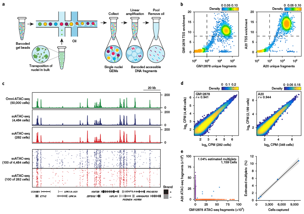
a, Schematic of scATAC-seq in droplets. b, ATAC-seq data quality control filters in human (GM12878) and mouse (A20) B cells at 5,000 cell loading. Shown are the number of unique ATAC-seq nuclear fragments in each single cell (each dot) compared with TSS enrichment of all fragments in that cell. Dashed lines represent the filters for high-quality single-cell data (1,000 unique nuclear fragments and TSS score greater than or equal to 8). Density is given in arbitrary units. Data are representative of four independent experiments. c, Genome tracks showing the comparison of aggregate scATAC-seq profiles with bulk Omni-ATAC-seq profiles from GM12878 B lymphoblasts (top panel). scATAC-seq profiles were obtained from 2 independent mixing experiments, in which either 4,484 (from 10,000 cell loading) or 282 (from 500 cell loading) cells were assayed, as indicated. The bottom panel shows accessibility profiles of 100 random single GM12878 cells from each experiment. Each pixel represents a 100-bp region. d, One-to-one plots of log-normalized reads in ATAC-seq peaks in aggregate scATAC-seq profiles (n = 100,000 ATAC-seq peaks, Pearson correlation). Aggregate profiles in GM12878 (left) and A20 (right) cells are derived from two individual mixing experiments as in b, in which the indicated numbers of cells were assayed. ATAC-seq peaks were identified in Omni-ATAC-seq profiles from 50,000 cells5. e, Human (GM12878)/mouse (A20) cell mixing experiment showing proportion of single-cell libraries with both mouse and human ATAC-seq fragments (left). The right panel shows proportion of mouse/human multiplets detected when cell-loading concentration was varied (n = 4 biologically independent experiments). The center line indicates linear fit, and shaded lines indicate 95% confidence interval.
To assess the performance of this method, we generated scATAC-seq libraries from species-mixing experiments, in which we pooled human (GM12878) and mouse (A20) B cell nuclei. Libraries were sequenced and processed to de-multiplex reads, assign cell barcodes, align fragments to the human and mouse reference genomes and deduplicate fragments generated by PCR (Cell Ranger ATAC; see Methods). We filtered scATAC-seq data using previously described cut-offs of 1,000 unique nuclear fragments per cell and a transcription start site (TSS) enrichment score of 8 to exclude low-quality cells15. Cells passing filter yielded on average 27.8 × 10³ unique fragments mapping to the nuclear genome, and approximately 38.1% of Tn5 insertions were within peaks present in aggregated profiles from all cells, comparable to published high-quality ATAC-seq profiles (Fig. 1b, c and Supplementary Fig. 1b)6,10,15. scATAC-seq profiles exhibited fragment size periodicity and a high enrichment of fragments at TSSs, and aggregate profiles from multiple independent experiments were highly correlated (Fig. 1d and Supplementary Fig. 1c). Finally, we observed a low rate of estimated multiplets (12 of 1,159 cells, ~1%; Fig. 1e). A cell titration experiment with four cell-loading concentrations showed a linear relationship between the observed multiplet rate and the number of recovered cells (Fig. 1e).
Rare cell detection and performance in archival samples.
We subsampled scATAC-seq data in silico, which showed that aggregate profiles from ~200 cells could achieve the confident discovery of ~80% of ATAC-seq peaks from total profiles and a Pearson correlation of r ~ 0.9 for all reads in peaks (Supplementary Fig. 1d,e). Using this information, we devised an analysis workflow for peak calling and clustering (Supplementary Fig. 1f and see Methods). Single-cell libraries were first processed with Cell Ranger and filtered, and then we performed an ‘initial’ clustering by partitioning the genome into 2.5-kb windows and counting Tn5 insertions in each window, as described previously7,9. We then performed latent semantic indexing (LSI) and clustered cells using shared nearest neighbor (SNN) clustering (Seurat16) with the top 20,000 accessible windows, requiring that each cluster contain at least 200 cells. These ‘initial’ clusters were used to identify ATAC-seq peaks (using MACS2 (ref. 17)) and to generate a merged peak set. Finally, a cell-by-peak counts matrix was created and used for ‘final’ clustering and downstream analysis, in which each cluster could contain any number of cells.
We tested this analysis approach with two quality-control experiments. First, we generated synthetic cell mixtures, in which human monocytes and T cells were isolated from peripheral blood mononuclear cells (PBMCs) and mixed in various ratios (Supplementary Fig. 2a,b and Supplementary Table 2). We then performed scATAC-seq and attempted to resolve each population in an unsupervised analysis. As expected, analysis of 50:50 mixtures identified 2 distinct populations of cells, which demonstrated accessibility of open chromatin regions linked either to monocyte-specific genes (that is, CD14, CSF1R, TREML4) or to T cell-specific genes (that is, CD3E, CD4, CD8A; Supplementary Fig. 2a). Importantly, this analysis could also resolve populations that represented either 1 of 100 or 1 of 1,000 total cells (Supplementary Fig. 2b and Supplementary Table 3). Second, we compared the performance of scATAC-seq in fresh versus frozen PBMCs (Supplementary Fig. 2c–f). We isolated nuclei from either fresh PBMCs, viably frozen PBMCs or viably frozen PBMCs sorted for live cells, and performed scATAC-seq. We confirmed that scATAC-seq profiles passing filter yielded approximately the same quantity and quality of data, regardless of sample origin (Supplementary Fig. 2c)11. Namely, aggregate profiles from fresh and frozen cells were highly correlated, frozen samples recapitulated the majority of ATAC-seq peaks discovered in fresh samples (area under the curve, 0.809) and scATAC-seq profiles across batches clustered together (Supplementary Fig. 2d–g).
Single-cell chromatin landscape of human hematopoiesis.
To demonstrate this method in primary samples, we performed experiments in human immune cells (Fig. 2a). We generated scATAC-seq libraries from peripheral blood and bone marrow cells from 16 healthy individuals and sampled cells in an unbiased fashion, or after enrichment for surface phenotypes (Supplementary Fig. 3a and Supplementary Table 4). In total, we generated scATAC-seq profiles from 61,806 cells, which yielded on average 15.6 × 10³ unique fragments mapping to the nuclear genome, and approximately 40.5% of Tn5 insertions were within aggregate ATAC-seq peaks (Supplementary Fig. 3b,c). The quality of scATAC-seq profiles was highly uniform across individuals, samples and cell types, and on a par with scATAC-seq profiles generated with other technologies (Supplementary Fig. 3d–f)11,12. We identified 31 scATAC-seq clusters and visualized single-cell profiles with uniform manifold approximation and projection (UMAP)18. We classified each cluster using three parallel approaches: (1) chromatin accessibility of cis-elements (ATAC-seq peaks); (2) gene activity scores, computed from the accessibility of several enhancers linked to a single gene promoter19; and (3) TF activity, computed from the accessibility of TF binding sites genome-wide in each single cell4. All three approaches represent a ‘bottom-up’ analysis of scATAC-seq data and do not require previous knowledge from RNA sequencing or bulk ATAC-seq profiles.
Fig. 2 |. Single-cell chromatin accessibility of human hematopoiesis.

a, Schematic of progenitor and end-stage cell types in human hematopoiesis. MPP, multipotent progenitor; LMPP, lymphoid-primed multipotent progenitor; CLP, common lymphoid progenitor; MEP, megakaryocyte-erythroid progenitor; BMP, basophil-mast cell progenitor; N CD4, naïve CD4 T cell; N CD8, naïve CD8 T cell; M CD4, memory CD4 T cell; CD8 CM, CD8 central memory T cell; CD8 EM, CD8 effector memory T cell; Imm NK, immature natural killer cell; Mat NK, mature natural killer cell; Neut, neutrophil; Meg, megakaryocyte; Ery, erythrocyte; Eos, eosinophil; Baso, basophil. Lightly shaded cells were not sampled in the current study. b, UMAP projection of 63,882 scATAC-seq profiles of bone marrow and peripheral blood immune cell types. Dots represent individual cells, and colors indicate cluster identity (labeled on the right). Bar plot indicates the number of scATAC-seq profiles in each cluster of cells. Cells include those generated in this study (61,806) and cells from a previous study11 (2,076). c, Heatmap of Z-scores of 116,713 cis-regulatory elements in scATAC-seq clusters derived from b. Gene labels indicate the nearest gene to each regulatory element. d, Single-cell chromatin accessibility in the IRF8 locus. Each box shows scATAC-seq profiles from 100 representative single cells from each cluster. Each pixel represents a 200-bp region. The top genome track shows the aggregate accessibility profile from all cells combined. e, UMAP projection colored by log-normalized gene scores demonstrating the accessibility of cis-regulatory elements linked (computed from linked accessibility of distal peaks to peaks at gene promoters using Cicero) to the indicated gene. Gene scores are calculated as log2(GA*1000000 + 1), which we refer to as log2(GA + 1). For example, the top left plot demonstrates the accessibility score for cis-elements linked to the promoter of the hematopoietic progenitor gene CD34. f, Example TF footprints of GATA2 and EBF1 with motifs in the indicated scATAC-seq clusters. The Tn5 insertion bias track is shown below. g, Heatmap representation of ATAC-seq chromVAR bias-corrected deviations in the 250 most variable TFs across all scATAC-seq clusters. Single-cell cluster identities are indicated at the top of the plot. h, UMAP projection of scATAC-seq profiles colored by chromVAR TF motif bias-corrected deviations for the indicated factors.
Using the first approach, we identified 571,400 cis-elements across all clusters, and approximately 20.4% of elements (116,713) exhibited cell type-specific accessibility (mean, 6,208 peaks per cluster; false discovery rate (FDR) < 0.01). Annotation of cell types using neighboring genes to cluster-specific cis-elements demonstrated that scATAC-seq profiles spanned the continuum from early progenitors to end-stage cell types (Fig. 2b, c and Supplementary Fig. 4a). For example, clusters 2–4 demonstrated accessibility at cis-elements neighboring myeloid progenitor genes, including GATA1, TAL1 and SPI1, while clusters 14–16 demonstrated accessibility at cis-elements neighboring B cell genes, including CD19, EBF1 and LYN (Fig. 2c). Clustering of scATAC-seq profiles could identify known cell type distinctions, such as CD4+ and CD8+ T cells, the presence of phenotypically distinct cell subsets, such as regulatory CD4+ T cells (Tregs), and even relatively rare cell types, such as basophils (Fig. 2b,c). Moreover, scATAC-seq analysis identified cell type-specific cis-elements even within a single gene locus. For example, we observed unique accessibility of the +85 kb and +87 kb enhancers in the IRF8 locus in myeloid cells, and of the +54 kb and +56 kb enhancers in plasmacytoid dendritic cells (pDCs), while the +37 kb enhancer was accessible in nearly all immune lineages (Fig. 2d). These findings are in line with previously identified Irf8 super-enhancers in dendritic cells (DCs)20 and may inform the cellular impact of disease variants in this locus21.
Although cis-element analysis can be informative, this measurement is sparse in single cells, as it is limited by the DNA copy number. Therefore, in the second analysis approach, we used gene activity scores (referred to as ‘gene scores’), which represent the aggregate accessibility of several enhancers linked to a single gene promoter19. We first identified all enhancer–promoter (E-P) connections genome-wide with Cicero, an algorithm that links DNA elements based on co-accessibility in scATAC-seq data. This method identified 149,309 E-P connections across all scATAC-seq clusters, with a median of 6 enhancers linked to each promoter (Methods). We independently validated E-P connections using two orthogonal datasets. First, we compared E-P connections to chromosome conformation signal obtained from H3K27ac HiChIP in T cells22 and found significant enrichment for HiChIP enhancer interaction signal in linked contacts (Supplementary Fig. 4b). Second, we compared E-P connections with expression quantitative trait loci (eQTLs23) and found enrichment of eQTLs in linked contacts, particularly when eQTLs were also identified in immune cells (Supplementary Fig. 4c). We next projected gene scores for immune lineage-defining genes onto scATAC-seq profiles, which supported cis-element-defined cluster identities (Fig. 2e). For example, the CD34 gene score identified hematopoietic progenitors, the CD14 gene score identified monocytes and classical dendritic cells (cDCs) and the CD20 gene score identified B cells (Fig. 2e and Supplementary Fig. 4d,e). Again, this analysis identified immune cell subsets, for example demonstrating high FOXP3 gene scores in Tregs, and rare cell types, for example demonstrating high IL13 gene scores in basophils (Supplementary Fig. 4e). Across all single cells, we identified 5,977 gene scores that exhibited cluster-specific activity, reflecting markers for each cell type (Supplementary Fig. 4d).
Finally, in the third analysis approach, we measured chromatin accessibility at cis-elements sharing a TF binding motif using chromVAR4. To validate this method, we analyzed accessibility changes in binding sites for known cell type-specific TFs (referred to as TF deviation scores). Indeed, TF deviation scores for GATA2, a lineage-determining factor for megakaryocyte, erythrocyte and basophil lineages24, were increased in megakaryocyte-erythroid progenitors, basophils and common myeloid progenitors (CMPs; Fig. 2f). Similarly, the TF deviation scores for EBF1, a lineage-determining factor for B cells25, were increased in naïve, memory and plasma B cells, as well as in early B cell progenitors (Fig. 2f). Since DNA bound by TFs is protected from transposition by Tn5, visualization of each TF profile showed local chromatin accessibility changes surrounding the binding ‘footprint’ (Fig. 2f and Supplementary Fig. 5a). Deviation scores for all TF motifs revealed shared and unique regulatory programs across immune cell types (Fig. 2g,h and Supplementary Fig. 5b). For example, cDCs and B cells shared activity of BCL11A, SPI1 and IRF factor motifs, but demonstrated unique activity of CEBP factors and EBF1, respectively (Fig. 2g, h). Similarly, TBX21 and EOMES were active in natural killer (NK) and T cell populations; however, only T cells showed activity of the T cell lineage-determining factor TCF7 (Fig. 2g,h)26.
We also grouped cis-elements according to the presence of causal risk variants associated with 21 autoimmune diseases and 18 non-immune diseases21 and generated a feature set of variant-containing ATAC-seq peaks and their co-accessible elements for each disease (referred to as ‘variant-enhancers’; Supplementary Fig. 5c). We then measured chromatin accessibility in variant-enhancers to nominate causal cell types for each disease (chromVAR; Supplementary Fig. 5c,d). Several diseases, such as celiac disease, type 1 diabetes, Crohn’s disease and juvenile arthritis, showed high accessibility of variant-enhancers in T-cell populations (Supplementary Fig. 5d)21. Other diseases, such as Kawasaki disease, multiple sclerosis and systemic lupus erythematosus, showed high accessibility of variant-enhancers in B cells—either specifically or in addition to accessibility in T cells (Supplementary Fig. 5d)21. scATAC-seq data also enabled the discovery of patterns in additional cell types. For example, variant-enhancers associated with systemic sclerosis showed high accessibility in NK cells and pDCs, and variant-enhancers associated with ulcerative colitis showed high accessibility in cDCs and monocytes, consistent with the roles of these cell types in murine models of each disease27,28. Additional diseases with high variant-enhancer signals in myeloid cells included metabolic traits and diseases, such as fasting glucose, high-density lipoprotein cholesterol levels and type 2 diabetes, suggesting regulatory roles for myeloid cells in these processes as well. We confirmed associations of disease variants with cell type-specific enhancers using H3K27ac HiChIP (Supplementary Fig. 5e).
Regulatory trajectories of immune cell lineages.
We used scATAC-seq to reconstruct cellular developmental trajectories in an unbiased manner. As a test case, we reconstructed the lineage trajectory of plasma B cell differentiation, since: (1) the developmental program occurs in the bone marrow and blood and thus ought to be captured in our dataset, and (2) the regulatory mechanisms of this process are well-defined for comparison (Fig. 3a). To achieve this, we used a nearest-neighbor approach on existing cluster definitions (Fig. 3a, b). We started with the plasma B cell cluster (cluster 16) and attempted to return to the hematopoietic stem cell (HSC) cluster (cluster 1) by sequentially selecting precursor cells with the most epigenetic similarity (Euclidean distances of ATAC-seq profiles; see Methods). Indeed, this reverse reconstruction process identified the well-established cellular trajectory of plasma B cell development as the most significant among all tested trajectories (P < 0.0002; 5,000 permutations). Finally, we generated an ordering of single cells (referred to as ‘pseudotime’) along this trajectory by computing a vector across lineage clusters and aligning each cell to the vector in the UMAP projection (Fig. 3c). An analysis of ~10,000 cis-elements with dynamic accessibility patterns across the trajectory revealed cis-elements near known regulators of every stage of B cell development (Fig. 3d). For example, cis-elements that were accessible early in the trajectory included enhancers for EBF1, RUNX1, IL7R, RAG2 and MEF2C, factors that are critical for B cell lineage specification (Fig. 3d)25,29,30. Cis-elements that were accessible late in the trajectory included elements proximal to PRDM1, a critical TF for plasma cell fate, and the plasma cell-specific marker SDC1 (CD138). Since TF deviation scores can reflect the activity of many TFs with similar DNA-binding motifs, we integrated chromVAR deviations with gene scores to prune the data for relevant TFs within a motif family (Fig. 3e). Indeed, this method accurately identified TFs that are critical for B cell differentiation and resolved the timing of TF activity (Fig. 3e). For example, MEF2C activity was observed early in B cell development, consistent with its role in lymphoid fate specification30, followed by the sequential activity of EBF1, PAX5 and IRF4, recapitulating the known order of their functions in pro-B cells, pre-B cells and naïve B cells, respectively (Fig. 3f)25.
Fig. 3 |. Epigenomic differentiation trajectories of human immune cell types.
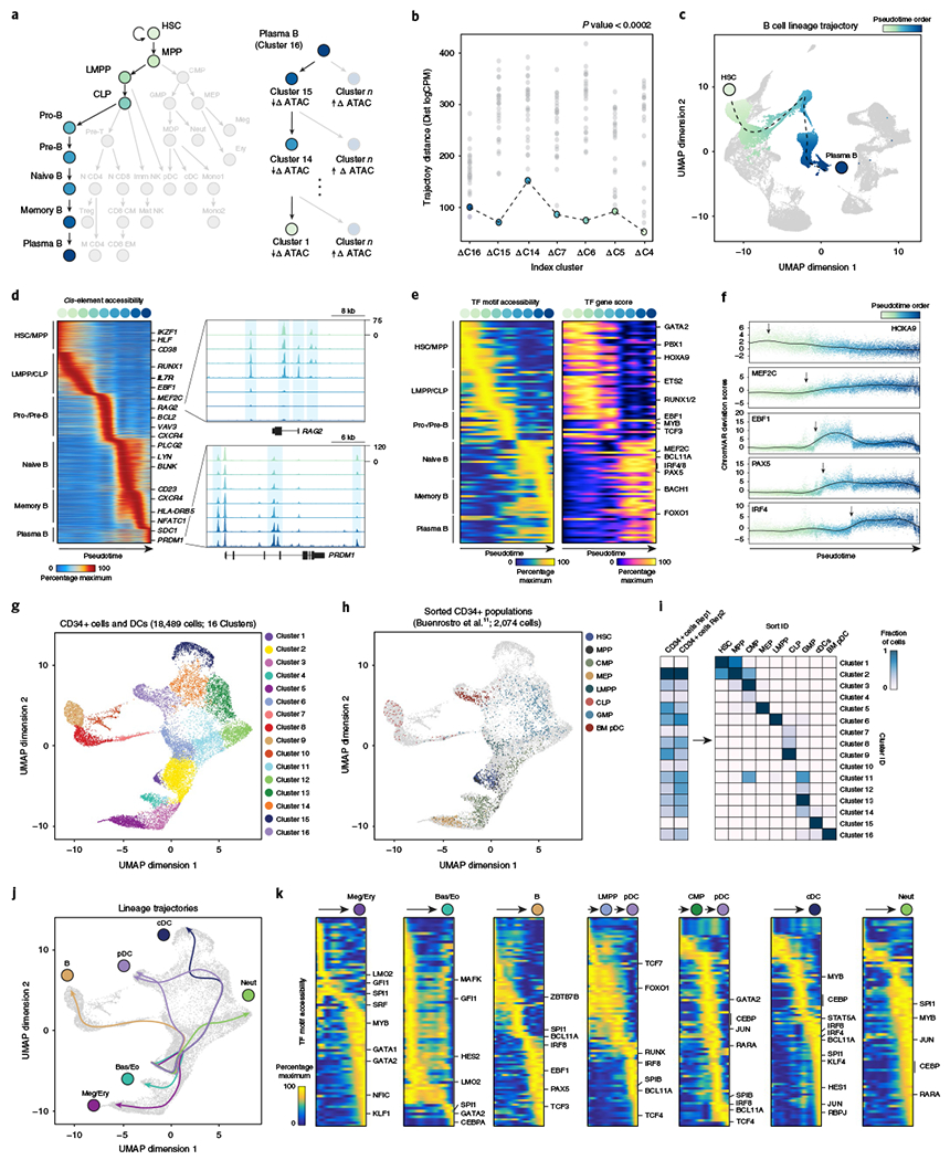
a, Differentiation trajectory of HSCs to terminal plasma B cells (left). Reverse reconstruction of B cell differentiation trajectory using scATAC-seq profiles (right; see Methods). Differences between the aggregate plasma B cell scATAC-seq profile and all other clusters are calculated. Trajectory is tested against a nearest-neighbor approach; the cluster with the most similarity (lowest trajectory distance) to the cluster of interest is identified as the immediate precursor cluster. b, Trajectory distance calculations for the terminal plasma B cell cluster (cluster 16). Dots represent comparisons between the cluster of interest (labeled at the bottom) and every cluster not previously identified. P < 0.0002 calculated as one-sided empirical P value from 5,000 random simulations of trajectory ordering. c, Pseudotime representation of plasma B cell differentiation from HSCs. The dashed line represents a double-spline fitted trajectory across pseudotime. d, Pseudotime heatmap ordering of the top 10,000 variable cis-regulatory elements across B cell differentiation (left). Zoom-in genome tracks show representation of behavior of cis-elements accessible early (top) and late in B cell differentiation (bottom). e, Pseudotime heatmap ordering of chromVAR TF motif bias-corrected deviations across B cell differentiation (left). TF motifs are filtered for genes that are highly active (defined as the average percentile between total gene score and variability) that also demonstrate similarly dynamic gene scores across differentiation (R > 0.35 and FDR < 0.001 across 1,000 incremental groups). Heatmap of TF gene scores is shown on the right. f, chromVAR bias-corrected deviation scores for the indicated TFs across B cell pseudotime. Each dot represents the deviation score in an individual pseudotime-ordered scATAC-seq profile. The line represents the smoothed fit across pseudotime and chromVAR deviation scores. g, Subclustering UMAP projection of 18,489 CD34+ bone marrow progenitors and DCs (cells within clusters 1–6 and 8–11 from full hematopoiesis). scATAC-seq profiles are colored by cluster identity, as labeled on the right. h, UMAP projection of progenitor populations; highlighted are the sorted progenitor populations from Buenrostro et al.11. Grayed out are the cells assayed in this study. CMPs (green dots) were sorted as lineage−CD34+CD38+CD10−CD45RA−CD123mid, and GMPs (light blue dots) were sorted as lineage−CD34+CD38+CD10−CD45RA+CD123mid. i, Confusion matrix of sorted progenitor populations showing the proportion of each population in clusters defined in g. j, Lineage trajectories for the indicated cell types, calculated as described in a. Lines represent double-spline fitted trajectories across pseudotime. k, Pseudotime heatmap ordering of chromVAR TF motif bias-corrected deviations in the indicated lineage trajectory. TF motifs are filtered for genes as described in e.
We applied trajectory analysis to early stages of hematopoiesis to identify regulators of myeloid fate decisions, particularly of DCs. We re-clustered 16,415 progenitor and DC scATAC-seq profiles, and 2,074 profiles of surface marker-defined progenitors generated in a previous study (Fig. 3g)11. We identified 16 subclusters, and projection of sorted scATAC-seq profiles onto de novo-defined clusters revealed significant heterogeneity in marker-defined states (Fig. 3h,i). Globally, immune lineages appeared to diverge early via three distinct branches to: (1) megakaryocyte/erythroid (Meg/E) and basophil/eosinophil (Bas/Eo) fates, (2) lymphoid fates or (3) neutrophil/monocyte/DC fates. However, sorted progenitors did not always occupy a single de novo-defined regulatory state. For example, CMPs were present in 4 de novo-defined clusters, including in committed pathways leading to neutrophil/monocyte/DC fates (clusters 2 and 11), Meg/E fates (clusters 4 and 5) or Baso/Eo fates (clusters 3 and 4; Fig. 3h,i). Similarly, granulocyte-macrophage progenitors (GMPs) were present in 4 clusters downstream of the CMP (clusters 11–14), including those leading to neutrophil differentiation, as well as clusters leading to cDC and pDC fates (Fig. 3h,i).
Analysis of TF activity revealed shared and unique TF programs across myeloid trajectories (Fig. 3j). For example, Meg/E and Bas/Eo progenitors shared accessibility at GATA2 motifs, but Bas/Eo commitment was characterized by SPI1 (PU.1) and CEBPA motif activity, while Meg/E commitment was characterized by MYB, GATA1 and KLF1 motif activity (Fig. 3k)31,32. Similarly, neutrophil progenitors shared accessibility at SPI1 motifs with Bas/Eo progenitors, but neutrophil commitment was accompanied by additional activity of AP-1, CEBP and RARA motifs (Fig. 3k). Finally, the analysis of trajectories toward DC fates revealed three pathways. The cDC pathway transitioned through CMP and GMP clusters, and then to cluster 13 (monocyte-dendritic cell progenitor; MDP) and cluster 14 (common dendritic progenitor; CDP), before terminal cDC differentiation. This trajectory showed accessibility at IRF8, IRF4, BCL11A, SPI1, AP-1 and RBPJ motifs, consistent with roles of each factor in DC differentiation33. IRF8, BCL11A and SPI1 motifs exhibited accessibility early in CDPs, while AP-1 and RBPJ factors exhibited late accessibility (Fig. 3k). For pDCs, two possible trajectories were observed, supporting reports that this lineage can arise from both myeloid- and lymphoid-committed progenitors34–36. One pDC trajectory transitioned directly from lymphoid-primed multipotent progenitors to differentiated pDCs, while a second trajectory traversed CMP, GMP, MDP and CDP stages before pDC differentiation (Fig. 3k). Each pathway relied on the same regulatory program, which included RUNX, IRF8, SPIB, BCL11A and TCF4 factors33. Moreover, we did not observe significant epigenomic heterogeneity within terminal pDCs, suggesting that divergent cellular trajectories can achieve identical cell states through common regulatory programs.
Single-cell chromatin landscape of intratumoral immunity.
BCC is the most common cancer in humans worldwide, and recent studies demonstrated that patients with advanced BCC can obtain clinical benefit from immunotherapies that block the T cell inhibitory receptor PD-1 (ref. 37). However, as in many other cancers, PD-1 blockade is clinically ineffective in more than half of patients with BCC37,38. Thus, our goal was to use scATAC-seq to identify cell types that were responsive to therapy and the regulatory mechanisms controlling their activity. In addition, these experiments demonstrated the feasibility of applying scATAC-seq to sparse samples from clinical biopsies. We performed scATAC-seq on site-matched serial tumor biopsies pre- and post-PD-1 blockade (pembrolizumab) from five patients, plus post-therapy biopsies from two additional patients (Fig. 4a and Supplementary Table 5). We dissociated tumors into single-cell suspensions and sampled cells in an unbiased fashion or after cell sorting to enrich for T cells (CD45+CD3+), non-T immune cells (CD45+CD3−) and/or stromal and tumor cells (CD45−; Supplementary Fig. 6a). In total, we generated scATAC-seq profiles from 37,818 cells. Cells passing filter yielded on average 15 × 103 unique fragments mapping to the nuclear genome, and approximately 62.5% of Tn5 insertions were within aggregate ATAC-seq peaks (Fig. 4b and Supplementary Fig. 6b–d).
Fig. 4 |. Single-cell regulatory landscape of the BCC TME.
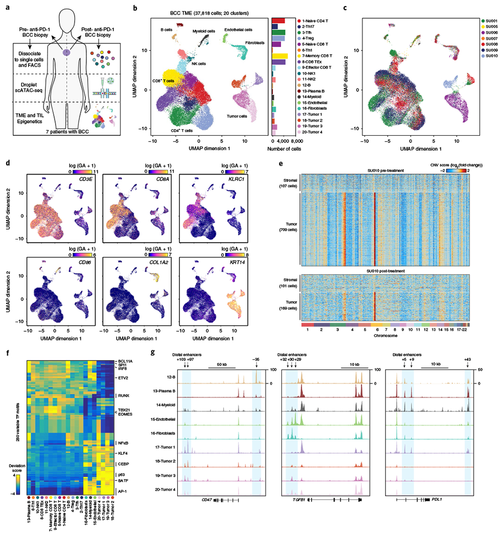
a, Schematic of analysis of BCC samples. b, UMAP projection of 37,818 scATAC-seq profiles of BCC TME cell types. Dots represent individual cells, and colors indicate cluster identity (labeled on the right). Bar plot indicates the number of cells in each cluster of cells. T cell clusters showed high CD3E, CD8A and CD4 gene scores; NK cell clusters: high KLRC1 and NCR1 gene scores; B cells and plasma cells: high CD19 and SDC1 gene scores, respectively; myeloid cells: high CD86, CSF1R and FLT3 gene scores; stromal endothelial cells and fibroblasts: high CD31 and COL1A2 gene scores, respectively; and tumor cell clusters: high KRT14 gene score. c, UMAP projection colored by patient of origin, as indicated on the right. d, UMAP projection colored by log-normalized gene scores demonstrating the accessibility of cis-regulatory elements linked (using Cicero) to the indicated gene. e, Estimated copy-number variation (log2(fold change) to GC-matched background) from scATAC-seq data. Stromal cells include endothelial cells and fibroblasts. f, Heatmap representation of ATAC-seq chromVAR bias-corrected deviations in the 250 most variable TFs across all scATAC-seq clusters. Cluster identities are indicated at the bottom of the plot. g, Genome tracks of aggregate scATAC-seq data, clustered as indicated in b. Arrows indicate the position and distance (in kb) of distal enhancers in each gene locus.
Classification of scATAC-seq clusters using cis-elements and gene scores revealed a diverse ecosystem of cell types in the BCC TME, including nine T cell clusters, two NK cell clusters, B cells and plasma cells, myeloid cells that comprised cDCs and macrophages, stromal endothelial cells and fibroblasts, and four tumor cell clusters (Fig. 4b–d and Supplementary Fig. 6e). Notably, stromal and immune cells from different patients largely clustered together, demonstrating that these clusters did not represent patient-specific cell states or batch effects. In contrast, tumor cell clusters were largely patient-specific, consistent with earlier single-cell RNA sequencing studies in melanoma and head and neck cancer39,40 (Fig. 4c and Supplementary Fig. 6f). To identify potential genome alterations in tumor cells, we estimated copy number variation (CNV) from scATAC-seq data (Fig. 4e and see Methods). This analysis revealed CNVs in tumor clusters 17–20, compared with other stromal cell populations. For example, tumor cells in patient SU010 showed ATAC-seq signal consistent with amplifications of regions of chromosomes 3 and 6, which were present in both pre- and post-therapy samples (Fig. 4e). Finally, we analyzed TF activity and found distinct patterns of activity in immune cells, compared with stromal or tumor cells (Fig. 4f and Supplementary Fig. 7a,b). In particular, tumor cells showed high accessibility of GLI1 motifs, consistent with the critical role of the Hedgehog pathway in BCC (Supplementary Fig. 7b)41.
Chromatin landscape of intratumoral TEx after PD-1 blockade.
Since T cells can be activated by targeting inhibitory receptors on T cells or inhibitory receptor ligands on stromal cells, we examined both cell populations. First, we analyzed cis-elements near genes encoding the known inhibitory ligands, CD47, TGFβ and PD-L1 (ref. 42–44), and identified distinct patterns of accessibility across stromal and tumor clusters (Fig. 4g). We identified three cis-elements in the CD47 locus, consistent with previously identified functional enhancers controlling CD47 expression (Fig. 4g)45. The tumor necrosis factor- and NFκB-responsive +97 kb and +103 kb enhancers were only accessible in tumor cells, supporting previous reports that tumor CD47 expression is responsive to inflammatory signals and contributes to escape from immune surveillance45. Similarly, we identified three cis-elements in the TGFB1 locus that were accessible in stromal cells, consistent with the expression pattern of this gene in primary tumors (Fig. 4g)43. We also identified three known cis-elements in the PDL1 locus46, which demonstrated shared accessibility in tumor cells, stromal cells, and myeloid and B cells, supporting the broad expression pattern of this ligand and common cis-regulatory elements in each cell type (Fig. 4g).
We next re-clustered 28,274 T cells and identified 19 subclusters, revealing a rich diversity of T cell phenotypes in the TME (Fig. 5a). CD8+ T cell states included naïve T cells, effector T cells, memory T cells and TEx (Fig. 5b and Supplementary Fig. 8a,b). We also identified an intermediate TEx cluster (cluster 16) that exhibited gene scores of both TEx and memory T cells (Fig. 5b). CD4+ T cell states included naïve T cells, Tregs, T helper 1 (Th1) cells, T helper 17 (Th17) cells and Tfh cells (Fig. 5b and Supplementary Fig. 8a–c). We focused on CD8+ TEx cells since this population is enriched for clonally expanded tumor-specific T cells39,47,48, and the irreversibility of the TEx epigenetic state may limit re-invigoration of T cells after PD-1 blockade49. Indeed, a comparison of pre- and post-PD-1 blockade profiles showed that TEx cells were highly expanded after therapy; more than 90% of TEx cells were derived from post-therapy biopsies, whereas memory and effector CD8+ clusters were equally derived from both time points (Fig. 5c). Notably, we also observed an expansion of Tfh cells post-therapy, suggesting that PD-1 blockade impacts both CD4+ and CD8+ cell states in the TME (Fig. 5c). Across all T cell states, we identified 35,147 cis-elements that exhibited cell type-specific accessibility (mean, 3,361 peaks per cluster; FDR < 0.01; Supplementary Fig. 8d). In TEx cells, we identified 4,598 such elements, demonstrating that human T cell exhaustion is accompanied by global remodeling of the chromatin accessibility landscape, consistent with previous studies in mice49–52. Analysis of individual TEx-specific enhancers identified regulatory elements in inhibitory receptor loci (Fig. 5d). For example, the PDCD1 locus (encoding PD-1) contained an intragenic cis-element (+5 kb) with specific accessibility in TEx cells, suggesting that the persistent expression of PD-1 in exhausted T cells is controlled by a single state-specific enhancer, and that the regulation of persistent PD-1 expression may be different in humans and mice50. CTLA4 and HAVCR2 loci showed TEx-specific activity of several distal cis-elements, compared with other CD8+ T cell states (Fig. 5d).
Fig. 5 |. Epigenomic regulators of T cell exhaustion after PD-1 blockade.
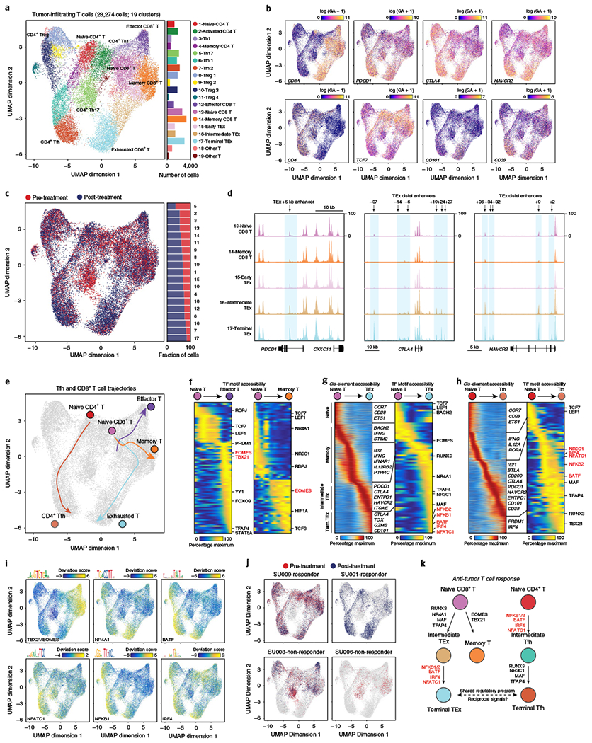
a, Subclustering UMAP projection of 28,274 tumor-infiltrating T cells (clusters 1–9 from TME UMAP). scATAC-seq profiles are colored by cluster identity, as labeled on the right. For CD8+ T cells, naïve T cells showed high CCR7 and TCF7 gene scores; effector T cells: high EOMES and IFNG gene scores; memory T cells: high EOMES gene score, but low effector gene scores; and exhausted T cells: high gene scores for inhibitory receptors PDCD1, CTLA4 and HAVCR2, and T cell dysfunction genes, CD101 and CD38. For CD4+ T cells, Tregs showed high FOXP3 and CTLA4 gene scores; Th1 cells: high IFNG and TBX21 gene scores; Th17 cells: high IL17A and CTSH gene scores; and Tfh cells: high CXCR5, IL21 and BTLA gene scores. Bar plot indicates the number of cells in each cluster of cells. b, UMAP projection colored by log-normalized gene scores demonstrating the accessibility of cis-regulatory elements linked (using Cicero) to the indicated gene. c, UMAP projection of tumor-infiltrating T cells colored by pre- and post-PD-1 blockade samples. d, Genome tracks of aggregate scATAC-seq data, clustered as indicated in a. Arrows indicate the position and distance (in kb) of intragenic or distal enhancers in each gene locus. e, Lineage trajectories of Tfh and CD8+ T cell states. Lines represent double-spline fitted trajectories across pseudotime. f, Pseudotime heatmap ordering of chromVAR TF motif bias-corrected deviations in effector and memory CD8+ T lineage trajectory. TF motifs are filtered for genes that are highly active (defined as the average percentile between total TF activity and variability > 0.75) that also demonstrate similarly dynamic gene scores across differentiation (R > 0.35 and FDR < 0.001 across 1,000 incremental groups). Heatmap of TF gene scores is shown on the right. g, Pseudotime heatmap ordering of cis-regulatory elements (left) and chromVAR TF motif bias-corrected deviations (right) in the CD8+ TEx lineage trajectory. h, Pseudotime heatmap ordering of cis-regulatory elements (left) and chromVAR TF motif bias-corrected deviations (right) in the CD4+ Tfh lineage trajectory. i, UMAP projection of scATAC-seq profiles colored by chromVAR TF motif bias-corrected deviations for the indicated factors. j, UMAP projection of tumor-infiltrating T cells colored by pre- and post-PD-1 in representative individual responder and nonresponder patients. k, Schematic of regulatory modules controlling TEx and Tfh differentiation.
We compared TEx differentiation trajectories with effector or memory CD8+ T cell trajectories (Fig. 5e). The differentiation of naïve CD8+ T cells to either effector or memory cells identified the critical roles of EOMES and TBX21 (T-bet) motifs in each pathway53–55 (Fig. 5f). Effector cell pseudotime also demonstrated the accessibility of other known regulator sites, including TFAP4 and YY1 (ref. 56,57). Similarly, memory cell pseudotime showed accessibility at HIF1A and E protein sites58. In contrast, TEx cells showed a distinct regulatory program, which progressed through two stages (Fig. 5g). The first stage (intermediate TEx) showed accessibility of cis-elements near inhibitory receptors, as well as elements near genes associated with tissue residency, such as ITGAE (CD103)59. Accordingly, this stage was accompanied by accessibility of NR3C1 and NR4A1 motifs, factors immediately downstream of T cell receptor (TCR) signaling that also induce exhaustion60,61, and the RUNX3 motif, a factor that programs tissue residency of CD8+ T cells (Fig. 5g)62. The second stage (terminal TEx) showed accessibility of cis-elements near genes associated with terminal T cell dysfunction, such as CD101 and TOX49,52,63–65, as well as of additional elements in stage 1 gene loci, such as CTLA4 (Fig. 5g). Importantly, this stage was accompanied by accessibility of a core set of TF motifs, which included NFKB1 and NFKB2, BATF, IRF4 and NFATC1, factors that are downstream of TCR signaling and have been demonstrated to play crucial roles in T cell exhaustion in mice66–68.
Finally, we examined the epigenetic relationship between TEx and Tfh cells. Tfh cells have previously been observed in tumors and are a prognostic indicator of response to checkpoint blockade69–71. The differentiation trajectory from CD4+ naïve T cells to Tfh cells showed accessibility of cis-elements neighboring Tfh-specific genes, such as IL21 and BTLA, but also of elements near genes typically associated with TEx cells, such as inhibitory receptors, consistent with the known, but unexplained, expression of these genes in human Tfh cells (Fig. 5h and Supplementary Fig. 8c–e)72. Strikingly, differentiation was accompanied by the accessibility of Tfh regulators, but also of the same core set of TF motifs associated with TEx differentiation, including NFKB2, BATF, IRF4 and NFATC1, suggesting a common program driving the development of TEx and Tfh cells downstream of PD-1 blockade (Fig. 5h,i and Supplementary Fig. 8f). Indeed, the +5 kb PDCD1 enhancer also showed high accessibility in Tfh cells and contained TF binding sites for the core TEx factors, IRF4 and BATF (Supplementary Fig. 8e). Finally, the abundance of TEx and Tfh cells was similar post-therapy, and, in our small cohort, the expansion of these cell types was greater in responder patients compared with nonresponder patients (Fig. 5j and Supplementary Fig. 9a, b). Altogether, these results map the epigenetic landscape of intratumoral TEx cells in humans and suggest that chronic TCR signals drive a shared regulatory program in TEx and Tfh cells after PD-1 blockade (Fig. 5k).
Discussion
The adoption of single-cell chromatin accessibility profiling has been hindered by trade-offs between data quality, throughput and cost. Here, we performed a droplet-based method for highly multiplexed single-cell chromatin accessibility profiling. scATAC-seq libraries generated using this method are high-quality, have a lower multiplet rate compared with previous methods, do not require cell sorting or noncommercial reagents and cost ~$0.4 per cell. The massive scale of cell type and cell state information generated by this method affords three key advantages: (1) comprehensive deconvolution of all cells in a tissue, including rare cells; (2) analysis of active regulatory DNA at the level of individual genes and cis-elements in single cells; and (3) unbiased reconstruction of developmental trajectories, without the use of predefined markers.
We used a data-driven approach to iteratively group single cells in the immune system together based on their accessible genomes, to reconstruct cell type-specific cis- and trans-regulatory maps and to highlight disease-associated enhancers that are active in specific cell types. Moreover, the density of single-cell clusters enabled computational inference of developmental trajectories, for example recapitulating decades of research on B cell and DC development. Importantly, scATAC-seq of tumor-infiltrating lymphocytes from patient biopsies identified regulatory programs controlling T cell exhaustion and a shared program with Tfh cells. Previous studies have demonstrated that chronic antigen stimulation drives the development of both TEx and Tfh cells73–75. Therefore, we speculate that this shared program may reflect an evolutionarily conserved pathway to synchronize CD4+ and CD8+ T cell responses to chronic pathogen infection, such that CD4+ Tfh cells support antibody formation as well as long-term activation of CD8+ T cells, perhaps through IL-21 (ref. 76–78). In summary, we describe the performance of a method for generating large-scale single-cell chromatin accessibility profiles on a widely distributed single-cell platform, enabling unbiased discovery of cell types and regulatory DNA elements in complex tissues.
Online content
Any methods, additional references, Nature Research reporting summaries, source data, statements of code and data availability and associated accession codes are available at https://doi.org/10.1038/s41587-019-0206-z.
Methods
Human subjects.
This study was approved by the Stanford University Administrative Panels on Human Subjects in Medical Research. Written informed consent was obtained from all participants, and all relevant ethical regulations regarding human research participants were followed.
Cell lines and PBMC/bone marrow samples.
Human (GM12878) and Mouse A20 (ATCC TIB-208) B lymphocytes were acquired and cultured according to guidelines from Coriell and the American Type Culture Collection, respectively. Fresh PBMCs, GM12878 and A20 cells were frozen according to the instructions outlined here: https://assets.ctfassets.net/an68im79xiti/2ptJYphPcPGfSPisq0cVuu/c8a83f93383c2fd1ce7cc49abc837992/CG000169_DemonstratedProtocol_NucleiIsolation_ATAC_Sequencing_Rev_B.pdf. Briefly, PBMCs were cryopreserved in IMDM + 40% FBS + 15% dimethylsulfoxide. GM12878 and A20 cells were cryopreserved in RPMI + 15% FBS + 5% dimethylsulfoxide. For monocyte and T cell mixing experiments, nuclei were first extracted and transposed, then mixed at indicated ratios. To avoid pipetting errors, a large number of nuclei were mixed after nuclei extraction and transposition, and a smaller number of nuclei were loaded onto the microfluidics chip for scATAC library generation. We also conducted a similar mixing experiment using naïve and memory T cells (Supplementary Table 2), which performed similarly and is included in the Data availability section.
Healthy volunteer PBMC and bone marrow samples were obtained from AllCells or the Stanford Blood Center. Mononuclear cells from each sample were isolated by Ficoll separation and cryopreserved in IMDM + 40% FBS + 15% dimethylsulfoxide. Samples were then thawed at 37 °C for 5 min and resuspended in media before cell enrichment using magnetic-activated cell sorting (MACS) or FACS (Supplementary Table 4). All MACS-enriched populations were obtained from AllCells and isolated per manufacturer recommendations (as outlined in Supplementary Table 4). FACS-isolated populations were obtained from AllCells or the Stanford Blood Center and sorted as follows. CD4+ T cells were sorted as naïve T cells (CD4+CD25−CD45RA+) or memory T cells (CD4+CD25−CD45RA−) using the following antibodies: anti-CD45RA-PERCPCy5.5 (clone HI100, cat. no. 304107, lot no. B213966, BioLegend), anti-CD4-APC-Cy7 (clone OKT4, cat. no. 317417, lot no. B207751, BioLegend) and anti-CD25-FITC (clone BC96, cat no. 302603, lot no. B168869, BioLegend). DCs and basophils were sorted as CD3−CD19−CD11c+HLA-DR+ (DCs) and CD3−CD19−CD123+ (basophils) using the following antibodies: anti-CD11C-PECy7 (clone B-ly6, cat. no. 561356, lot no. 4125556, BD Biosciences), anti-HLA-DR-APC-Cy7 (clone G46-6, cat. no. 335796, BD Biosciences), anti-CD123-BV421 (clone 6H6, cat. no. 306018, lot no. B156518, BioLegend), anti-CD3-FITC (clone OKT3, cat. no. 11-0037-41, lot no. 2007722, Invitrogen; dump gate) and anti-CD19-AlexaFluor 488 (clone HIB19, cat. no. 302219, lot no. B238185, BioLegend; dump gate). All antibodies were validated by the manufacturer in human peripheral blood samples, used at a 1:200 dilution, and compared with isotype and no staining control samples.
BCC sample collection and cell sorting.
All patients recruited for this study had locally advanced or metastatic BCC and were poor candidates for surgical resection. To minimize non-therapy-related immune cell variation, we excluded patients with previous exposures to checkpoint blockade, or to systemic immune suppressants within 4 weeks of biopsy. Fresh BCC biopsies were collected and digested in 5 ml DMEM/F12 + 250 μg ml−1 Liberase TL and 200 U ml−1 DNAse I with the gentleMACS Octo system at 37 °C for 3 h at 20 r.p.m. After tissue pieces were fully digested, 50 μl 500 mM EDTA was added and samples were collected by centrifugation at 300g for 5 min. Single-cell suspensions were filtered through 70 μm mesh and pelleted by centrifugation at 300g at 4 °C for 10 min. Finally, cells were resuspended in 1 ml RPMI and cryopreserved in FBS supplemented with 10% dimethylsulfoxide.
Cells were gently thawed at 37 °C for 5 min and resuspended in RPMI + 15% FBS before FACS. Cells were stained with anti-CD45 V500 (clone HI30, cat. no. 560779, lot no. 7172744, BD Biosciences), anti-CD3 FITC (clone OKT3, cat. no. 11–0037-41, lot no. 2007722, Invitrogen), anti-CD8 Pacific Blue (clone 3B5, cat. no. MHCD0828, lot no. 1964935, Invitrogen), anti-PD-1 APC/Cy7 (clone EH12.2H7, cat. no. 329921, lot no. B245235, BioLegend) and anti-HLA-DR eVolve 605 (clone LN3, cat. no. 83–9956-41, lot no. 1949784, Affymetrix-eBioscience). All antibodies were used at a 1:200 dilution, with the exception of anti-CD45 and anti-HLA-DR antibodies, which were used at a 1:100 dilution. Propidium iodide (cat. no. P3566, Invitrogen) was used for live/dead staining at a final concentration of 2.5 μg ml−1. Propidium iodide-negative live cells were sorted as T cells (CD45+CD3+), non-T immune cells (CD45+CD3−) or tumor/stromal cells (CD45−CD3−) and further processed using scATAC-seq.
scATAC-seq using the 10x Chromium platform.
All protocols to generate scATAC-seq data on the 10x Chromium platform, including sample preparation, library preparation and instrument and sequencing settings, are described below and are also available here: https://support.10xgenomics.com/single-cell-atac.
Nuclei isolation.
Isolation, washing and counting of nuclei suspensions were performed according to the Demonstrated Protocol: Nuclei Isolation for Single Cell ATAC Sequencing (10x Genomics). Briefly, 100,000 to 1,000,000 cells were added to a 2-ml microcentrifuge tube and centrifuged (300g· for 5 min at 4 °C). The supernatant was removed without disrupting the cell pellet, and 100 μl chilled Lysis Buffer (10 mM Tris-HCl (pH 7.4), 10 mM NaCl, 3 mM MgCl2, 0.1% Tween-20, 0.1% Nonidet P40 Substitute, 0.01% digitonin and 1% BSA) was added and pipette-mixed 10 times.
The microcentrifuge tube was then incubated on ice, with the length of time optimized for each cell type: GM12878 and A20 cell lines were incubated for 5 min, peripheral blood and bone marrow cells were incubated for 3 min and BCC cells were incubated for 3 min. Following lysis, 1 ml chilled Wash Buffer (10 mM Tris-HCl (pH 7.4), 10 mM NaCl, 3 mM MgĈ, 0.1% Tween-20 and 1% BSA) was added and the resulting solution was pipette-mixed 5 times. Nuclei were centrifuged (500g for 5 min at 4 °C) and the supernatant removed without disrupting the nuclei pellet. Nuclei were resuspended in chilled Diluted Nuclei Buffer (10x Genomics; 2000153) at approximately 5,000–7,000 nuclei per μl based on the starting number of cells. The resulting nuclei concentration was then determined using a Countess II FL Automated Cell Counter. Nuclei were then immediately used to generate scATAC-seq libraries as described in the methods and table below. For low-cell-number BCC samples (less than 20,000 cells), 2 modifications were made to the nuclei isolation protocol. First, 50 μl chilled Lysis Buffer was used instead of 100 μl chilled Lysis Buffer. Second, isolated nuclei were resuspended in 7 μl chilled Diluted Nuclei Buffer; 2 μl was used for cell counting, and 5 μl was used in the downstream library construction protocol.
Library construction.
scATAC-seq libraries were prepared according to the Chromium Single Cell ATAC Reagent Kits User Guide (10x Genomics; CG000168 Rev B). Briefly, after counting, nuclei concentrations were adjusted to the desired capture number, based on the number of available nuclei and the desired multiplet rate (described in the table below). A slightly higher number of nuclei were used to account for losses in subsequent steps. To minimize potential multiplets, we typically aimed to capture <6,000 nuclei per channel. Next, 5 μl of the resulting resuspended nuclei were combined with ATAC Buffer (10x Genomics; 2000122) and ATAC Enzyme (Tn5 transposase, 10x Genomics; 2000123/2000138) to form a transposition mix, which was then incubated for 60 min at 37 °C. The ATAC Buffer composition was derived from the Omni-ATAC buffer and designed based on quality control experiments in bulk cells, as previously described5. Mild detergent conditions were chosen to keep nuclei intact during tagmentation, as previously described5,8. A master mix composed of Barcoding Reagent (10x Genomics; 2000124), Reducing Agent B (10x Genomics; 2000087) and Barcoding Enzyme (10x Genomics; 2000125/2000139) was then added to the same tube as transposed nuclei. The resulting solution was loaded onto a Chromium Chip E (10x Genomics; 2000121) in a Chip Holder (10x Genomics; 330019). Vortexed Chromium Single Cell ATAC Gel Beads (10x Genomics; 2000132) and Partitioning Oil (10x Genomics; 220088) were also loaded onto the same Chromium Chip E before attaching a 10x Gasket (10x Genomics; 370017/3000072) and placing into a Chromium Single Cell Controller instrument (10x Genomics).
Approximately 100,000 GEMs are formed in each channel (8 channels per microfluidic chip), and approximately 80% of GEMs contain a single gel bead. Gel beads oligos were newly designed to consist of a 29-bp sequencing adapter, a 16 bp barcode selected from ~750,000 designed sequences (to index droplets) and the first 14 bp of read 1N (primers of the linear amplification reaction). Oligonucleotide sequences are provided below and in Supplementary Table 1 and are not chemically modified. Resulting single-cell GEMs were collected at the completion of the run (~7 min) and linear amplification was performed in a C1000 Touch Thermal cycler with 96-Deep Well Reaction Module (Bio-Rad; 1851197): 72 °C for 5 min, 98 °C for 30 s, cycled 12×: 98 °C for 10 s, 59 °C for 30 s and 72 °C for 1 min. Emulsions were coalesced using the Recovery Agent (10x Genomics; 220016), then subjected to Dynabeads (2000048) and SPRIselect reagent (Beckman Coulter; B23318) bead clean-ups. Indexed sequencing libraries were constructed by combining the barcoded linear amplification product with a sample index PCR mix comprising SI-PCR Primer B (10x Genomics; 2000128), Amp Mix (10x Genomics; 2000047/2000103) and Chromium i7 Sample Index Plate N, Set A (10x Genomics; 3000262). Amplification was performed in a C1000 Touch Thermal cycler with 96-Deep Well Reaction Module: 98 °C for 45 s, cycled variable amounts depending on cell load: 98 °C for 20 s, 67 °C for 30 s, 72 °C for 20 s, with a final extension of 72 °C for 1 min. The sequencing libraries were subjected to a final bead clean-up SPRIselect reagent and quantified by quantitative PCR (KAPA Biosystems Library Quantification Kit for Illumina platforms; KK4824). Sequencing libraries were loaded on an Illumina sequencer with 2 × 50 paired-end kits using the following read length: 50 bp read 1N, 8 bp i7 index, 16 bp i5 index and 50 bp read 2N. In the sequencing reaction, reads 1N and 2N contain the DNA insert, while the index reads, i5 and i7, capture the cell barcodes and sample indices, respectively.
scATAC-seq nuclei capture and sequencing specifications
| Nuclei capture desired | Resuspension concentration before ATAC reaction (nuclei per μl) | Volume used in ATAC reaction (μl) |
|---|---|---|
| 500 | 153 | 5 |
| 1,000 | 306 | 5 |
| 2,000 | 612 | 5 |
| 3,000 | 918 | 5 |
| 4,000 | 1,224 | 5 |
| 5,000 | 1,530 | 5 |
| 6,000 | 1,836 | 5 |
| 7,000 | 2,142 | 5 |
| 8,000 | 2,448 | 5 |
| 9,000 | 2,754 | 5 |
| 10,000 | 3,060 | 5 |
| Instrument | Loading concentration (pM) | PhiX (%) |
|---|---|---|
| NextSeq 500 | 1.7 | 1 |
| HiSeq 2500 (RR) | 11 | 1 |
| HiSeq 4000 | 180 | 1 |
| NovaSeq | 250 | 1 |
| Name | Sequence (5′–3′) |
|---|---|
| Read 1N | TCGTCGGCAGCGTCAGATGTGTATAAGAGACAG |
| Read 2N | GTCTCGTGGGCTCGGAGATGTGTATAAGAGACAG |
| Gel Bead Oligo Primer (PN-2000132) | AATGATACGGCGACCACCGAGATCTACAC-NNNNNNNNNNNNNNNN-TCGTCGGCAGCGTC |
| SI-PCR Primer B (PN-2000128) | AATGATACGGCGACCACCGAGA |
| i7 Sample Index Plate N, Set A (PN-3000262) | CAAGCAGAAGACGGCATACGAGAT-NNNNNNNN-GTCTCGTGGGCTCGG |
Availability of data processing and analysis software.
All data processing steps and methods used in the manuscript are described in detail below. We also have designed and made the following tools freely available:
Cell Ranger ATAC: This software performs initial data processing of scATAC-seq reads (including de-multiplexing, genome alignment and read deduplication), as described below and used in this manuscript. This software will also perform additional downstream analysis, including the identification of open chromatin regions, motif annotations and differential accessibility analysis, similar to what was performed in this manuscript and described at https://support.10xgenomics.com/single-cell-atac/software/pipelines/latest/what-is-cell-ranger-atac.
Loupe Cell Browser: This is an interactive visualization software that shows ATAC-seq peak profiles for scATAC-seq cell clusters, similar to the analysis done in this manuscript and described at https://support.10xgenomics.com/single-cell-atac/software/visualization/latest/what-is-loupe-cell-browser.
Data processing using Cell Ranger ATAC software.
The Cell Ranger Software (v.1.0; https://support.10xgenomics.com/single-cell-atac/software/pipelines/latest/algorithms/overview) was used for alignment, deduplication and identification of transposase cut sites. First, the 16-bp barcode sequence was processed to fix the occasional sequencing error in barcodes. Barcode sequences were obtained from the i5 index reads. An observed barcode not present in the whitelist of barcodes can be corrected to a whitelist barcode if it is within 2 Hamming distance away and has >90% probability of being the real barcode (based on the abundance of the barcode and quality value of incorrect bases). Then, the cutadapt tool was used to identify and trim any adapter sequence in each read. Third, the trimmed read pairs were aligned to a reference using BWA-MEM (Burrows-Wheeler Aligner Maximal Exact Matches algorithm) with default parameters. Reads less than 25 bp were not aligned and flagged as unmapped. Fragments were identified as read pairs with mapping quality (MAPQ) > 30, nonmitochondrial reads and not chimerically mapped. The start and end of the fragments were adjusted (+4 for +strand and −5 for –strand) to account for the 9-bp region that the transposase enzyme occupies during the transposition. Lastly, fragments with identical start and end positions were counted once. The most common barcode sequence was assigned to the fragments, with ties broken by picking the barcode sequence with the highest read counts. One of the read pairs with that barcode sequence was labeled as the ‘original’ and the other read pairs in the group were marked as duplicates of the fragment in the BAM file.
scATAC-seq data analysis.
Filtering cells by TSS enrichment and unique fragments.
Enrichment of ATAC-seq accessibility at TSSs was used to quantify data quality without the need for a defined peak set. Calculating enrichment at TSSs was performed as previously described46, and TSS positions were acquired from the Bioconductor package from ‘TxDb.Hsapiens.UCSC.hg19.knownGene. Briefly, Tn5-corrected insertions were aggregated ±2,000 bp relative to each unique TSS genome-wide (TSS strand-corrected). Then, this profile was normalized to the mean accessibility ±1,900–2,000 bp from the TSS and smoothed every 51 bp in R. The calculated TSS enrichment represents the maximum of the smoothed profile at the TSS. We then filtered all scATAC-seq profiles to keep those that had at least 1000 unique fragments and a TSS enrichment of 8. To minimize the contribution of potential doublets to our analysis, we removed scATAC-seq profiles that had more than 45,000 unique nuclear fragments.
Generating a counts matrix.
To make a cell by feature counts matrix, we first read each fragment into R using readr. Next, we converted fragment GenomicRanges into Tn5 insertion GenomicRanges by concatenating GenomicRanges for each ‘start’ and ‘end’ of the fragments (1 bp width). Next, we used ‘findOverlaps’ to find all overlaps with the feature by insertions. Then we added a column with the unique identity (ID) (integer) cell barcode to the overlaps object and fed this into a sparseMatrix in R. To calculate the fraction of Tn5 insertions in peaks, we used the colSums of the sparseMatrix and divided it by the number of insertions for each cell ID barcode using ‘table’ in R. The counts matrix was then log-normalized using edgeR’s ‘cpm(matrix, log = TRUE, prior.count = 3)’ in R. The prior count is used to lower the contribution of variance from elements with lower count values. This normalization assumes that differences in total chromatin accessibility across cell types are minor.
Generating union peak sets with LSI.
We created a union peak set by adapting a previous workflow12 as follows. Before calling peaks, we constructed 2.5-kb windows that were tiled across the genome by using ‘tile(hg19chromSizes, width = 2500)’ in R. Next, a cell-by-window sparse matrix was computed by counting the Tn5 insertion overlaps for each cell using ‘findOverlaps’ in R, as described above. This matrix was then binarized and pruned to the top 20,000 most accessible sites across all cells. We then reduced the dimensionality as previously described by computing the term frequency-inverse document frequency (TF-IDF) transformation9. Briefly, we divided each index by the colSums of the matrix to compute the cell ‘term frequency. Next, we multiplied these values by log(1 + ncol(matrix)/rowSums(matrix)), which represents the ‘inverse document frequency’. This normalization resulted in a TF-IDF matrix that was used as the input to irlba’s singular value decomposition (SVD) implementation in R. We then retained only the 2nd to 25th dimensions (first dimension was associated with cell read depth12) and created a Seurat object and identified crude clusters using Seurat’s SNN graph clustering (v.2.3) with ‘FindClusters’ with a default resolution of 0.8. If the minimum cluster size was below 200 cells, the resolution was decreased until this criterion was reached, leading to a final resolution of 0.8 × N (where N represents the iterations until the minimum cluster size is 200 cells).
The rationale for the 200-cell cut-off was to generate an initial cell clustering to identify confident ATAC-seq peaks (using MACS2 (ref. 17)) on grouped cells. It is important to note that this cut-off is only used for peak calling, and not for identifying cell types, and therefore rare cell types can still be clustered and analyzed in the final round of clustering. The theoretical ideal cluster size for the purpose of peak calling is the least number of cells required to recapitulate a bulk profile. In other words, the cluster should be large enough to capture bulk peaks, but small enough to preserve rare cell type clusters and peaks. To determine this number, we performed the down-sampling analyses shown in Supplementary Figs. 1d and 3f, which identified ~200 cells as a threshold at which ~70–80% of bulk peaks could be recovered in cell lines and primary cells. In samples where cell types of interest are likely to be significantly less frequent than 200 cells, we suggest the following workflow. A preliminary analysis of final clusters could be performed to determine the presence and frequency of rare cell types. If the cell type of interest is indeed less frequent than 200 cells, the number of cells sampled could be increased, or rare cells could be enriched before scATAC-seq to obtain a more accurate representation of accessible sites in this population.
Peak calling for each cluster was performed independently to get high-quality, fixed-width, nonoverlapping peaks that represent the epigenetic diversity of all samples46. For each cluster, peak calling was performed on Tn5-corrected singlebase insertions (each end of the Tn5-corrected fragments) using the MACS2 callpeak command with parameters ‘–shift -75–extsize 150–nomodel–call-summits–nolambda–keep-dup all -q 0.05’. The peak summits were then extended by 250 bp on either side to a final width of 501 bp, filtered by the ENCODE hg19 blacklist (https://www.encodeproject.org/annotations/ENCSR636HFF/) and then filtered to remove peaks that extended beyond the ends of chromosomes.
Overlapping peaks called within a single sample were handled using an iterative removal procedure as previously described46. First, the most significant peak was kept and any peak that directly overlapped with that significant peak was removed. Then, this process was iterated to the next most significant peak and so on until all peaks were either kept or removed due to direct overlap with a more significant peak. This was performed on each cluster’s peak set, and the top 200000 extended summits (ranked by MACS2 score) were retained, generating a ‘cluster-specific peak set’ for each cluster. We then normalized the MACS2 peak scores (−log10(Q value)) for each sample and converted them to a ‘score quantile’ by converting each individual score to a quantile using ‘trunc(rank(v))/length(v)’ in R (where v represents the vector of MACS2 peaks scores). This normalization method allowed for direct comparisons of peaks across clusters, enabling the generation of a union peak set for each dataset.
We next compiled a union peak set containing the important peaks observed across all clusters. First, all cluster peak sets were combined into a cumulative peak set and trimmed for overlap using the same iterative procedure mentioned above. Again, this procedure kept the most significant (in this case, score quantile) peak and discarded any peak that overlapped directly with the most significant peak. Lastly, we removed any peaks that spanned a genomic region containing ‘N nucleotides and any peaks mapping to the Y chromosome.
Reads-in-peaks-normalized bigwigs and sequencing tracks.
To visualize ATAC-seq cluster data, we created ATAC-seq signal tracks that were normalized by the number of reads in peaks, as previously described46. Briefly, we created fragment files that contained all cells belonging to a specific cluster and then counted the number of Tn5 insertions in the corresponding peak set. The numbers of Tn5 insertions were computed in windows genome-wide using ‘slidingWindows(chromSizes,100,100)’. Next, we created a run-length encoding using ‘coverage’ in R and normalized the total reads to a scale factor that normalized the reads-in-peaks to 10 million reads within peaks. This object was then converted into a bigwig using rtracklayer ‘export.bw’ in R. For plotting tracks, the bigwigs were read into R using rtracklayer ‘import.bw(as = ”Rle”)’ and plotted within R or visualized with WashU Epigenome browser (public browser session links included below). All track figures in this study show groups of tracks with matched normalized y axis scales.
To visualize scATAC-seq data, we read the fragments into a GenomicRanges object in R. We then computed 100-bp sliding windows across each visualized region with ‘slidingWindows(region,100,100)’. We computed a counts matrix for Tn5-corrected insertions as described above and then binarized this matrix. We then returned all nonzero indices from the matrix (cell X 100 bp intervals) and plotted them in ggplot2 in R with ‘geom_tile’
ATAC-seq-centric LSI clustering and visualization.
We clustered scATAC-seq data using an approach that did not require bulk data or previous knowledge. To achieve this, we adopted the strategy by Cusanovich et. al.9, to compute the TF-IDF transformation. Briefly, we divided each index by the colSums of the matrix to compute the cell ‘term frequency’. Next, we multiplied these values by log(1 + ncol(matrix)/rowSums(matrix)), which represents the ‘inverse document frequency’ This resulted in a TF-IDF matrix that was used as input to irlba’s SVD implementation in R. We then used the first 50 reduced dimensions as input into a Seurat object, and crude clusters were identified using Seurat’s (v2.3) SNN graph clustering ‘FindClusters’ with a default resolution of 0.8. We found that there was detectable batch effect that confounded further analyses. To attenuate this batch effect, we calculated the cluster sums from the binarized accessibility matrix and then log-normalized using edgeR’s ‘cpm(matrix, log = TRUE, prior.count = 3)’ in R. Next, we identified the top 25,000 varying peaks across all clusters using ‘rowVars’ in R. This was done on the cluster log-normalized matrix rather than the sparse binary matrix because: (1) it reduced biases due to cluster cell sizes, and (2) it attenuated the mean-variability relationship by converting to log space with a scaled prior count. The 25,000 variable peaks were then used to subset the sparse binarized accessibility matrix and recompute the TF-IDF transform. We used SVD on the TF-IDF matrix to generate a lower dimensional representation of the data by retaining the first 50 dimensions. We then used these reduced dimensions as input into a Seurat object and crude clusters were identified using Seurat’s (v.2.3) SNN graph clustering ‘FindClusters’ with a default resolution of 0.8. These same reduced dimensions were used as input to Seurat’s ‘RunUMAP’ with default parameters and plotted in ggplot2 using R.
For subclustering analyses (hematopoiesis: CD34+ bone marrow and DCs; tumor: T cells), we computed the cluster sums again and log-normalized using edgeR’s ‘cpm(matrix, log = TRUE, prior.count = 3)’ in R. We identified the top 10,000 and 5,000 varying peaks for CD34+ cells and T cells, respectively. These variable peaks were then used to subset the sparse binarized accessibility matrix and recompute the TF-IDF transform. We then used SVD on the TF-IDF matrix to generate a lower dimensional representation of the data by retaining the first 25 dimensions. We then used these reduced dimensions (1–25 and 2–25, respectively) as input into a Seurat object, and then crude clusters were identified using Seurat’s (v2.3) SNN graph clustering ‘FindClusters’ with a default resolution of 0.8. These same reduced dimensions were used as input to Seurat’s ‘RunUMAP’ and plotted in ggplot using R.
Inferring copy number amplification.
To infer DNA copy number amplifications from scATAC-seq data, we adapted an approach previously used for bulk ATAC-seq data46,79,80. This method estimates CNVs by determining read counts in large intervals across the genome and comparing read counts in each interval with the average read count in 100 GC-matched intervals. To overcome the sparsity of scATAC-seq data, we made two modifications. First, we increased the interval size to 10 Mb (rather than 2 Mb). Second, in each sample, we compared CNV signals in tumor cells with those in nontumor cells. CNVs present in both groups are unlikely to represent tumor-relevant CNVs. To do this, we first tiled the genome into 10-Mb windows using ‘slidingWindows’ of GenomicRanges for chromosome sizes in R with a step size of 2 Mb. These window positions were then filtered against regions with known artifactual mapping issues using the ENCODE hg19 blacklist with the ‘setdiff’ function in R. Then, a cell-by-window binarized matrix was constructed, as described above. Next, the insertions per bp was determined within each filtered 10-Mb window. The percentage GC nucleotide content was computed for each filtered 10-Mb window using the hg19 BSgenome in R. To estimate whether a region is amplified, we identified the 100 nearest neighbors based on GC content and computed the average log2(fold change). If this was above 1, we considered this region a candidate for amplification. This approach was previously validated in bulk ATAC-seq data46. However, we also validated its accuracy with matched whole exome sequencing data from an earlier study in two patient samples (SU006 and SU008 pretreatment)48. Indeed, CNVs identified using scATAC-seq were confirmed by whole exome sequencing.
TF footprinting.
We characterized relative TF occupancy through TF footprints, as previously described46. For each peak set, we used Catalog of Inferred Sequence Binding Preferences (CIS-BP) motifs (from chromVAR motifs human_pwms_v1) to calculate motif positions using motifmatchr ‘matchMotifs(positions = “out”)’ Next, we computed the Tn5 bias for each sample by constructing a hexamer bias table using ‘oligonucleotidefrequency’ function from Biostrings in R. Then, we calculated a hexamer table for each TF by counting the hexamers relative to each stranded motif position ±250 bp from the motif center. Using the sample’s hexamer frequency table, we could then compute the expected Tn5 insertions by multiplying the hexamer position frequency table by the observed/expected Tn5 hexamer frequency. For analysis of TF motifs present in the +5 kb enhancer of PDCD1, we searched for CIS-BP motifs with a LogOdds threshold greater than 10.
To assess the reproducibility of footprints, we subsampled fragments in each cluster 2 times at a sampling rate of 60% to have maximum variability. To calculate the insertions around these sites, we converted the Tn5-corrected insertions GenomicRanges (see above) into a coverage run-length encoding using ‘coverage’. For each individual motif, we iterated over the chromosomes, computing a ‘Views’ object using ‘Views(coverage, motif positions)’. This ‘Views’ object was converted to a matrix using ‘as.matrix’ and the colSums for ‘-stranded’ motifs were reversed and the colSums for not ‘-stranded’ motifs were summed. To better compare footprints across samples, we normalized these footprints by the mean values ±200–250 bp from the motif center. Next, we divided the footprints by the expected Tn5 bias to attempt to account for the inherent Tn5 bias. While this strategy is effective, it does not fully account for all of Tn5’s sequence bias. We then plotted the mean and standard deviation for each footprint pseudo-replicate.
ChromVAR.
In addition to TF footprinting, we measured global TF activity using chromVAR4. As input we used the raw insertion counts for all peaks and the CIS-BP motif (from chromVAR motifs ‘human_pwms_v1’) matches within these peaks from motifmatchr. We then computed the GC bias-corrected deviation scores using the chromVAR ‘deviationScores’ function. All plots used the ‘deviationScores’ in R and variability was computed by using ‘rowVars’ in R.
Computing gene activity scores using Cicero co-accessibility.
We calculated gene activity scores (gene scores) using the R package Cicero, as previously described19. Briefly, Cicero calculates peak-to-peak links based on their co-accessibility across groups of cells that are aggregated using a nearest-neighbor approach (k = 50). After peak-to-peak links are identified using cell groups, ATAC-seq counts within co-accessible sites (for example, linked to a specific gene) can be calculated and visualized in each single cell in the total dataset. We first used the sparse binary matrix and created cellDataSet, detectedGenes and estimatedSizeFactors. Next, we created a ‘cicero_cds’ with k = 50 and the ‘reduced_coordinates’ from the corresponding UMAP coordinates. This function returns aggregated accessibility across groupings of cells based on nearest-neighbor rules. We then used this aggregated accessibility matrix to identify all peak-to-peak linkages that were within 250 kb by resizing the peaks to 250 kb and then overlapping them with the peak summits/centers. We removed all duplicates and same peak-to-peak links. Next, we calculated the Pearson correlation for each peak-to-peak link and created a connections data.frame where the first column was peaki, the second column was peakj and the third column was co-accessibility (Pearson correlation). We then created a gene data.frame by retrieving genes from the TxDb ‘TxDb.Hsapiens. UCSC.hg19.knownGene’ in R. We altered the start of ‘MEF2C’ to 88014057, since this alternative TSS demonstrated stronger promoter accessibility. We then resized each gene to its TSS and created a window ±2.5 kb from the TSS and then annotated the ‘cicero_cds’ using ‘annotate_cds_by_site’. We then calculated gene scores for each scATAC-seq profile using ‘build_gene_activity_matrix’ with a co-accessibility cut-off of 0.35. Lastly, we normalized the gene scores using ‘normalize_gene_activities’ and the read depth of the cells. We adapted gene activity (GA) scores to be more interpretable by further log normalizing by computing ‘log2(GA*1000000 + 1), which we refer to in the text as ‘log2(GA + 1). This conversion is analogous to log counts per million (CPM) transformation and allowed gene scores to be used further in TF deduplication and cell annotations. The resulting matrix was used to visualize gene scores with single-cell resolution using UMAP.
Analysis of autoimmune variants using Cicero co-accessibility and chromVAR.
We sought to characterize cell type-specific enrichments in known disease-associated regulatory elements. To perform this analysis, we downloaded causal single nucleotide polymorphisms (SNPs) for 39 diseases from http://pubs.broadinstitute.org/pubs/finemapping/dataportal.php. We then converted SNPs into a GenomicRanges object and overlapped them with ATAC-seq peaks. To increase the power of this analysis, beyond direct overlaps, we used Cicero co-accessibility links to include peaks that were co-accessible with those containing SNPs. To do this analysis, for every peak with an SNP overlap, we calculated and included peaks that were co-accessible above 0.35. We then created an overlap matrix for every group of SNPs partitioned by disease. Finally, we used this as input to chromVAR’s ‘computeDeviations’ with the scATAC-seq raw insertion counts for all peaks. We used the ‘deviationScores’ from chromVAR and plotted the median score across each cluster in R.
HiChIP meta-virtual 4C (metav4C) analysis for Cicero co-accessibility links.
We further validated predicted Cicero co-accessibility links using previously published chromosome conformation data, as previously described46. Briefly, we used published H3K27ac HiChIP data from primary T cell subsets22 (naïve, Th17 and Treg) to support predicted Cicero co-accessibility links. First, we converted peak-to-gene links to 10-kb resolution by flooring each coordinate (gene start and peak center) to the nearest 10-kb window and deduplicated. To make distance-scaled metav4C plots, each chromosome was retrieved from the ‘.hic’ interactions file using juicer dump at 10-kb resolution and read into a ‘sparseMatrix’ in R (each coordinate in the matrix corresponding to a 10-kb interaction bin). Then, for each peak-to-gene link longer than 100 kb, the upstream or downstream window (depending on the peak’s location relative to the TSS) was identified and then interpolated linearly using the ‘approx’ function to get the value at each 0.1% position. The normalized reads at each 0.1% position for each peak-to-gene link were then summed and divided by the total number of peak-to-gene links. Normalization of H3K27ac HiChIP data was performed as previously described22. Replicate reproducibility was visualized with the mean profile shown as a line and the shading surrounding the mean representing the standard deviation between replicates. Lastly, we wanted to test the specificity of scATAC-seq T cell clusters in naïve, Th17 and Treg H3K27ac HiChIP data. We computed the cluster sums for each cluster from the binarized accessibility matrix for clusters 21 (naïve), 24 (memory) and 25 (Treg), log-normalized, and computed the row-wise Z-scores, where each row represents a unique ATAC-seq peak. We then took the top 25,000 peaks by Z-score for each cluster and overlapped these with Cicero links. We then plotted the metav4C for each of the three T cell subtypes with replicate reproducibility as described above. To further compare the overlap between co-accessibility links and H3K27ac HiChIP, we used Fit-Hi-C81 to create a union set of chromatin contacts from T cell HiChIP data at 10-kb resolution22. We binned co-accessibility links (identified in all immune cells) to 10-kb resolution and determined that ~12% of links were also present in H3K27ac HiChIP T cell chromatin contacts (compared with a permuted background of n = 10,000 links, with an average overlap of ~4%, P < 0.0001).
Overlap of Cicero co-accessibility links with GTEx eQTLs.
eQTLs from the Genotype-Tissue Expression project were used to support the scATAC-seq-defined Cicero co-accessibility links as previously described46. First, we identified all gene starts from gencode v.19 (https://gtexportal.org/home/datasets) and extended them ±2.5 kb, as we did when computing gene scores, and then overlapped all peaks with these regions using findOverlaps. We then labeled peaks that overlapped with the extended gene starts as promoter peaks and identified all ATAC-seq peak-to-promoter links. We chose to do this analysis with gencode v19 to match gene identities to those in the eQTL dataset. GTEx eQTL data (v.7) was downloaded from https://gtexportal.org/home/datasets and the *.signif_variant_gene_pairs.txt. gz files were used. All eQTLs located more than 250 kb away from the predicted gene pair were removed to maintain consistency with the 250-kb window used in predicting ATAC-seq peak-to-gene links. We were particularly interested in testing distant peak-to-gene predictions from Cicero, since genes nearest to a peak are easily predicted without co-accessibility calculations. To achieve this, the nearest gene for each eQTL was determined using ‘distanceToNearest’ with the eQTL regions to all gene starts in gencode v19 in R, and all eQTL-nearest gene links were removed. The remaining eQTLs impacted genes that were not simply the nearest neighboring gene and thus could be used to test the predictive power of the non-nearest-gene peak-to-gene link predictions from Cicero. All peak-to-gene links were then overlapped with these filtered eQTLs using ‘findOverlaps’ and then matched based on the predicted linked gene. To assess the significance of these overlaps, we created 250 random peak-to-gene link sets by taking all peaks from the hematopoiesis union peak set and randomly assigning these peaks to any gene within 250 kb of the peak summit. Then, we calculated the Z-score and enrichment of our determined peak-to-gene links compared with the randomized peak sets.
We then calculated the adjusted P value using the Benjamini-Hochberg correction. Overall, this provided a conservative overlap estimate of ~5% across eQTL sets with nearest gene removal (~2-fold enrichment compared with a permuted background of peak-to-gene links, P < 0.0001). Although eQTLs from several tissues were enriched in peak-to-gene links, possibly reflecting common usage of many enhancers across cell types, the greatest enrichment was observed in immune tissues (spleen, whole blood, lymphocytes), as expected.
Constructing ATAC-seq pseudo-bulk replicates of maximal variance.
We wanted to perform analyses that treated each cluster as a bulk ATAC-seq sample but required a method that could create replicates that convey close to the true population variance within a cluster and potential batch effects. To achieve this, for each cluster, we first checked whether the cluster contained 2 or more independent 10x experiments that each contributed at least 100 cells to the cluster. If true, then independent 10x experiment cells were summed from the binarized matrix (maximum of 500 cells randomly sampled) to create pseudo-bulk replicates. If this condition was not met for a cluster, but there was at least 1 10x experiment that had at least 100 cells and there were at least 100 cells left over, then we used the following procedure. First, 1 10x experiment was summed from the binarized matrix (maximum of 500 cells randomly sampled) to create a pseudo-bulk replicate. Second, for the remaining cells, we constructed a pseudo-bulk replicate by randomly sampling 100 cells, 250 times, and we used the sampling that pro duced the highest within-cluster total log-variance (cpm(mat, log = TRUE, prior.count = 3) then summed ‘rowVars’ with the 1 10x experimental replicate). If the cluster did not contain 1 10x experiment with at least 100 cells, then 2 replicates of 100 cells were randomly sampled 250 times, and we used the sampling that produced the highest within-cluster total variance (cpm(mat, log = TRUE, prior. count = 3) then summed ‘rowVars’ with both sampled replicates). Finally, if the cluster was smaller than 150 total cells, the number of cells sampled was two-thirds the total size of the cluster. This workflow was designed to construct pseudo-replicates from single-cell clusters that produced high variance to attempt to capture true biological variation. In general, this approach is still an underestimate of variation when fully simulating replicates, so it is important to be conservative when using these pseudo-replicates in further analyses.
Constructing gene score pseudo-bulk replicates of maximal variance.
To construct pseudo-bulks for gene scores, we followed a similar procedure as just described above using the log(GA + 1) matrix. If a cluster contained 2 or more independent 10x experiments that each contributed at least 100 cells, then cells from independent experiments were averaged from the log(GA + 1) matrix (maximum of 500 cells randomly sampled) to create pseudo-bulk replicates. If the cluster contained 1 10x experiment with at least 100 cells and an additional 100 cells, then the 1 10x run was averaged from the log(GA + 1) matrix (maximum of 500 cells randomly sampled) to create a pseudo-bulk replicate, and the remaining cells were used to create another pseudo-bulk replicate by randomly sampling 100 cells, 250 times, and we used the sampling that produced the highest within-cluster total log-variance (summed ‘rowVars’ with the 1 10x run replicate). If the cluster did not contain 1 10x experiment with at least 100 cells, then 2 replicates of 100 cells were randomly sampled 250 times, and we used the sampling that produced the highest within-cluster total variance (summed ‘rowVars’ with both sampled replicates). Lastly if the cluster was smaller than 150 total cells, the number of cells sampled was two-thirds the total size of the cluster.
Identification of cluster-specific peaks and gene scores through feature binarization.
Once we determined clusters from scATAC-seq data, we identified peaks that were uniquely present within each cluster or combination of clusters. We modified a previously described approach to binarize each feature and then identify unique features in a simplistic manner46. For ATAC-seq, we used bulk pseudo-replicates and log-normalized the matrix using ‘edgeR::cpm(mat,log = TRUE,prior. count = 3)’. For gene scores, we used bulk pseudo-replicates and normalized the matrix by first converting to gene scores and then converting back to log by computing ‘log2(edgeR::cpm(2^logMat-1) +1)’. We then computed the mean and standard deviation for each cluster using ‘rowMeans’ and ‘rowSds’, respectively, in R. Next, for each feature peak or gene, we ranked the clusters by their intra-cluster mean. Then, we iterated from the second lowest cluster, determining whether the mean of that cluster: (1) was greater than the maximum intra-cluster mean plus 0.5 times the intra-cluster standard deviation of the next-lowest cluster (1 s.d. for subcluster binarization), and (2) was greater than log2FC (fold change) to the maximum intra-cluster mean of 0.25. This process was continued and the last time this criterion was met was labeled as the ‘break point’, and all clusters above this intra-cluster mean were marked with a ‘1’ and below with a ‘0. If a peak did not have a break point, it was discarded. This binarization will capture peaks that are unique to multiple groups. Next, all classified peaks/genes that corresponded to more than a total of the floor of one-third of the clusters were used as input. Next, for each peak/gene, a two-sided t-test was computed comparing all ‘1’s’ and ‘0’s, and the P values were adjusted for multiple hypotheses through the Benjamini-Hochberg correction by ‘p.adjust(method = “fdr”)’. All peaks/genes that had an adjusted P value below 0.01 were kept. Lastly, we filtered out all binarization patterns that were classified less than 25 times. These were then plotted in R using the package ComplexHeatmap.
Pseudotime analysis.
To order cells in pseudotime, we sought to identify a trajectory and then align single cells across the trajectory. We chose to use UMAP for alignment if cells were part of a continuous substructure, since local distances are better preserved using this framework. We note that since input parameters can change the resulting UMAP, it is important to be cautious when constructing trajectories in this subspace. First, we described candidate trajectories by ordering clusters. Next, for each cluster, we calculated the mean coordinates in both dimensions and filtered cells that were in the top 5% Euclidean distance to the mean coordinates. We computed the UMAP distance for each cell from clusteri to the mean coordinates of clusteri+1 along the trajectory. We then computed a pseudotime vector by calculating the quantiles for each cell by their distance to the next cluster and added the current iteration. This allowed us to obtain a UMAP coordinate and a time component for each cell. Next, we fit a continuous trajectory to both UMAP coordinates using ‘smooth.spline’ with degrees of freedom (dof) = 250 and smoothing parameter (spar) = 1. Then, we aligned all cells to the trajectory by their Euclidean distance to the nearest point along the manifold. We computed and scaled this alignment to 100 and used this as pseudotime for further analyses.
To further support longer trajectories in pseudotime, we evaluated the significance of the trajectory by its cluster ordering. To evaluate trajectories, we took the latest cluster, ranked the top 10,000 accessible peaks and then computed the Euclidean distance to all other clusters (logCPM). We then continued in this reverse trajectory and computed the distance to all other clusters that did not include the previous clusters for directionality. To determine the significance of the ordering, we permuted the ordering of the trajectory 5,000 times and computed the average rank of the ordering for the permuted and input trajectory. This allowed for an empirical P value calculation that we could assign to each reduced dimension trajectory from the original accessibility matrix.
We then sought to create matrices that conveyed feature trends across pseudotime. To perform this analysis, we ordered the cells by their pseudotime and fit a smoothed line for each feature by using ‘geom_smooth’ with method ‘gam’ and formula ‘y ~ s(x, bs = “cs”)’ and n = 100. For peaks, we used the binarized sparse accessibility matrix. For gene scores, we used the log-normalized (log(GA + 1)) matrix. For TF motifs, we used the chromVAR deviation score matrix. We deduplicated chromVAR CIS-BP motifs by correlating the gene score of a TF to the inferred activity of the TF in chromVAR. We correlated TFs and their corresponding gene scores, and then, using cor.test in R, we calculated the associated P value and adjusted for multiple hypotheses through the Benjamini-Hochberg correction by ‘p.adjust(method = “fdr”)’. Next, we computed the quantile for each TF’s gene score average and variance. We then averaged these quantiles to equally weight the log-average gene score and log-variance. We then filtered the top 25% of TFs by this criterion, and then further by TF motif pairs that were correlated above 0.35 and FDR < 0.001. These were then used to identify TF motif pairs that were more likely to be involved in gene regulation across the identified pseudotime.
Barnyard mixing analysis.
We assessed the rate at which multiplets (more than one cell per droplet) occurred at different cell loadings in our data. To calculate this rate, we performed human (GM12878) and mouse (A20) mixing experiments at loadings of 500, 1,000, 5,000 and 10,000 cells. We aligned the data using 10x Cell Ranger v.1.0. We then removed low-quality cells as described above using both hg19 and mm10 genomes (TSS enrichment of 8 and 1,000 unique fragments). Next, we determined the effective multiplet rate by comparing the fragments aligning to each genome within scATAC-seq profiles. We labeled a scATAC-seq profile as a multiplet if less than 95% of the unique nuclear fragments aligned to either hg19 or mm10. Since multiplets could involve 2 or more nuclei of the same type (GM12878 or A20) and barnyard samples were prepared as 50:50 mixtures, we multiplied the effective multiplet rate by 2 to reach the estimated multiplet rate.
We then determined the effects of different numbers of cells and unique nuclear fragments on ATAC-seq peak recovery by down-sampling cells and unique fragments in silico. We did this analysis by merging all GM12878 and A20 fragments from the mixing experiments into one fragments file. Next, we down-sampled the fragments file first by the number of cells and then by the number of fragments to make the unique fragments per cell match the desired output. We then called peaks on each down-sampled file by creating a bed file of the Tn5 insertions (ends of the fragments) with MACS2 callpeak command with parameters ‘–shift -75–extsize 150–nomodel–call-summits–nolambda–keep-dup all -q 0.05’. The peak summits were then extended by 250 bp on either side to a final width of 501 bp, filtered by the ENCODE hg19 blacklist (https://www.encodeproject.org/annotations/ENCSR636HFF/) and then filtered to remove peaks that extended beyond the ends of chromosomes. We then took the top 100,000 nonoverlapping extended summits, as previously described46. We repeated this on the total fragments file to get a GM12878 and A20 peak set. Next, we computed the fraction of peaks recovered by using ‘countOverlaps’ and dividing by the extended summits of the total fragments file in R. Lastly, we counted the number of Tn5 insertions for each down-sampled fragments file within the GM12878 and A20 peak set, log-normalized the matrix with ‘edgeR::cpm(mat, log = TRUE, prior. count = 3)’ and computed the Pearson correlation. We then plotted the results in R using ‘ggplot’.
Analysis of fresh versus frozen PBMCs.
We compared the effect of sample preparation on scATAC-seq data quality. To do this, we performed scATAC-seq on PBMCs that were freshly isolated, frozen or frozen and sorted for live cells. We filtered the cells as described above (TSS enrichment 8 and 1,000 unique fragments) and then used our TF-IDF cluster peak-calling framework to generate a peak set for each experiment. We then used our TF-IDF cluster analysis as described above (top 25,000 variable peaks with SVD dimensions 1–50) and computed clusters for each experiment. We performed principal component analysis on the cluster sums identified and used all fresh peaks for the analysis. To compare at the single-cell level, we created a cell-by-counts matrix for each fresh, frozen and frozen sorted sample using fresh sample peaks. We then used our TF-IDF cluster analysis (top 10,000 variable peaks with SVD dimensions 1–25) and projected onto a UMAP using ‘RunUMAP’ form Seurat in R. We then computed the receiver operating characteristic and precision-versus-recall curves for frozen and frozen sorted samples against the fresh sample by using ‘overlapsAny’, ranking the peaks by MACS2 score, and using this as input into ‘pr.curve’ or ‘roc.curve’ from the package PRROC in R. The true positives in these curves were defined as peaks identified in fresh PBMCs. Finally, we conducted principal component analysis with ‘prcomp’ and computed correlations of clusters between experiments with the fresh sample ATAC-seq peaks.
Spike-in analysis.
We tested the sensitivity and performance of our analysis workflow by performing scATAC-seq on monocyte and T cell mixtures at various loadings. We filtered the cells as described above (TSS enrichment 8 and 1,000 unique fragments) and then used our TF-IDF cluster peak calling framework to generate a peak set for each experiment. We then used TF-IDF cluster analysis as described above (top 25,000 variable peaks with SVD dimensions 1–50) and computed clusters for each experiment. We used ‘RunUMAP’ with default parameters from Seurat (v2.3) to compute a UMAP for each spike-in experiment and computed gene scores as described above by using the full hematopoiesis peak set, accessibility matrix and co-accessible links, and added each sample individually for calculating the gene scores. We computed a monocyte score by taking the log(GA + 1) average for CD14, MAFB, HLA-DRB1, TREML4, CSF1R, CEBPA, TLR4, HLA-DRA and CD74. We computed a T cell score by taking the log(GA + 1) average for CD3E, CD2, CD5, CD7, IL7R, IL2, TCF7, CD3D and CD3G. For integrative analysis of all mixing experiments to test for batch effects, we merged all peaks identified in each individual experiment to create a union peak set. We then performed clustering as described above to visualize single-cell clusters on one UMAP.
Reporting Summary.
Further information on research design is available in the Nature Research Reporting Summary linked to this article.
Data availability
All single-cell sequencing data are available through the Gene Expression Omnibus under accession GSE129785. There are no restrictions on data availability or use. Species-mixing and PBMC datasets are available in pre- and post-processed formats here: https://support.10xgenomics.com/single-cell-atac/datasets. WashU browser sessions of aggregated scATAC-seq data (by cluster, as shown in each Figure) are available here: Fig. 2 single-cell clusters: http://epigenomegateway.wustl.edu/legacy/?genome=hg19&session=HcbHMSgBCc&statusId=28207718. Fig. 4 single-cell clusters: http://epigenomegateway.wustl.edu/legacy/?genome=hg19&session=tYJVrV7zzk&statusId=834543265. Fig. 5 single-cell clusters: http://epigenomegateway.wustl.edu/legacy/?genome=hg19&session=7UZG0iF90b&statusId=807471043. Whole exome sequencing data from patients SU006 and SU008 were previously described48 and obtained from the Sequence Read Archive under accession PRJNA533341.
Code availability
Custom code for main analyses used in this work has been deposited on GitHub: https://github.com/GreenleafLab/10x-scATAC-2019.
Supplementary Material
Acknowledgements
We thank members of the Chang and Greenleaf laboratories and 10x Genomics for helpful discussions. We thank the following people at 10x Genomics: A. Puleo for sorting cells, J. Chevillet for training, Z. Bent and M. Dodge for reagents development, R. Gerver and W. Wang for microfluidics and A. Gallegos, A. Gonzales, N. Keivanfar, S. Maheshwari, P. Marks, J. Mellen, R. Rico and K. Wu for computational and software support. We thank X. Ji, D. Wagh and J. Coller at the Stanford Functional Genomics Facility and C. Bruce at 10x Genomics for sequencing support, and A. Valencia for assistance with clinical specimen processing. This work was supported by the National Institutes of Health grant nos. P50HG007735 (H.Y.C. and W.J.G.), K08CA230188 (A.T.S.), K99-AG059918 (M.R.C.), UM1HG009442 (H.Y.C. and W.J.G.) and S10OD018220 (Stanford Functional Genomics Facility), the Parker Institute for Cancer Immunotherapy (A.T.S. and H.Y.C.), the Michelson Foundation (A.T.S.) and the Scleroderma Research Foundation (H.Y.C.). A.T.S. was supported by a Bridge Scholar Award from the Parker Institute for Cancer Immunotherapy, a Career Award for Medical Scientists from the Burroughs Wellcome Fund and the Human Vaccines Project Michelson Prize for Human Immunology and Vaccine Research. K.E.Y. was supported by the National Science Foundation Graduate Research Fellowship Program (NSF DGE-1656518) and a Stanford Graduate Fellowship. W.J.G. is a Chan Zuckerberg Biohub investigator and acknowledges grant nos. 2017–174468 and 2018–182817 from the Chan Zuckerberg Initiative. H.Y.C. is an investigator of the Howard Hughes Medical Institute.
Footnotes
Competing interests
H.Y.C. is a cofounder of Accent Therapeutics and Epinomics and is an adviser to 10x Genomics and Spring Discovery. W.J.G. is a cofounder of Epinomics and an adviser to 10x Genomics, Guardant Health and Centrillion. A.T.S. is an advisor to Immunai. F.M., G.P.M., B.N.O., P.S., J.C.B., D.J., C.M.N., J.W., L.W., Y.Y., P.G.G. and G.Y.Z. are employees of 10x Genomics. A.L.S.C. was an advisory board member and clinical investigator for studies sponsored by Merck, Regeneron, Novartis, Galderma and Genentech Roche. Stanford University holds patents on ATAC-seq, on which P.G., W.J.G. and H.Y.C. are named as inventors.
Supplementary information is available for this paper at https://doi.org/10.1038/s41587-019-0206-z.
References
- 1.Roadmap Epigenomics Consortium. Integrative analysis of 111 reference human epigenomes. Nature 518, 317–330 (2015). [DOI] [PMC free article] [PubMed] [Google Scholar]
- 2.Buenrostro JD, Giresi PG, Zaba LC, Chang HY & Greenleaf WJ Transposition of native chromatin for fast and sensitive epigenomic profiling of open chromatin, DNA-binding proteins and nucleosome position. Nat. Methods 10, 1213–1218 (2013). [DOI] [PMC free article] [PubMed] [Google Scholar]
- 3.Schep AN et al. Structured nucleosome fingerprints enable high-resolution mapping of chromatin architecture within regulatory regions. Genome Res. 25, 1757–1770 (2015). [DOI] [PMC free article] [PubMed] [Google Scholar]
- 4.Schep AN, Wu B, Buenrostro JD & Greenleaf WJ chromVAR: inferring transcription-factor-associated accessibility from single-cell epigenomic data. Nat. Methods 14, 975–978 (2017). [DOI] [PMC free article] [PubMed] [Google Scholar]
- 5.Corces MR et al. An improved ATAC-seq protocol reduces background and enables interrogation of frozen tissues. Nat. Methods 14, 959–962 (2017). [DOI] [PMC free article] [PubMed] [Google Scholar]
- 6.Buenrostro JD et al. Single-cell chromatin accessibility reveals principles of regulatory variation. Nature 523, 486–490 (2015). [DOI] [PMC free article] [PubMed] [Google Scholar]
- 7.Cusanovich DA et al. Multiplex single cell profiling of chromatin accessibility by combinatorial cellular indexing. Science 348, 910–914 (2015). [DOI] [PMC free article] [PubMed] [Google Scholar]
- 8.Corces MR et al. Lineage-specific and single-cell chromatin accessibility charts human hematopoiesis and leukemia evolution. Nat. Genet. 48, 1193–1203 (2016). [DOI] [PMC free article] [PubMed] [Google Scholar]
- 9.Cusanovich DA et al. The cis-regulatory dynamics of embryonic development at single-cell resolution. Nature 555, 538–542 (2018). [DOI] [PMC free article] [PubMed] [Google Scholar]
- 10.Satpathy AT et al. Transcript-indexed ATAC-seq for precision immune profiling. Nat. Med. 24, 580–590 (2018). [DOI] [PMC free article] [PubMed] [Google Scholar]
- 11.Buenrostro JD et al. Integrated single-cell analysis maps the continuous regulatory landscape of human hematopoietic differentiation. Cell 173, 1535–1548.e16 (2018). [DOI] [PMC free article] [PubMed] [Google Scholar]
- 12.Cusanovich DA et al. A single-cell atlas of in vivo mammalian chromatin accessibility. Cell 174, 1309–1324.e18 (2018). [DOI] [PMC free article] [PubMed] [Google Scholar]
- 13.Zheng GXY et al. Massively parallel digital transcriptional profiling of single cells. Nat. Commun 8, 14049 (2017). [DOI] [PMC free article] [PubMed] [Google Scholar]
- 14.Neal JT et al. Organoid modeling of the tumor immune microenvironment. Cell 175, 1972–1988.e16 (2018). [DOI] [PMC free article] [PubMed] [Google Scholar]
- 15.Rubin AJ et al. Coupled single-cell CRISPR screening and epigenomic profiling reveals causal gene regulatory networks. Cell 176, 361–376.e17 (2018). [DOI] [PMC free article] [PubMed] [Google Scholar]
- 16.Satija R, Farrell JA, Gennert D, Schier AF & Regev A Spatial reconstruction of single-cell gene expression data. Nat. Biotechnol 33, 495–502 (2015). [DOI] [PMC free article] [PubMed] [Google Scholar]
- 17.Zhang Y et al. Model-based Analysis of ChIP-Seq (MACS). Genome Biol. 9, R137 (2008). [DOI] [PMC free article] [PubMed] [Google Scholar]
- 18.Becht E et al. Dimensionality reduction for visualizing single-cell data using UMAP. Nat. Biotechnol 37, 38–44 (2018). [DOI] [PubMed] [Google Scholar]
- 19.Pliner HA et al. Cicero predicts cis-regulatory dna interactions from single-cell chromatin accessibility data. Mol. Cell 71, 858–871.e8 (2018). [DOI] [PMC free article] [PubMed] [Google Scholar]
- 20.Grajales-Reyes GE et al. Batf3 maintains autoactivation of Irf8 for commitment of a CD8α(+) conventional DC clonogenic progenitor. Nat. Immunol 16, 708–717 (2015). [DOI] [PMC free article] [PubMed] [Google Scholar]
- 21.Farh KK-H et al. Genetic and epigenetic fine mapping of causal autoimmune disease variants. Nature 518, 337–343 (2015). [DOI] [PMC free article] [PubMed] [Google Scholar]
- 22.Mumbach MR et al. Enhancer connectome in primary human cells identifies target genes of disease-associated DNA elements. Nat. Genet 49, 1602–1612 (2017). [DOI] [PMC free article] [PubMed] [Google Scholar]
- 23.GTEx Consortium et al. Genetic effects on gene expression across human tissues. Nature 550, 204–213 (2017). [DOI] [PMC free article] [PubMed] [Google Scholar]
- 24.Crispino JD & Weiss MJ Erythro-megakaryocytic transcription factors associated with hereditary anemia. Blood 123, 3080–3088 (2014). [DOI] [PMC free article] [PubMed] [Google Scholar]
- 25.Nutt SL & Kee BL The transcriptional regulation of B cell lineage commitment. Immunity 26, 715–725 (2007). [DOI] [PubMed] [Google Scholar]
- 26.Johnson JL et al. Lineage-determining transcription factor TCF-1 initiates the epigenetic identity of T cells. Immunity 48, 243–257.e10 (2018). [DOI] [PMC free article] [PubMed] [Google Scholar]
- 27.Gerber EE et al. Integrin-modulating therapy prevents fibrosis and autoimmunity in mouse models of scleroderma. Nature 503, 126–130 (2013). [DOI] [PMC free article] [PubMed] [Google Scholar]
- 28.Castellanos JG et al. Microbiota-Induced TNF-like ligand 1A drives group 3 innate lymphoid cell-mediated barrier protection and intestinal T cell activation during colitis. Immunity 49, 1077–1089.e5 (2018). [DOI] [PMC free article] [PubMed] [Google Scholar]
- 29.Niebuhr B et al. Runx1 is essential at two stages of early murine B-cell development. Blood 122, 413–423 (2013). [DOI] [PubMed] [Google Scholar]
- 30.Stehling-Sun S, Dade J, Nutt SL, DeKoter RP & Camargo FD Regulation of lymphoid versus myeloid fate ‘choice’ by the transcription factor Mef2c. Nat. Immunol 10, 289–296 (2009). [DOI] [PubMed] [Google Scholar]
- 31.Kerenyi MA & Orkin SH Networking erythropoiesis. J. Exp. Med 207, 2537–2541 (2010). [DOI] [PMC free article] [PubMed] [Google Scholar]
- 32.Fulkerson PC Transcription factors in eosinophil development and as therapeutic targets. Front. Med 4, 115 (2017). [DOI] [PMC free article] [PubMed] [Google Scholar]
- 33.Satpathy AT, Wu X, Albring JC & Murphy KM Re(de)fining the dendritic cell lineage. Nat. Immunol 13, 1145–1154 (2012). [DOI] [PMC free article] [PubMed] [Google Scholar]
- 34.Manz MG, Traver D, Miyamoto T, Weissman IL & Akashi K Dendritic cell potentials of early lymphoid and myeloid progenitors. Blood 97, 3333–3341 (2001). [DOI] [PubMed] [Google Scholar]
- 35.Becker AM et al. IRF-8 extinguishes neutrophil production and promotes dendritic cell lineage commitment in both myeloid and lymphoid mouse progenitors. Blood 119, 2003–2012 (2012). [DOI] [PMC free article] [PubMed] [Google Scholar]
- 36.Rodrigues PF et al. Distinct progenitor lineages contribute to the heterogeneity of plasmacytoid dendritic cells. Nat. Immunol 19, 711–722 (2018). [DOI] [PMC free article] [PubMed] [Google Scholar]
- 37.Chang ALS et al. Pembrolizumab for advanced basal cell carcinoma: an investigator-initiated, proof-of-concept study. J. Am. Acad. Dermatol 80, 564–566 (2019). [DOI] [PMC free article] [PubMed] [Google Scholar]
- 38.Ribas A & Wolchok JD Cancer immunotherapy using checkpoint blockade. Science 359, 1350–1355 (2018). [DOI] [PMC free article] [PubMed] [Google Scholar]
- 39.Tirosh I et al. Dissecting the multicellular ecosystem of metastatic melanoma by single-cell RNA-seq. Science 352, 189–196 (2016). [DOI] [PMC free article] [PubMed] [Google Scholar]
- 40.Puram SV et al. Single-cell transcriptomic analysis of primary and metastatic tumor ecosystems in head and neck cancer. Cell 171, 1611–1624.e24 (2017). [DOI] [PMC free article] [PubMed] [Google Scholar]
- 41.Atwood SX, Li M, Lee A, Tang JY & Oro AE GLI activation by atypical protein kinase C ι/λ regulates the growth of basal cell carcinomas. Nature 494, 484–488 (2013). [DOI] [PMC free article] [PubMed] [Google Scholar]
- 42.Jaiswal S et al. CD47 is upregulated on circulating hematopoietic stem cells and leukemia cells to avoid phagocytosis. Cell 138, 271–285 (2009). [DOI] [PMC free article] [PubMed] [Google Scholar]
- 43.Mariathasan S et al. TGFβ attenuates tumour response to PD-L1 blockade by contributing to exclusion of T cells. Nature 554, 544–548 (2018). [DOI] [PMC free article] [PubMed] [Google Scholar]
- 44.Okazaki T & Honjo T The PD-1-PD-L pathway in immunological tolerance. Trends Immunol. 27, 195–201 (2006). [DOI] [PubMed] [Google Scholar]
- 45.Betancur PA et al. A CD47-associated super-enhancer links pro-inflammatory signalling to CD47 upregulation in breast cancer. Nat. Commun. 8, 14802 (2017). [DOI] [PMC free article] [PubMed] [Google Scholar]
- 46.Corces MR et al. The chromatin accessibility landscape of primary human cancers. Science 362, pii: eaav1898 (2018). [DOI] [PMC free article] [PubMed] [Google Scholar]
- 47.Li H et al. Dysfunctional CD8 T cells form a proliferative, dynamically regulated compartment within human melanoma. Cell 176, 775–789.e18 (2018). [DOI] [PMC free article] [PubMed] [Google Scholar]
- 48.Yost KE et al. Clonal replacement of tumor-specific T cells following PD-1 blockade. Preprint at bioRxiv 10.1101/648899 (2019). [DOI] [PMC free article] [PubMed] [Google Scholar]
- 49.Pauken KE et al. Epigenetic stability of exhausted T cells limits durability of reinvigoration by PD-1 blockade. Science 354, 1160–1165 (2016). [DOI] [PMC free article] [PubMed] [Google Scholar]
- 50.Sen DR et al. The epigenetic landscape of T cell exhaustion. Science 354, 1165–1169 (2016). [DOI] [PMC free article] [PubMed] [Google Scholar]
- 51.Scott-Browne JP et al. Dynamic changes in chromatin accessibility occur in CD8+ T cells responding to viral infection. Immunity 45, 1327–1340 (2016). [DOI] [PMC free article] [PubMed] [Google Scholar]
- 52.Philip M et al. Chromatin states define tumour-specific T cell dysfunction and reprogramming. Nature 545, 452–456 (2017). [DOI] [PMC free article] [PubMed] [Google Scholar]
- 53.Pearce EL et al. Control of effector CD8+ T cell function by the transcription factor eomesodermin. Science 302, 1041–1043 (2003). [DOI] [PubMed] [Google Scholar]
- 54.Sullivan BM, Juedes A, Szabo SJ, von Herrath M & Glimcher LH Antigen-driven effector CD8 T cell function regulated by T-bet. Proc. Natl Acad. Sci. USA 100, 15818–15823 (2003). [DOI] [PMC free article] [PubMed] [Google Scholar]
- 55.Intlekofer AM et al. Effector and memory CD8+ T cell fate coupled by T-bet and eomesodermin. Nat. Immunol 6, 1236–1244 (2005). [DOI] [PubMed] [Google Scholar]
- 56.Chou C et al. c-Myc-induced transcription factor AP4 is required for host protection mediated by CD8+ T cells. Nat. Immunol 15, 884–893 (2014). [DOI] [PMC free article] [PubMed] [Google Scholar]
- 57.Yu B et al. Epigenetic landscapes reveal transcription factors that regulate CD8+ T cell differentiation. Nat. Immunol 18, 573–582 (2017). [DOI] [PMC free article] [PubMed] [Google Scholar]
- 58.Phan AT et al. Constitutive glycolytic metabolism supports CD8+ T cell effector memory differentiation during viral infection. Immunity 45, 1024–1037 (2016). [DOI] [PMC free article] [PubMed] [Google Scholar]
- 59.Mackay LK et al. The developmental pathway for CD103(+)CD8+ tissue-resident memory T cells of skin. Nat. Immunol 14, 1294–1301 (2013). [DOI] [PubMed] [Google Scholar]
- 60.Au-Yeung BB et al. A sharp T-cell antigen receptor signaling threshold for T-cell proliferation. Proc. Natl Acad. Sci. USA 111, E3679–E3688 (2014). [DOI] [PMC free article] [PubMed] [Google Scholar]
- 61.Chen J et al. NR4A transcription factors limit CAR T cell function in solid tumours. Nature 567, 530–534 (2019). [DOI] [PMC free article] [PubMed] [Google Scholar]
- 62.Milner JJ et al. Runx3 programs CD8+ T cell residency in non-lymphoid tissues and tumours. Nature 552, 253–257 (2017). [DOI] [PMC free article] [PubMed] [Google Scholar]
- 63.Khan O et al. TOX transcriptionally and epigenetically programs CD8+ T cell exhaustion. Nature 571, 211–218 (2019). [DOI] [PMC free article] [PubMed] [Google Scholar]
- 64.Scott AC et al. TOX is a critical regulator of tumour-specific T cell differentiation. Nature 571, 270–274 (2019). [DOI] [PMC free article] [PubMed] [Google Scholar]
- 65.Alfei F et al. TOX reinforces the phenotype and longevity of exhausted T cells in chronic viral infection. Nature 571, 265–269 (2019). [DOI] [PubMed] [Google Scholar]
- 66.Quigley M et al. Transcriptional analysis of HIV-specific CD8+ T cells shows that PD-1 inhibits T cell function by upregulating BaTF. Nat. Med 16, 1147–1151 (2010). [DOI] [PMC free article] [PubMed] [Google Scholar]
- 67.Martinez GJ et al. The transcription factor NFAT promotes exhaustion of activated CD8+ T cells. Immunity 42, 265–278 (2015). [DOI] [PMC free article] [PubMed] [Google Scholar]
- 68.Man K et al. Transcription factor IRF4 promotes CD8+ T cell exhaustion and limits the development of memory-like T cells during chronic infection. Immunity 47, 1129–1141.e5 (2017). [DOI] [PubMed] [Google Scholar]
- 69.Bindea G et al. Spatiotemporal dynamics of intratumoral immune cells reveal the immune landscape in human cancer. Immunity 39, 782–795 (2013). [DOI] [PubMed] [Google Scholar]
- 70.Gu-Trantien C et al. CD4+ follicular helper T cell infiltration predicts breast cancer survival. J. Clin. Invest 123, 2873–2892 (2013). [DOI] [PMC free article] [PubMed] [Google Scholar]
- 71.Zappasodi R et al. Non-conventional inhibitory CD4+ Foxp3-PD-1hi T cells as a biomarker of immune checkpoint blockade activity. Cancer Cell 33, 1017–1032.e7 (2018). [DOI] [PMC free article] [PubMed] [Google Scholar]
- 72.Locci M et al. Activin a programs the differentiation of human TFH cells. Nat. Immunol. 17, 976–984 (2016). [DOI] [PMC free article] [PubMed] [Google Scholar]
- 73.Baumjohann D et al. Persistent antigen and germinal center B cells sustain T follicular helper cell responses and phenotype. Immunity 38, 596–605 (2013). [DOI] [PubMed] [Google Scholar]
- 74.Wherry EJ & Kurachi M Molecular and cellular insights into T cell exhaustion. Nat. Rev. Immunol 15, 486–499 (2015). [DOI] [PMC free article] [PubMed] [Google Scholar]
- 75.Crawford A et al. Molecular and transcriptional basis of CD4+ T cell dysfunction during chronic infection. Immunity 40, 289–302 (2014). [DOI] [PMC free article] [PubMed] [Google Scholar]
- 76.Elsaesser H, Sauer K & Brooks DG IL-21 is required to control chronic viral infection. Science 324, 1569–1572 (2009). [DOI] [PMC free article] [PubMed] [Google Scholar]
- 77.Yi JS, Du M & Zajac AJ A vital role for interleukin-21 in the control of a chronic viral infection. Science 324, 1572–1576 (2009). [DOI] [PMC free article] [PubMed] [Google Scholar]
- 78.Fröhlich A et al. IL-21R on T cells is critical for sustained functionality and control of chronic viral infection. Science 324, 1576–1580 (2009). [DOI] [PubMed] [Google Scholar]
- 79.Denny SK et al. Nfib promotes metastasis through a widespread increase in chromatin accessibility. Cell 166, 328–342 (2016). [DOI] [PMC free article] [PubMed] [Google Scholar]
- 80.Yang D et al. Intertumoral heterogeneity in SCLC is influenced by the cell type of origin. Cancer Discov. 8, 1316–1331 (2018). [DOI] [PMC free article] [PubMed] [Google Scholar]
- 81.Ay F, Bailey TL & Noble WS Statistical confidence estimation for Hi-C data reveals regulatory chromatin contacts. Genome Res. 24, 999–1011 (2014). [DOI] [PMC free article] [PubMed] [Google Scholar]
Associated Data
This section collects any data citations, data availability statements, or supplementary materials included in this article.
Supplementary Materials
Data Availability Statement
All single-cell sequencing data are available through the Gene Expression Omnibus under accession GSE129785. There are no restrictions on data availability or use. Species-mixing and PBMC datasets are available in pre- and post-processed formats here: https://support.10xgenomics.com/single-cell-atac/datasets. WashU browser sessions of aggregated scATAC-seq data (by cluster, as shown in each Figure) are available here: Fig. 2 single-cell clusters: http://epigenomegateway.wustl.edu/legacy/?genome=hg19&session=HcbHMSgBCc&statusId=28207718. Fig. 4 single-cell clusters: http://epigenomegateway.wustl.edu/legacy/?genome=hg19&session=tYJVrV7zzk&statusId=834543265. Fig. 5 single-cell clusters: http://epigenomegateway.wustl.edu/legacy/?genome=hg19&session=7UZG0iF90b&statusId=807471043. Whole exome sequencing data from patients SU006 and SU008 were previously described48 and obtained from the Sequence Read Archive under accession PRJNA533341.