Stereological analysis of the rhesus monkey entorhinal cortex

Abstract

The entorhinal cortex is a prominent structure of the medial temporal lobe, which plays a pivotal role in the interaction between the neocortex and the hippocampal formation in support of declarative and spatial memory functions. We implemented design-based stereological techniques to provide estimates of neuron numbers, neuronal soma size, and volume of different layers and subdivisions of the entorhinal cortex in adult rhesus monkeys (Macaca mulatta; 5–9 years of age). These data corroborate the structural differences between different subdivisions of the entorhinal cortex, which were shown in previous connectional and cytoarchitectonic studies. In particular, differences in the number of neurons contributing to distinct afferent and efferent hippocampal pathways suggest not only that different types of information may be more or less segregated between caudal and rostral subdivisions, but also, and perhaps most importantly, that the nature of the interaction between the entorhinal cortex and the rest of the hippocampal formation may vary between different subdivisions. We compare our quantitative data in monkeys with previously published stereological data for the rat and human, in order to provide a perspective on the relative development and structural organization of the main subdivisions of the entorhinal cortex in two model organisms widely used to decipher the basic functional principles of the human medial temporal lobe memory system. Altogether, these data provide fundamental information on the number of functional units that comprise the entorhinal-hippocampal circuits and should be considered in order to build realistic models of the medial temporal lobe memory system.

Graphical Abstract

The ratio between the number of neurons in the superficial and deep layers of the entorhinal cortex, which contribute to distinct afferent and efferent hippocampal pathways, suggests that the interactions between the entorhinal cortex and the rest of the hippocampal formation may vary between different subdivisions.

INTRODUCTION

The entorhinal cortex is a prominent structure of the medial temporal lobe, which plays a pivotal role in the interaction between the neocortex and the hippocampal formation in support of declarative and spatial memory functions (Amaral, Insausti, & Cowan, 1987; Amaral & Lavenex, 2007; Chareyron, Banta Lavenex, Amaral, & Lavenex, 2017; Lavenex & Amaral, 2000; Witter, Doan, Jacobsen, Nilssen, & Ohara, 2017; Witter & Moser, 2006). The entorhinal cortex is the main entryway for much of the neocortical information reaching the hippocampal formation. It is also the main conduit for information processed by the hippocampus to be sent back to the neocortex. The entorhinal cortex, however, is far more than simply a relay station allowing information to be transferred between the hippocampus and the rest of the brain. Indeed, an important network of associational connections and intrinsic circuits between neurons located in different layers contribute to information processing carried out by the entorhinal cortex (Chrobak & Amaral, 2007; Lavenex & Amaral, 2000; Witter & Moser, 2006). Given its central role in memory function, the entorhinal cortex has been the focus of very intense investigation in animal models of human memory processes, in particular in rats and monkeys. However, although the general functional organization of the entorhinal cortex is conserved across species (Insausti, Herrero, & Witter, 1997; Witter et al., 2017), there are clear differences in the number, the relative development and the structural characteristics of different subdivisions of the entorhinal cortex between rats, monkeys and humans (Amaral et al., 1987; Amaral & Lavenex, 2007; Insausti et al., 1997; Insausti, Tunon, Sobreviela, Insausti, & Gonzalo, 1995). It is therefore important to obtain reliable estimates of the fundamental neuroanatomical characteristics of the entorhinal cortex in these different species in order to be able to extrapolate the findings obtained in experimental studies in animals and create realistic models of the basic principles of human memory function (Witter & Moser, 2006).

Subdivisions of the entorhinal cortex

Based on the organization of the afferent and efferent connections of the entorhinal cortex in the cynomolgus monkeys (Macaca fascicularis), together with the distribution of acetylcholinesterase histochemistry, heavy metal distribution and Golgi-impregnated preparations, Amaral, Insausti and Cowan (1987) defined seven subdivisions in the monkey entorhinal cortex: Eo, the olfactory field of the entorhinal cortex; Er, the rostral entorhinal cortex; El, the lateral entorhinal cortex, which comprises the lateral rostral (Elr) and lateral caudal (Elc) subdivisions; Ei, the intermediate division of the entorhinal cortex; Ec, the caudal division of the entorhinal cortex; Ecl, the caudal limiting division of the entorhinal cortex.

Based on the organization described in monkeys, Insausti et al. (1995) defined eight subdivisions in the human entorhinal cortex: Eo, the olfactory field; Er, the rostral field; Elr, the lateral rostral field; Emi, the medial intermediate field; Ei, the intermediate field; Elc, the lateral caudal field; Ec, the caudal field; Ecl, the caudal limiting field. This parcellation of the human entorhinal cortex is thus largely consistent with the one originally described in monkeys. The different fields of the primate entorhinal cortex may be associated with specific functions, and susceptibility to pathology. Recent fMRI studies in humans have defined two major functional subregions, the antero-lateral entorhinal cortex and the postero-medial entorhinal cortex (homologous to the rodent LEC and MEC, respectively; see below), based on their preferential connectivity with the perirhinal (PRC) and parahippocampal (PRH) cortices (Maass, Berron, Libby, Ranganath, & Duzel, 2015), or their global connectivity patterns (Navarro Schroder, Haak, Zaragoza Jimenez, Beckmann, & Doeller, 2015), which had been previously defined in rats and monkeys (Amaral & Lavenex, 2007; van Strien, Cappaert, & Witter, 2009). Based on the connectivity patterns established in monkeys (Insausti, Amaral, & Cowan, 1987; Suzuki & Amaral, 1994b) and the topological organization described in monkeys and humans (Amaral et al., 1987; Insausti et al., 1995), one may surmise that in humans LEC comprises the fields Eo, Er, Elr, Elc and a portion of Ei, whereas MEC comprises a portion of Ei and the fields Emi, Ec and Ecl.

Similarly, following the scheme developed in primates and the detailed analysis of the connectivity of this region, Insausti, Herrero and Witter (1997) described six subdivisions in the rat entorhinal cortex: the dorsal lateral entorhinal field (DLE), the dorsal intermediate field (DIE), the amygdalo-entorhinal transitional field (AE), the ventral intermediate entorhinal field (VIE), the medial entorhinal field (ME) and the caudal entorhinal field (CE). Despite the similarities in the overall organization of the hippocampal-cortical connectivity in rats and monkeys, this nomenclature is rarely used (Witter et al., 2017). Instead, most neuroanatomical and functional studies consider a simpler parcellation of the rat entorhinal cortex that includes the lateral entorhinal cortex (LEC), which comprises the fields DLE, DIE, AE and VIE, and the medial entorhinal cortex (MEC), which comprises the fields ME and CE. Note that this simplified parcellation of the entorhinal cortex in rodent functional studies (Witter & Moser, 2006) contributed to the use of this simplified parcellation of the entorhinal cortex in human functional studies (Reagh et al., 2018) and some comparative neuroanatomical studies (Ding et al., 2017; Naumann et al., 2016).

Different functional circuits

A simplified description of the connectivity of the entorhinal cortex, which is consistent across species, indicates that its superficial layers (II and III) represent the main entryways for much of the sensory information processed by the hippocampal formation, whereas its deep layers (V and VI) provide the main conduit through which processed information is sent back to the neocortex (Amaral & Lavenex, 2007; Witter et al., 2017).

In monkeys, the perirhinal and parahippocampal cortices provide about two-thirds of the cortical projections reaching the entorhinal cortex, but the projections from these two cortices are directed preferentially toward different subdivisions (Suzuki & Amaral, 1994a). The projections from the perirhinal cortex terminate predominantly in the rostral two thirds of the entorhinal cortex, in particular areas Eo, Er, Elr, Elc and Ei. The projections from the parahippocampal cortex, in contrast, terminate predominantly in the caudal two thirds of the entorhinal cortex, particularly in areas Ei, Ec and Ecl. Other cortical projections originate in the temporal lobes, in the frontal cortex, the insula, the cingulate and retrosplenial cortices (Insausti et al., 1987). Consistent with the fact that the entorhinal cortex is not a homogeneous structure, the projections originating from these cortical regions each preferentially terminate in different subdivisions of the entorhinal cortex. Direct projections from the insula, the orbitofrontal cortex and the anterior cingulate cortex are directed predominantly toward rostral areas Eo, Er, Elr and Ei, whereas the projections from the retrosplenial cortex and the superior temporal gyrus are directed predominantly toward caudal areas Ei, Ec and Ecl. Similarly, the projections originating from the amygdala, which are thought to contribute to the emotional regulation of memory, are directed toward the rostral subdivisions of the entorhinal cortex, including areas Eo, Er, Elr, and the rostral portions of areas Ei and Elc, with essentially no amygdala projections to the caudal areas, Ec and Ecl (Pitkänen, Kelly, & Amaral, 2002).

The entorhinal cortex projections to the dentate gyrus and the hippocampus also exhibit clear patterns of laminar and topographical organization, which suggests distinct functional circuits (Amaral, Kondo, & Lavenex, 2014; Witter & Amaral, 1991; Witter, Van Hoesen, & Amaral, 1989). Entorhinal cortex projections to the dentate gyrus, and the CA3 and CA2 fields of the hippocampus originate mainly from cells in layer II, whereas projections to CA1 and the subiculum originate mainly from cells in layer III. In monkeys, lateral portions of the entorhinal cortex project to caudal levels of the dentate gyrus and hippocampus, whereas medial portions of the entorhinal cortex project to rostral levels. In addition, the projections from the entorhinal cortex to the dentate gyrus exhibit a different laminar distribution depending on the rostrocaudal location of the cells of origin. The rostral entorhinal cortex projects more heavily to the outer third of the molecular layer, whereas the caudal entorhinal cortex projects more heavily to the middle third of the molecular layer. Similarly, the projections from the entorhinal cortex to the hippocampus exhibit a different topographical distribution depending on the rostrocaudal location of the cells of origin. Projections from the rostral part of the entorhinal cortex terminate at the border of CA1 and the subiculum, whereas projections from the caudal part of the entorhinal cortex terminate in the portion of CA1 closer to CA2 and in the portion of the subiculum closer to the presubiculum.

The dentate gyrus and CA3 do not project back to the entorhinal cortex (Amaral & Lavenex, 2007; Amaral & Witter, 2003). In contrast, CA1 and the subiculum project to the deep layers of the entorhinal, following a topographical organization that largely reciprocates the entorhinal cortex projections to these regions (Amaral & Lavenex, 2007; Amaral & Witter, 2003). In monkeys, the rostral entorhinal cortex receives projections originating from pyramidal cells located at the border of CA1 and the subiculum, whereas the caudal entorhinal cortex receives projections originating in the portion of CA1 closer to CA2 and the portion of the subiculum closer to the presubiculum. One final but important characteristic of the connectivity of the entorhinal cortex is the direct projections from the presubiculum to layer III of the caudal subdivisions of the entorhinal cortex, areas Ec and Ecl. Interestingly, this connection is also a defining feature of the rat medial entorhinal cortex (MEC), which is particularly involved in spatial information processing (Knierim, Neunuebel, & Deshmukh, 2014; Witter & Moser, 2006).

Aim of the current study

Despite all that is already known regarding the structural organization of the monkey entorhinal cortex, there is little quantitative information about its structural characteristics, including reliable estimates of the number of neurons and their features in the different layers of its different subdivisions. The aim of the current study was to provide these normative data for the rhesus monkey (Macaca mulatta) entorhinal cortex. We implemented modern, design-based stereological techniques to provide estimates of neuron numbers, neuronal soma size, and volume of different layers and subdivisions of adult macaque monkeys (5–9 years of age). We further compared our quantitative data with previously published stereological data for the rat and human entorhinal cortex, in order to provide a perspective on the relative development and structural organization of the main subdivisions of the entorhinal cortex in two model organisms widely used to decipher the basic functional principles of the medial temporal lobe memory system in humans.

MATERIALS AND METHODS

Experimental animals

Four rhesus monkeys, Macaca mulatta (two males: 5.3 and 9.4 years of age; two females: 7.7 and 9.3 years of age), were used for this study. Monkeys were born from multiparous mothers and raised at the California National Primate Research Center (CNPRC). They were maternally reared in 2,000 m² outdoor enclosures and lived in large social groups until they were killed. These monkeys were the same animals used in quantitative studies of the monkey hippocampal formation (Jabes, Banta Lavenex, Amaral, & Lavenex, 2010, 2011) and amygdala (Chareyron, Banta Lavenex, Amaral, & Lavenex, 2011, 2012). All experimental procedures were approved by the Institutional Animal Care and Use Committee of the University of California, Davis.

Histological processing

Brain acquisition

Monkeys were deeply anesthetized with an intravenous injection of sodium pentobarbital (50 mg/kg i.v.; Fatal-Plus; Vortech Pharmaceuticals, Dearborn, MI) and perfused transcardially with 1% and then 4% paraformaldehyde in 0.1 M phosphate buffer (PB; pH 7.4) following protocols previously described (Lavenex, Banta Lavenex, Bennett, & Amaral, 2009). Serial coronal sections were cut with a freezing microtome in sets of 7 sections, where the first six sections were 30-μm thick, and the seventh section was 60-μm thick (Microm HM 450, Microm International, Germany). The 60-μm sections were collected in 10% formaldehyde solution in 0.1 M PB (pH 7.4) and postfixed at 4°C for 4 weeks prior to Nissl staining with thionin. All other series were collected in tissue collection solution (TCS) and kept at −70°C until further processing.

Nissl staining with thionin

The procedure for Nissl-stained sections followed our standard laboratory protocol described previously (Lavenex et al., 2009). Sections were taken out of the 10% formaldehyde solution, thoroughly washed 2 × 2 hours in 0.1 M phosphate buffer, mounted on gelatin-coated slides from filtered 0.05 M phosphate buffer (pH 7.4), and air-dried overnight at 37°C. Sections were then defatted 2 × 2 hours in a mixture of chloroform/ethanol (1:1, vol.), and rinsed 2 × 2 minutes in 100% ethanol, 2 minutes in 95% ethanol and air-dried overnight at 37°C. Sections were then rehydrated through a graded series of ethanol, 2 minutes in 95% ethanol, 2 minutes in 70% ethanol, 2 minutes in 50% ethanol, dipped in two separate baths of dH₂O, and stained 20 seconds in a 0.25% thionin (Fisher Scientific, Waltham, MA, cat# T-409) solution, dipped in 2 separate baths of dH₂O, 4 minutes in 50% ethanol, 4 minutes in 70% ethanol, 4 minutes in 95% ethanol + glacial acetic acid (1 drop per 100 ml of ethanol), 4 minutes in 95% ethanol, 2 × 4 minutes in 100% ethanol, 3 × 4 minutes in xylene, and coverslipped with DPX (BDH Laboratories, Poole, UK).

SMI-32 immunohistochemistry

The immunohistochemical procedure for visualizing non-phosphorylated high-molecular-weight neurofilaments was carried out on free-floating sections using the monoclonal antibody SMI-32 (Sternberger Monoclonals, Lutherville, MD, cat# SMI-32, lot 16; RRID:AB_2314904), as previously described (Lavenex, Banta Lavenex, & Amaral, 2004; Lavenex et al., 2009). This antibody was raised in mouse against the non-phosphorylated 200 kDa heavy neurofilament. On conventional immunoblots, SMI-32 visualizes two bands (200 and 180 kDa) which merge into a single NFH line on two-dimensional blots (Goldstein, Sternberger, & Sternberger, 1987; Sternberger & Sternberger, 1983). This antibody has been shown to react with non-phosphorylated high-molecular-weight neurofilaments of most mammalian species, including rats, cats, dogs, monkeys, and humans (de Haas Ratzliff & Soltesz, 2000; Hof & Morrison, 1995; Hornung & Riederer, 1999; Lavenex et al., 2004; Siegel et al., 1993), and may also show some limited cross-reactivity with non-phosphorylated medium-molecular-weight neurofilaments (Hornung & Riederer, 1999).

Sections that had been maintained in TCS at −70°C were rinsed 3 × 10 minutes in 0.05 M Tris buffer (pH 7.4) with 1.5% NaCl, treated against endogenous peroxidase by immersion in 0.5% hydrogen peroxide solution in 0.05M Tris/NaCl for 15 minutes and rinsed 6 × 5 minutes in Tris/NaCl buffer. Sections were then incubated for 4 hours in a blocking solution made up of 0.5% Triton X-100 (TX-100; Fisher Scientific, Waltham, MA cat# BP151–500), and 10% normal horse serum (NHS; Biogenesis, Poole, UK; cat# 8270–1004) in 0.05 M Tris/NaCl buffer at room temperature. Sections were then incubated overnight with the primary antibody SMI-32 (1:2,000) in 0.3% TX-100 and 1% NHS in 0.05 M Tris/NaCl at 4°C. Sections were then washed 3 × 10 minutes in 0.05 M Tris/NaCl buffer with 1% NHS, incubated with a secondary antibody, biotinylated horse anti-mouse IgG (1:227; Vector Laboratories, Burlingame, CA, USA; cat# BA-2000; RRID:AB_2313581) in 0.3% TX-100 and 1% NHS in 0.05 M Tris/NaCl buffer, rinsed 3 X 10 minutes in 0.05 M Tris/NaCl buffer containing 1% NHS, incubated for 45 minutes in an avidin-biotin complex solution (Biostain ABC kit, Biomeda, Foster City, CA; cat# 11–001), washed 3 × 10 minutes in Tris/NaCl, incubated in secondary antibody solution for another 45 minutes, washed 3 × 10 minutes, incubated in avidin-biotin complex solution for 30 minutes, washed 3 × 10 minutes in Tris/NaCl, incubated for 30 minutes in a solution containing 0.05% diaminobenzidine (DAB, Sigma-Aldrich Chemicals, St-Louis, MO; cat# D9015–100MG), 0.04% H₂O₂ in 0.05 M Tris buffer, and washed 3 × 10 minutes. Sections were then mounted on gelatin-coated slides from filtered 0.05 M phosphate buffer (pH 7.4) and air-dried overnight at 37°C. Reaction product was then intensified with a silver nitrate–gold chloride method. Sections were defatted 2 × 2 hours in a chloroform/ethanol (1:1, vol.) solution, rehydrated through a graded series of ethanol, and air-dried overnight at 37°C. Sections were then rinsed 10 minutes in running dH₂O, incubated for 40 minutes in a 1% silver nitrate (AgNO₃) solution at 56°C, rinsed 10 minutes in dH₂O, incubated for 10 minutes in 0.2% gold chloride (HAuCl₄ 3H₂O) at room temperature with agitation, rinsed 10 minutes in dH₂O, stabilized in 5% sodium thiosulfate (Na₂S₂O₃) for 15 minutes with agitation, rinsed in running dH₂O for 10 minutes, dehydrated through a graded series of ethanol and xylene, and coverslipped with DPX.

Stereological analyses

Neuron number

The total number of neurons in the different layers (II, III, V, VI) of the seven subdivisions of the entorhinal cortex (Eo, Er, Ei, Elr, Elc, Ec, Ecl) was determined using the optical fractionator method on the Nissl-stained sections cut at 60 μm (West, Slomianka, & Gundersen, 1991). Neurons were counted when their nucleus came into focus within the counting frame, as it was moved through a known distance of the section thickness. We estimated neuron numbers using the following formula: N = ∑Q × 1 /ssf × 1/asf × 1/tsf (ssf: section sampling fraction; asf: area sampling fraction; tsf: thickness sampling fraction). This design-based method allows an estimation of the number of neurons that is independent of volume estimates. About 43 sections per animal (240 μm apart) were used for the estimation of the total number of principal neurons in the different layers/subdivisions. We estimated neuron numbers in the left hemisphere for half of the animals and in the right hemisphere for the other half. No difference was observed between left and right hemisphere; reported estimates are unilateral values. We used a X100 Plan Fluor oil objective (N.A. 1.30) on a Nikon Eclipse 80i microscope (Nikon Instruments Inc, Melville, NY) linked to PC-based StereoInvestigator 9.0 (MBF Bioscience, Williston, VT). The sampling scheme was established to obtain individual estimates of neuron number with estimated coefficients of error around 0.11 (Table 1; CE = sqrt(CE²(∑Q)+CE²(t)); CE(∑Q) = sum (Q_i) + ((3 × (sum (Q_i x Q_i) - sum (Q_i))-(4 × sum (Q_i x Q_i+1)+(Q_i × Q_i+2)) / 12; CE(t) = standard deviation (section thickness) / average (section thickness)). We identified neurons based on morphological criteria identifiable in Nissl preparations, as described in more details in previous publications (Chareyron et al., 2011; Fitting, Booze, Hasselrot, & Mactutus, 2008; Grady, Charleston, Maris, Witgen, & Lifshitz, 2003; Hamidi, Drevets, & Price, 2004; Morris, Jordan, & Breedlove, 2008; Palackal, Neuringer, & Sturman, 1993). Briefly, neurons are darkly stained and comprise a single large nucleolus. Astrocytes are relatively smaller in size and exhibit pale staining of the nucleus. Oligodendrocytes are smaller than astrocytes and contain round, darkly-staining nuclei that are densely packed with chromatin. Microglia have the smallest nucleus, dark staining, and an irregular shape that is often rod-like, oval or bent.

Table 1 :

Parameters used for the stereological analysis of the monkey entorhinal cortex

Entorhinal Area		Number of sections (range)	Distance between sections (μm)	Scan grid (μm)*	Counting frame (μm)	Disector height (μm)	Guard zones (μm)	Average section thickness (μm)**	Number of neurons counted (range)	Coefficients of error (CE)
Eo	II	18.25 (17–21)	240	130 × 130	40 × 40	5	2	12.07 (8.9–24.2)	393 (320–442)	0.13 (0.10–0.15)
	III	18.25 (17–21)	240	350 × 350	40 × 40	5	2	12.43 (9.9–17.0)	390 (320–446)	0.10 (0.09–0.12)
	V-VI	18.25 (17–21)	240	170 × 170	40 × 40	5	2	13.26 (10.4–17.1)	345 (286–409)	0.10 (0.09–0.11)
Er	II	15.00 (13–16)	240	150 × 150	40 × 40	5	2	12.49 (9.3–16.7)	357 (252–429)	0.11 (0.10–0.11)
	III	15.00 (13–16)	240	350 × 350	40 × 40	5	2	13.48 (10.0–17.3)	341 (274–401)	0.10 (0.09–0.11)
	V	15.00 (13–16)	240	150 × 150	40 × 40	5	2	13.75 (10.9–18.6)	287 (219–338)	0.10 (0.09–0.12)
	VI	15.00 (13–16)	240	250 × 250	40 × 40	5	2	13.92 (11.1–18.1)	298 (231–325)	0.10 (0.09–0.11)
Elr	II	15.25 (14–16)	240	140 × 140	40 × 40	5	2	13.75 (10.4–22.4)	276 (226–347)	0.12 (0.09–0.16)
	III	15.25 (14–16)	240	220 × 220	40 × 40	5	2	14.38 (11.4–22.1)	234 (210–254)	0.12 (0.10–0.14)
	V	15.25 (14–16)	240	120 × 120	40 × 40	5	2	14.76 (11.3–22.1)	274 (224–323)	0.11 (0.09–0.15)
	VI	15.25 (14–16)	240	170 × 170	40 × 40	5	2	14.51 (11.0–19.0)	314 (296–335)	0.10 (0.08–0.12)
Ei	II	13.25 (12–14)	240	300 × 300	40 × 40	5	2	13.32 (10.4–16.8)	231 (202–268)	0.10 (0.10–0.10)
	III	13.25 (12–14)	240	500 × 500	40 × 40	5	2	13.82 (10.4–17.3)	258 (199–292)	0.10 (0.08–0.11)
	V	13.25 (12–14)	240	300 × 300	40 × 40	5	2	14.09 (11.0–18.0)	251 (217–292)	0.09 (0.09–0.10)
	VI	13.25 (12–14)	240	450 × 450	40 × 40	5	2	14.32 (11.6–18.6)	226 (186–253)	0.09 (0.09–0.10)
Elc	II	11.50 (10–12)	240	130 × 130	40 × 40	5	2	14.43 (11.0–18.4)	313 (306–329)	0.11 (0.10–0.13)
	III	11.50 (10–12)	240	210 × 210	40 × 40	5	2	15.19 (11.9–18.1)	250 (200–307)	0.10 (0.09–0.10)
	V	11.50 (10–12)	240	140 × 140	40 × 40	5	2	15.12 (12.3–23.0)	235 (200–282)	0.10 (0.09–0.12)
	VI	11.5 (10–12)	240	170 × 170	40 × 40	5	2	14.98 (12.2–23.3)	292 (241–353)	0.11 (0.09–0.13)
Eo	II	11.75 (9–14)	240	200 × 200	40 × 40	5	2	14.30 (10.9–22.4)	296 (265–344)	0.12 (0.10–0.16)
	III	11.75 (9–14)	240	300 × 300	40 × 40	5	2	15.10 (11.4–27.4)	324 (272–356)	0.13 (0.10–0.18)
	V	11.75 (9–14)	240	200 × 200	40 × 40	5	2	15.14 (11.9–28.4)	291 (247–333)	0.12 (0.10–0.18)
	VI	11.75 (9–14)	240	300 × 300	40 × 40	5	2	15.19 (11.8–29.1)	271 (222–307)	0.13 (0.10–0.20)
Eol	II	16.25 (13–19)	240	250 × 250	40 × 40	5	2	14.61 (10.4–26.2)	242 (220–266)	0.13 (0.10–0.17)
	III	16.25 (13–19)	240	320 × 320	40 × 40	5	2	15.59 (11.1–24.9)	264 (247–277)	0.12 (0.09–0.13)
	V	16.25 (13–19)	240	200 × 200	40 × 40	5	2	15.66 (11.4–23.5)	225 (206–242)	0.13 (0.12–0.15)
	VI	16.25 (13–19)	240	220 × 220	40 × 40	5	2	15.92 (10.9–22.7)	385 (330–433)	0.11 (0.08–0.13)

^*Scan grid was placed in a random orientation.

^**Section thickness was measured at every other counting site.

Volume estimates

We estimated the volume of the individual layers of the seven subdivisions of the monkey entorhinal cortex based on the outline tracings performed with Stereoinvestigator 9.0 for the estimation of neuron numbers. We used the section cutting thickness (60 μm) to determine the distance between sampled sections, which was then multiplied by the total surface area delineated for neuron counts to calculate the volume.

Neuronal soma size

The volume of neuronal somas was measured on Nissl-stained preparations, using the nucleator probe of StereoInvestigator 9.0 (MBF Bioscience, Williston, VT). We measured an average of 291 neurons per layer per subdivision, sampled at every counting site during the optical fractionator analysis (Table 1). Briefly, the nucleator can be used to estimate the mean cross-sectional area and volume of cells. A point within the nucleus was selected randomly, and three rays at 120° angles were drawn in a random orientation to intersect the cell boundary. When the rays extended into proximal cell processes, the cell boundary was defined as the continuation of the adjacent cell boundary at the base of the process. The length of the intercept from the point to the cell boundary (l) is measured and the cell volume is obtained by V = (4/3*3.1416)*l³. Essentially, this is the formula used to determine the volume of a sphere with a known radius. Note that the nucleator method provides accurate estimates of neuron size when isotropic-uniform-random sectioning of brain structures is employed (Gundersen, 1988). In our study all brains were cut in the coronal plane. Estimates of cell size might therefore be impacted by the nonrandom orientation of neurons in the different layers and subdivisions of the entorhinal cortex, which could lead to an over- or under-estimation of cell size in any given structure.

Photomicrographic production

Low-magnification photomicrographs were taken with a Leica DFC420 digital camera on a Leica MZ9.5 stereomicroscope (Leica Microsystems, Wetzlar, Germany). High-magnification photomicrographs were taken with a Leica DFC490 digital camera (Leica Microsystems, Wetzlar, Germany) on a Nikon Eclipse 80i microscope (Nikon Instruments, Tokyo, Japan). Artifacts located outside the sections were removed, and levels were adjusted in Adobe Photoshop CS4 V11.0.2 (Adobe Systems, San Jose, CA) to improve contrast and clarity.

RESULTS

Structural organization of the monkey entorhinal cortex

The nomenclature, topographical and cytoarchitectonic organization of the entorhinal cortex have been described previously for the cynomolgus monkey (Macaca fascicularis) (Amaral et al., 1987). The monkey entorhinal cortex comprises seven subdivisions: Eo, the olfactory field of the entorhinal cortex; Er, the rostral entorhinal cortex; El, the lateral entorhinal cortex, which comprises the lateral rostral (Elr) and lateral caudal (Elc) subdivisions; Ei, the intermediate division of the entorhinal cortex; Ec, the caudal division of the entorhinal cortex; Ecl, the caudal limiting division of the entorhinal cortex. The cytoarchitectonic characteristics of the cynomolgus monkey entorhinal cortex are very similar to those that we observed in the rhesus monkey (Macaca mulatta) entorhinal cortex. However, subtle differences in the relative development of individual layers in certain subdivisions (see below), as observed in Nissl preparations, as well as the additional information provided by the immunohistochemical analysis of non-phosphorylated high-molecular-weight neurofilament distribution (SMI-32), prompted us to provide a thorough description of the cytoarchitectonic characteristics of the different subdivisions of the adult rhesus monkey entorhinal cortex (Figures 1 and 2).

Figure 1:

Low magnification photomicrographs of coronal sections through the adult rhesus monkey entorhinal cortex. a, c, e, g. Nissl-stained preparations, arranged from rostral (a) to caudal (g). b, d, f, h. SMI-32 immunohistochemistry preparations, arranged from rostral (b) to caudal (h). Eo, olfactory field; Er, rostral field; Elr, lateral rostral field; Elc, lateral caudal field; Ei, intermediate field; Ec, caudal field; Ecl, caudal limiting field. Scale bar = 1 mm.

Figure 2a:

High magnification photomicrographs of coronal sections through the adult rhesus monkey entorhinal cortex. a-c. Nissl-stained preparations. d-f. SMI-32 immunohistochemistry preparations. a and d. Eo, olfactory field; b and e. Er, rostral field; c and f. Elr, lateral rostral field. Scale bar = 250 μm.

Overview of the laminar organization

• Layer I,

  the outermost layer, corresponds to the molecular or superficial plexiform layer found in other cortical fields, and is relatively free of neurons. In SMI-32 preparations, the apical dendritic arborization of layer II neurons can be observed in the deeper half of the layer, with only occasional stained fibers visible in the superficial half of layer I. The remainder of layer I is at background level of staining.

• Layer II

  is a narrow, cellular layer that varies considerably in appearance at different rostrocaudal levels. Its major cell type, generally described as “stellate”, is in fact a type of modified pyramidal neuron. Neuron size varies across subdivisions, ranging from an average volume of about 1,200 μm³ in Eo to 2,700 μm³ in area Ec (see below for estimates in other subdivisions). In SMI-32 preparations, the cell bodies and the apical dendrites of layer II neurons are heavily stained. There are, however, two superimposed gradients in SMI-32 staining intensity that appear to correlate with gradients in cell size. First, staining intensity increases from rostral to caudal levels. Second, at rostral levels, labeling is higher laterally than medially. There is no obvious mediolateral gradient at caudal levels.

• Layer III

  is the thickest of the entorhinal cell layers (Table 2; Figure 3). At rostral levels it has a patchy appearance, but it becomes increasingly more homogeneous and somewhat “columnar” at caudal levels. Neurons in the superficial portion of layer III are pyramidal neurons similar to layer II cells, whereas deeply located neurons are multipolar, round or fusiform neurons. In some subdivisions, layer III is quite sharply separated from layer II by a narrow, cell-free zone. In SMI-32 preparations, only a small proportion of layer III cells are labeled. At the most rostral levels, SMI-32-positive neurons are located in the deep portion of layer III, whereas at more caudal levels SMI-32-positive neurons are located in the superficial portion of layer III. In addition, there is a mediolateral gradient at rostral levels; medially SMI-32-positive cells are located deeper in layer III, whereas laterally SMI-32-positive neurons are located more superficially in layer III. This mediolateral gradient is not obvious at caudal levels, as all SMI-32-positive cells are located in the superficial portion of layer III.

• Layer IV

  in the entorhinal cortex is usually referred to as the lamina dissecans. This is a cell-sparse zone that is rich in myelinated fibers especially at mid-rostrocaudal levels. In the rhesus monkey (Macaca mulatta), layer IV is generally more visible throughout most of the entorhinal cortex, as compared to the cynomolgus monkey (Macaca fascicularis). In SMI-32 preparations, layer IV appears largely unstained, except for the apical dendrites of neurons originating in layers V and VI.

• Layer V

  has a stratified appearance over much of its extent in the cynomolgus monkey and can be divided in three laminae, Va, Vb, and Vc. This lamination is not as obvious in rhesus monkeys and it varies significantly at different rostrocaudal levels. Layers Va and Vb are often difficult to distinguish in Nissl preparations, and layer Vc, a cell sparse zone separating layer V from layer VI, appears more clearly only at mid rostrocaudal levels. In SMI-32 preparations, layer V also appears largely homogenous. The cell bodies of layer V neurons are only lightly stained, while their dendrites are moderately stained; the neuropil of layer V is moderately stained.

• Layer VI

  is a striking, multi-laminated cellular layer. At some levels, as many as four distinct bands of cells can be distinguished in layer VI, and these bands often have a characteristically “coiled” appearance when seen in coronal Nissl-stained sections. In SMI-32 preparations, cell bodies of layer VI neurons are moderately stained, while their apical dendrites are darkly stained. The sublaminae of layer VI are therefore also clearly visible in SMI-32-preparations.

Table 2.

Volume, neuron number and neuron soma size in the different layers of the seven subdivisions of the rhesus monkey entorhinal cortex

		Volume (mm3)			Neuron number			Neuron soma size (μm3)
		Mean	SD	%	Mean	SD	%	Mean	SD
Eo	1	0.86	0.25	7.5	-	-		-	-
	II	0.98	0.17	8.4	40,137	7,108	10.0	1,216	66
	III	7.78	1.31	67.1	296,929	41,347	73.7	1,795	95
	V-VI	1.97	0.28	17.0	65,969	8,391	16.4	1,696	171
	Total	11.59	1.66	100.0	403,035	53,910	100.0	-	-
Er	1	1.50	0.39	9.2	-	-		-	-
	II	1.47	0.28	9.0	50,417	12,078	10.0	1,629	158
	III	8.24	1.26	50.9	281,868	48,238	55.7	1,850	99
	V	1.83	0.40	11.2	44,363	8,241	8.8	2,370	147
	VI	3.20	0.55	19.7	129,493	19,533	25.6	1,783	152
	Total	16.24	2.54	100.0	506,140	67,352	100.0	-	-
Ei	1	4.37	0.56	14.5	-	-	-	-	-
	II	3.56	0.25	11.8	138,243	16,063	12.9	2,637	171
	III	11.16	0.57	37.2	445,652	68,989	41.6	2,115	279
	IV	1.25	0.23	4.2	-	-	-	-	-
	V	3.92	0.50	13.0	159,237	20,188	14.9	2,492	238
	VI	5.82	0.99	19.3	328,132	46,213	30.6	1,755	160
	Total	30.08	1.99	100.0	1,071,264	40,889	100.0	-	-
Elr	1	1.08	0.08	15.0	-	-	-	-	-
	II	0.88	0.16	12.1	37,057	6,695	17.4	1.915	254
	III	2.42	0.17	33.4	81,430	8,653	38.2	1,906	316
	V	1.08	0.09	14.9	28,949	3,068	13.6	2,134	219
	VI	1.78	0.09	24.6	65,686	6,530	30.8	1,642	122
	Total	7.24	0.53	100.0	213,123	8,081	100.0	-	-
Elc	1	1.25	0.23	18.0	-	-	-	-	-
	II	0.89	0.07	13.0	38,090	593	17.4	2,280	283
	III	2.27	0.26	33.0	83,439	12,414	38.1	1,721	230
	V	0.96	0.14	13.9	34,604	3,957	15.8	2,089	181
	VI	1.52	0.19	22.0	62,761	7,761	28.7	1,518	87
	Total	6.89	0.70	100.0	218,894	22,439	100.0	-	-
Ec	1	2.75	0.58	15.3	-	-	-	-	-
	II	2.18	0.36	12.2	85,037	13,609	14.7	2,710	67
	III	6.61	1.44	36.7	220,281	29,678	38.0	1,945	218
	V	2.75	0.53	15.3	88,204	12,656	15.2	2,145	293
	VI	3.68	0.81	20.4	185,487	27,211	32.0	1,503	138
	Total	17.98	3.46	100.0	579,009	79,525	100.0	-	-
Eel	1	3.13	0.28	18.6	-	-		-	-
	II	2.83	0.44	16.7	110,802	17,631	20.5	2,672	206
	III	6.19	1.03	36.6	211,414	26,276	39.1	2,150	139
	V	2.01	0.34	11.8	70,664	8,806	13.1	2,188	125
	VI	2.76	0.59	16.2	148,066	18,292	27.4	1,424	139
	Total	16.91	2.58	100.0	540,946	67,937	100.0	-	-
All subdivisions
	1	14.94	1.81	14.0	-		-
	II	12.79	1.55	12.0	499,784	64,505	14.1
	III	44.66	4.17	41.8	1,621,012	102,823	45.9
	IV	1.25	0.23	1.2	-	-	-
	V	14.51	1.43	13.6	491,990	45,907	13.9
	VI	18.76	2.77	17.5	919,625	105,028	26.0
	Total	106.92	10.77	100.0	3,532,411	252,997	100.0

Figure 3:

a. Unfolded map of the rhesus monkey entorhinal cortex illustrating the relative position of its seven subdivisions. Black arrows indicate the approximate rostrocaudal locations of the coronal sections illustrated in Figures 1 and 2. b. Volumes of the different layers of seven subdvisions of the adult rhesus monkey entorhinal cortex, measured on Nissl-stained sections cut at 60 μm on a freezing sliding microtome.

Deep to layer VI are scattered neurons in the subcortical white matter adjacent to the angular bundle. Their number and distribution do not appear sufficient to justify identifying them as a separate, seventh layer. These neurons have various morphologies in Nissl-stained preparations; some of these neurons as well as a number of individual fibers are SMI-32-positive.

Detailed characteristics of individual subdivisions

Eo:

Layer I is a rather thin layer in Eo. Layer II is either absent or very thin; this serves to distinguish the area and stands in marked contrast to the prominent cell islands typical of area Er. Where layer II is recognizable in Nissl preparations, its cells are distinctly smaller than those in Er (Table 2) and there is generally a cell-free zone beneath them that demarcates layer II from layer III. Layer III is formed by clusters of neurons that are characteristic of the rostral entorhinal cortex. However, the clusters are more densely aggregated than in Er so that, at low magnification, layer III has a more uniform appearance in Eo. The superficially located cells in layer III are more densely packed and thus appear more darkly stained than the deeper cells. There is no evident layer IV in Eo. The deeper layers V and VI are poorly developed; at caudal levels and at the transition between Eo and Er, layer V appears like a cell-sparse layer, whereas layer VI contains densely-packed, darkly stained neurons in Nissl preparations.

In SMI-32 preparations, Eo layer II cells are largely unstained. In layer III, a small number of neurons located in the deeper portion are strongly SMI-32-positive, while individual neurons located superficially are lightly labeled. Layer VI shows a large number of SMI-32-positive neurons; their cell bodies are moderately stained, while a relatively short portion of their dendrites appears heavily stained in coronal sections. A number of SMI-32-positive fibers, probably the dendrites of layer VI neurons, are also visible throughout layer III.

Er:

Layer I is thicker in Er than in Eo. Layer II is made up of islands of multipolar cells that are separated by wide, relatively cell-sparse zones. These cell-sparse zones are continuous with similar zones in layer III, as are the cell islands. Layer III is composed of large, irregular patches of neurons that are separated by cell-sparse regions. The more superficial cells in the layer tend to be larger than those at deeper levels. No distinct layer IV is visible throughout most of this field. However, near its caudal boundary there are occasional cell-free patches between layers III and V that mark the beginning of the lamina dissecans. Layer V is well developed but its sublaminae are not easily distinguished. Layer V neurons are relatively large multipolar neurons, which contrast with the smaller, radially-oriented layer VI neurons. Layer VI is as thick as at any caudal level of the entorhinal cortex, but it does not have the laminated appearance that is so characteristic of fields Ei and Ec.

In SMI-32 preparations, the cell bodies of layer II neurons are moderately to heavily stained. Their dendrites are strongly labeled but do not extend very far into layer I. SMI-32-positive neurons are found both in the superficial and deep portions of layer III. The cell bodies and dendrites are strongly labeled, whereas the neuropil stains only slightly above background level. SMI-32-positive neurons tend to be located more deeply in layer III at rostral and medial levels of Er, near the border with Eo; whereas they tend to be located more superficially at lateral and caudal levels, near the border with Elr and Ei, respectively. The cell bodies of layers V and VI neurons are moderately stained, whereas their dendrites are more darkly stained, especially those of layer VI neurons. The neuropil of layers V and VI is moderately stained and stands in contrast with that of the very lightly stained layer III.

El (Elr and Elc):

Layer I is generally thicker in Elr and Elc than in the more medial fields. This is likely due to the fact that El is located within the rhinal sulcus. Layer II is formed by large and relatively wide cell islands, so wide that they give the layer an almost continuous appearance, especially at caudal levels. In Elr, the cells of layer II merge with those of layer III, but in Elc, there is a narrow cell-free zone separating the two layers. Although the cells of layer III are still clustered, the layer as a whole has a more homogeneous appearance in Elr as compared to Er. The lamina dissecans is not evident in either Elr or Elc; in Elc the corresponding zone appears to be filled with a heterogeneous population of small cells. Layer V is rather narrow; there is a prominent band of darkly stained cells in layer V that appears continuous with layer V of area 35 in Nissl preparations. Layer VI is continuous with the same layer in Er or Ei, but tends to have a less laminated appearance in Elr and Elc, and thus resembles layer VI of area 35.

In SMI-32 preparations, the somas of layer II cells are strongly labeled, and their apical dendrites extend profusely in the deeper half of layer I. In contrast, layer III is largely unstained (except for a small population of superficially located neurons) and appears to extend into area 35. As in medially located areas Er and Ei, layer V neurons are moderately SMI-32-positive, whereas layer VI neurons are more darkly stained. SMI-32-positive dendrites of deep layer neurons are clearly visible and radially-oriented in layer III. In contrast, there is no clear organization or orientation of SMI-32-positive processes within layers V and VI.

Ei:

There is nothing distinctive about layer I. Layer II is formed by islands of multipolar cells; the mediolateral extent of the islands is highly variable, and some are quite wide. At rostral levels, the cells of layer II tend to merge with those of layer III, whereas at more caudal levels, a thin acellular band (typical of Ec) tends to separate layer II and layer III cells. Layer III is clearly bilaminate; the outer half of layer III has patches of multipolar and pyramidal cells, whereas the deep half of the layer has a more columnar appearance with multipolar and radially-oriented fusiform neurons. Layer IV is present and clearly visible throughout the entire subdivision. Layer V is well developed, but its lamination varies rostrocaudally and mediolaterally. At rostromedial levels, layer V cannot easily be distinguished from layer VI due to the lack of a clearly defined layer Vc. The cell-free layer Vc becomes increasingly more prominent at lateral and caudal levels. Layer VI is strongly laminated, especially at mid mediolateral and lateral levels, and the cell strands have a distinct “coiled” appearance. Packing density increases from lateral to medial, especially for neurons of the deepest portion of layer VI.

In SMI-32 preparations, cell bodies and apical dendrites of layer II neurons are heavily stained. In layer III, a number of large neurons located in the superficial half of the layer are heavily stained. The cell bodies are moderately to heavily stained and their basal and apical dendrites are heavily stained. There is also a large population of layer III neurons distributed throughout the layer, whose cell bodies and dendrites are only lightly stained. In addition, lightly to moderately labeled dendrites of deep layer neurons cross layer III, so that the neuropil of layer III appears moderately stained at low magnification. Layer IV is largely unstained, except for the dendrites from layer V and VI neurons, and rare SMI-32 labeled fibers running parallel to layer IV. The cell bodies and dendrites of layer V neurons are moderately stained, so that layer V stands in sharp contrast with the lightly stained neuropil of layers III and IV. The cell bodies of layer VI neurons are only slightly more heavily stained than those of layer V neurons, but the proximal dendrites of layer VI neurons appear clearly much thicker and more darkly stained than those of layer V neurons. This characteristic helps to distinguish layer V from layer VI in SMI-32 preparations. The white matter below layer VI is largely unstained, expect for a small number of moderately stained neurons of various shapes. Short, heavily stained processes are also found throughout the white matter below layer VI.

Ec:

Layer I is similar in thickness to that in Ei. Layer II is made up of much wider islands of cells and at caudal levels these islands are almost continuous. Beneath layer II, there is a thin acellular band separating it from layer III. Although still detectable, the lamination of layer III is not as obvious as in Ei, and decreases from rostral to caudal. There are no clear isolated patches of cells within layer III. Layer IV is no longer detectable except in the medial half of its more rostral portion. In contrast to the cynomolgus monkey, layer V does not appear clearly laminated in Ec of the rhesus monkey. Layer VI is well developed in Ec, as is observed in Ei; three to four distinct bands of cells are aligned parallel to one another.

In SMI-32 preparations, the cell bodies of layer II neurons are moderately stained and their dendrites are heavily stained. Cell density appears lower than in more rostral subdivisions of the entorhinal cortex and the dendritic arborization gives layer II a bushy appearance. A small number of darkly stained neurons are distributed in the superficial one-third of layer III; moderately stained neurons are found throughout the superficial half of layer III; the rest of the neuropil of layer III is moderately to lightly stained. The layer V neuropil is moderately stained, and contains a small number of moderately stained neurons with darkly stained dendrites, as well as the darkly stained dendrites of superficially located layer VI neurons. Few stained neurons are located in the deepest laminae of layer VI.

Ecl:

There is nothing distinctive about layer I. Layer II is thicker in Ecl than in Ec, especially near its border with the parasubiculum. Layer II is more or less continuous and the acellular zone subjacent to it is not as prominent as in Ec. Layer III cells tend to be rounder and more darkly stained than in Ec. Layer IV is not discernible in Nissl preparations. The sublaminae of layer V are even less distinct than in Ec, and it is particularly difficult to see a clear layer Vc throughout much of the subdivision. Layer VI is less laminar than in Ec, perhaps because coronal sections through caudal portions of Ecl are cut obliquely.

In SMI-32 preparations, cell bodies of layer II neurons are moderately to heavily labeled and the highly stained dendrites of layer II neurons give this layer a bushy appearance as is observed in Ec. The darkly stained neurons observed in layer III are distributed throughout the superficial half of the layer. The density of moderately stained neurons with highly stained dendrites increases in layer V of Ecl, as compared to Ec. Layer V seems to be continuous with the darkly stained, deep layers of the para- and pre-subiculum. Layer VI contains a moderate density of moderately stained neurons with darkly stained dendrites.

Stereological analyses

Volumes of different layers and subdivisions

The volumes of the different layers of the seven subdivisions of the rhesus monkey entorhinal cortex are presented in Figure 3 and Table 2. Area Eo represents 11% of the entire volume of the entorhinal cortex, Er 15%, Elr 7%, Ei 28%, Elc 6%, Ec 17%, and Ecl 16%. Altogether, areas Eo, Er, and Elr constitute the rostral third of the volume of the entorhinal cortex; areas Ei + Elc constitute the intermediate third; and areas Ec and Ecl constitute the caudal third.

As one can observe on coronal sections, the relative volumetric development of individual layers varies between different subdivisions. Layer I of area Eo is very thin and represents only 7.5% of the volume of Eo. Layer I accounts for 9.2% of the volume of Er, but between 14.5% and 18.6% of the volume of all other subdivisions. Layer III represents the largest layer across the entorhinal cortex, but this is especially true in the most rostral subdivisions, Eo and Er, where the deep layers are significantly less developed. Layer III accounts for 67.1% of the volume of Eo, and 50.9% of the volume of Er, but between 33.0% and 37.2% of the volume of all other subdivisions. The relative volume of the deep layers, V and VI, is relatively stable across all the other subdivisions.

Neuron numbers in different layers and subdivisions

The numbers of neurons in the different layers of the seven subdivisions of the rhesus monkey entorhinal cortex are presented in Figure 4 and Table 2. Consistent with the volumetric estimates, about 11% of all entorhinal neurons are located in area Eo, 14% in Er, 6% in Elr, 30% in Ei, 6% in Elc, 16% in Ec, and 15% in Elc. Neurons located in layer III, which contribute the direct entorhinal cortex projections to CA1 and the subiculum, represent almost half (46%) of all principal neurons found in the monkey entorhinal cortex. This percentage is significantly higher in the rostral areas Eo (74%) and Er (56%), but is relatively stable and represents between 38% and 42% of the number of neurons in the remaining subdivisions. Neurons located in layer II, which contribute the entorhinal cortex projections to the dentate gyrus and CA3, represent only 10% of neurons in areas Eo and Er. This percentage varies between 13 and 21% in the other subdivisions.

Figure 4:

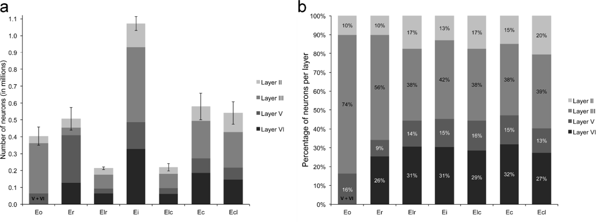
Numbers of neurons in the different layers of the seven subdivisions of the rhesus monkey entorhinal cortex (a). Percentage of neurons contained in each layer, per subdivision (b). See also Table 2.

In light of the variations in the number of neurons located in the different layers of the seven subdivisions of the rhesus monkey entorhinal cortex, it is interesting to consider the ratio between the number of neurons located in the superficial layers II and III, which originate the main feedforward projections toward the dentate gyrus and the hippocampus, and the number of neurons located in the deep layers V and VI, which represent the main recipient of the feedback projections originating in the hippocampus and the subiculum (Figure 5a). This ratio was greater in the rostral subdivisions (Eo and Er) than in all the other subdivisions (F_(6,18)=301.761, p<.001, η²_p=.990). There were no differences between Ei, Elr and Elc. Interestingly, the ratio in Ecl was lower than in Eo and Er, but overall higher than in the other subdivisions, in particular area Ec with which it is often associated.

Figure 5:

Ratio of the number of neurons in the superficial layers (II and III) and the number of neurons in the deep layers (V and VI) in the seven subdivisions of the rhesus monkey entorhinal cortex (a). Ratio of the number of neurons contained in layer III (projecting to CA1 and the subiculum) and the number of neurons contained in layer II (projecting to the dentate gyrus and CA3). Ratio in rat LEC and MEC calculated from the averages of the number of neurons reported in (Merrill et al., 2001; Mulders et al., 1997) for young adult rats.

Consistent with the poor development of the deep layers of area Eo, there are about five times more neurons in the superficial layers than in the deep layers in this subdivision. In area Er, there are about two times more neurons in the superficial layers than in the deep layers. This suggests that these rostral areas play a much larger role in relaying information to the dentate gyrus and the hippocampus than they do in receiving information that has been processed by the hippocampus. Despite some subtle variations between subdivisions, there are on average only about 25% more neurons in the superficial layers than in the deep layers in the other subdivisions of the entorhinal cortex. Interestingly, the ratios between the number of neurons in the superficial versus deep layers of the monkey entorhinal cortex are significantly higher than in the two main subdivisions of the rat entorhinal cortex (LEC-homologous to the primate rostral entorhinal cortex: 1.14; MEC-homologous to the primate caudal entorhinal cortex: 1.10; Table 3). These findings suggest differences in the degree of reciprocity of the connections between different subdivisions of the monkey entorhinal cortex and the rest of the hippocampal formation.

Table 3:

Number of neurons in the different layers of the entorhinal cortex in rats and humans

	Layer II		Layer III		Layer V + VI		All layers
	Mean	SD	Mean	SD	Mean	SD	Mean	SD
Rat MEC	62,924		140,541		184,625		388,090
1	66,400	10,383	128,200	16,423	185,400	24,419	380,000	36,871
2	59,448	8,575	152,881	15,122	183,849	23,490	396,178	29,223
Rat LEC	40,896		112,335		134,546		287,777
1	45,600	13,278	119,400	15,502	143,800	29,575	308,800	44,673
2	36,192	6,133	105,269	18,538	125,291	24,120	266,752	31,034
Rat EC	103,820		252,875		319,170		675,865
1	112,000	22,327	247,600	22,843	329,200	53,844	688,800	76,594
2	95,640	10,543	258,150	23,294	309,140	33,668	663,000	46,000
Monkey EC	499,784	64,505	1,621,012	102,823	1,411,615	145,832	3,532,411	252,997
Human EC	652,500		3,590,500		3,247,500		7,490,500
3	647,000	143,066	3,525,000	623,810	2,711,000	619,757	6,883,000	1,136,076
4	658,000	107,098	3,656,000	570,640	3,784,000	288,929	8,098,000	875,825

¹Mulders et al., 1997. The Journal of Comparative Neurology, 385:83–94.

²Merrill et al., 2001. The Journal of Comparative Neurology, 438:445–456.

³Gomez-Isla et al.,1996. Journal of Neuroscience, 16(14):4491–4500.

⁴West and Slomianka, 1998. Hippocampus, 8:69–82 + 8:426 corrigendum.

It is also interesting to consider the ratio between the number of neurons located in layer III, which originate the projections to CA1 and the subiculum, and the number of neurons located in layer II, which originate the projections to the dentate gyrus and CA3, in order to assess the relative importance of the direct and indirect projections to the hippocampus originating from different subdivisions of the entorhinal cortex (Figure 5b). This ratio was greater in the rostral subdivisions (Eo and Er) than in all the other subdivisions (F_(6,18)=29.042, p<.001, η²_p=.906, Fisher LSD, all p < 0.05). Note, moreover, that the difference between Er and Ei just failed to reach significance, whereas this ratio was higher in Ec than Ecl. In area Eo, there are about 7.5 times more neurons in layer III than in layer II. In area Er, there are about six times more neurons in layer III than in layer II. In area Ei, there are about three times more neurons in layer III than in layer II. Finally, there are between 2 and 2.5 times more neurons in layer III than in layer II in the remaining subdivisions of the rhesus monkey entorhinal cortex. These estimates reveal a clear rostrocaudal gradient, with a relatively greater development of layer III, as compared to layer II, in the rostral entorhinal cortex. Although less prominent, there is a similar pattern in the rat entorhinal cortex, with 2.75 times more neurons in layer III than in layer II in LEC, and only 2.23 times more neurons in layer III than in layer II in MEC.

Neuronal soma size

In addition to the distinct patterns of connectivity described previously, and the differences in the relative number of neurons in the different layers of the seven subdivisions of the rhesus monkey entorhinal cortex shown here, we also found differences in the volume of neuronal somas between subdivisions (Table 2).

• Layer II:

  The average soma volume of layer II neurons differed between subdivisions (F_(6,18)=43.751, p < 0.001, η²_p=.936). Layer II neurons were smaller in area Eo than in all other subdivisions. Layer II neurons were also smaller in area Er than in more caudal subdivisions, but not area Elr (Eo < all other fields; Er < Ei, Elc, Ec, Ecl: all p < 0.05).

• Layer III:

  Although the average soma volume of layer III neurons also differed between subdivisions (F_(6,18)=3.083, p = 0.030, η²_p =.507), these differences were not as pronounced as for layer II neurons. Layer III neurons were smaller in Eo than in Ecl; they were larger in Ei than in Elc.

• Layer V:

  The average soma volume of layer V neurons also differed between subdivisions (F_(6,18)=5.822, p = 0.002, η²_p=.660). Layer V neurons were smaller in area Eo, as compared to all other areas, except for Ecl. Layer V neurons were larger in area Er than in areas Eo, Elr, Elc. Similarly, layer V neurons were larger in area Ei than in areas Eo and Ec.

• Layer VI:

  The average volume of layer VI neurons also differed between subdivisions (F_(6,18)=4.256, p = 0.008, η²_p =.587). Layer VI neurons were larger in Ei than in Elc, Ec and Ecl. They were also larger in area Er than in area Elc. No other differences were statistically significant.

DISCUSSION

Comparison with previous studies

Monkeys

The current study provides normative data on the volume, neuron number and neuronal soma size in the different layers of the seven subdivisions of the adult rhesus monkey entorhinal cortex. To our knowledge, there are only two previous studies that provided partial analyses of neuron number and/or neuronal soma size in the rhesus monkey entorhinal cortex.

Gazzaley et al. (1997) reported a preserved number of entorhinal cortex layer II neurons in aged (24–29-year-old) macaque monkeys, as compared to young adult (7.5–12-year-old) and juvenile (1.2–2-year-old) monkeys. Gazzaley et al. subdivided the entorhinal cortex following the description by Van Hoesen and Pandya (1975). Their counts included the entire rostral and intermediate subdivisions, as well as the caudal subdivision that contained a visible lamina dissecans. As we have reported in our detailed description of the cytoarchitectonic organization of the rhesus monkey entorhinal cortex, the presence of a visible lamina dissecans by itself does not constitute a reliable criterion by which to delineate its different subdivisions. Moreover, in their study, Gazzaley and colleagues first cut the brains into 5–6-mm- thick blocks, prior to cutting coronal sections at 40 μm with a sliding microtome. This procedure necessarily leads to tissue loss with a resulting underestimation of total neuron numbers. Finally, the stereological parameters used to calculate neuron numbers, in particular the thickness of the processed sections and the height of the disector were not reported adequately, and detailed records of the study are no longer available (A. H. Gazzaley, J. H. Morrison and P. R. Hof; pers. comm.). Given these uncertainties, it is difficult to compare the results in Gazzaley et al. (1997) with the current findings.

Merrill et al. (2000) also reported the conservation of neuron number and neuronal soma size in layers II, III and V/VI in the intermediate division of the aged rhesus monkey entorhinal cortex. Their estimates correspond to about half the values we found for the intermediate division Ei in the current study. Inter-laboratory differences may be related to the calibration of the computer-aided analysis systems or other methodological differences that are difficult to identify (Altemus, Lavenex, Ishizuka, & Amaral, 2005). In their study, Merrill et al. cut the brains on a freezing microtome set at 40 μm and reported an average thickness of the Nissl-stained histological sections of about 21 μm. In our study, we cut the brains on a freezing microtome at 60 μm for the Nissl series, and measured an average thickness of Nissl-stained sections of 13.32 μm across all regions/layers. However, since the optical fractionator provides estimates of neuron numbers that are independent of volume measurements, and that the formula used to calculate neuron numbers includes the thickness sampling fraction, it is unclear how such differences in tissue processing may lead to differences in neuron numbers. We are confident regarding the measurement of the thickness of the sections used in the current study, since our computer-aided analysis system is equipped with a Focus Encoder providing 0.1 μm resolution measurements of the actual position of the microscope stage in the z-axis, and does not rely on the pre-defined settings of the motorized stage. The average section thickness measured in the current study is similar to what we previously found during the completion of stereological studies of the rat and monkey amygdala, which have supported the reliability and generalizability of our normative data (Chareyron et al., 2011) and that were very close to those reported by other laboratories (Berdel, Morys, & Maciejewska, 1997; Carlo, Stefanacci, Semendeferi, & Stevens, 2010; Cooke, Stokas, & Woolley, 2007; Rubinow & Juraska, 2009). In our study, the disector height (5 μm) represented 37.5% of the averaged section thickness, the counting frame was 40 μm × 40 μm and we used different scan grids for individual layers (Table 1). In their study, Merrill and colleagues reported counting neurons in the middle 75% of total tissue thickness for each section, with the optical disector dimensions set at 50 μm² (which may have been 50 μm × 50 μm, M. Tuszynski, pers. comm.). However, there was no information about the scan grid size or the total number of neurons counted, which would enable us to recalculate the estimates of neuron numbers, and detailed records of the study are no longer available (D. A. Merrill and M. H. Tuszynski, pers. comm.). Given these uncertainties, it is difficult to compare the results in Merrill et al. (2000) with the current findings.

Interspecies comparisons

Previous comparisons of the structure of the entorhinal cortex in different species have emphasized either the conservation of the general functional organization of the entorhinal cortex across species (Insausti et al., 1997; Naumann et al., 2016; Witter et al., 2017), or the notable differences in the number, relative development and structural characteristics of different subdivisions of the entorhinal cortex between rats, monkeys and humans (Amaral et al., 1987; Amaral & Lavenex, 2007; Insausti et al., 1997; Insausti et al., 1995). Here, we compare the number of neurons in the different layers of the rat, monkey and human entorhinal cortex (Tables 3 and 4). As was the case for the comparison of our current findings with those of previous studies carried out in monkeys, it was difficult to find studies in rats and humans that used reliable, design-based stereological techniques combined with well-accepted delineations of layers and subdivisions of the entorhinal cortex. We considered two studies in rats, our current findings in monkeys, and two studies in humans, in order to compare the relative development and quantitative structural characteristics of the entorhinal cortex in different species.

Table 4:

Number of neurons in the different layers of the entorhinal cortex, in rats, monkeys and humans

	Rat1	Monkey2	Human3	M/R	H/R	H/M
II	103,820	499,784	652,500	4.81	6.28	1.31
III	252,875	1,621,012	3,590,500	6.41	14.20	2.21
V + VI	319,170	1,411,615	3,247,500	4.41	10.17	2.30
Total	675,865	3,532,411	7,490,500	5.23	11.08	2.12
(II+III) / (V+VI)	1.12	1.50	1.31
III / II	2.44	3.24	5.50

¹Average data of studies reported in Table 3

²Data from current study reported in Table 3

³Average data of studies reported in Table 3

Rats:

Mulders et al. (1997) estimated the number of neurons in the different layers of the lateral and medial entorhinal cortex of 30-day-old female Wistar rats. Merrill et al. (2001) estimated the number of neurons in the lateral and medial entorhinal cortex in 2-month-old female Fischer 344 rats (they also reported data on 21-month-old rats, which we did not include in Table 3). The results of these two studies, carried out in two independent laboratories, provide consistent estimates.

Humans:

Gomez-Isla et al. (1996) estimated the number of neurons in the entire entorhinal cortex of non-demented men and women between 60 and 89 years of age. Note that the definitions of the layers reported in their study differed from that used in other studies, so we adapted the presentation of their results to match the definitions used in the other studies. West and Slomianka (West & Slomianka, 1998a, 1998b) estimated the number of neurons in the entire entorhinal cortex of 19–58-year-old men. The results of these two studies, carried out in two independent laboratories, provided consistent estimates of the number of neurons in layers II and III. In contrast, there was a relatively larger difference between studies in their estimates of the number of neurons in layers V and VI. Nevertheless, these estimates can be considered sufficiently reliable to perform interspecies comparisons of the relative number of neurons in different layers of the entorhinal cortex.

Since the previous studies in rats or humans did not report the number of neurons in the different subdivisions of the entorhinal cortex based on the nomenclature defined by Amaral and colleagues for monkeys (Amaral et al., 1987), Insausti and colleagues for humans (Insausti et al., 1995) and rats (Insausti et al., 1997), we limit our species comparisons to the number of neurons in the entire entorhinal cortex (Tables 3 and 4). We consider layer II neurons as the origin of the entorhinal cortex projections to the dentate gyrus and CA3; layer III neurons as the origin of the entorhinal cortex projections to CA1 and the subiculum; and layer V and VI neurons as the main layers of the entorhinal cortex receiving the hippocampal output projections originating in CA1 and the subiculum.

As compared to rats, the total number of neurons in the entorhinal cortex is about 5 times greater in monkeys, and 11 times greater in humans (and thus about 2 times greater in humans than in monkeys). In layer II, there are 4.8 times more neurons in monkeys than in rats, 6.3 times more neurons in humans than in rats, and 1.3 times more neurons in humans than in monkeys. In layer III, there are 6.4 times more neurons in monkeys than in rats, 14.2 times more neurons in humans than in rats, and 2.2 times more neurons in humans than in monkeys. In layer V and VI, there are 4.4 times more neurons in monkeys than in rats, 10.2 times more neurons in humans than in rats, and 2.3 times more neurons in humans than in monkeys. These findings suggest that the relative importance of the different inputs to the hippocampal formation (via entorhinal cortex layer II and layer III neurons, respectively) may vary between species. Specifically, the ratio between the number of neurons in layer III and the number of neurons in layer II is 2.4 in rats, 3.2 in monkeys, and 5.5 in humans. Thus, the direct entorhinal cortex projection to CA1 appears greater in primates than in rats, and appears further developed in humans as compared to monkeys. Interestingly, the ratio between the number of neurons in the superficial layers and the number of neurons in the deep layers appears greater in monkeys and humans than in rats (Table 4). This pattern may be related to the greater development of the neocortical areas projecting to the superficial layers of the entorhinal cortex in primates. This finding is similar to what we observed previously for different amygdala nuclei (Chareyron et al., 2011), and consistent with the theory that brain structures with major anatomical and functional links evolve together independently of evolutionary changes in other unrelated structures (Barton & Harvey, 2000).

In sum, our detailed analysis of neuron numbers and neuronal soma size in the different layers of distinct subdivisions of the monkey entorhinal cortex confirms that the entorhinal cortex is a very heterogeneous structure and that interspecies comparisons should take into account these important regional differences. Our data further suggest that, despite being consistent with functional studies in rodents and connectional studies in monkeys, a simple parcellation of the primate entorhinal cortex into two major functional subregions, homologous to the rodent LEC and MEC (Maass et al., 2015; Navarro Schroder et al., 2015; Reagh et al., 2018), may be too simplistic to capture the full complexity of information processing carried out by the human entorhinal cortex. The development of comprehensive high-resolution atlases of the human brain based on the microscopic evaluation of histological sections (Ding et al., 2017) may contribute to reach that goal. We will now focus on our findings in monkeys, in order to discuss the possible functional implications of the relative development of the different layers in the different subdivisions of the primate entorhinal cortex.

Different entorhinal-hipppocampal circuits

As was previously recognized from connectional studies and cytoarchitectural descriptions, the quantitative estimates of neuron numbers and descriptions of morphological characteristics reported here emphasize the heterogeneity of the entorhinal cortex, even within a single species.

Area Eo:

Although area Eo can be distinguished based on several cytoarchitectonic features, it was named based on the fact that in monkeys it is the only region of the entorhinal cortex that receives a direct input from the olfactory bulb. This input is unique in being unimodal and coming from a very early stage of olfactory sensory processing. It is thus interesting to consider that there are five times more neurons in the superficial layers than in the deep layers of Eo, and that there are about 7.5 times more neurons in layer III than in layer II. One can thus surmise that, in primates, the olfactory input from the olfactory bulb is mostly transmitted via direct projections from layer III neurons to the rostral portion of CA1 (Insausti, Marcos, Arroyo-Jimenez, Blaizot, & Martinez-Marcos, 2002). In turn, hippocampal output may have a rather limited influence on information processing taking place in area Eo.

Areas Er and Elr:

Area Er receives the majority of its cortical afferents from the perirhinal cortex, which projects mainly to the rostral two thirds of the entorhinal cortex (areas Eo, Er, Elr, Elc, Ei) (Suzuki & Amaral, 1994b). Interestingly, the degree of reciprocity of the projections between the perirhinal cortex and the entorhinal cortex appears to vary depending on the region of the entorhinal cortex examined. Projections between the perirhinal cortex and the lateral portions of the entorhinal cortex (including area Elr) are more reciprocal than the projections with the medial portions of the entorhinal cortex. Projections from cells in layer III of the perirhinal cortex terminate most strongly in layers I, II and the superficial portion of layer III of the entorhinal cortex. Consistent with the fact that the projection from the entorhinal cortex to the perirhinal cortex originates mainly from cells situated in layer V (with only very few cells located in layers VI and III), the ratio between the number of neurons in the superficial layers and the number of neurons in the deep layers is higher for area Er than for area Elr. These findings are consistent with the observation that the connections between the perirhinal cortex and area Elr are more reciprocal than with area Er (an area sending relatively fewer feedback projections to the perirhinal cortex) (Suzuki & Amaral, 1994b).

Area Ei and Elc:

Area Ei is defined as the intermediate subdivision of the entorhinal cortex and shares some structural and functional characteristics with both the rostral and caudal subdivisions of the entorhinal cortex. Ei receives prominent projections from the perirhinal cortex, which reach the rostral two thirds of the entorhinal cortex, and projections from the parahippocampal cortex, which reach the caudal two thirds of the entorhinal cortex. Interestingly, the ratio between the number of neurons in the superficial layers and the number of neurons in the deep layers is lower in areas Ei and Elc than in rostral areas Er and Eo, and is similar to that found in area Elr and caudal areas Ec and Ecl. It thus seems consistent that highly reciprocal projections between the parahippocampal cortex and the entorhinal cortex are associated with a higher number of neurons in layer V in the subdivisions of the entorhinal cortex that originate the majority of these projections (Suzuki & Amaral, 1994b).

Areas Ec and Ecl:

Areas Ec and Ecl receive prominent projections from layer III neurons in the parahippocampal cortex, which terminate most strongly in layers I, II and III. In addition, areas Ec and Ecl are characterized by a direct projection from the presubiculum to layer III. Interestingly, this connection is also a defining feature of the rat medial entorhinal cortex (MEC), which is particularly involved in spatial information processing (Knierim et al., 2014; Witter & Moser, 2006). The connections between these two areas and the parahippocampal cortex are highly reciprocal (Suzuki & Amaral, 1994b), which appears to be also reflected in the lower ratio between the number of neurons in the superficial layers and the number of neurons in the deep layers, as compared to the rostral subdivisions Er and Eo. However, this ratio was slightly higher in Ecl than in Ec, whereas the ratio between the number of neurons in layer III (projecting to CA1 and the subiculum) and the number of neurons in layer II (projecting to the dentate gyrus and CA3) was slightly higher in Ec than Ecl. Thus, although these two areas share some common connectional characteristics (Amaral & Lavenex, 2007; Suzuki & Amaral, 1994b) and functional properties (Chareyron et al., 2017), they nevertheless differ in the relative numbers of neurons contributing to different hippocampal circuits. Although areas Ec and Ecl represent approximately the same percentage of the volume of the entire entorhinal cortex, and contain about the same percentage of all the neurons in the entire entorhinal cortex, area Ec contains a proportionally larger number of neurons in layer II, which are known to contribute projections to the dentate gyrus and CA3. The functional consequences of such differences remain to be determined.

CONCLUSION

This study provides normative data on the volume, neuron number and neuronal soma size in the different layers of the seven subdivisions of the rhesus monkey entorhinal cortex. These data corroborate the important structural differences between different subdivisions of the monkey entorhinal cortex. In particular, differences in the number of neurons contributing to distinct afferent and efferent hippocampal pathways suggest not only that different types of information may be more or less segregated between caudal and rostral subdivisions, but also, and perhaps most importantly, that the nature of the interaction between the entorhinal cortex and the rest of the hippocampal formation may vary between different subdivisions. Finally, these data provide fundamental information on the number of functional units that comprise the entorhinal-hippocampal circuits and should be considered in order to build more realistic models of the human medial temporal lobe memory system.

Figure 2b:

High magnification photomicrographs of coronal sections through the adult rhesus monkey entorhinal cortex. g-j. Nissl-stained preparations. k-n. SMI-32 immunohistochemistry). g and k. Ei, intermediate field; h and l. Elc, lateral caudal field; i and m. Ec, caudal field; j and n. Ecl, caudal limiting field. Scale bar = 250 μm.

REFERENCES

- Altemus KL, Lavenex P, Ishizuka N, & Amaral DG (2005). Morphological characteristics and electrophysiological properties of CA1 pyramidal neurons in macaque monkeys. Neuroscience, 136(3), 741–756. doi: 10.1016/j.neuroscience.2005.07.001 [DOI] [PubMed] [Google Scholar]
- Amaral DG, Insausti R, & Cowan WM (1987). The entorhinal cortex of the monkey: I. Cytoarchitectonic organization. J Comp Neurol, 264(3), 326–355. [DOI] [PubMed] [Google Scholar]
- Amaral DG, Kondo H, & Lavenex P (2014). An analysis of entorhinal cortex projections to the dentate gyrus, hippocampus, and subiculum of the neonatal macaque monkey. J Comp Neurol, 522(7), 1485–1505. doi: 10.1002/cne.23469 [DOI] [PMC free article] [PubMed] [Google Scholar]
- Amaral DG, & Lavenex P (2007). Hippocampal neuroanatomy In Andersen P, Morris RGM, Amaral DG, Bliss TV, & O’Keefe J (Eds.), The hippocampus book (pp. 37–114). Oxford: Oxford University Press. [Google Scholar]
- Amaral DG, & Witter MP (2003). The entorhinal cortex of the monkey: VI. Organization of projections from the hippocampus and subicular complex. Journal of Comparative Neurology, Submitted. [DOI] [PubMed] [Google Scholar]
- Barton RA, & Harvey PH (2000). Mosaic evolution of brain structure in mammals. Nature, 405(6790), 1055–1058. doi: 10.1038/35016580 [DOI] [PubMed] [Google Scholar]
- Berdel B, Morys J, & Maciejewska B (1997). Neuronal changes in the basolateral complex during development of the amygdala of the rat. Int J Dev Neurosci, 15(6), 755–765. [DOI] [PubMed] [Google Scholar]
- Carlo CN, Stefanacci L, Semendeferi K, & Stevens CF (2010). Comparative analyses of the neuron numbers and volumes of the amygdaloid complex in old and new world primates. J Comp Neurol, 518(8), 1176–1198. doi: 10.1002/cne.22264 [DOI] [PubMed] [Google Scholar]
- Chareyron LJ, Banta Lavenex P, Amaral DG, & Lavenex P (2011). Stereological analysis of the rat and monkey amygdala. J Comp Neurol, 519(16), 3218–3239. doi: 10.1002/cne.22677 [DOI] [PMC free article] [PubMed] [Google Scholar]
- Chareyron LJ, Banta Lavenex P, Amaral DG, & Lavenex P (2012). Postnatal development of the amygdala: A stereological study in macaque monkeys. J Comp Neurol, 520(9), 1965–1984. doi: 10.1002/cne.23023 [DOI] [PMC free article] [PubMed] [Google Scholar]
- Chareyron LJ, Banta Lavenex P, Amaral DG, & Lavenex P (2017). Functional organization of the medial temporal lobe memory system following neonatal hippocampal lesion in rhesus monkeys. Brain Struct Funct. doi: 10.1007/s00429-017-1441-z [DOI] [PMC free article] [PubMed] [Google Scholar]
- Chrobak JJ, & Amaral DG (2007). Entorhinal cortex of the monkey: VII. intrinsic connections. J Comp Neurol, 500(4), 612–633. doi: 10.1002/cne.21200 [DOI] [PubMed] [Google Scholar]
- Cooke BM, Stokas MR, & Woolley CS (2007). Morphological sex differences and laterality in the prepubertal medial amygdala. J Comp Neurol, 501(6), 904–915. doi: 10.1002/cne.21281 [DOI] [PubMed] [Google Scholar]
- de Haas Ratzliff A, & Soltesz I (2000). Differential expression of cytoskeletal proteins in the dendrites of parvalbumin-positive interneurons versus granule cells in the adult rat dentate gyrus. Hippocampus, 10(2), 162–168. [PubMed] [Google Scholar]
- Ding SL, Royall JJ, Sunkin SM, Ng L, Facer BA, Lesnar P, … LeinReference ES (2017). Comprehensive cellular-resolution atlas of the adult human brain. J Comp Neurol, 525(2), 407. doi: 10.1002/cne.24130 [DOI] [PMC free article] [PubMed] [Google Scholar]
- Fitting S, Booze RM, Hasselrot U, & Mactutus CF (2008). Differential long-term neurotoxicity of HIV-1 proteins in the rat hippocampal formation: a design-based stereological study. Hippocampus, 18(2), 135–147. doi: 10.1002/hipo.20376 [DOI] [PMC free article] [PubMed] [Google Scholar]
- Gazzaley AH, Thakker MM, Hof PR, & Morrison JH (1997). Preserved number of entorhinal cortex layer II neurons in aged macaque monkeys. Neurobiol Aging, 18(5), 549–553. [DOI] [PubMed] [Google Scholar]
- Goldstein ME, Sternberger LA, & Sternberger NH (1987). Varying degrees of phosphorylation determine microheterogeneity of the heavy neurofilament polypeptide (NF-H). J. Neuroimmunol, 14, 135–148. [DOI] [PubMed] [Google Scholar]
- Gomez-Isla T, Price JL, McKeel DW Jr., Morris JC, Growdon JH, & Hyman BT (1996). Profound loss of layer II entorhinal cortex neurons occurs in very mild Alzheimer’s disease. J Neurosci, 16(14), 4491–4500. [DOI] [PMC free article] [PubMed] [Google Scholar]
- Grady MS, Charleston JS, Maris D, Witgen BM, & Lifshitz J (2003). Neuronal and glial cell number in the hippocampus after experimental traumatic brain injury: analysis by stereological estimation. J Neurotrauma, 20(10), 929–941. doi: 10.1089/089771503770195786 [DOI] [PubMed] [Google Scholar]
- Gundersen HJ (1988). The nucleator. J Microsc, 151(Pt 1), 3–21. [DOI] [PubMed] [Google Scholar]
- Hamidi M, Drevets WC, & Price JL (2004). Glial reduction in amygdala in major depressive disorder is due to oligodendrocytes. Biol Psychiatry, 55(6), 563–569. doi: 10.1016/j.biopsych.2003.11.006 [DOI] [PubMed] [Google Scholar]
- Hof PR, & Morrison JH (1995). Neurofilament protein defines regional patterns of cortical organization in the macaque monkey visual system: a quantitative immunohistochemical analysis. J Comp Neurol, 352(2), 161–186. doi: 10.1002/cne.903520202 [DOI] [PubMed] [Google Scholar]
- Hornung JP, & Riederer BM (1999). Medium-sized neurofilament protein related to maturation of a subset of cortical neurons. J Comp Neurol, 414(3), 348–360. doi: 10.1002/(SICI)1096-9861(19991122)414:3<348::AID-CNE5>3.0.CO;2-H [pii] [DOI] [PubMed] [Google Scholar]
- Insausti R, Amaral DG, & Cowan WM (1987). The entorhinal cortex of the monkey: II. Cortical afferents. J Comp Neurol, 264(3), 356–395. [DOI] [PubMed] [Google Scholar]
- Insausti R, Herrero MT, & Witter MP (1997). Entorhinal cortex of the rat: cytoarchitectonic subdivisions and the origin and distribution of cortical efferents. Hippocampus, 7(2), 146–183. doi: 10.1002/(SICI)1098-1063(1997)7:2<146::AID-HIPO4>3.0.CO;2-L [DOI] [PubMed] [Google Scholar]
- Insausti R, Marcos P, Arroyo-Jimenez MM, Blaizot X, & Martinez-Marcos A (2002). Comparative aspects of the olfactory portion of the entorhinal cortex and its projection to the hippocampus in rodents, nonhuman primates, and the human brain. Brain Res Bull, 57(3–4), 557–560. [DOI] [PubMed] [Google Scholar]
- Insausti R, Tunon T, Sobreviela T, Insausti AM, & Gonzalo LM (1995). The human entorhinal cortex: a cytoarchitectonic analysis. J Comp Neurol, 355(2), 171–198. doi: 10.1002/cne.903550203 [DOI] [PubMed] [Google Scholar]
- Jabes A, Banta Lavenex P, Amaral DG, & Lavenex P (2010). Quantitative analysis of postnatal neurogenesis and neuron number in the macaque monkey dentate gyrus. Eur J Neurosci, 31(2), 273–285. doi: 10.1111/j.1460-9568.2009.07061.x [DOI] [PMC free article] [PubMed] [Google Scholar]
- Jabes A, Banta Lavenex P, Amaral DG, & Lavenex P (2011). Postnatal development of the hippocampal formation: a stereological study in macaque monkeys. J Comp Neurol, 519(6), 1051–1070. doi: 10.1002/cne.22549 [DOI] [PMC free article] [PubMed] [Google Scholar]
- Knierim JJ, Neunuebel JP, & Deshmukh SS (2014). Functional correlates of the lateral and medial entorhinal cortex: objects, path integration and local-global reference frames. Philos Trans R Soc Lond B Biol Sci, 369(1635), 20130369. doi: 10.1098/rstb.2013.0369 [DOI] [PMC free article] [PubMed] [Google Scholar]
- Lavenex P, & Amaral DG (2000). Hippocampal-neocortical interaction: a hierarchy of associativity. Hippocampus, 10(4), 420–430. doi: 10.1002/1098-1063(2000)10:4<420::AID-HIPO8>3.0.CO;2-5 [DOI] [PubMed] [Google Scholar]
- Lavenex P, Banta Lavenex P, & Amaral DG (2004). Nonphosphorylated high-molecular-weight neurofilament expression suggests early maturation of the monkey subiculum. Hippocampus, 14(7), 797–801. doi: 10.1002/hipo.20028 [DOI] [PubMed] [Google Scholar]
- Lavenex P, Banta Lavenex P, Bennett JL, & Amaral DG (2009). Postmortem changes in the neuroanatomical characteristics of the primate brain: hippocampal formation. J Comp Neurol, 512(1), 27–51. doi: 10.1002/cne.21906 [DOI] [PMC free article] [PubMed] [Google Scholar]
- Maass A, Berron D, Libby LA, Ranganath C, & Duzel E (2015). Functional subregions of the human entorhinal cortex. Elife, 4. doi: 10.7554/eLife.06426 [DOI] [PMC free article] [PubMed] [Google Scholar]
- Merrill DA, Chiba AA, & Tuszynski MH (2001). Conservation of neuronal number and size in the entorhinal cortex of behaviorally characterized aged rats. J Comp Neurol, 438(4), 445–456. [DOI] [PubMed] [Google Scholar]
- Merrill DA, Roberts JA, & Tuszynski MH (2000). Conservation of neuron number and size in entorhinal cortex layers II, III, and V/VI of aged primates. J Comp Neurol, 422(3), 396–401. [DOI] [PubMed] [Google Scholar]
- Morris JA, Jordan CL, & Breedlove SM (2008). Sexual dimorphism in neuronal number of the posterodorsal medial amygdala is independent of circulating androgens and regional volume in adult rats. J Comp Neurol, 506(5), 851–859. doi: 10.1002/cne.21536 [DOI] [PubMed] [Google Scholar]
- Mulders WH, West MJ, & Slomianka L (1997). Neuron numbers in the presubiculum, parasubiculum, and entorhinal area of the rat. J Comp Neurol, 385(1), 83–94. [PubMed] [Google Scholar]
- Naumann RK, Ray S, Prokop S, Las L, Heppner FL, & Brecht M (2016). Conserved size and periodicity of pyramidal patches in layer 2 of medial/caudal entorhinal cortex. J Comp Neurol, 524(4), 783–806. doi: 10.1002/cne.23865 [DOI] [PMC free article] [PubMed] [Google Scholar]
- Navarro Schroder T, Haak KV, Zaragoza Jimenez NI, Beckmann CF, & Doeller CF (2015). Functional topography of the human entorhinal cortex. Elife, 4. doi: 10.7554/eLife.06738 [DOI] [PMC free article] [PubMed] [Google Scholar]
- Palackal T, Neuringer M, & Sturman J (1993). Laminar analysis of the number of neurons, astrocytes, oligodendrocytes and microglia in the visual cortex (area 17) of 6- and 12-month-old rhesus monkeys fed a human infant soy-protein formula with or without taurine supplementation from birth. Dev Neurosci, 15(1), 54–67. doi: 10.1159/000111317 [DOI] [PubMed] [Google Scholar]
- Pitkänen A, Kelly JL, & Amaral DG (2002). Projections from the lateral, basal, and accessory basal nuclei of the amygdala to the entorhinal cortex in the macaque monkey. Hippocampus, 12(2), 186–205. [DOI] [PubMed] [Google Scholar]
- Reagh ZM, Noche JA, Tustison NJ, Delisle D, Murray EA, & Yassa MA (2018). Functional Imbalance of Anterolateral Entorhinal Cortex and Hippocampal Dentate/CA3 Underlies Age-Related Object Pattern Separation Deficits. Neuron, 97(5), 1187–1198 e1184. doi: 10.1016/j.neuron.2018.01.039 [DOI] [PMC free article] [PubMed] [Google Scholar]
- Rubinow MJ, & Juraska JM (2009). Neuron and glia numbers in the basolateral nucleus of the amygdala from preweaning through old age in male and female rats: a stereological study. J Comp Neurol, 512(6), 717–725. doi: 10.1002/cne.21924 [DOI] [PMC free article] [PubMed] [Google Scholar]
- Siegel SJ, Ginsberg SD, Hof PR, Foote SL, Young WG, Kraemer GW, … Morrison JH (1993). Effects of social deprivation in prepubescent rhesus monkeys: immunohistochemical analysis of the neurofilament protein triplet in the hippocampal formation. Brain Res, 619(1–2), 299–305. doi:0006–8993(93)91624–2 [pii] [DOI] [PubMed] [Google Scholar]
- Sternberger LA, & Sternberger NH (1983). Monoclonal antibodies distinguish phosphorylated and nonphosphorylated forms of neurofilaments in situ. Proc Natl Acad Sci U S A, 80(19), 6126–6130. [DOI] [PMC free article] [PubMed] [Google Scholar]
- Suzuki WA, & Amaral DG (1994a). Perirhinal and parahippocampal cortices of the macaque monkey: cortical afferents. J Comp Neurol, 350, 497–533. [DOI] [PubMed] [Google Scholar]
- Suzuki WA, & Amaral DG (1994b). Topographic organization of the reciprocal connections between the monkey entorhinal cortex and the perirhinal and parahippocampal cortices. Journal of Neuroscience, 14(3), 1856–1877. [DOI] [PMC free article] [PubMed] [Google Scholar]
- Van Hoesen GW, & Pandya DN (1975). Some connections of the entorhinal (area 28) and perirhinal (area 35) cortices of the rhesus monkey. I. Temporal lobe afferents. Brain Research, 95(1), 1–24. [DOI] [PubMed] [Google Scholar]
- van Strien NM, Cappaert NL, & Witter MP (2009). The anatomy of memory: an interactive overview of the parahippocampal-hippocampal network. Nat Rev Neurosci, 10(4), 272–282. doi: 10.1038/nrn2614 [DOI] [PubMed] [Google Scholar]
- West MJ, & Slomianka L (1998a). Total number of neurons in the layers of the human entorhinal cortex. Hippocampus, 8(1), 69–82. doi: 10.1002/(SICI)1098-1063(1998)8:1<69::AID-HIPO7>3.0.CO;2-2 [DOI] [PubMed] [Google Scholar]
- West MJ, & Slomianka L (1998b). West MJ, Slomianka L. Total Numbers of Neurons in the Layers of the Human Entorhinal Cortex. Hippocampus 1998;8:69–82. Hippocampus, 8, 426. [DOI] [PubMed] [Google Scholar]
- West MJ, Slomianka L, & Gundersen HJ (1991). Unbiased stereological estimation of the total number of neurons in thesubdivisions of the rat hippocampus using the optical fractionator. Anat Rec, 231(4), 482–497. [DOI] [PubMed] [Google Scholar]
- Witter MP, & Amaral DG (1991). Entorhinal cortex of the monkey: V. Projections to the dentate gyrus, hippocampus, and subicular complex. J Comp Neurol, 307(3), 437–459. [DOI] [PubMed] [Google Scholar]
- Witter MP, Doan TP, Jacobsen B, Nilssen ES, & Ohara S (2017). Architecture of the entorhinal cortex: A review of entorhinal anatomy in rodents with some comparative perspective. Frontiers in Systems Neuroscience, 11. doi:doi: 10.3389/fnsys.2017.00046 [DOI] [PMC free article] [PubMed] [Google Scholar]
- Witter MP, & Moser EI (2006). Spatial representation and the architecture of the entorhinal cortex. Trends Neurosci, 29(12), 671–678. doi: 10.1016/j.tins.2006.10.003 [DOI] [PubMed] [Google Scholar]
- Witter MP, Van Hoesen GW, & Amaral DG (1989). Topographical organization of the entorhinal projection to the dentate gyrus of the monkey. Journal of Neuroscience, 9(1), 216–228. [DOI] [PMC free article] [PubMed] [Google Scholar]