Power analysis in a SMART design: sample size estimation for determining the best embedded dynamic treatment regime

Summary

Sequential, multiple assignment, randomized trial (SMART) designs have become increasingly popular in the field of precision medicine by providing a means for comparing more than two sequences of treatments tailored to the individual patient, i.e., dynamic treatment regime (DTR). The construction of evidence-based DTRs promises a replacement to ad hoc one-size-fits-all decisions pervasive in patient care. However, there are substantial statistical challenges in sizing SMART designs due to the correlation structure between the DTRs embedded in the design (EDTR). Since a primary goal of SMARTs is the construction of an optimal EDTR, investigators are interested in sizing SMARTs based on the ability to screen out EDTRs inferior to the optimal EDTR by a given amount which cannot be done using existing methods. In this article, we fill this gap by developing a rigorous power analysis framework that leverages the multiple comparisons with the best methodology. Our method employs Monte Carlo simulation to compute the number of individuals to enroll in an arbitrary SMART. We evaluate our method through extensive simulation studies. We illustrate our method by retrospectively computing the power in the Extending Treatment Effectiveness of Naltrexone (EXTEND) trial. An R package implementing our methodology is available to download from the Comprehensive R Archive Network.

1. Introduction

Sequential, multiple assignment, randomized trial (SMART) designs have gained considerable attention in the field of precision medicine by providing an empirically rigorous experimental approach for comparing more than two sequences of treatments tailored to the individual patient, i.e., dynamic treatment regime (DTR) (Lavori and others, 2000; Murphy, 2005; Lei and others, 2012). A DTR is a treatment algorithm implemented through a sequence of decision rules which dynamically adjusts treatments and dosages to a patient’s unique changing need and circumstances (Murphy and others, 2001; Murphy, 2003; Robins, 2004; Nahum-Shani and others, 2012; Chakraborty and Moodie, 2013; Chakraborty and Murphy, 2014; Laber and others, 2014). SMARTs are motivated by scientific questions concerning the construction of an effective DTR. The sequential randomization in a SMART gives rise to several DTRs which are embedded in the SMART by design (EDTR). Many SMARTs are designed to compare more than two EDTRs and identify those showing greatest potential for improving a primary clinical outcome. The construction of evidence-based EDTRs promises an alternative to ad hoc one-size-fits-all decisions pervasive in patient care (Chakraborty, 2011).

The advent of SMART designs poses interesting statistical challenges in the planning phase of the trials. In particular, determining an appropriate sample size of individuals to enroll becomes analytically difficult due to the correlation structure between the EDTRs. Previous work includes sizing pilot SMARTs (small scale versions of a SMART) so that each sequence of treatments has a pre-specified number of individuals with some probability by the end of the trial (Almirall and others, 2012; Gunlicks-Stoessel and others, 2016; Kim and others, 2016). The central questions motivating this work are feasibility of the investigators to carry out the trial and acceptability of the treatments by patients. These methods do not provide a means to size SMARTs for comparing EDTRs in terms of a primary clinical outcome.

Alternatively, Crivello and others (2007a) proposed a new objective for SMART sample size planning. The question they address is how many individuals need to be enrolled so that the best EDTR has the largest sample estimate with a given probability (Crivello and others, 2007b). Such an approach based on estimation alone fails to account for the fact that some EDTRs may be statistically indistinguishable from the true best EDTR for the given data in which case they should not necessarily be excluded as suboptimal. Our approach goes one step further than Crivello’s by providing a means to size SMARTs in order to construct narrow confidence intervals which not only tell which is the best EDTR, but also provide the ability to screen out inferior EDTRs. Crivello and others (2007a) also discussed sizing SMARTs to attain a specified power for testing hypotheses which compare only two treatments or two EDTRs as opposed to comparing all EDTRs. The work of Crivello and others (2007a) focused mainly on a particular common two-stage SMART design whereas our method is applicable to arbitrary SMART designs.

More recently, Ogbagaber and others (2016) proposed two methods for sizing a SMART. Their first approach is to choose the sample size in order to achieve a specified power for a global chi-squared test of equality of EDTR outcomes. Their second approach is to choose the sample size in order to detect pairwise differences between EDTR outcomes while adjusting for a specified number of pairwise comparisons using the Bonferroni correction. Their second approach sizes a SMART so that for each pairwise comparison, a difference can be detected with a specified probability . Our approach offers an alternative which requires a smaller sample size to achieve the same power.

One of the main goals motivating SMARTs is to identify the optimal EDTR. It follows that investigators are interested in sizing SMARTs based on the ability to screen out EDTRs which are inferior to the optimal EDTR by a clinically meaningful amount while including the best EDTR with a specified probability. In this article, we develop a rigorous power analysis framework that leverages the multiple comparisons with the best (MCB) methodology (Hsu, 1981, 1984, 1996). The main justification for using MCB to adjust for multiple comparisons is that it involves fewer comparisons compared to other methods and thus, it yields greater power for the same sample size with all else being equal (Ertefaie and others, 2015).

In Section 2, we give a brief overview of SMARTs, notation, and background on estimation and MCB. In Section 3, we present our power analysis framework. In Section 4, we look at the sensitivity of the power to the covariance matrix of EDTR outcomes. In Section 5, we demonstrate the validity of our method through extensive simulation studies. In Section 6, we apply our method to retrospectively compute the power in the Extending Treatment Effectiveness of Naltrexone (EXTEND) trial. In Section 7, we discuss how to choose the covariance matrix of EDTR outcomes for sample size calculations. In Sections 8 and 9, we give concluding remarks. In the supplementary material available at Biostatistics online, we provide additional details about our simulation study, a comparison with the method presented in Ogbagaber and others (2016), and additional simulation studies for power analysis when data from a pilot SMART is available. The R package “smartsizer” is available to download from the Comprehensive R Archive Network.

2. Preliminaries

2.1. Sequential multiple assignment randomized trials (SMART)

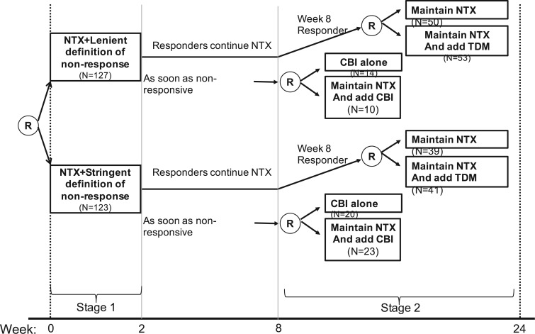
In a SMART, individuals proceed through multiple stages of randomization such that some or all individuals may be randomized more than once. Additionally, treatment assignment is often tailored to the individuals’ ongoing response status (Nahum-Shani and others, 2012). For example, in the Extending Treatment Effectiveness of Naltrexone (EXTEND) trial (see Figure 1 for the study design and Nahum-Shani and others, 2017 for more details about this study), individuals were initially randomized to two different criteria of non-response: lenient or stringent. Specifically, all individuals received the same fixed dosage of naltrexone (NTX)—a medication that blocks some of the pleasurable effects resulting from alcohol consumption. After the first 2 weeks, individuals were evaluated weekly to assess response status. Individuals assigned to the lenient criterion were classified as non-responders as soon as they had five or more heavy drinking days during the first 8 weeks of the study, whereas those assigned to the stringent criterion were classified as non-responders as soon as they had two or more heavy drinking days during the first eight weeks. As soon as participants were classified as non-responders, they transitioned to the second stage where they were randomized to two subsequent rescue tactics: switch to combined behavioral intervention (CBI) or add CBI to NTX (NTX + CBI). At week 8, individuals who did not meet their assigned non-response criterion were classified as responders and re-randomized to two subsequent maintenance interventions: add telephone disease management (TDM) to NTX (NTX + TDM) or continue NTX alone. Note that the stage-2 treatment options in the SMART are tailored to the individuals’ early response status. This leads to a total of eight EDTRs. For example, one of these EDTRs recommends to start the treatment with NTX and monitor drinking behaviors weekly using the lenient criterion (i.e., 5 or more heavy drinking days) to classify the individual as a non-responder. As soon as the individual is classified as a non-responder, add CBI (NTX + CBI); if at week 8 the individual is classified as a responder, add TDM (NTX + TDM). A primary goal motivating many SMARTs is the determination of optimal EDTR. For example, determining an optimal EDTR in the EXTEND may guide in evaluating a patient’s initial response to NTX and in selecting the best subsequent treatment. We develop our power analysis framework with this goal in mind.

Fig. 1.

This diagram shows the structure of the EXTEND trial.

One important challenge for power analysis in SMART designs is the correlation of EDTR outcomes. The correlation arises, in part, due to overlapping interventions in distinct EDTRs and because patients’ treatment histories may be consistent with more than a single EDTR. For example, patients in distinct EDTRs of the EXTEND trial all receive NTX. Also, patients who are classified as responders in stage 2 and subsequently randomized to NTX will be consistent with two EDTRs: one where non-responders are offered CBI and one where non-responders are offered NTX + CBI. In Sections 4 and 5, we will discuss the dependence of power on the covariance. We provide guidelines on choosing the covariance matrix in Section 7.

2.2. Notation

We focus on notation for two-stage SMART designs, but the methods in this paper are applicable to an arbitrary SMART. We use the same notation as in Ertefaie and others (2015). Let and denote the observed covariates and treatment assignment, respectively, at stage . Let and denote the covariate and treatment histories up to and including stage , respectively. Let the treatment trajectory be the vector of counterfactual treatment assignments for an individual. For example, in a two-stage SMART with stage-2 treatment tailored to response status, may be of the form where is the stage-2 treatment assignment had the individual responded and is the stage-2 treatment assignment had the individual not responded. The reason these are counterfactual treatment assignments is that for an individual who responds to the stage-1 treatment, would be unobserved. Hence, the treatment history would be while the treatment trajectory would be and would include the unobserved counterfactual. Let be the embedded tailoring variable for the stage-2 treatment. For example, in EXTEND, is the indicator of response to the stage-1 treatment. Let denotes the continuous observed outcome of an individual at the end of the study. Let the th EDTR be denoted by . Let be the true mean outcome vector of EDTRs where is the total number of EDTRs. Let denote the sample size.

2.3. Estimation

We summarize the estimation procedures inverse probability weighting (IPW) and augmented inverse probability weighting (AIPW) introduced in Ertefaie and others (2015) for a two-stage SMART, but the method can be extended to arbitrary SMART designs. In order to perform estimation with IPW/AIPW, a marginal structural model (MSM) must be specified. A MSM models the response as a function of the counterfactual random treatment assignments in the treatment trajectory vector , while ignoring non-treatment covariates. For example, in a two-stage SMART, a MSM is: Subsequently, the IPW and AIPW estimators and for may be obtained by solving the following respective estimating equations:

(IPW)

(AIPW)

where denotes the empirical average, , is the th EDTR for , for , and for and .

Then, the EDTR outcome estimators are and where is a matrix with th row of corresponding to the th EDTR contrast and is the number of parameters in the MSM. AIPW is doubly robust in the sense that it will still provide unbiased estimates of the MSM coefficients when either the conditional means or the treatment assignment probabilities are correctly specified. The following theorem from Ertefaie and others (2015) is included for the sake of completeness.

Theorem 2.1

Let denote IPW or AIPW. Let . Then, under standard regulatory assumptions, where and with

The asymptotic variance may be estimated consistently by replacing the expectations with expectations with respect to the empirical measure and with its estimate and may be denoted as .

We will see the sample size needed in a SMART is a function of the asymptotic covariance matrix of the EDTR outcomes . This is because the amount of variation in EDTR outcomes and the correlation between EDTRs determines how easy it is to screen out inferior EDTRs. Identifying the optimal EDTRs and excluding inferior EDTRs may be viewed as the multiple testing problem. In the next section, we discuss how the MCB procedure (Hsu, 1981, 1984, 1996) can be used to address scientific questions concerning the optimal EDTR.

2.4. Determining a set of best EDTRs using multiple comparison with the best (MCB)

The MCB procedure permits identification of a confidence set of EDTRs which cannot be statistically distinguished from the true best EDTR for the given data while adjusting for multiple comparisons. In particular, is considered statistically indistinguishable from the best EDTR for the available data if and only if for all where and is chosen so that the set of best EDTRs includes the best EDTR with at least a specified probability . Then, the set of best can be written as where depends on and the covariance matrix . The above represents the type I error rate for excluding the best EDTR from . To control the type I error rate, it suffices to consider the situation in which the true mean outcomes are all equal. Then, a sufficient condition for the type I error rate to be at most is to choose so that the set of best includes each EDTR with probability at least : It is sufficient for to satisfy:

(2.1)

where is the marginal cdf of and . Observe that is a function of and , but not of the sample size . The integral in (2.1) is analytically intractable, but the may be determined using Monte Carlo methods.

It is important to note that while EDTRs included in the set of best are statistically indistinguishable for the given data, this does not mean that the EDTRs are equivalent in efficacy. This is because SMART designs may not have enough individuals in each EDTR to justify the interpretation of equivalence without an unrealistically large sample size. Our method sizes SMARTs for screening out EDTRs inferior to the best and does not size for testing equivalence.

The MCB procedure has an important advantage over other procedures which adjust for multiple comparisons: MCB provides a set with fewer EDTRs since fewer comparisons yields increased power to exclude inferior EDTRs from the set of best. Specifically, for a SMART design where N is the number of EDTRs, the MCB procedure involves only comparisons whereas, for example, all pairwise multiple comparison procedures entail comparisons.

In the next section, we introduce our Monte Carlo simulation based approach to compute the number of individuals to enroll in a SMART to achieve a specified power to exclude EDTRs inferior by a specified amount from the set of best.

3. Methods

Let be the index of the best EDTR, be the minimum detectable difference between the mean best EDTR outcome and the other mean EDTR outcomes, be the type I error rate, and be the asymptotic covariance matrix of where is the sample size. Furthermore, let denote the desired power to exclude EDTRs with true outcome or more away from that of the true best outcome. Let be the vector of differences between the mean best EDTR outcome and all other mean EDTR outcomes. So, for all . We also refer to as the vector of effect sizes and as the minimum detectable effect size, but this terminology should not be confused with a standardized effect size such as Cohen’s d.

We wish to exclude all from the set of best for which . We have that

(3.2)

However, the operator makes (3.2) analytically and computationally complicated, so we will instead bound the RHS of the following inequality:

(3.3)

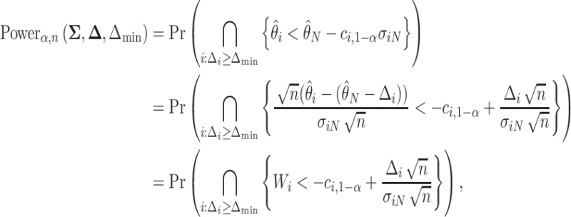
Theoretically, the bound obtained using (3.3) may be conservative, but it is often beneficial to be conservative when conducting sample size calculations because of unpredictable circumstances such as loss to follow up, patient dropout, and/or highly skewed responses. Since the normal distribution is a location-scale family, the power only depends on the vector of mean differences and not on . Henceforth, we write for the RHS of (3.3). It follows that

(3.4)

where and , and is the number of indices . Note that and do not depend on the sample size since does not depend on . If the effect sizes which are standardized by the standard deviation of the difference are specified instead of , then may be replaced by . Note that is not the same as Cohen’s d which is standardized by the pooled standard deviation rather than the standard deviation of the difference. It follows that the power may be computed by simulating normal random variables and substituting the probability in (3.4) with the empirical mean of the indicator variable as is shown in Algorithm 1.

Recall the main point of this article is to assist investigators in choosing the sample size for a SMART. To this end, we will derive a method for finding the minimum such that . We proceed by rewriting the RHS of (3.3):

(3.5)

where , , is the number of indices , and is the equicoordinate quantile for the probability in (3.5). It follows from (3.5) that . Here, we write the quantile with an asterisk to distinguish it from the quantile which controls the type I error rate . The constant may be computed using Monte Carlo simulation to find the inverse of equation (3.5) after first computing the ’s as is shown in Algorithm 2. The above procedure works because the ’s do not change with , so the distribution of is constant as a function of . Our approach for computing is an extension of the sample size computation method in the appendix of Hsu (1996) to the SMART setting when is known. Algorithms 1 and 2 are implemented in an R package “smartsizer” available at the Comprehensive R Archive Network.

Algorithm 1

SMART power computation

1. Given , compute for .

2. Given and , generate for , where , is the number of Monte Carlo repetitions, and is the number of indices .

3. Compute the Monte Carlo probability for some

In the next section, we will explore the sensitivity of the power to the covariance matrix.

4. Sensitivity of power to

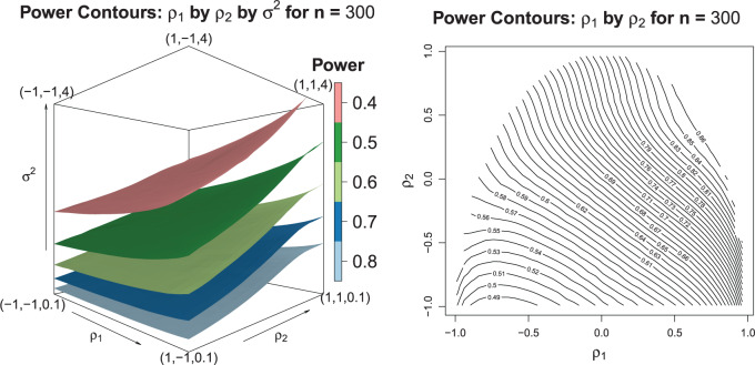
We now examine how sensitive the power is to the choice of . We will address the case in which is unknown in Section 5. For simplicity, we consider the most conservative case in which the effect sizes are all equal: for all . In Figure 2, we evaluated the power over a grid of values for using Equation (3.4) and Algorithm 1. These plots suggest the trend that higher correlations and lower variances tend to yield higher power which means that in order to obtain conservative power estimates, larger variances, and smaller correlations should be used. Furthermore, the correlation between best and non-best EDTRs appears to have a greater influence on power than the correlation between two inferior EDTRs as we see in the left-hand plot of Figure 2. We discuss this further in Section 7.

Fig. 2.

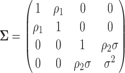The left-hand plot shows the 3D contours of the power (denoted by shade/color) as a function of where and the fourth EDTR is best. and . The right-hand plot shows power contours over the correlations where . Note that the power appears monotone with respect to and . The finger-shaped boundary is due to the feasible region of values for and such that is positive definite. The sequence of contour curves in the left-hand plot in ascending order from to corresponds to the order of the power key from 0.8 to 0.4.

It is analytically difficult to prove monotonicity for a general structure. However, it can be proven the power is a monotone non-decreasing function of the correlation and a monotone non-increasing function of the variance for an exchangeable covariance matrix. We conjecture this property is true in general for sufficiently large. To confirm that a conservative estimate of power is obtained, one may compute the power for different values of the correlation and variance and confirm the monotone trend when using a non-exchangeable covariance matrix.

Theorem 4.1

Let be exchangeable: where and . The power is an increasing function of and a decreasing function of .

Algorithm 2

SMART sample size computation

1. Given , compute for .

2. Given and , generate for where , is the number of Monte Carlo repetitions, and is the number of indices .

3. Find the equicoordinate quantile of the simulated for each .

4. The sample size is .

5. Simulation study

We have explored how the power changes in terms of a known covariance matrix. In this section, we present simulation studies for two different SMART designs in which we evaluate the assumption of a known covariance matrix. In practice, the true covariance matrix is estimated consistently by some (see Section 2.3 for more details). The designs and generating models are based on those discussed in Ertefaie and others (2015). For each SMART, we simulated 1000 datasets across a grid of sample sizes . We computed the sets of best EDTRs using the estimates and obtained using the AIPW estimation method after correctly specifying an appropriate MSM and conditional means (see Appendix A and the Tables and Figures of the supplementary material available at Biostatistics online for more details).

5.1. SMART simulation design 1

In SMART simulation design 1, the stage-2 randomization is tailored based on response to the stage-1 treatment assignment. Individuals are considered responders if and only if where is an intermediate outcome. Non-responders to the stage-1 treatment are subsequently re-randomized to one of the two intervention options while responders continue on the initial treatment assignment. We generated 1000 data sets for each sample size according to the following scheme:

1. • (a) Generate (baseline covariates)
   • (b) Generate from a Bernoulli distribution with probability (stage-1 treatment option indicator)
2. • (a) Generate and (intermediate outcomes)
   • (b) Generate from a Bernoulli distribution with probability (stage-2 treatment option indicator for non-responders)
3. Normal with unit variance and mean equal to

   

   where

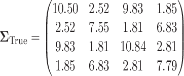
The true is . Note the first EDTR is the best. The vector of effect sizes is and the minimum detectable effect size was set to . We computed the set of best EDTRs using MCB for each data set and sample size . The empirical power was calculated as the fraction of datasets which excluded all EDTRs with true mean outcome or more away from the best EDTR (in this case EDTRs 2 and 4), for each . The true covariance matrix for this SMART was estimated using AIPW by averaging the estimated covariance matrix of 1000 simulated datasets each of 10000 individuals:

(5.6)

5.1.1. SMART simulation design 1: results

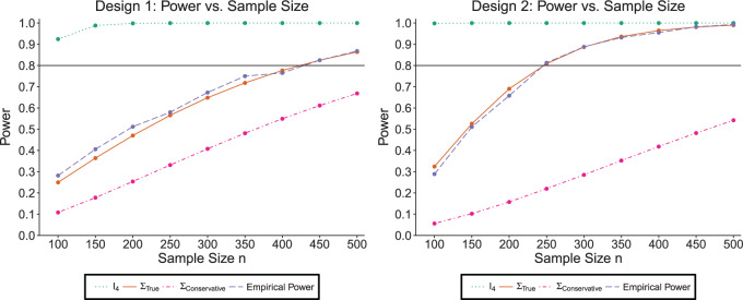
The simulation results are summarized in the plot on the left-hand side of Figure 3. The plot shows the sample size is sensitive to the choice of . Choosing will greatly underestimate the required sample size, predicting 72 individuals compared to the true 423 individuals needed to achieve power. We also looked at the power for a covariance matrix which yields a conservative estimate of power. had variances chosen to be equal to the true variances and correlations chosen to be equal to zero to achieve a lower bound on the power. The minimum sample size to achieve power for the conservative covariance matrix was .

Fig. 3.

The plots shows the power as a function of the sample size n with a horizontal line where the power is . The plot shows the power curves for , and the empirical power curve.

5.2. SMART simulation design 2

In SMART simulation design 2, stage-2 randomization depends on both prior treatment and intermediate outcomes. In particular, individuals are randomized at stage-2 if and only if they are non-responders whose stage-1 treatment option corresponded to (call this condition B). Individuals are considered responders if and only if where is an intermediate outcome. We generated 1000 data sets for each sample size according to the following scheme:

1. • (a) Generate (baseline covariates)
   • (b) Generate from a Bernoulli distribution with probability (stage-1 treatment option indicator)
2. • (a) Generate and (intermediate outcomes)
   • (b) Generate from a Multinomial distribution with probability (stage-2 treatment option indicator for individuals satisfying condition B)

3. Normal with unit variance and mean equal to where

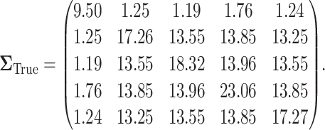
The true value is . The vector of effect sizes is and the minimum detectable effect size was set to . The set of best was computed for each data set. For each sample size, the empirical power is the fraction of data sets which exclude EDTRs 1, 2, 3, and 5. The true covariance matrix for this SMART was estimated using AIPW by averaging the estimated covariance matrices of 1000 simulated datasets each of 10000 individuals:

(5.7)

5.2.1. SMART simulation design 2: results

Our simulation results are summarized in the plot on the right-hand side of Figure 3. The power plot shows the predicted power is similar to the empirical power when assuming the correct . The anticipated sample size is 246 individuals for . Choosing yields overestimated power for each sample size, predicting 40 individuals necessary to achieve 80% power. Conversely, choosing a conservative covariance matrix underestimates the power. The is a diagonal matrix with variances set to the true variances and the correlation set to . The sample size for the conservative covariance matrix is to achieve 80% power. The loss of power when assuming the conservative covariance matrix compared with the true covariance is due to there being a high correlation between EDTR outcomes.

6. Illustration: EXTEND retrospective power calculation

In this section, we examine how much power there was to distinguish between EDTRs away from the best in the EXTEND trial. Please see Section 2.1 for more details about EXTEND and Figure 1 for a diagram depicting the trial. The true sample size was 250. The outcome of interest was the Penn Alcohol Craving Scale (PACS) and lower PACS were considered better outcomes. The covariance matrix and the vector of EDTR outcomes were estimated using both IPW and AIPW. See Table 1 for the mean EDTR outcome estimates. The covariance matrices are:

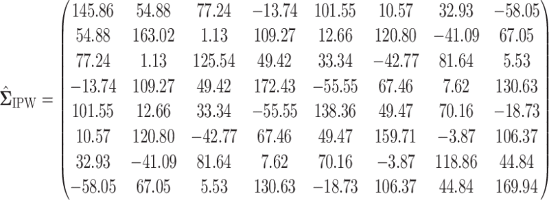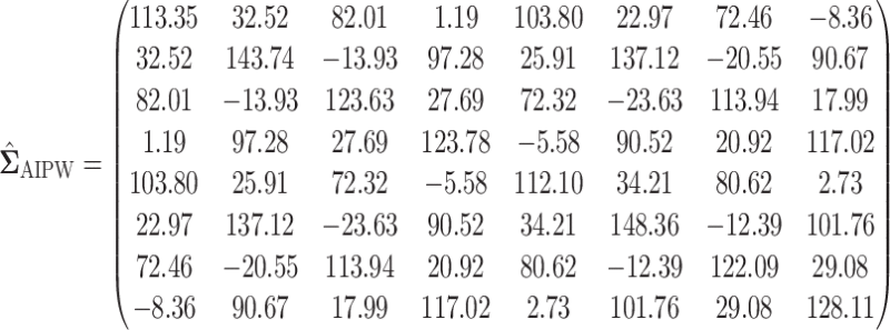Table 1.

Extend trial: EDTR outcome estimates and standard errors

IPW	Estimate	7.56	9.53	8.05	10.02	7.71	9.68	8.19	10.17
	SD	0.76	0.81	0.71	0.83	0.74	0.80	0.69	0.82
AIPW	Estimate	7.65	9.44	7.83	9.62	8.06	9.85	8.24	10.03
	SD	0.67	0.76	0.70	0.70	0.67	0.77	0.70	0.72

The EDTR outcome vectors and are summarized in Table 1. The vector of effect sizes for IPW is and for AIPW is . The set of best when performing estimation using AIPW excluded EDTRs 6 and 8. The set of best when using IPW failed to exclude any of the inferior EDTRs. In order to evaluate the power there was to exclude EDTRs 6 and 8, we set the minimum detectable effect size to .

At an level of , the power to exclude all EDTRs inferior to the best by or more was for IPW and for AIPW. AIPW yields greater power than IPW because AIPW yields smaller standard errors compared with IPW (Ertefaie and others, 2015). Our method estimates that a total of individuals would need to be enrolled to achieve a power of using IPW and a total of individuals would need to be enrolled when using AIPW.

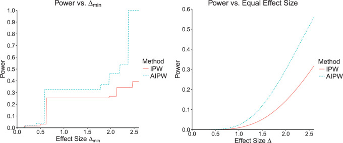
In the left-hand plot of Figure 4, we computed the power over a grid of values to see how the power changes as a function of effect size. In the right-hand side of Figure 4, we show how the power changes as a function of a uniform effect size. Specifically, we assume EDTR 1 is the best and set the effect sizes of EDTRs 2, 3,..., 8 to be equal. We then vary this uniform effect size. In this case, we ignore the actual effect sizes of the true EDTR estimates . We see the trend that AIPW yields greater power when compared with IPW.

Fig. 4.

The left-hand plot shows the power as a function of in the EXTEND trial when performing estimation with IPW and AIPW, respectively. The right-hand side of the plot shows the power as a function of the uniform effect size in the EXTEND trial when performing estimation with IPW and AIPW, respectively.

7. Guidelines for choosing the covariance matrix

We saw in Sections 4 and 5 that the power is sensitive to . However, the dependence of power on the covariance matrix is not unique to MCB. We argue this is a necessary feature of power analysis in SMART designs because it entails comparisons of correlated EDTR outcomes. We demonstrate the sensitivity of the power to the covariance matrix when sizing a SMART to detect differences in pairwise comparisons in Appendix B of the supplementary material available at Biostatistics online.

We focus on how to choose the covariance when the variances can be estimated (or an upper-bound given). We consider the situation in which the correlations are unknown in the absence of pilot SMART data and the situation in which pilot SMART data are available to estimate the correlations. In the absence of information about the correlation between EDTR outcomes, it is reasonable to assume all correlations are equal. Figure 2 illustrates that the correlation between the best EDTR and the non-best EDTR outcomes has a greater impact on power than the correlation between two non-best EDTR outcomes. Therefore, the correlation between the best EDTR and second best EDTR is important while the other correlations do not have as great an impact on the power, so we may make the working assumption that the correlations are equal. For example, the conservative covariance matrices in the simulation studies have equal correlations. Theorem 4.1 shows that the power for an exchangeable matrix is a monotone increasing function of the common correlation and a decreasing function of the variances. A similar monotone trend can be seen in Figure 2 for non-exchangeable covariance matrices. Specifically, larger variances and smaller correlations are more conservative. This is rather intuitive as if there is less variation, then it will be easier to distinguish between EDTRs.

When only an upper bound can be obtained for the variance of EDTR outcomes, one may assume a conservative exchangeable covariance matrix in which the diagonal elements are all equal to the upper bound on the variance and the correlation is set to the smallest plausible value. Information about the variances of outcomes for each EDTR may be obtained from prior non-SMART studies that provide the variation in outcomes for the treatments embedded in each EDTR. In this case, one may assume a matrix in which the diagonal elements equal the known variances and the correlation is set to the smallest plausible value. If a negative correlation between EDTR outcomes is implausible, a diagonal matrix may be chosen to obtain a conservative power estimate. For a covariance matrix in which the correlations are equal, the minimum negative correlation is bounded below by for the covariance matrix to be positive definite (Tong, 2012).

As an alternative to sizing SMARTs based off a conservative covariance matrix, we propose conducting a pilot SMART to estimate the correlations in in order to fine-tune power calculations. In addition to assisting in sample size calculations, pilot SMARTs are able to answer questions about the feasibility of the investigators to carry out the SMART and acceptability of the treatments by patients (Almirall and others, 2012; Gunlicks-Stoessel and others, 2016; Kim and others, 2016). If estimates of the variances of each EDTR outcome are known (by choosing the largest plausible values based off knowledge of the variance of response to treatments embedded in the EDTRs), the pilot SMART may be used to estimate the correlations by first estimating the full covariance matrix using AIPW and then transforming to a correlation matrix. The covariance matrix with given variances may then be obtained by left and right multiplying the correlation matrix by the square root of the diagonal matrix whose elements consist of the variances of EDTR outcomes. We propose the following algorithm: (i) conduct a pilot SMART; (ii) bootstrap times to obtain estimates of the covariance matrix using an estimation procedure such as AIPW; (iii) transform the covariance matrix estimates to correlation matrices and then use the variances of EDTR outcomes obtained from prior study data to transform back to covariance matrices; (iv) compute the sample size for each bootstrapped covariance matrix and choose the maximum sample size (or 97.5th percentile, for example). When planning the pilot SMART, it is necessary to choose the pilot SMART sample size sufficiently large so that there are patients in each EDTR in order for the covariance to be estimated. It is the subject of future work to develop methods for sizing pilot SMARTs to estimate the unknown covariance matrix to a specified accuracy. For now, we refer readers to Kim and others (2016) and Almirall and others (2012) for sizing a pilot SMART. In Appendix B of the supplementary materials available at Biostatistics online, we demonstrate the above algorithm for two simulated pilot SMARTs with individuals.

8. Final comments

If practitioners size a SMART using MCB, the study may be underpowered for conducting all pairwise comparisons since MCB yields greater power compared with approaches which entail a greater number of comparisons. Such confidence intervals obtained by all pairwise comparisons might not be sufficiently narrow. An important point is that MCB does not provide a p-value, so practitioners may wish to apply a method such as the global test for equality of EDTR outcomes (Ogbagaber and others, 2016). Sizing a SMART based off our method may overpower such an approach.

9. Discussion

One important goal of SMARTs is determination of an optimal EDTR. It is hence crucial to enroll a sufficient sample size to be able to detect the best EDTR and exclude EDTRs inferior to the best one by a clinically meaningful quantity. We introduced a novel method for carrying out power analyses for SMART designs which leverages multiple comparison with the best and Monte Carlo simulation. We saw the power is sensitive to the covariance matrix and have provided guidelines for choosing it. We illustrated our method on the EXTEND SMART to see how much power there was to exclude inferior EDTRs from the set of best and the necessary sample size to achieve power.

Other work has focused on estimating the optimal DTR (not embedded DTR) based on tailoring variables not embedded in the SMART. Such methods include Q-learning (Watkins, 1989; Chakraborty and Moodie, 2013; Ertefaie and others, 2016). These analyses are exploratory in nature and are typically not the primary goal of SMARTs. Future work will involve developing methods for sizing a SMART for such exploratory aims (Laber and others, 2016; Kidwell and others, 2018).

Software

The R package smartsizer implementing Algorithms 1 and 2 is available to download at the Comprehensive R Archive Network (https://cran.r-project.org/web/packages/smartsizer/). The R code used in this manuscript is also available to download at https://github.com/wilart/SMART-Sizer-Paper.

Funding

The NIAAA (R01 AA019092, R01 AA014851, RC1 AA019092, and P01 AA016821) (in part) and also R01 DA039901 (NIH/NIDA) and K24 DA029062 (NIDA, national institute on drug abuse). The project described in this publication was partially supported by the University of Rochester CTSA award number UL1 TR002001 from the National Center for Advancing Translational Sciences of the National Institutes of Health. The content is solely the responsibility of the authors and does not necessarily represent the official views of the National Institutes of Health.

References

- Almirall, D., Compton, S. N., Gunlicks-Stoessel, M., Duan, N. and Murphy, S. A. (2012). Designing a pilot sequential multiple assignment randomized trial for developing an adaptive treatment strategy. Statistics in Medicine 31, 1887–1902. [DOI] [PMC free article] [PubMed] [Google Scholar]
- Chakraborty, B. (2011). Dynamic treatment regimes for managing chronic health conditions: a statistical perspective. American Journal of Public Health 101, 40–45. [DOI] [PMC free article] [PubMed] [Google Scholar]
- Chakraborty, B. and Moodie, E. E. (2013). Statistical Methods for Dynamic Treatment Regimes. New York: Springer. [Google Scholar]
- Chakraborty, B. and Murphy, S. A. (2014). Dynamic treatment regimes. Annual Review of Statistics and its Application 1, 447–464. [DOI] [PMC free article] [PubMed] [Google Scholar]
- Crivello, A. I., Levy, J. A. and Murphy, S. A. (2007a). Evaluation of sample size formulae for developing adaptive treatment strategies using a smart design. Technical Report No. 07-81 University Park, PA: The Pennsylvania State University, The Methodology Center. [Google Scholar]
- Crivello, A. I., Levy, J. A. and Murphy, S. A. (2007b). Statistical methodology for a smart design in the development of adaptive treatment strategies. Technical Report No. 07-82. University Park, PA: The Pennsylvania State University, The Methodology Center. [Google Scholar]
- Ertefaie, A., Shortreed, S. and Chakraborty, B. (2016). Q-learning residual analysis: application to the effectiveness of sequences of antipsychotic medications for patients with schizophrenia. Statistics in Medicine 35, 2221–2234. [DOI] [PMC free article] [PubMed] [Google Scholar]
- Ertefaie, A., Wu, T., Lynch, K. G. and Nahum-Shani, I. (2015). Identifying a set that contains the best dynamic treatment regimes. Biostatistics 17, 135–148. [DOI] [PMC free article] [PubMed] [Google Scholar]
- Gunlicks-Stoessel, M., Mufson, L., Westervelt, A., Almirall, D. and Murphy, S. (2016). A pilot smart for developing an adaptive treatment strategy for adolescent depression. Journal of Clinical Child & Adolescent Psychology 45, 480–494. [DOI] [PMC free article] [PubMed] [Google Scholar]
- Hsu, J. C. (1981). Simultaneous confidence intervals for all distances from the “best”. The Annals of Statistics 9, 1026–1034. [Google Scholar]
- Hsu, J. C. (1984). Constrained simultaneous confidence intervals for multiple comparisons with the best. Annals of Statistics 12, 1136–1144. [Google Scholar]
- Hsu, J. C. (1996). Multiple Comparisons: Theory and Methods. London: CRC Press. [Google Scholar]
- Kidwell, K. M., Seewald, N. J., Tran, Q., Kasari, C. and Almirall, D. (2018). Design and analysis considerations for comparing dynamic treatment regimens with binary outcomes from sequential multiple assignment randomized trials. Journal of Applied Statistics 45, 1628–1651. [DOI] [PMC free article] [PubMed] [Google Scholar]
- Kim, H., Ionides, E. and Almirall, D. (2016). A sample size calculator for smart pilot studies. SIAM Undergraduate Research Online. DOI: 10.1137/15S014058. [DOI] [PMC free article] [PubMed] [Google Scholar]
- Laber, E. B., Lizotte, D. J., Qian, M., Pelham, W. E. and Murphy, S. A. (2014). Dynamic treatment regimes: technical challenges and applications. Electronic Journal of Statistics 8, 1225–1272. [DOI] [PMC free article] [PubMed] [Google Scholar]
- Laber, E. B., Zhao, Y., Regh, T., Davidian, M., Tsiatis, A., Stanford, J. B., Zeng, D., Song, R. and Kosorok, M. R. (2016). Using pilot data to size a two-arm randomized trial to find a nearly optimal personalized treatment strategy. Statistics in Medicine 35, 1245–1256. [DOI] [PMC free article] [PubMed] [Google Scholar]
- Lavori, P. W., Dawson, R. and Rush, A. J. (2000). Flexible treatment strategies in chronic disease: clinical and research implications. Biological Psychiatry 48, 605–614. [DOI] [PubMed] [Google Scholar]
- Lei, H., Nahum-Shani, I., Lynch, K. G., Oslin, D. and Murphy, S. A. (2012). A SMART design for building individualized treatment sequences. Annual Review of Clinical Psychology 8, 21–48. [DOI] [PMC free article] [PubMed] [Google Scholar]
- Murphy, S. A. (2003). Optimal dynamic treatment regimes. Journal of the Royal Statistical Society: Series B (Statistical Methodology) 65, 331–355. [Google Scholar]
- Murphy, S. A. (2005). An experimental design for the development of adaptive treatment strategies. Statistics in Medicine 24, 1455–1481. [DOI] [PubMed] [Google Scholar]
- Murphy, S. A., van der Laan, M. J., Robins, J. M.. and Conduct Problems Prevention Research Group (2001). Marginal mean models for dynamic regimes. Journal of the American Statistical Association 96, 1410–1423. [DOI] [PMC free article] [PubMed] [Google Scholar]
- Nahum-Shani, I., Ertefaie, A., Lu, X., Lynch, K. G., McKay, J. R., Oslin, D. W. and Almirall, D. (2017). A smart data analysis method for constructing adaptive treatment strategies for substance use disorders. Addiction 112, 901–909. [DOI] [PMC free article] [PubMed] [Google Scholar]
- Nahum-Shani, I., Qian, M., Almirall, D., Pelham, W. E., Gnagy, B., Fabiano, G. A., Waxmonsky, J. G., Yu, J. and Murphy, S. A. (2012). Experimental design and primary data analysis methods for comparing adaptive interventions. Psychological Methods 17, 457–477. [DOI] [PMC free article] [PubMed] [Google Scholar]
- Ogbagaber, S. B., Karp, J. and Wahed, A. S. (2016). Design of sequentially randomized trials for testing adaptive treatment strategies. Statistics in Medicine 35, 840–858. [DOI] [PMC free article] [PubMed] [Google Scholar]
- Robins, J. M. (2004). Optimal structural nested models for optimal sequential decisions. In: Proceedings of the Second Seattle Symposium in Biostatistics. New York, NY: Springer, pp. 189–326. [Google Scholar]
- Tong, Y. L. (2012). The Multivariate Normal Distribution. Springer Series in Statistics. New York: Springer. [Google Scholar]
- Watkins, C. J. C. H. (1989). Learning from delayed rewards [Ph.D. Thesis]. Cambridge: King’s College. [Google Scholar]
Associated Data
This section collects any data citations, data availability statements, or supplementary materials included in this article.