HIV and shifting epicenters for COVID-19, an alert for some countries

Abstract

Were southern hemisphere countries right to undertake national lockdown during their summer time? Were they right to blindly follow the self-isolation wave that hit European countries in full winter? As a southern hemisphere country like South Africa stands now as the most COVID-19 and HIV affected country in Africa, we use in this paper, recent COVID-19 data to provide a statistical and comparative analysis that may alert southern hemisphere countries entering the winter season. After that, we use a generalized simple mathematical model of HIV-COVID-19 together with graphs, curves and tables to compare the pandemic situation in countries that were once the epicenter of the disease, such as China, Italy, Spain, United Kingdom (UK) and United States of America (USA). We perform stability and bifurcation analysis and show that the model contains a forward and a backward bifurcation under certain conditions. We also study different scenarios of stability/unstability equilibria for the model. The fractional (generalized) COVID-19 model is solved numerically and a predicted prevalence for the COVID-19 is provided. Recall that Brazil and South Africa share number of similar social features like Favellas (Brazil) and Townships (South Africa) with issues like promiscuity, poverty, and where social distanciation is almost impossible to observe. We can now ask the following question: Knowing its HIV situation, is South Africa the next epicenter in weeks to come when winter conditions, proven to be favorable to the spread of the new coronavirus are comfily installed?

1. Introduction

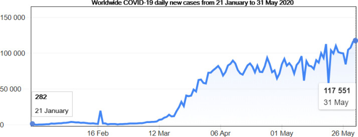
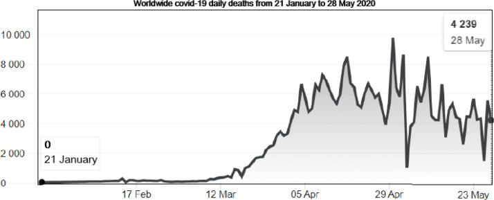
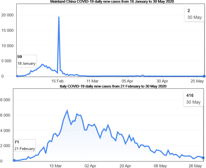
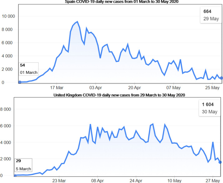
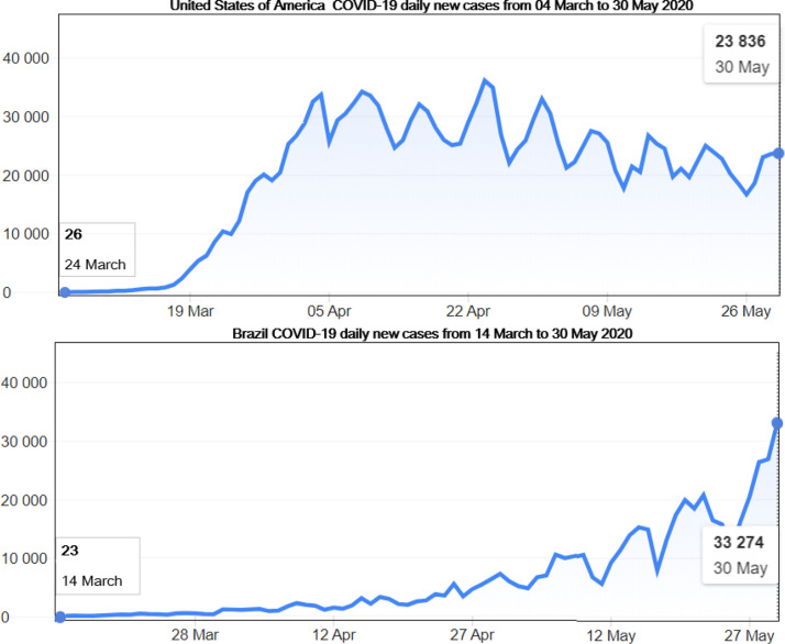
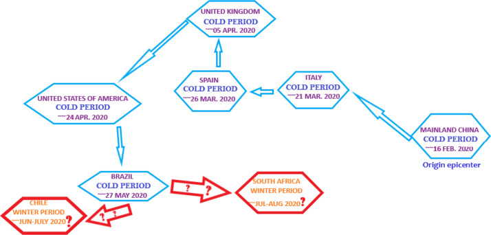
It is in December 2019 that a new pneumonia, today known as coronavirus disease 2019 or shorlty COVID-19, locally started off in the Chinese city of Wuhan. As of 30 May 2020, the world recorded almost 5.96 million cases of COVID-19 reported worldwide in about 188 countries, nations and territories. Among those reported cases, almost 366,000 people have succumbed to the disease (Figs. 1 and 8) but fortunately, almost 2.52 million people have recovered. It is only on 11 March 2020 that the World Health Organization (WHO) declared the COVID-19 a pandemic. Maybe this unprecedented situation, since the 1918 Spanish flu pandemic [1], would have been different if the alert call from Li Wenliang [2] was taken into consideration on time by Chinese authorities. Hence, the worldwide epicenter of the disease has since hit several countries, from China to USA via Italy, Spain and UK ( Fig. 2, Fig. 3, Fig. 4 and 6). It has now moved to the southern hemisphere country of Brazil with the winter season (Fig. 4).

Fig. 1.

Illustration of Worldwide COVID-19 daily new cases from 21 January to 31 May 2020 according to the WHO Coronavirus disease (COVID-2019) situation reports [4]. We note that the number of infections keep rising meaning that the pandemic is far from being over.

Fig. 8.

Illustration of worldwide COVID-19 daily deaths from 21 January to 28 May 2020 according to the WHO Coronavirus disease (COVID-2019) situation reports [4]. We note that the number of deaths has peaked some times around 29 April 2020 but remain significant in around the world, with exactly 4239 reported on 28 May.

Fig. 2.

Illustration of two former epicenters, China and Italy COVID-19 daily new cases from 21 January to 30 May 2020 according to the WHO Coronavirus disease (COVID-2019) situation reports [4]. We note that the number of infections kept rising until the peak was reached before a decrease. The rise in China was quickly contained, around 16 Feb., before Italy took over the epicenter status until around 21 Mar. 2020.

Fig. 3.

Illustration of two former epicenters, Spain and UK COVID-19 daily new cases from the start of the pandemic (01 march for Spain and 29 March for UK) until 30 May 2020 according to the WHO Coronavirus disease (COVID-2019) situation reports [4]. We note that the number of infections kept rising until the peak was reached before a decrease. The rise in Spain was contained around 1 April 2020, before UK took over the epicenter status around 05 April 2020.

Fig. 4.

Illustration of one former epicenter, USA and the actual epicenter Brazil showing their COVID-19 daily new cases from the start of the pandemic (14 March for Brazil and 24 March for USA) until 30 May 2020 according to the WHO Coronavirus disease (COVID-2019) situation reports [4]. The USA quickly became the new epicenter of the disease around 24 April before starting seing a slight relief around. Though the number of new infections is still high i USA, Brazil has the new epicenter around 27 May 2020.

Fig. 6.

Worldwide shifting epicenters from China to Brazil and the approximative time they were epicenters. Is Chile or South Africa the next one as they enter the winter season?.

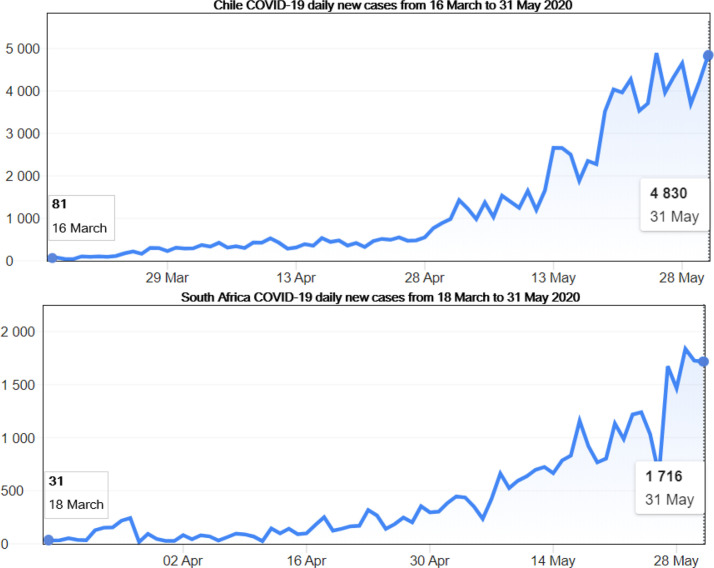
Highly contagious, COVID-19 is caused by severe acute respiratory syndrome coronavirus 2 (SARS-CoV-2) and has been proven to spread easily when cold winter conditions are met. In fact, some research made recently [3] have shown that the SARS-CoV-2 can easily spread in communities that live in places where the temperature is relatively low, around 5 to 11 degrees Celsius, all associated with low specific, of around 3 to 6 g/kg and absolute humidity of around 4 to 7 g/m ³. As southern hemisphere moves to the winter season, there are worries to feel for two particular countries whose the number of deaths keeps rising: Chile and South Africa (Figs. 5 and 7 ). More worries for South Africa as the country stands not only as the current most COVID-19 affected country in Africa but also the most HIV affected country. Moreover, the alarming situation in Brazil should be a huge concern for South Africa as both countries face similar precarious social issues as shown in Table 1 . Recent statistics [4], [5] show that COVID-19 mostly kills people with pre-existing diseases such as diabetes, high blood pressure, tuberculosis and also HIV. Hence, this motivated us to study in this paper, a combined HIV-COVID-19 model is order to start another alert call for those concerned countries at risk.

Fig. 5.

Illustration of potential next epicenter: Chile and South Africa COVID-19 daily new cases from the start of the pandemic (16 March for Chile and 18 March for South Africa) until 30 May 2020 according to the WHO Coronavirus disease (COVID-2019) situation reports [4]. It shows that the number of new infections keeps rising in both countries.

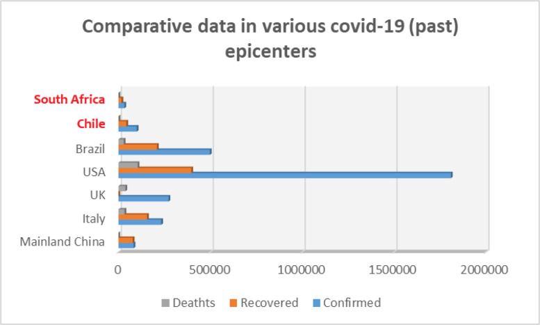
Fig. 7.

Comparative illustration of COVID-19 victims as from 1 June 2020 in all past and current epicenters. We note the global numbers are still relatively low in Chile and South Africa and up-front alerts need to be heard now before it is too late.

Table 1.

Comparison of some factors [3], [6], [7] favorable to the spread of Covi-19 in Brazil (current epicenter) and South Africa (the potential next).

	FAVELLAS	TOWNSHIPS
Country	Brazil	South Africa
Approximative population	11 million (6%)	14.7 million (25%)
(% of the total population)
Residents	Mainly African descents	Mainly Africans
Characteristics	Poverty, sanitation, water,	Poverty, infrastructure
	garbage collection	problems,water supply problem
	promiscuity	densely populated
COVID-19 state	Most affected in Latin America	Most affected in Africa
Feature	The country’s president	The country’s president
	chose not to go for a	chose to easy the lockdown
	hard lockdown despite an	despite an increasing
	increasing number of deaths	number of deaths

2. A simple COVID-19 model combined to HIV

2.1. A simple HIV-COVID-19 model formulation and assumptions

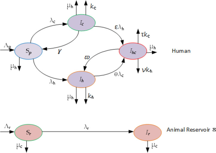
As commonly done in mathematical epidemiology for other type of diseases [8], [9], [10], [11], [12], [13], [14], [15], we start by formulating the model and clarifying the assumptions that will be used throughout. In this section, a simple system modeling the temporal dynamics of the Corona virus (2019-nCov) combined to HIV within human population is described. As we don’t have yet all the answers on the real dynamics and spread of the new 2019-nCov, we focus on people who are already COVID-19 infectious (symptomatic or asymptomatic individuals). We assume the people population N_p to be constant and divide it into four different compartments according to their status with respect to the diseases. Hence, at the t, we denote by $S_p=S_p\left(t\right)$ the fraction of the people population that are susceptible, by $I_c=I_c\left(t\right)$ the fraction of the people population that is COVID-19 only infectious, by $I_h=I_h\left(t\right)$ the fraction of the people population that is HIV only infectious, by $I_{hc}=I_{hc}\left(t\right)$ the fraction of the people population that is dually infectious with HIV and COVID-19. We assume that the COVID-19 infection process originates from a reservoir or a source of infection (called Ξ) with animals (pangolin or bats, etc) with a total population of $N_r=N_r\left(t\right)$ that can be divided into two different compartments: The susceptible to COVID-19 ($S_r=S_r\left(t\right)$) and COVID-19 infectious ($I_r=I_r\left(t\right)$). We assume that individuals in the susceptible compartment are recruited into the people population at a rate Λ_p which is constant. Infections with COVID-19 of those individuals happen at a rate of λ_c due to sufficient contact with infected animals in Ξ, and they then move to the compartment of COVID-19 infectious individuals, I_c. Moreover, infections with HIV happen at a rate of λ_h due to sufficient contact with infected individuals and therefore, susceptible individuals move to the compartment of HIV infectious individuals, I_h. People who are infected with COVID-19 only either recover thanks to their own immunity and are moved, at a rate of γ, into the compartment of susceptible individuals or are infected with HIV due to sufficient contact with infected individuals, at the fraction rate of ελ_h, (with ε ∈ (0, 1]. Recall [16] that ε is taken as such because we expect an eventual drop of sexual intercourse (principal known cause of HIV transmission) of people who are infected with COVID-19 due to the disease. They then move into the compartment I_hc of dually infectious with HIV and COVID-19. The disease COVID-19 kills people at the rate of κ_c. People who are infected with HIV only either die due to the disease or get the infection with Corona virus, at the rate of θλ_h, due to sufficient contact with infected source. They then move into the compartment I_hc of dually infectious with HIV and COVID-19. Here we take θ > 1 since people infected with HIV have a lower immune system and therefore, are highly susceptible to catch COVID-19. Individuals with both HIV and COVID-19 can recover from COVID-19 thanks to own immunity and are moved, at a rate of ϖ into the compartment of individuals infected with HIV only or die from COVID-19 at the rate of τκ_c. Here we take τ > 1 because of the high probability of mortality within the people in I_hc, with both HIV and COVID-19 compared to individuals infected with COVID-19 only. Furthermore, individuals with both HIV and COVID-19 can also die HIV at a rate of νκ_h. Here we take ν ≥ 1 because of the high probability of mortality within the people in I_hc, with both HIV and COVID-19 compared to individuals infected with HIV only. We denote by μ_h the rate at which death due natural causes occurs. We assume that susceptible animals in Ξ, are recruited into the population N_r at a rate of Λ_r which is constant. We assume that those animals can die the rate of μ_c or can become infected with COVID-19 at a rate of λ_r due to sufficient contact with infected animals and then move to the compartment of COVID-19 infectious I_r. Based on the above setting, the dynamics of the system is given by the transfer diagram as depicted in Fig. 10 and expressed by the following differential equations:

$$\{\begin{array}{c}{\displaystyle \frac{S_p}{dt}={\Lambda }_p+\gamma I_c-({\lambda }_c+{\lambda }_h+{\mu }_h)S_p,}\hfill \\ {\displaystyle \frac{I_c}{dt}={\lambda }_c{S}_p-(\epsilon {\lambda }_h+{\mu }_h+{\kappa }_c+\gamma )I_c,}\hfill \\ {\displaystyle \frac{I_h}{dt}={\lambda }_h{S}_p+\varpi I_{hc}-(\theta {\lambda }_c+{\mu }_h+{\kappa }_h)I_h,}\hfill \\ {\displaystyle \frac{I_{hc}}{dt}=\epsilon {\lambda }_h{I}_c+\theta {\lambda }_c{I}_h-({\mu }_h+\tau {\kappa }_c+\nu {\kappa }_h+\varpi )I_{hc},}\hfill \\ {\displaystyle \frac{S_r}{dt}={\Lambda }_r-({\mu }_c+{\lambda }_r)S_r}\hfill \\ {\displaystyle \frac{I_r}{dt}={\lambda }_r{S}_r-{\mu }_c{I}_r,}\hfill \end{array}$$ (1)

where λ_c, λ_h and λ_r are respectively the forces of infection reading as

$${\lambda }_c=\frac{{\beta }_c\sigma I_r}{N_p},$$

$${\lambda }_h=\frac{{\beta }_h(I_h+{\xi }_{hc}{I}_{hc})}{N_p},$$

$${\lambda }_r=\frac{{\beta }_r\sigma I_r}{N_r},$$

with β_h representing the HIV infection effective contact rate, ξ_hc ≥ 1 representing the regularization parameter modeling the relative infectiousness of people with both HIV and COVID-19 (I_hc) compared to individuals infected with HIV only (I_h). For the new corona virus (2019-nCov), σ is the per capita vector-to-host contact rate of the animals in the reservoir. β_c is the parameter accounting for the people transmission probability per vector-to-host contact while β_r accounts for the same probability but for animals.

Fig. 10.

Flowdiagram of the HIV-COVID-19 transmission between people and in the reservoir.

3. Sub-model’s analysis: Well-posedness, feasibility region and stability

In this section we start by analyzing the two sub-models (HIV only and COVID-19 only) contained in the model (1).

4. Sub-model: HIV only

We establish the HIV only sub-model from model (1) by putting $I_c=0,I_{hc}=0,S_r=0,I_r=0$ which yields

$$\{\begin{array}{c}{\displaystyle \frac{S_p}{dt}={\Lambda }_p-({\lambda }_h+{\mu }_h)S_p,}\hfill \\ {\displaystyle \frac{I_h}{dt}={\lambda }_h{S}_p-({\mu }_h+{\kappa }_h)I_h,}\hfill \end{array}$$ (2)

with the force of infection λ_h reading as

$${\lambda }_h=\frac{{\beta }_h{I}_h}{N_p},$$

where $N_p=S_p+I_h.$ In order analyze the HIV only system (2) of human population, we consider the region of biological feasibility given by.

$${\Omega }_h=\{(S_p\left(t\right),I_h\left(t\right))\in {\mathbb{R}}^2:0\le N_p=S_p+I_h\le \frac{{\Lambda }_p}{{\mu }_h}\}.$$

we have the following results

Proposition 4.1

• 1.Any solution (S_p(t), I_h(t)) of the HIV only system (2) remains non-negative for all time t > 0 if the corresponding initial condition is non-negative.
• 2.the region Ω_h is positively invariant for the HIV only system (2) when non-negative initial conditions are taken from ${\mathbb{R}}^2.$ In fact it is an attracting and absorbing compact set for the system (2) .
• 3.
  Moreover, we have

  $$\underset{t\to \infty }{\lim }{N}_p\left(t\right)\le \frac{{\Lambda }_p}{{\mu }_h}.$$

  and$N_p\left(t\right)\le \frac{{\Lambda }_p}{{\mu }_h}$for all t > 0 if $N_p\left(0\right)\le \frac{{\Lambda }_p}{{\mu }_h}.$

Proof

The sum of both equations of (2) gives

$$\begin{array}{ccc}\hfill \frac{d{N}_p\left(t\right)}{dt}& =& \frac{d{S}_p\left(t\right)}{dt}+\frac{d{I}_h\left(t\right)}{dt}\hfill \\ & =& {\Lambda }_p-{\mu }_h(S_p\left(t\right)+I_h\left(t\right))-{\kappa }_h{I}_h\hfill \\ & \le & {\Lambda }_p-{\mu }_h{N}_p\left(t\right)\hfill \end{array}$$ (3)

proceeding with standard comparison and integration give

$$\begin{array}{ccc}\hfill N_p\left(t\right)& \le & N_p\left(0\right){\text{e}}^{-{\mu }_{h}t}-\frac{{\Lambda }_p}{{\mu }_h}{\text{e}}^{-{\mu }_{h}t}\hfill \\ & \le & (N_h\left(0\right)-\frac{{\Lambda }_p}{{\mu }_h}){\text{e}}^{-{\mu }_{h}t}+\frac{{\Lambda }_p}{{\mu }_h}\hfill \end{array}$$

Hence we have $N_p\left(t\right)\le \frac{{\Lambda }_p}{{\mu }_h}\text{for}\text{all}\text{time}t\ge 0,$ if $N_p\left(0\right)-\frac{{\Lambda }_p}{{\mu }_h}\le 0$ (or $N_p\left(0\right)\le \frac{{\Lambda }_p}{{\mu }_h}$). This conclusion also shows the attractiveness and absorbing results for Ω. □

The HIV only system (2) can therefore be treated as dynamical system in Ω in which it is well-posed.

4.1. The basic reproduction number ${\mathcal{R}}_h$

The disease-free equilibrium (or the DFE) of the HIV only system (2) reads as

$$E^0=(S_p^0,I_h^0)\text{with}(S_p^0=\frac{{\Lambda }_p}{{\mu }_h},I_h^0=0).$$

Exploiting the next generation operator $F{V}^{-1}$ as detailed in [17] leads to the HIV only system (2) written into the matrix form $\dot{X}=\mathcal{F}\left(X\right)-\mathcal{V}\left(X\right)$ where the matrices $\mathcal{F}$ and $\mathcal{V}$ are respectively given by

$$\mathcal{F}\left(X\right)=\left(\begin{array}{c}0\\ {\lambda }_h\left(t\right)S_p\left(t\right)\end{array}\right)$$

and

$$\mathcal{V}\left(X\right)=\left(\begin{array}{c}-{\Lambda }_p+{\lambda }_h\left(t\right)S_p\left(t\right)+{\mu }_h{S}_p\left(t\right)\\ {\mu }_h{I}_h\left(t\right)+{\kappa }_h{I}_h\left(t\right)\end{array}\right)$$

Evaluated at the DFE E ⁰, the Jacobian of those matrices yields

$$F=\left[\frac{\partial {\mathcal{F}}_i}{\partial x_j}\left(E^0\right)\right]=\left({\beta }_h\right)$$

and

$$V=\left[\frac{\partial {\mathcal{V}}_i}{\partial x_j}\left(E^0\right)\right]=({\mu }_h+{\kappa }_h).$$

Hence the basic reproduction number ${\mathcal{R}}_h$ is the spectral radius

$${\mathcal{R}}_h=\rho \left(F{V}^{-1}\right)=\frac{{\beta }_h}{{\mu }_h+{\kappa }_h}.$$

4.2. Stability of the DFE E⁰

Using the linearization of the HIV only system (2) around the DFE E ⁰ we obtain the Jacobian matrix reading as

$${\mathcal{J}|}_{E^0}=\left(\begin{array}{cc}-{\mu }_h& -{\beta }_h\\ 0& {\beta }_h-{\mu }_h-{\kappa }_h\end{array}\right).$$ (4)

We easily obtain the eigenvalues ${\mathcal{J}|}_{E^0}$ that reads as: ${\lambda }_1=-{\mu }_h$ which is negative and ${\lambda }_2={\beta }_h-{\mu }_h-{\kappa }_h.$ In terms of ${\mathcal{R}}_h,$ we have ${\lambda }_2=({\mu }_h+{\kappa }_h)({\mathcal{R}}_h-1)$. Hence ${\lambda }_2<0⟺{\mathcal{R}}_h<1.$ Thus, we have proven the following result

Proposition 4.2

The DFE E⁰of the model(2)is locally-asymptotically stable if${\mathcal{R}}_h<1,$and unstable if${\mathcal{R}}_h>1.$

For the establishment of global asymptotical stability of the DFE E ⁰, we can use the method of Lyapunov-LaSalle by considering a Lyapunov function $L(S_p,I_h)=({\mu }_h+{\kappa }_h)I_h.$ Then its time-derivative along a solution (S_p(t), I_h(t)) reads as

$$\begin{array}{ccc}\hfill \frac{dL}{dt}& =& ({\mu }_h+{\kappa }_h)\frac{d{I}_h}{dt}\hfill \\ & =& ({\mu }_h+{\kappa }_h)({\lambda }_h{S}_p-({\mu }_h+{\kappa }_h)I_h)\hfill \\ & =& (\frac{{\beta }_h{S}_h}{N_p({\mu }_h+{\kappa }_h)}-1)\frac{{\lambda }_h({\mu }_h^2+{\kappa }_h^2+2{\mu }_h{\kappa }_h)N_p}{{\beta }_h}\hfill \\ & \le & (\frac{{\beta }_h}{({\mu }_h+{\kappa }_h)}-1)\frac{{\lambda }_h({\mu }_h^2+{\kappa }_h^2+2{\mu }_h{\kappa }_h)N_p}{{\beta }_h}\hfill \\ & \le & ({\mathcal{R}}_h-1)\frac{{\lambda }_h({\mu }_h^2+{\kappa }_h^2+2{\mu }_h{\kappa }_h)N_p}{{\beta }_h},\hfill \end{array}$$

where we have used the fact that $\frac{S_h}{N_p}\le 1.$ Hence, knowing that the system parameters are all non-negative, $\frac{dL}{dt}\le 0$ when ${\mathcal{R}}_h\le 1.$ Moreover, it happens that $\frac{dL}{dt}=0⟺I_h=0.$

Therefore, L is a Lyapunov function on Ω_h and LaSalle’s Invariance Principle [18] implies that all limit points of solutions to the model (2) belong to the largest compact invariance set in $\{(S_p\left(t\right),I_h\left(t\right))\in {\Omega }_h:\frac{dL}{dt}=0\}.$ In that set, $I_h=0$ and $\frac{d{S}_p}{dt}={\Lambda }_p-{\mu }_h{S}_p$ and thus $S_p⟶\frac{{\Lambda }_p}{{\mu }_h}$ as $t⟶\infty .$ Thus, Therefore, every solution (S_p(t), I_h(t)), taking its initial conditions in Ω_h, approaches the DFE $E^0=(\frac{{\Lambda }_p}{{\mu }_h},0)$ as $t⟶\infty$ when ${\mathcal{R}}_h\le 1.$ Henceforth, we have proven the following result:

Proposition 4.3

The DFE E⁰of the model(2)is globally-asymptotically stable whenever${\mathcal{R}}_h\le 1.$

4.3. Endemic equilibrium

From (2) the endemic equilibrium $E^{*}=(S_p^{*},I_h^{*})$ is obtained by solving

$$\{\begin{array}{c}0={\Lambda }_p-({\lambda }_h^{*}+{\mu }_h)S_p^{*},\hfill \\ 0={\lambda }_h^{*}{S}_p^{*}-({\mu }_h+{\kappa }_h)I_h^{*},\hfill \end{array}$$ (5)

which yields

$$S_p^{*}=\frac{{\Lambda }_p}{{\mu }_h+{\lambda }_h^{*}},I_h^{*}=\frac{{\Lambda }_p{\lambda }_h^{*}}{({\mu }_h+{\kappa }_h)({\mu }_h+{\lambda }_h^{*})}$$ (6)

with the force of infection

$${\lambda }_h^{*}=\frac{{\beta }_h{I}_h^{*}}{(S_p^{*}+I_h^{*})}.$$ (7)

Simple transformation of (6) and (7) leads to following polynomial in ${\lambda }_h^{*}:$

$${\lambda }_h^{*}({\lambda }_h^{*}+(1-{\mathcal{R}}_h)({\mu }_h+{\kappa }_h))=0.$$ (8)

Hence we have ${\lambda }_h^{*}=-(1-{\mathcal{R}}_h)({\mu }_h+{\kappa }_h)$ which has a biological meaning only if the force of infection ${\lambda }_h^{*}$ is non negative, meaning that $(1-{\mathcal{R}}_h)({\mu }_h+{\kappa }_h)<0⟺{\mathcal{R}}_h>1.$ Furthermore, in terms of ${\mathcal{R}}_h,$ (6) gives

$$S_p^{*}=\frac{{\Lambda }_p}{{\kappa }_h({\mathcal{R}}_h-1)+{\mu }_h{\mathcal{R}}_h},I_h^{*}=\frac{({\mathcal{R}}_h-1){\Lambda }_p}{{\kappa }_h({\mathcal{R}}_h-1)+{\mu }_h{\mathcal{R}}_h}.$$ (9)

We have then shown the results

Lemma 4.4

The model(2)of HIV has a unique endemic equilibrium if and only if${\mathcal{R}}_h>1.$Moreover, that unique endemic equilibrium locally asymptotically stable if${\mathcal{R}}_h>1.$

5. Sub-model: COVID-19 only

We establish the COVID-19 only sub-model from model (1) by putting $I_h=0,I_{hc}=0$ which yields

$$\{\begin{array}{c}{\displaystyle \frac{S_p}{dt}={\Lambda }_p+\gamma I_c-({\lambda }_c+{\mu }_h)S_p,}\hfill \\ {\displaystyle \frac{I_c}{dt}={\lambda }_c{S}_p-({\mu }_h+{\kappa }_c+\gamma )I_c,}\hfill \\ {\displaystyle \frac{S_r}{dt}={\Lambda }_r-({\mu }_c+{\lambda }_r)S_r}\hfill \\ {\displaystyle \frac{I_r}{dt}={\lambda }_r{S}_r-{\mu }_c{I}_r,}\hfill \end{array}$$ (10)

with the force of infection λ_c and λ_r reading respectively as

$${\lambda }_c=\frac{{\beta }_c\sigma I_r}{N_p},$$

and

$${\lambda }_r=\frac{{\beta }_r\sigma I_r}{N_r},$$

5.1. Basic reproduction number

The disease-free equilibrium (or the DFE) of the COVID-19 only system (10) reads as

$$E^0=(\frac{{\Lambda }_p}{{\mu }_h},0,\frac{{\Lambda }_r}{{\mu }_c},0)$$

Exploiting the next generation operator $F{V}^{-1}$ as detailed in [17] leads to the COVID-19 only system (10) written into the matrix form $\dot{X}=\mathcal{F}\left(X\right)-\mathcal{V}\left(X\right)$ where the matrices $\mathcal{F}$ and $\mathcal{V}$ are respectively given by

$$\mathcal{F}\left(X\right)=\left(\begin{array}{c}{\displaystyle \frac{{\beta }_c\sigma I_r\left(t\right)S_p\left(t\right)}{I_c\left(t\right)+S_p\left(t\right)}}\\ {\displaystyle \frac{{\beta }_r\sigma I_r\left(t\right)S_r\left(t\right)}{I_r\left(t\right)+S_r\left(t\right)}}\\ 0\\ 0\end{array}\right)$$

and

$$\mathcal{V}\left(X\right)=\left(\begin{array}{c}-({\mu }_h+{\kappa }_c+\gamma )I_c\left(t\right)\\ -{\mu }_c{I}_r\\ {\Lambda }_p+\gamma I_c-\left({\displaystyle {\mu }_h+\frac{{\beta }_c\sigma I_r\left(t\right)}{I_c\left(t\right)+S_p\left(t\right)}}\right)S_p\left(t\right)\\ {\Lambda }_r-\left({\displaystyle {\mu }_c+\frac{{\beta }_r\sigma I_r\left(t\right)}{I_r\left(t\right)+S_r\left(t\right)}}\right)S_r\left(t\right)\end{array}\right)$$

Evaluated at the DFE E ⁰, the Jacobian of those matrices yields

$$F=\left[\frac{\partial {\mathcal{F}}_i}{\partial x_j}\left(E^0\right)\right]=\left(\begin{array}{cc}0& {\beta }_c\sigma \\ 0& {\displaystyle {\beta }_r\sigma \frac{{\Lambda }_p^2{\mu }_c^2}{{\mu }_h^2{\Lambda }_r^2}}\end{array}\right)$$

and

$$V=\left[\frac{\partial {\mathcal{V}}_i}{\partial x_j}\left(E^0\right)\right]=\left(\begin{array}{cc}{\mu }_h+{\kappa }_c+\gamma & 0\\ 0& {\mu }_c\end{array}\right).$$

Hence the basic reproduction number ${\mathcal{R}}_c$ is the spectral radius

$${\mathcal{R}}_c=\rho \left(F{V}^{-1}\right)={\beta }_r\sigma {\left(\frac{{\Lambda }_p}{{\mu }_h}\right)}^2\frac{{\mu }_c}{{\Lambda }_r^2}.$$

Following the same approach as in Proposition 4.2, we easily show that

Proposition 5.1

The DFE$E^0=(\frac{{\Lambda }_p}{{\mu }_h},0,\frac{{\Lambda }_r}{{\mu }_c},0)$of the COVID-19 only sub-model(10)is locally-asymptotically stable if${\mathcal{R}}_c<1,$and unstable if${\mathcal{R}}_c>1.$

6. Possibility of backward bifurcation for the COVID-19 sub-model

Our aim here in this section is to look at the conditions under which there exists a backward bifurcation for the model (10). Recall that this type of bifurcation happens when a stable DFE and a stable endemic equilibrium exist together for some values of the basic reproduction number ${\mathcal{R}}_c$ less than one. Hence, we have to find conditions for which endemic equilibrium $E^{*}=(S_p^{*},I_c^{*},S_r^{*},I_r^{*}).$ We pose

$$\{\begin{array}{c}0={\Lambda }_p+\gamma I_c-({\lambda }_c+{\mu }_h)S_p,\hfill \\ 0={\lambda }_c{S}_p-({\mu }_h+{\kappa }_c+\gamma )I_c,\hfill \\ 0={\Lambda }_r-({\mu }_c+{\lambda }_r)S_r\hfill \\ 0={\lambda }_r{S}_r-{\mu }_c{I}_r,\hfill \end{array}$$

which yields

$$S_p^{*}=\frac{{\Lambda }_p({\mu }_h+{\kappa }_c+\gamma )}{{\lambda }_c^{*}({\mu }_h+{\kappa }_c)+{\mu }_h({\mu }_h+{\kappa }_c+\gamma )}$$

$$I_c^{*}=\frac{{\Lambda }_p{\lambda }_c^{*}}{{\lambda }_c^{*}({\mu }_h+{\kappa }_c)+{\mu }_h({\mu }_h+{\kappa }_c+\gamma )}$$ (11)

$$S_r^{*}=\frac{{\Lambda }_r}{{\lambda }_r^{*}+{\mu }_c}$$

$$I_r^{*}=\frac{{\Lambda }_r{\lambda }_r^{*}}{{\mu }_c({\lambda }_r^{*}+{\mu }_c)}$$

with the forces of infection

$${\lambda }_c^{*}=\frac{{\beta }_c\sigma I_r^{*}}{(S_p^{*}+I_c^{*})},{\lambda }_r^{*}=\frac{{\beta }_r\sigma I_r^{*}}{(S_r^{*}+I_r^{*})}$$ (12)

Simple transformation of (11) and (12) leads to following polynomial in ${\lambda }_c^{*}:$

$${\lambda }_c^{*}(Q_1{\left({\lambda }_c^{*}\right)}^2+Q_2{\lambda }_c^{*}+Q_3)=0.$$ (13)

where

$$Q_1={\Lambda }_p{\mu }_c({\mu }_c+{\beta }_r\sigma ),$$

$$Q_2=(T-{\mathcal{R}}_c)\frac{{\Lambda }_p{\mu }_c^2({\mu }_h+{\kappa }_c+\gamma )({\mu }_h+{\kappa }_c)}{{\mu }_h},$$

$$Q_3=(1-{\mathcal{R}}_c){\Lambda }_p{\mu }_c^2{({\mu }_h+{\kappa }_c+\gamma )}^2$$

and

$$T=\frac{(2{\mu }_c+{\beta }_r\sigma ){\mu }_h}{{\mu }_c({\mu }_h+{\kappa }_c)}$$

We have here many endemic equilibrium points (solutions ${\lambda }_c^{*}$) to

$$Q_1{\left({\lambda }_c^{*}\right)}^2+Q_2{\lambda }_c^{*}+Q_3$$ (14)

and the solution (${\lambda }_c^{*}=0$) that is related to the DEF. Let

$$\tilde{\sigma }=\frac{({\kappa }_c-{\mu }_h){\mu }_c}{{\beta }_r{\mu }_h}$$

then clearly

$$T>1⟺\sigma >\tilde{\sigma }.$$ (15)

We have the following results

Proposition 6.1

• The necessary condition for the existence of backward (subcritical) bifurcation for the model(10)is$\sigma <\tilde{\sigma }.$Furthermore, there is$0<{\tilde{\mathcal{R}}}_c<1$so that:

• - Model(10)has one and only one endemic equilibrium point if${\tilde{\mathcal{R}}}_c={\mathcal{R}}_c.$

• - Model(10)has two endemic equilibrium points if${\mathcal{R}}_c\in ({\tilde{\mathcal{R}}}_c,1).$

• - Model(10)has one endemic equilibrium point if${\mathcal{R}}_c\ge 1.$

• - Model(10)has no endemic equilibrium point if${\mathcal{R}}_c<{\tilde{\mathcal{R}}}_c.$

• The necessary condition for the existence of transcritical bifurcation for the model(10)is$\sigma \ge \tilde{\sigma }.$

Proof

To prove this, we use the equivalence relation (13)-(15) where it is obvious to see that Q ₁ > 0. Moreover, Q ₂ > 0 if $T>{\mathcal{R}}_c$ and Q ₂ < 0 if $T<{\mathcal{R}}_c.$ Also Q ₃ > 0 if ${\mathcal{R}}_c<1$ and Q ₃ < 0 if ${\mathcal{R}}_c>1.$

From (15) we have T < 1 when $\sigma <\tilde{\sigma }.$ Hence, when ${\mathcal{R}}_c\ge 1,$ we have Q ₂ ≤ 0 meaning ${\mathcal{R}}_c\ge 1>T$ and Q ₃ ≤ 0, and Eq. (14) has one and only one positive root. However, Eq. (14) has no positive root when ${\mathcal{R}}_c\le T<1$ meaning Q ₂ ≥ 0 and Q ₃ > 0.

Now in the case where $1\ge {\mathcal{R}}_c>T$ we also have Q ₂ < 0 and Q ₃ ≥ 0. If $\Delta :=F\left({\mathcal{R}}_c\right)=Q_2^2-4Q_1{Q}_3$ denotes the discriminant of (14) and a functional of ${\mathcal{R}}_c$ then

$$\begin{array}{ccc}\hfill F^{\prime }\left({\mathcal{R}}_c\right)& =& -2{(T-{\mathcal{R}}_c)}^2\frac{{\Lambda }_p{\mu }_c^2({\mu }_h+{\kappa }_c+\gamma )({\mu }_h+{\kappa }_c)}{{\mu }_h}\hfill \\ & & +4Q_1{\Lambda }_p{\mu }_c^2{({\mu }_h+{\kappa }_c+\gamma )}^2>0\hfill \end{array}$$

for ${\mathcal{R}}_c\in (T,1).$ F is strictly increasing in (T, 1) and $F\left(T\right)=-4Q_1{Q}_3<0$ and $F\left(1\right)=Q_2^2>0.$ Therefore, there is ${\tilde{\mathcal{R}}}_c\in (T,1)$ so that $F\left({\tilde{\mathcal{R}}}_c\right)=0$ with F < 0 in $(T,{\tilde{\mathcal{R}}}_c)$ and F > 0 in $({\tilde{\mathcal{R}}}_c,1).$ Hence, - when ${\mathcal{R}}_c\in ({\tilde{\mathcal{R}}}_c,1).,$ Eq. (14) has two real and positive roots (since Q ₂ < 0 and Q ₃ > 0). That leads to model (10) having also two endemic equilibrium points. Similarly, - Eq. (14) has one positive root when ${\mathcal{R}}_c={\tilde{\mathcal{R}}}_c,$ - Eq. (14) has no positive root when if $T<{\mathcal{R}}_c<{\tilde{\mathcal{R}}}_c,$ which concludes the proof. □

Now that we have a conditions on existence of a subcritical bifurcation for the COVID-19 model let us have a look at the full model. Note that according to the definition of the σ and β_c it is clear that $\delta =\sigma {\beta }_c$ represents the COVID-19 transmission rate per vector-to-host contact per unit time.

7. The full HIV and COVID-19 combined model (1)

7.1. Stability of the DFE

Rewrite the model (1) as

$$\{\begin{array}{c}{\displaystyle \frac{S_p}{dt}={\Lambda }_p+\gamma I_c-\left({\displaystyle \frac{{\beta }_c\sigma I_r}{N_p}+\frac{{\beta }_h(I_h+{\xi }_{hc}{I}_{hc})}{N_p}+{\mu }_h}\right)S_p,}\hfill \\ {\displaystyle \frac{I_c}{dt}=\frac{{\beta }_c\sigma I_r}{N_p}{S}_p-\left({\displaystyle \epsilon \frac{{\beta }_h(I_h+{\xi }_{hc}{I}_{hc})}{N_p}+{\mu }_h+{\kappa }_c+\gamma }\right)I_c,}\hfill \\ {\displaystyle \frac{I_h}{dt}=\frac{{\beta }_h(I_h+{\xi }_{hc}{I}_{hc})}{N_p}{S}_p+\varpi I_{hc}-(\theta \left({\displaystyle \frac{{\beta }_c\sigma I_r}{N_p}}\right)+{\mu }_h+{\kappa }_h)I_h,}\hfill \\ {\displaystyle \frac{I_{hc}}{dt}=\epsilon \frac{{\beta }_h(I_h+{\xi }_{hc}{I}_{hc})}{N_p}{I}_c+\theta \left({\displaystyle \frac{{\beta }_c\sigma I_r}{N_p}}\right)I_h-({\mu }_h+\tau {\kappa }_c+\nu {\kappa }_h+\varpi )I_{hc},}\hfill \\ {\displaystyle \frac{S_r}{dt}={\Lambda }_r-\left({\displaystyle {\mu }_c+\frac{{\beta }_r\sigma I_r}{N_r}}\right)S_r}\hfill \\ {\displaystyle \frac{I_r}{dt}=\frac{{\beta }_r\sigma I_r}{N_r}{S}_r-{\mu }_c{I}_r.}\hfill \end{array}$$ (16)

We can state the following result

Proposition 7.1

The DFE E⁰of the combined HIV and COVID-19 model(1)is locally-asymptotically stable if$\max \{{\mathcal{R}}_h,{\mathcal{R}}_c\}<1,$and unstable if$\max \{{\mathcal{R}}_h,{\mathcal{R}}_c\}>1.$

Proof

Let ${\mathcal{R}}_0=\max \{{\mathcal{R}}_h,{\mathcal{R}}_c\}$ and let $E^0=(S_p^0,I_c^0,I_h^0,I_{hc}^0,S_r^0,I_r^0)$ denotes the disease-free equilibrium point. We can investigate the stability of the DFE E ⁰ by analyzing the eigenvalues of the Jacobian matrix ${\mathbb{J}|}_{E^0}$ evaluated at E ⁰. Linearizing the model (16) at the DFE E ⁰ yields

$$\{\begin{array}{c}{\displaystyle \frac{y_1}{dt}=-{\mu }_h{y}_1+\gamma y_2-{\beta }_h{y}_3-{\beta }_h{\xi }_{hc}{y}_4-{\beta }_c\sigma y_6,}\hfill \\ {\displaystyle \frac{y_2}{dt}=-({\mu }_h+{\kappa }_c+\gamma )y_2+{\beta }_c\sigma y_6,}\hfill \\ {\displaystyle \frac{y_3}{dt}=({\beta }_h-{\mu }_h-{\kappa }_c)y_3+({\beta }_h{\xi }_{hc}+\varpi )y_4,}\hfill \\ {\displaystyle \frac{y_4}{dt}=-({\mu }_h+\tau {\kappa }_c+\nu {\kappa }_h+\varpi )y_4,}\hfill \\ {\displaystyle \frac{y_5}{dt}=-\frac{{\Lambda }_r{\beta }_r\sigma {\mu }_h}{{\Lambda }_p{\mu }_c}{y}_2-{\mu }_c{y}_5,}\hfill \\ {\displaystyle \frac{y_6}{dt}=\frac{{\Lambda }_r{\beta }_r\sigma {\mu }_h}{{\Lambda }_p{\mu }_c}{y}_2-{\mu }_c{y}_6,}\hfill \end{array}$$ (17)

where we have set

$$y_1\left(t\right)=S_p\left(t\right)-S_p^0,y_2\left(t\right)=I_c\left(t\right)-I_c^0,y_3\left(t\right)=I_h\left(t\right)-I_h^0$$

$$y_4\left(t\right)=I_{hc}\left(t\right)-I_{hc}^0,y_5\left(t\right)=S_r\left(t\right)-S_r^0,y_6\left(t\right)=I_r\left(t\right)-I_r^0.$$

Assuming that solutions to (17) can take the exponential from

$$y_1\left(t\right)=c_1{\text{e}}^{\lambda t},y_2\left(t\right)=c_2{\text{e}}^{\lambda t},y_3\left(t\right)=c_3{\text{e}}^{\lambda t}$$

$$y_4\left(t\right)=c_4{\text{e}}^{\lambda t},y_5\left(t\right)=c_5{\text{e}}^{\lambda t},y_6\left(t\right)=c_6{\text{e}}^{\lambda t},$$

the substitution into (17) and canceling the term e^λt yields

$$\{\begin{array}{c}0=(\lambda +{\mu }_h)c_1-\gamma c_2+{\beta }_h{c}_3+{\beta }_h{\xi }_{hc}{c}_4+{\beta }_c\sigma c_6,\hfill \\ 0=(\lambda +{\mu }_h+{\kappa }_c+\gamma )c_2-{\beta }_c\sigma c_6,\hfill \\ 0=(\lambda -{\beta }_h+{\mu }_h+{\kappa }_c)c_3-({\beta }_h{\xi }_{hc}+\varpi )c_4,\hfill \\ 0=(\lambda +{\mu }_h+\tau {\kappa }_c+\nu {\kappa }_h+\varpi )c_4,\hfill \\ {\displaystyle 0=\frac{{\Lambda }_r{\beta }_r\sigma {\mu }_h}{{\Lambda }_p{\mu }_c}{c}_2+(\lambda +{\mu }_c)c_5,}\hfill \\ {\displaystyle 0=-\frac{{\Lambda }_r{\beta }_r\sigma {\mu }_h}{{\Lambda }_p{\mu }_c}{c}_2+(\lambda +{\mu }_c)c_6.}\hfill \end{array}$$ (18)

This system has a characteristic equation given by

$$\left|\begin{array}{cccccc}{\mu }_h+\lambda & -\gamma & {\beta }_h& {\beta }_h{\xi }_{hc}& 0& {\beta }_c\sigma \\ 0& ({\mu }_h+{\kappa }_c+\gamma )+\lambda & 0& 0& 0& -{\beta }_c\sigma \\ 0& 0& ({\mu }_h+{\kappa }_h-{\beta }_h)+\lambda & -{\beta }_h{\xi }_{hc}-\varpi & 0& 0\\ 0& 0& 0& ({\mu }_h+\tau {\kappa }_c+\nu {\kappa }_h+\varpi )+\lambda & 0& 0\\ 0& {\displaystyle \frac{{\beta }_r\sigma {\mu }_h{\Lambda }_r}{{\Lambda }_p{\mu }_c}}& 0& 0& 0& 0\\ {\displaystyle 0}& -\frac{{\beta }_r\sigma {\mu }_h{\Lambda }_r}{{\Lambda }_p{\mu }_c}& 0& 0& 0& {\mu }_c+\lambda \end{array}\right|=0,$$ (19)

equivalently

$$Z_1\left({\mathcal{R}}_h\right)Z_2\left({\mathcal{R}}_c\right)({\mu }_h+\lambda )({\mu }_c+\lambda )(({\mu }_h+\tau {\kappa }_c+\nu {\kappa }_h+\varpi )+\lambda )=0$$ (20)

with

$$Z_1\left({\mathcal{R}}_h\right)=(1-{\mathcal{R}}_h)({\mu }_h+{\kappa }_h)+\lambda$$

$$Z_2\left({\mathcal{R}}_c\right)=(1-{\mathcal{R}}_c)({\mu }_h+{\kappa }_c+\gamma ){\mu }_c+\lambda ({\mu }_h+{\kappa }_c+\gamma +{\mu }_c)+{\lambda }^2$$

Hence, from (18) some of the eigenvalues ${\mathbb{J}|}_{E^0}$ are given by

$${\lambda }_1=-{\mu }_h,{\lambda }_2=-{\mu }_c,{\lambda }_3=-({\mu }_h+\tau {\kappa }_c+\nu {\kappa }_h+\varpi )$$

which are all negative. The fourth eigenvalue is the root of $Z_1\left({\mathcal{R}}_h\right)=0$ and reads as ${\lambda }_4=-(1-{\mathcal{R}}_h)({\mu }_h+{\kappa }_h).$ Obviously, λ ₄ < 0 when ${\mathcal{R}}_h<1$ and λ ₄ > 0 when ${\mathcal{R}}_h>1.$ From the previous section where the DEF of the COVID-19 only model was analyzed, $Z_2\left({\mathcal{R}}_c\right)=0$ refers to the corresponding characteristic equations. Hence, we showed (Proposition 5.1) that $Z_2\left({\mathcal{R}}_c\right)=0$ has roots all with negative real parts for ${\mathcal{R}}_c<1.$ Moreover, $Z_2\left({\mathcal{R}}_c\right)=0$ has at least a root with a positive real part when ${\mathcal{R}}_c>1.$ Finally, for ${\mathcal{R}}_0=\max \{{\mathcal{R}}_h,{\mathcal{R}}_c\}<1$ Eq. (20) has roots all with negative real parts and has at least a root with a positive real part when ${\mathcal{R}}_0>1.$  □

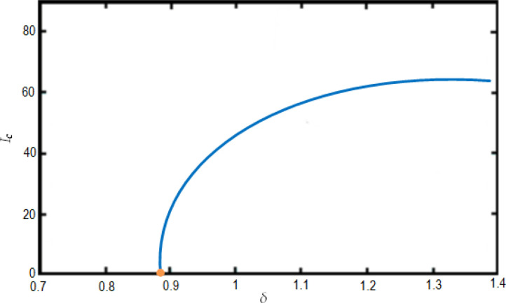
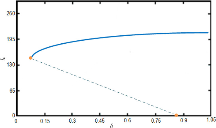
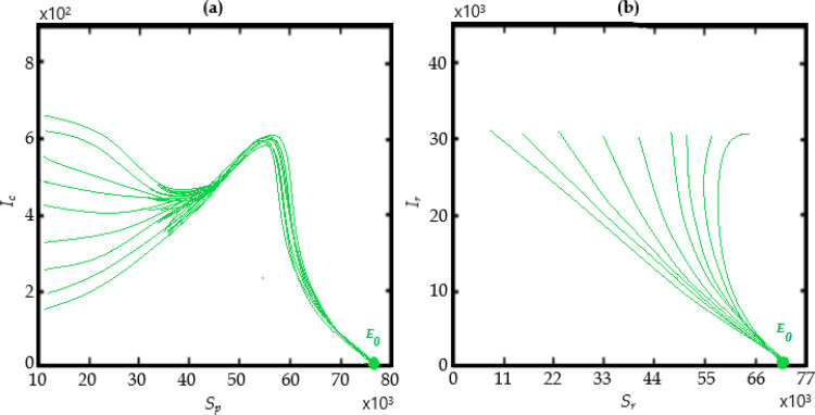
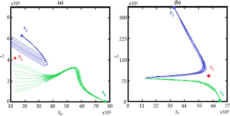
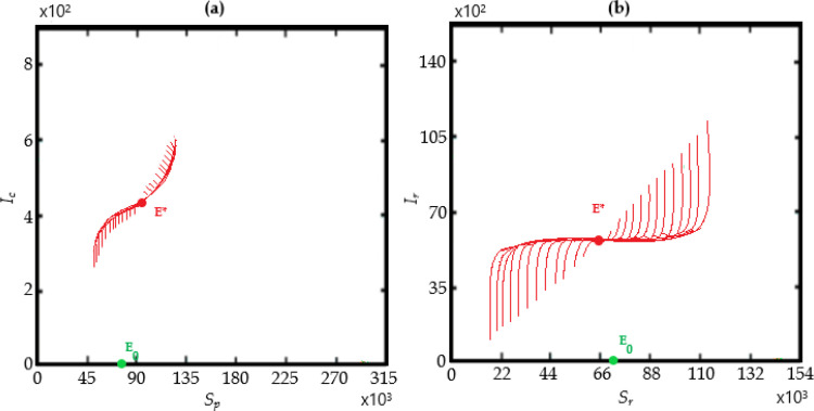
The bifurcation analysis are depicted in Figs. 11 and 12 showing condition for the model to have forward and backward bifurcations respectively. and show that the model contains a backward bifurcation under certain conditions. We also study different scenarios of stability and unstability state of equilibrium points (the DFE $E_0=(762224.14,0,70711.11,0)$ and the endemic equilibrium point) as shown in Fig. 13, Fig. 14, Fig. 15 . The globally stable DFE E ₀ is illustrated in Fig. 13 while a stable endemic equilibrium, namely $E_2=(1938.62,657.11,34941.36,36511.93),$ and an unstable endemic equilibrium $E_1=(13687.91,412.38,61442.11,8992.32)$ are shown in Fig. 12 when ${\beta }_r=0.07,\sigma =0.155({\mathcal{R}}_c=0.50167)$. Fig. 15 shows that there exists a globally stable endemic equilibrium $E^{*}=(96211.13,413.18,68644.21,6513.13)$ for the COVID-19 system (10) and an unstable DFE E ₀, when ${\beta }_r=1.60,\sigma =6.33\times {10}^{-13}({\mathcal{R}}_c=1.07121).$

Fig. 11.

Illustration of the forward bifurcation process from I_h versus $\delta =\sigma {\beta }_c$ for the COVID-19 system (10) with ${\beta }_r=0.03$ and also with ${\Lambda }_p=1000,{\Lambda }_r=2500,{\mu }_h=0.0131,{\mu }_c=0.035$ and ${\kappa }_c=199\times {10}^{-4}.$

Fig. 12.

Illustration of the backward bifurcation process from I_h versus $\delta =\sigma {\beta }_c$ for the COVID-19 system (10) with ${\beta }_r=0.05,$ and also with ${\Lambda }_p=1000,{\Lambda }_r=2500,{\mu }_h=0.0131,{\mu }_c=0.035$ and ${\kappa }_c=199\times {10}^{-4}.$

Fig. 13.

Existence of a globally stable disease-free equilibrium $E_0=(762224.14,0,70711.11,0)$ for the COVID-19 system (10) when ${\beta }_r=0.05,\sigma =0.217({\mathcal{R}}_c=0.33379).$

Fig. 14.

Existence for the COVID-19 system (10), of two stable equilibrium points: The DFE E₀, a stable endemic equilibrium $E_2=(1938.62,657.11,34941.36,36511.93),$ and an unstable endemic equilibrium $E_1=(13687.91,412.38,61442.11,8992.32)$ when ${\beta }_r=0.07,\sigma =0.155({\mathcal{R}}_c=0.50167).$

Fig. 15.

Existence of a globally stable endemic equilibrium $E^{*}=(96211.13,413.18,68644.21,6513.13)$ for the COVID-19 system (10) and an unstable DFE E₀, when ${\beta }_r=1.60,\sigma =6.33\times {10}^{-13}({\mathcal{R}}_c=1.07121).$

8. Endemic equilibria’s existence for combined HIV and COVID-19 model (1)

The endemic equilibrium, denoted by $E^{*}=(S_p^{*},I_c^{*},I_h^{*},I_{hc}^{*},S_r^{*},I_r^{*})$ is obtained by solving

$$\{\begin{array}{c}0={\Lambda }_p+\gamma I_c^{*}-({\lambda }_c^{*}+{\lambda }_h^{*}+{\mu }_h)S_p^{*},\hfill \\ 0={\lambda }_c^{*}{S}_p^{*}-(\epsilon {\lambda }_h^{*}+{\mu }_h+{\kappa }_c+\gamma )I_c^{*},\hfill \\ 0={\lambda }_h^{*}{S}_p^{*}+\varpi I_{hc}^{*}-(\theta {\lambda }_c^{*}+{\mu }_h+{\kappa }_h)I_h^{*},\hfill \\ 0=\epsilon {\lambda }_h^{*}{I}_c^{*}+\theta {\lambda }_c^{*}{I}_h^{*}-({\mu }_h+\tau {\kappa }_c+\nu {\kappa }_h+\varpi )I_{hc}^{*},\hfill \\ 0={\Lambda }_r-({\mu }_c+{\lambda }_r^{*})S_r^{*}\hfill \\ 0={\lambda }_r^{*}{S}_r^{*}-{\mu }_c{I}_r^{*},\hfill \end{array}$$ (21)

where ${\lambda }_c^{*},{\lambda }_h^{*}$ and ${\lambda }_r^{*}$ are respectively the forces of infection a steady-state reading as

$${\lambda }_c^{*}=\frac{{\beta }_c\sigma I_r^{*}}{N_p^{*}},N_p^{*}=S_p^{*}+I_c^{*}+I_h^{*}+I_{hc}^{*}$$

$${\lambda }_h^{*}=\frac{{\beta }_h(I_h^{*}+{\xi }_{hc}{I}_{hc}^{*})}{N_p^{*}},$$ (22)

$${\lambda }_r^{*}=\frac{{\beta }_r\sigma I_r^{*}}{N_r^{*}},N_r^{*}=S_r^{*}+I_r^{*}.$$

Hence after solving (21), we obtain

$$S_p^{*}=\frac{{\Lambda }_p({\mu }_h+{\kappa }_c+\gamma +\epsilon {\lambda }_h^{*})}{{\lambda }_c^{*}({\mu }_h+{\kappa }_c+\epsilon {\lambda }_h^{*})+({\lambda }_c^{*}+{\mu }_h)({\mu }_h+{\kappa }_c+\gamma +\epsilon {\lambda }_h^{*})}$$

$$I_c^{*}=\frac{{\Lambda }_p{\lambda }_c^{*}}{{\lambda }_c^{*}({\mu }_h+{\kappa }_c+\epsilon {\lambda }_h^{*})+({\lambda }_c^{*}+{\mu }_h)({\mu }_h+{\kappa }_c+\gamma +\epsilon {\lambda }_h^{*})}$$ (23)

$$I_h^{*}=\frac{{\Lambda }_p{\lambda }_h^{*}(({\mu }_h+\tau {\kappa }_c+\nu {\kappa }_h+\varpi )({\mu }_h+{\kappa }_c+\gamma +\epsilon {\lambda }_h^{*})+\varpi \epsilon {\lambda }_c^{*})}{A_1(\gamma ({\lambda }_h^{*}+{\mu }_h)+({\mu }_h+{\kappa }_c+\epsilon {\lambda }_h^{*})({\lambda }_h^{*}+{\lambda }_c^{*}+{\mu }_h))}$$

$$I_{hc}^{*}=\frac{{\Lambda }_p{\lambda }_h^{*}{\lambda }_c^{*}(\epsilon ({\mu }_h+{\kappa }_c+\epsilon {\lambda }_h^{*})+\theta ({\mu }_h+{\kappa }_c+\gamma +\epsilon {\lambda }_h^{*}))}{A_1(\gamma ({\lambda }_h^{*}+{\mu }_h)+({\mu }_h+{\kappa }_c+\epsilon {\lambda }_h^{*})({\lambda }_h^{*}+{\lambda }_c^{*}+{\mu }_h))}$$

$$S_r^{*}=\frac{{\Lambda }_r}{{\lambda }_r^{*}+{\mu }_c}$$

$$I_r^{*}=\frac{{\Lambda }_r{\lambda }_r^{*}}{{\mu }_c({\lambda }_r^{*}+{\mu }_c)}$$

with

$$A_1=\varpi ({\mu }_h+{\kappa }_h)+({\kappa }_h+\theta {\lambda }_c^{*}+{\mu }_h)(\tau {\kappa }_c+{\mu }_h+\nu {\kappa }_h).$$

After some transformations using the later system and the forces of infection (22), we obtain characteristic equations with the following roots: ${\lambda }_h^{*}=0,{\lambda }_c^{*}=0$ plus the roots of

$$K_1({\lambda }_h^{*},{\lambda }_c^{*})=0$$

and

$$K_2({\lambda }_h^{*},{\lambda }_c^{*})=0$$

where K ₁ and K ₂ are respectively complex polynomials of order two in ${\lambda }_c^{*}$ and order four in ${\lambda }_h^{*}$ with coefficients which are also complex polynomials of order two in ${\lambda }_h^{*}$ and order four in ${\lambda }_c^{*}$ respectively.

Hence the later results show that there are some values for both reproduction numbers ${\mathcal{R}}_c$ and ${\mathcal{R}}_h$ and therefore ${\mathcal{R}}_0$ for which the only obvious equilibrium point is the DFE. Similarly there some values for both reproduction numbers ${\mathcal{R}}_c$ and ${\mathcal{R}}_h$ and therefore ${\mathcal{R}}_0$ for which the full combined HIV and COVID-19 model (16) has either a HIV equilibrium point or a COVID-19 equilibrium point. Lastly, there some values for both reproduction numbers ${\mathcal{R}}_c$ and ${\mathcal{R}}_h$ and therefore ${\mathcal{R}}_0$ for which the combined HIV and COVID-19 model (16) a has a co-infection equilibrium point. Let us now study the COVID-19 global picture by numerically investigate the generalized version of the model (16).

9. Generalised COVID-19 model

we generalize the COVID-19 model (10) as

$$\{\begin{array}{c}{}^C{D}_t^{\alpha }\left(S_p\left(t\right)\right)={\Lambda }_p+\gamma I_c-({\lambda }_c+{\mu }_h)S_p,\hfill \\ {}^C{D}_t^{\alpha }\left(I_c\left(t\right)\right)={\lambda }_c{S}_p-({\mu }_h+{\kappa }_c+\gamma )I_c,\hfill \\ {}^C{D}_t^{\alpha }\left(S_r\left(t\right)\right)={\Lambda }_r-({\mu }_c+{\lambda }_r)S_r\hfill \\ {}^C{D}_t^{\alpha }\left(I_r\left(t\right)\right)={\lambda }_r{S}_r-{\mu }_c{I}_r,\hfill \end{array}$$ (24)

with the force of infection λ_c and λ_r reading respectively as

$${\lambda }_c=\frac{{\beta }_c\sigma I_r}{N_p},$$

and

$${\lambda }_r=\frac{{\beta }_r\sigma I_r}{N_r},$$

and where ${}^C{D}_t^{\alpha }$ is the classical Caputo fractional derivative that, for the order α, and for any t > 0, is defined as

$${}^C{D}_t^{\alpha }S\left(t\right)=I^{1-\alpha }\frac{d}{dt}S\left(t\right),0<\alpha \le 1,$$ (25)

where $-\infty \le a<t,b>a$ and $S:(a,b)⟶\mathbb{R}$ is a real and locally integrable function and

$$I^{\alpha }S\left(t\right)=\frac{1}{\Gamma \left(\alpha \right)}{\int }_a^t\frac{S\left(\tau \right)}{{(t-\tau )}^{1-\alpha }}d\tau ,$$ (26)

is the fractional integral of order α associated to ${}^C{D}_t^{\alpha }.$

In order to conveniently solve the combined fractional and fractal system (24), it is important to associate it with the following initial conditions:

$$S_p\left(0\right)=\widetilde{S_p}\left(S_p\right),I_c\left(0\right)=\widetilde{I_c}\left(I_c\right),S_r\left(0\right)=\widetilde{S_r}\left(S_r\right),I_r\left(0\right)=\widetilde{I_r}\left(I_r\right).$$ (27)

We now transform the system (24)-(27) so that it takes a compact form of the Legendre wavelets approach as described in [19], [20]. So consider

$$\{\begin{array}{c}{}^C{D}_t^{\alpha }\left(S_p\left(t\right)\right)={}^T{M}_m^1{\Psi }_m\left(t\right),\hfill \\ {}^C{D}_t^{\alpha }\left(I_c\left(t\right)\right)={}^T{M}_m^2{\Psi }_m\left(t\right),\hfill \\ {}^C{D}_t^{\alpha }\left(S_r\left(t\right)\right)={}^T{M}_m^3{\Psi }_m\left(t\right)\hfill \\ {}^C{D}_t^{\alpha }\left(I_r\left(t\right)\right)={}^T{M}_m^4{\Psi }_m\left(t\right).\hfill \end{array}$$ (28)

Here Ψ_m(t) is the matrix whose elements define the Legendre wavelets given as

$${\psi }_{nm}\left(t\right)=\{\begin{array}{cc}{2}^{k/2}\sqrt{2m+1}{L}_m^{*}(2^{k}t-n)),\hfill & \text{if}t\in \left[{\displaystyle \frac{n}{2^k},\frac{n+1}{2^k}}\right];\hfill \\ 0,\hfill & \text{elsewhere}.\hfill \end{array}$$ (29)

with $L_m^{*}$ the shifted Legendre polynomial defined on [0, 1] as $L_m^{*}\left(t\right)=L_m(2t-1),{\left(L_m(2t-1)\right)}_m$ being the family

$$\begin{array}{ccc}\hfill L_0& =& 1,L_1=x,L_{m+1}\left(x\right)=\frac{1+2m}{m+1}x{L}_m\left(x\right)-\frac{m}{1+m}{L}_{m-1}\left(x\right),\hfill \\ \hfill m& =& 1,2,\cdots .\hfill \end{array}$$ (30)

^T M ¹, ^T M ², ^T3 and ^T M ⁴ are the transpose of the matrices M ¹, M ², M ³ and M ⁴ respectively. Associating the initial conditions yields

$$\{\begin{array}{c}{S}_p\left(t\right)\approx {}^T{M}_m^1{Q}_{m\times m}^{\alpha }{\Psi }_m\left(t\right)+\widetilde{S_p},\hfill \\ I_c\left(t\right)\approx {}^T{M}_m^2{Q}_{m\times m}^{\alpha }{\Psi }_m\left(t\right)+\widetilde{I_c},\hfill \\ S_r\left(t\right)\approx {}^T{M}_m^3{Q}_{m\times m}^{\alpha }{\Psi }_m\left(t\right)+\widetilde{S_r}\hfill \\ I_r\left(t\right)\approx {}^T{M}_m^4{Q}_{m\times m}^{\alpha }{\Psi }_m\left(t\right)+\widetilde{I_r},\hfill \end{array}$$ (31)

where $Q_{m\times m}^{\alpha }$ is the Legendre operational matrix of integration and the subscript m denotes its dimension. We know that [19], [20], Legendre wavelets can be expanded into an m-term form as

$${\Psi }_m\left(t\right)={{\rm Y}}_{m\times m}{A}_m\left(t\right),$$ (32)

where $A_m\left(t\right){=}^T[a_1\left(t\right),a_2\left(t\right),\cdots ,a_m\left(t\right)]$ is the Block Pulse Functions so that

$$\begin{array}{c}\hfill a_k\left(t\right)=\{\begin{array}{cc}1,\hfill & \text{if}t\in [\frac{k-1}{m},\frac{k}{m}];\hfill \\ 0,\hfill & \text{elsewhere}.\hfill \end{array}\end{array}$$ (33)

for each $k=1,2,\cdots m,$ and Υ the Legendre wavelet matrix

$${{\rm Y}}_{m\times m}=[{\Psi }_m\left(\frac{1}{2m}\right){\Psi }_m\left(\frac{3}{2m}\right)\cdots {\Psi }_m\left(\frac{2m-1}{2m}\right)]$$

Now the substitution of (32) into system (31) leads to

$$\{\begin{array}{c}{S}_p\left(t\right)\approx {}^T{M}_m^1{Q}_{m\times m}^{\alpha }{{\rm Y}}_{m\times m}{A}_m\left(t\right)+\left[{\widetilde{S_p}}_i\right]A_m\left(t\right),\hfill \\ I_c\left(t\right)\approx {}^T{M}_m^2{Q}_{m\times m}^{\alpha }{{\rm Y}}_{m\times m}{A}_m\left(t\right)+\left[{\widetilde{I_c}}_i\right]A_m\left(t\right),\hfill \\ S_r\left(t\right)\approx {}^T{M}_m^3{Q}_{m\times m}^{\alpha }{{\rm Y}}_{m\times m}{A}_m\left(t\right)+\left[{\widetilde{S_r}}_i\right]A_m\left(t\right),\hfill \\ I_r\left(t\right)\approx {}^T{M}_m^4{Q}_{m\times m}^{\alpha }{{\rm Y}}_{m\times m}{A}_m\left(t\right)+\left[{\widetilde{I_r}}_i\right]A_m\left(t\right).\hfill \end{array}$$ (34)

Where

$$\left[{\widetilde{S_p}}_i\right]=[{\widetilde{S_p}}_1,{\widetilde{S_p}}_2,\cdots ,{\widetilde{S_p}}_m],\left[{\widetilde{I_c}}_i\right]=[{\widetilde{I_c}}_1,{\widetilde{I_c}}_2,\cdots ,{\widetilde{I_c}}_m]$$

$$\left[{\widetilde{S_r}}_i\right]=[{\widetilde{S_r}}_1,{\widetilde{S_r}}_2,\cdots ,{\widetilde{S_r}}_m],\left[{\widetilde{I_r}}_i\right]=[{\widetilde{I_r}}_1,{\widetilde{I_r}}_2,\cdots ,{\widetilde{I_r}}_m].$$

Now let

$${}^T{M}_m^i{Q}_{m\times m}^{\alpha }{{\rm Y}}_{m\times m}={\mathcal{M}}_{1\times m}^{\alpha ,i}=[m_1^{\alpha ,i},m_2^{\alpha ,i},\cdots ,m_m^{\alpha ,i}]$$ (35)

Now Using the collocations points $t_i=\frac{2i-1}{2^{k+1}N},i=1,2,3,\cdots ,m$ $N\in \mathbb{N},$ to disperse t, the substitution of (34) and (35) into system (24) and lead to

$$\{\begin{array}{c}{}^T{M}_m^1{{\rm Y}}_{m\times m}={\Lambda }_p[1,1\cdots ,1]+\gamma [m_1^{\alpha ,2},m_2^{\alpha ,2},\cdots ,m_m^{\alpha ,2}]-({\lambda }_c+{\mu }_h)\hfill \\ [m_1^{\alpha ,1},m_2^{\alpha ,1},\cdots ,m_m^{\alpha ,1}]+[{\widetilde{S_p}}_1,{\widetilde{S_p}}_2,\cdots ,{\widetilde{S_p}}_m],\hfill \\ {}^T{M}_m^2{{\rm Y}}_{m\times m}={\lambda }_c[m_1^{\alpha ,1},m_2^{\alpha ,1},\cdots ,m_m^{\alpha ,1}]-({\mu }_h+{\kappa }_c+\gamma )\hfill \\ [m_1^{\alpha ,2},m_2^{\alpha ,2},\cdots ,m_m^{\alpha ,2}]+[{\widetilde{I_c}}_1,{\widetilde{I_c}}_2,\cdots ,{\widetilde{I_c}}_m]\hfill \\ {}^T{M}_m^3{{\rm Y}}_{m\times m}={\Lambda }_r[1,1\cdots ,1]-({\mu }_c+{\lambda }_r)[m_1^{\alpha ,3},m_2^{\alpha ,3},\cdots ,m_m^{\alpha ,3}]\hfill \\ [{\widetilde{S_r}}_1,{\widetilde{S_r}}_2,\cdots ,{\widetilde{S_r}}_m]\hfill \\ {}^T{M}_m^4{{\rm Y}}_{m\times m}={\lambda }_r[m_1^{\alpha ,3},m_2^{\alpha ,3},\cdots ,m_m^{\alpha ,3}]-{\mu }_c[m_1^{\alpha ,4},m_2^{\alpha ,4},\cdots ,m_m^{\alpha ,4}]\hfill \\ [{\widetilde{I_r}}_1,{\widetilde{I_r}}_2,\cdots ,{\widetilde{I_r}}_m]\hfill \end{array}$$ (36)

Hence we obtain this non-linear system equations with 4m unknown coefficients $m_k^{\alpha ,i},1\le i\le 4,1\le k\le m$ which are easily found using Newton iteration method. Then exploiting model (31), leads the south numerical solution (S_p(t), I_c(t), S_r(t), I_r(t)).

10. Numerical simulations with some known COVID-19 data

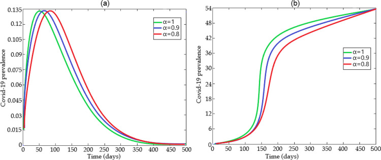
We can implement in this section the numerical scheme presented above using some data recently given in the literature and summarized in the Table 2 . The numerical simulations for the behavior of the COVID-19 prevalence for the generalized model (24), performed for certain values of α are depicted in Fig. 16 (a) when ${\mu }_c=0.059$ and ${\mathcal{R}}_c=0.64103$ and Fig. 16 (b) when ${\mu }_c=0.019$ and ${\mathcal{R}}_c=5.70103.$

Table 2.

Description and values for the parameters [21], [22].

Parameters	Descriptions	Estimated baseline values
Λp	Recruitment rate of people population	1000
Λr	Recruitment rate of susceptible animals	2500
βc	Human transmission probability for COVID-19	Variable
βr	Animal transmission probability for COVID-19	0.05–1.6
σ	Per capita vector-to-host contact rate	$6.33\times {10}^{-3}$–0.217
μh	Natural death rate in humans	0.0131
μc	Natural mortality rate of animals	0.035
κc	COVID-19 mortality rate	$199\times {10}^{-4}$
γ	People recovery rate from COVID-19	0.005
ϖ	HIV People recovery rate from COVID-19	0.002
θ, ν	Regulation parameters	1.0021, 1.002
ε, τ, ξhc	Regulation parameters	1,001, 1.001, 1.005,

Fig. 16.

Some predicted COVID-19 prevalence using the generalized model (24) for certain values of α over 500 days using Table 2 and (a) when ${\mu }_c=0.059$ and ${\mathcal{R}}_c=0.64103$ and (b) when ${\mu }_c=0.019$ and ${\mathcal{R}}_c=5.70103$.

11. Concluding remarks

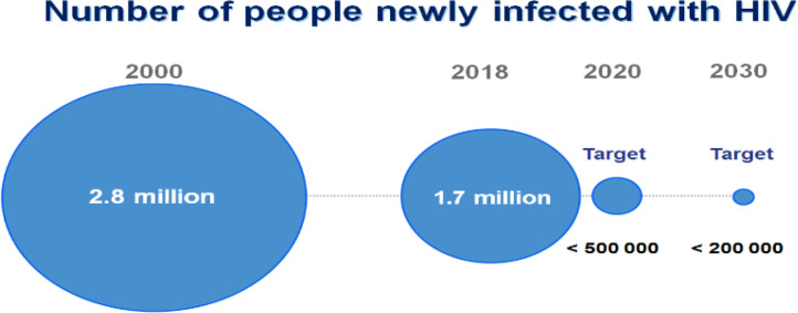
As shown in Fig. 1, Fig. 8 and Fig. 9 , the numbers of victims and fatalities due to HIV and the new coronavirus remain a fateful scourge around the world. The combination of both will certainly be explosive for most affected countries. We especially think of southern hemisphere countries getting out the summer and moving into the winter season. It is urgent for those countries (like South Africa and Chile) to be alerted while it is still time to react efficiently. Indeed, the world has ignored the first alert made before the pandemic, by the young and now late Chinese doctor Li Wenliang and this is paper serves as a COVID-19 alert for southern hemisphere countries like Chile and South Africa that are moving into the winter season and seeing to be heavily hit by the pandemic. As winter moved to the southern hemisphere, we also observed the epicenter of the new coronavirus shifting there to Brazil, which shares similar features (such as Favellas, townships, poverty, promiscuity) with South Africa and Chile. We have then used a generalized simple mathematical model of HIV-COVID-19 together with graphs, curves and tables to compare the pandemic situation in countries that were once the epicenter of the disease, such as China, Italy, Spain, United Kingdom and United States of America. We managed to show conditions for existence of stable equilibria and of different bifurcation (forward and backward) scenarios for the model. The fractional (generalized) COVID-19 model has been solved numerically and a predicted prevalence for the COVID-19 has been provided. There is a ground to be concerned for southern hemisphere countries now since it happens that all those countries that were once epicenter, were in their winter season during their status of epicenter of the COVID-19 and opted to ease the lockdown only after the peak of the disease was reached. The epicenter is now in Brazil, in full winter season, and we observe its health system and emergency services overcrowded by a large number of COVID-19 patients and deaths. Recent data show an increasing number of infections in Chile and South Africa. The combination with HIV cannot help. Moreover, still far from seeing the disease reaching its peak in the country, South Africa who has just enter into the winter season, opted to reopen the country’s activities and schools. This is exactly the opposite of what was observed in western countries. Recall that South Africa stands now as the most COVID-19 affected country in Africa and is it going to be the next epicenter in weeks to come when winter conditions favorable to the spread of the new coronavirus will be comfily installed? The answer is certainly affirmative seeing the social conditions in townships all over the country. The country has however started imposing social distanciation, wearing a face mask in public services, hiring of more health workers and targeted community tests. Will this be enough, as the country chose to reopen most of it economic sectors as from the 1 June 2020, which coincides with beginning of its winter season, we can now ask whether the lockdown that started on the 26 March 2020 was at the right moment. The coming months will tell us. Lastly, another worrying alert is the fact that winter is still going to move to Europe and we may see again the epicenter shifting towards the north, unless a cure or vaccine is found by then. Again the future months will tell us.

Fig. 9.

Illustration of the yearly increase of HIV cases worldwide the WHO [5].

CRediT authorship contribution statement

Emile F. Doungmo Goufo: Conceptualization, Methodology, Writing - original draft. Yasir Khan: Data curation. Qasim Ali Chaudhry: Writing - original draft, Writing - review & editing, Investigation.

Declaration of Competing Interest

The authors declare that they have no known competing financial interests or personal relationships that could have appeared to influence the work reported in this paper.

References

- 1.Radusin M. The spanish flu, part ii: the second and third wave. Vojnosanit Pregl. 2012;69(10):917–927. [PubMed] [Google Scholar]
- 2.Green A. Li wenliang. Lancet. 2020;395(10225):682. [Google Scholar]
- 3.Sajadi M.M., Habibzadeh P., Vintzileos A., Shokouhi S., Miralles-Wilhelm F., Amoroso A.. Temperature and latitude analysis to predict potential spread and seasonality for covid-19. Available at SSRN 35503082020;. [DOI] [PMC free article] [PubMed]
- 4.W.H. Organization, et al. Coronavirus disease 2019 (covid-19): situation report, 73. https://www.whoint/emergencies/diseases/novel-coronavirus-2019/situation-reports, consulted 2 June 2020.
- 5.W. H. Organization, et al. Number of people newly infected with Hiv. https://www.whoint/gho/hiv/epidemicstatus/incidence/en/, consulted 2 June 2020.
- 6.Pereira R.J., do Nascimento G.N.L., Gratão L.H.A., Pimenta R.S. The risk of covid19 transmission in favelas and slums in brazil. Public Health. 2020 doi: 10.1016/j.puhe.2020.04.042. [DOI] [PMC free article] [PubMed] [Google Scholar]
- 7.S.S. Africa S.S.. Mid-year population estimates: Sa population reaches 58,8 million. Available at http://www.statssagovza/publications/P0302/P03022019pdf, consulted 2 June 2020.
- 8.Atangana A., Goufo E.F.D. On the mathematical analysis of ebola hemorrhagic fever: deathly infection disease in west african countries. Biomed Res Int. 2014;2014 doi: 10.1155/2014/261383. [DOI] [PMC free article] [PubMed] [Google Scholar]
- 9.Atangana A., Goufo D., Franc E. Computational analysis of the model describing Hiv infection of cd4. Biomed Res Int. 2014;2014 doi: 10.1155/2014/618404. [DOI] [PMC free article] [PubMed] [Google Scholar]
- 10.Goufo D., Franc E., Oukouomi Noutchie S.C., Mugisha S. Abstract and applied analysis. Vol. 2014. Hindawi; 2014. A fractional SEIR epidemic model for spatial and temporal spread of measles in metapopulations. [Google Scholar]
- 11.Goufo E.F.D., Maritz R., Munganga J. Some properties of the Kermack-Mckendrick epidemic model with fractional derivative and nonlinear incidence. Adv Differ Equ. 2014;2014(1):278. [Google Scholar]
- 12.Goufo E.D., Maritz R. A note on ebola’s outbreak and human migration dynamic. J Hum Ecol. 2015;51(3):257–263. [Google Scholar]
- 13.Goufo E.F.D., Pene M.K., Mugisha S. Stability analysis of epidemic models of ebola hemorrhagic fever with non-linear transmission. J Nonlinear Sci Appl. 2016;9(6) [Google Scholar]
- 14.Khan M.A., Iqbal N., Khan Y., Alzahrani E. A biological mathematical model of vector-host disease with saturated treatment function and optimal control strategies. Math Biosci Eng. 2020;17(4):3972. doi: 10.3934/mbe.2020220. [DOI] [PubMed] [Google Scholar]
- 15.Khan M.A., Shah K., Khan Y., Islam S. Mathematical modeling approach to the transmission dynamics of pine wilt disease with saturated incidence rate. Int J Biomath. 2018;11(3):1850035. [Google Scholar]
- 16.Mukandavire Z., Gumel A.B., Garira W., Tchuenche J.M.. Mathematical analysis of a model for Hiv-malaria co-infection2009;. [DOI] [PubMed]
- 17.Van den Driessche P., Watmough J. Reproduction numbers and sub-threshold endemic equilibria for compartmental models of disease transmission. Math Biosci. 2002;180(1):29–48. doi: 10.1016/s0025-5564(02)00108-6. [DOI] [PubMed] [Google Scholar]
- 18.Wiggins S. Vol. 2. Springer Science & Business Media; 2003. Introduction to applied nonlinear dynamical systems and chaos. [Google Scholar]
- 19.Razzaghi M., Yousefi S. The legendre wavelets operational matrix of integration. Int J Syst Sci. 2001;32(4):495–502. [Google Scholar]
- 20.Chen Y., Ke X., Wei Y. Numerical algorithm to solve system of nonlinear fractional differential equations based on wavelets method and the error analysis. Appl Math Comput. 2015;251:475–488. [Google Scholar]
- 21.Resmawan R., Yahya L. Sensitivity analysis of mathematical model of coronavirus disease (covid-19) transmission. CAUCHY. 2020;6(2):91–99. [Google Scholar]
- 22.Khan M.A., Atangana A. Modeling the dynamics of novel coronavirus (2019-ncov) with fractional derivative. Alexandria Eng J. 2020 [Google Scholar]