Computation of Electromagnetic Properties of Molecular Ensembles

Abstract

We outline a methodology for efficiently computing the electromagnetic response of molecular ensembles. The methodology is based on the link that we establish between quantum‐chemical simulations and the transfer matrix (T‐matrix) approach, a common tool in physics and engineering. We exemplify and analyze the accuracy of the methodology by using the time‐dependent Hartree‐Fock theory simulation data of a single chiral molecule to compute the T‐matrix of a cross‐like arrangement of four copies of the molecule, and then computing the circular dichroism of the cross. The results are in very good agreement with full quantum‐mechanical calculations on the cross. Importantly, the choice of computing circular dichroism is arbitrary: Any kind of electromagnetic response of an object can be computed from its T‐matrix. We also show, by means of another example, how the methodology can be used to predict experimental measurements on a molecular material of macroscopic dimensions. This is possible because, once the T‐matrices of the individual components of an ensemble are known, the electromagnetic response of the ensemble can be efficiently computed. This holds for arbitrary arrangements of a large number of molecules, as well as for periodic or aperiodic molecular arrays. We identify areas of research for further improving the accuracy of the method, as well as new fundamental and technological research avenues based on the use of the T‐matrices of molecules and molecular ensembles for quantifying their degrees of symmetry breaking. We provide T‐matrix‐based formulas for computing traditional chiro‐optical properties like (oriented) circular dichroism, and also for quantifying electromagnetic duality and electromagnetic chirality. The formulas are valid for light‐matter interactions of arbitrarily‐high multipolar orders.

We outline a methodology for efficiently computing the electromagnetic response of molecular ensembles. Instead of performing quantum‐mechanical simulations of the entire ensemble, we combine the quantum‐mechanical simulations of single molecules with the transfer matrix (T‐matrix) approach, a common tool in physics and engineering. We show that the T‐matrix calculations agree very well with the full quantum‐mechanical calculations. We also show how the methodology can be used to predict experimental measurements on a molecular material of macroscopic dimensions.

1. Introduction

Nanoscience is an interdisciplinary endeavor. The study of matter, radiation, and their interaction at tiny spatial scales involves many different fields in physics and chemistry. Moreover, engineering is eventually needed to convert the scientific advances into technological ones. Each discipline has its own methods, which complicates cross‐talk and hinders progress. The molecular‐based design of discrete objects and bulk materials for specific electromagnetic functions is a prominent example of interdisciplinary work where chemistry, physics, and engineering need to come together. It is also an example of one of the main challenges in nanotechnology: Scale heterogeneity.1 It is hence desirable to develop approaches that connect methodologies across the different disciplines and length scales in nano and mesoscopic science and technology. One of the objectives of such approaches, which can open up opportunities in computational material science, is to predict the observable electromagnetic properties of macroscopic functional devices from descriptions at the molecular level.

At the smallest length scales, quantum‐mechanical simulation methods based on, for example, time‐dependent density functional theory (TD‐DFT), time‐dependent Hartree‐Fock theory (TD‐HF), or linear‐response coupled‐cluster theory (LR‐CC) are used in computational chemistry to obtain the electromagnetic response of single molecules.2, 3, 4, 5 One limitation of this kind of simulations is that their computational complexity renders them impractical when the system size goes beyond 10⁴ atoms.6, 7 In physics and engineering, the transfer matrix (T‐matrix) approach8 is a very common tool for computing the electromagnetic responses of single and composite objects. The T‐matrix of an object is equivalent to its scattering matrix and contains all the information about its electromagnetic response. Any electromagnetic property can be computed from it. Given the T‐matrices of the individual constituents, the joint response of a composite system like random media, and periodic or aperiodic arrays, can be computed efficiently (see the references in [9, Secs. 2.6 and 2.7]). For example, state‐of‐the‐art T‐matrix codes can handle ensembles of tens of thousands of individual objects.10 The computation of the T‐matrices of individual objects requires a basic model for light‐matter interactions. The model is typically the macroscopic Maxwell equations featuring the constitutive relations: Electric permittivity, magnetic permeability, etc. The main limitation of this approach is that at small enough scales, namely below 10 nm [11,Chap. 6.6], the effective field description implicit in the constitutive relations ceases to be a good approximation.

In this article, we propose a methodology for efficiently computing the electromagnetic response of molecular ensembles. The methodology is based on linking quantum‐mechanical molecular simulations to the T‐matrix approach. The former provide the basic model for the latter. Their combination solves both the scalability issue of molecular simulations and the failure of macroscopic electromagnetism at the nano and meso scales. In Sec. 2 we show how to build the T‐matrix of a molecule using the dynamic polarizabilities obtained through quantum‐mechanical molecular simulations. We also derive formulas to compute the oriented circular dichroism (OCD) and rotationally averaged circular dichroism (CD) from the T‐matrix. The expressions are not limited to the dipolar approximation: They are valid for arbitrarily high multipolar orders. These expressions are hence useful for molecular ensembles whose sizes prevent the use of the dipolar approximation. In Sec. 3 we start from single‐molecule quantum‐mechanical simulations performed with the turbomole program package,12, 13 and apply the proposed methodology by first computing the T‐matrix and then the CD of a cross‐like arrangement of four identical molecules. We compare the results with the full quantum calculation and find a very good agreement. It must be noted that the full quantum calculation of the cross pushes current computational means to their limits, and that somewhat larger molecular assemblies cannot be fully quantum mechanically analyzed in a fair amount of time. In sharp contrast, the electromagnetic response of assemblies much larger than the cross can be efficiently computed with the proposed methodology. We put forward a modification of the basic methodology which improves its accuracy: The quantum‐mechanical computation of the polarizability tensors of a given individual molecule is done taking into account the electrostatic potential created by the other molecules in the ensemble. We identify aggregation effects at the frequencies where the disagreement between the T‐matrix‐based calculations and the full quantum‐mechanical reference is larger, which constitutes a topic of future research. Section 4 contains an example of the use of the methodology for the prediction of experimental measurements on a molecular material of macroscopic size: A chiral surface‐anchored metal‐organic framework (SURMOF) on a substrate. Before the conclusion, we discuss in Sec. 5 how some theoretical and technological research avenues related to the quantification of symmetry breaking open up once the T‐matrices of molecules and molecular ensembles become available. We also provide formulas to quantify two properties that have been recently shown to be fundamentally relevant to chiral interactions: Electromagnetic chirality and electromagnetic duality.

2. Using the T‐Matrix Techniques for Molecules

We start by connecting two different settings for describing light‐matter interactions at the molecular level: The electromagnetic polarizability tensor and the T‐matrix. We assume that the molecule is immersed in an isotropic and homogeneous medium, and approximately centered at position ${\mathbf{r}}_0$ . The molecule is illuminated by an incident electromagnetic field, with which it interacts. A re‐radiated (scattered) field results from the interaction. We restrict the following treatment to linear light‐matter interactions that do not change the frequency of the incident field. That is, given the decomposition of the incident field into harmonic components with $\exp \left(-i\omega t\right)$ time dependency, each component will only cause the molecule to generate a scattered field of the same frequency ω. We allow the electric permittivity ϵ and magnetic permeability μ of the surrounding medium to be frequency dependent $\{{ϵ}^{\omega },{\mu }^{\omega }\}$ . We also assume that the dimensions of the molecule are much smaller than any of the wavelengths contained in the incident field. Under these conditions, there is a very common setting for modeling the light‐matter interaction (see e. g. [14, Eq. (6)] and [15, Sec. 2]): The scattered fields produced by the molecule at each frequency ω are due to the radiation of an electric dipole moment ${\mathbf{p}}^{\omega }$ and a magnetic dipole moment ${\mathbf{m}}^{\omega }$ which are induced in the molecule by the incident electric and magnetic fields at the point ${\mathbf{r}}_0:$ $\left\{{\mathbf{E}}^{\omega }\left({\mathbf{r}}_0\right),{\mathbf{H}}^{\omega }\left({\mathbf{r}}_0\right)\right\}$ . The effect of the molecule is then completely characterized by a complex‐valued 6×6 matrix, which we here decompose in its four 3×3 blocks using an obvious naming convention:

$${\displaystyle \left[\begin{array}{c}{\mathbf{p}}^{\omega }\\ {\mathbf{m}}^{\omega }\end{array}\right]=\left[\begin{array}{cc}{\underset{\_}{\underset{\_}{\alpha }}}_{pE}^{\omega }& {\underset{\_}{\underset{\_}{\alpha }}}_{pH}^{\omega }\\ {\underset{\_}{\underset{\_}{\alpha }}}_{mE}^{\omega }& {\underset{\_}{\underset{\_}{\alpha }}}_{mH}^{\omega }\end{array}\right]\left[\begin{array}{c}{\mathbf{E}}^{\omega }\left({\mathbf{r}}_0\right)\\ {\mathbf{H}}^{\omega }\left({\mathbf{r}}_0\right)\end{array}\right].}$$ (1)

From now on, we choose the origin of the coordinate axes at ${\mathbf{r}}_0$ so that ${\mathbf{r}}_0=(0,0,0)$ . SI units are assumed throughout, and the $\exp \left(-i\omega t\right)$ factors are suppressed.

A more general formalism for the study of light‐matter interactions is the T‐matrix setting. The T‐matrix of an object relates the incident and scattered fields in the following way. First, a complete basis for free electromagnetic fields in the surrounding medium is chosen. The most common choice is the multipolar fields of well defined parity.9 This is the most convenient option for our initial purposes. Each multipolar field is characterized by its frequency ω, its total angular momentum squared $j(j+1)$ with $j=1$ (dipole), 2 (quadrupole), …, its angular momentum along one chosen axis $m=[-j,-j+1,...,j-1,j]$ , its parity or electric/magnetic character, and, for the T‐matrix formalism, its incident or scattered character. Scattered multipoles are purely outgoing, meet the radiation condition at infinity, and are singular at the origin, while incident multipoles do not have singularities, and are of a mixed incoming and outgoing character. Using this multipolar basis, each frequency component of the incident electric and magnetic fields can be written as

$${\displaystyle {\mathbf{E}}^{\omega }\left(\mathbf{r}\right)=\sum _{j=1}^{\infty }\sum _{m=-j}^j\left[a_{jm}^{\omega }{\mathbf{N}}_{jm}^{\omega }\left(\mathbf{r}\right)+b_{jm}^{\omega }{\mathbf{M}}_{jm}^{\omega }\left(\mathbf{r}\right)\right],i{Z}^{\omega }{\mathbf{H}}^{\omega }\left(\mathbf{r}\right)=\sum _{j=1}^{\infty }\sum _{m=-j}^j\left[b_{jm}^{\omega }{\mathbf{N}}_{jm}^{\omega }\left(\mathbf{r}\right)+a_{jm}^{\omega }{\mathbf{M}}_{jm}^{\omega }\left(\mathbf{r}\right)\right],}$$ (2)

where $\left\{a_{jm}^{\omega },b_{jm}^{\omega }\right\}$ are complex coefficients, ${\mathbf{N}}_{jm}^{\omega }\left(\mathbf{r}\right)$ are regular electric multipolar fields, ${\mathbf{M}}_{jm}^{\omega }\left(\mathbf{r}\right)$ are regular magnetic multipolar fields, $Z^{\omega }=\sqrt{{\mu }^{\omega }/{ϵ}^{\omega }}$ , and the second line follows from the first by first using one of Maxwell's equations to show that $i{Z}_{\omega }{\mathbf{H}}^{\omega }\left(\mathbf{r}\right)=\nabla \times {\mathbf{E}}^{\omega }\left(\mathbf{r}\right)/k^{\omega }$ , where $k^{\omega }=\omega \sqrt{{ϵ}^{\omega }{\mu }^{\omega }}$ , and then using the properties ([16, Eq. (3.8)]) $\nabla \times {\mathbf{M}}_{jm}^{\omega }\left(\mathbf{r}\right)=k^{\omega }{\mathbf{N}}_{jm}^{\omega }\left(\mathbf{r}\right)$ and $\nabla \times {\mathbf{N}}_{jm}^{\omega }\left(\mathbf{r}\right)=k^{\omega }{\mathbf{M}}_{jm}^{\omega }\left(\mathbf{r}\right)$ . More explicit expressions for ${\mathbf{M}}_{jm}^{\omega }\left(\mathbf{r}\right)$ and ${\mathbf{N}}_{jm}^{\omega }\left(\mathbf{r}\right)$ are given in Eq. (S3) of Supp. Inf. I. An expansion similar to Eq. (2), but featuring outgoing multipoles, holds for the scattered outgoing fields. We will denote by $c_{jm}^{\omega }$ the coefficients multiplying the scattered electric multipoles and by $d_{jm}^{\omega }$ the coefficients multiplying the magnetic ones. The T‐matrix is then a matrix that relates the coefficients of the incident field with those of the scattered field:

$${\displaystyle \left[\begin{array}{c}⋮\\ c_{jm}^{\omega }\\ ⋮\\ d_{jm}^{\omega }\\ ⋮\end{array}\right]={\underset{\_}{\underset{\_}{T}}}^{\omega }\left[\begin{array}{c}⋮\\ a_{jm}^{\omega }\\ ⋮\\ b_{jm}^{\omega }\\ ⋮\end{array}\right].}$$ (3)

Since the integer index j in Eq. (2) ranges from $j=1$ to infinity, the dimensionality of the vectors and matrix in Eq. (3) is infinite. Nevertheless, for any given object of finite size one can select a maximum multipolar order j _max beyond which the interaction of the object with the electromagnetic field can be neglected. The choice of a j _max makes the dimensions of the arrays in Eq. (3) finite. For molecules illuminated with propagating beams of visible or UV light, taking $j_{\max }=1$ (dipolar), or at most $j_{\max }=2$ (quadrupolar) should suffice.

In order to connect Eqs. (1) and (3), we now apply to Eq. (3) the restrictions contained in Eq. (1). We first consider the restriction that the scattered field is produced by dipole moments induced in the molecule. For each frequency and each parity there are three dipolar fields corresponding to $j=1$ and $m\in [-1,0,1]$ , for a total of 6 fields per frequency. Consequently, in the T‐matrix setting, the fields scattered by the molecule need to be restricted to belong to the subspace expanded by these six dipolar fields. Equation (1) also contains the restriction that the influence of the incident field is completely determined by its values at the origin. It turn sout that this also restricts the incident fields to be only dipolar. It is easy to see from the expressions of ${\mathbf{M}}_{jm}^{\omega }\left(\mathbf{r}\right)$ and ${\mathbf{N}}_{jm}^{\omega }\left(\mathbf{r}\right)$ at $\mathbf{r}=(0,0,0)$ (see Supp. Inf. I) that:

$${\displaystyle {\mathbf{E}}^{\omega }\left(0\right)=\left[\sum _{m=-1}^1{a}_{1m}^{\omega }{\mathbf{N}}_{1m}^{\omega }\left(0\right)\right],i{Z}^{\omega }{\mathbf{H}}^{\omega }\left(0\right)=\left[\sum _{m=-1}^1{b}_{1m}^{\omega }{\mathbf{N}}_{1m}^{\omega }\left(0\right)\right].}$$ (4)

Therefore, we can again write a 6×6 linear relationship, this time in the T‐matrix setting, which we also decompose into 3×3 blocks:

$${\displaystyle \left[\begin{array}{c}{c}_{1-1}^{\omega }\\ c_{10}^{\omega }\\ c_{11}^{\omega }\\ d_{1-1}^{\omega }\\ d_{10}^{\omega }\\ d_{11}^{\omega }\end{array}\right]=\left[\begin{array}{cc}{\underset{\_}{\underset{\_}{T}}}_{NN}^{\omega }& {\underset{\_}{\underset{\_}{T}}}_{NM}^{\omega }\\ {\underset{\_}{\underset{\_}{T}}}_{MN}^{\omega }& {\underset{\_}{\underset{\_}{T}}}_{MM}^{\omega }\end{array}\right]\left[\begin{array}{c}{a}_{1-1}^{\omega }\\ a_{10}^{\omega }\\ a_{11}^{\omega }\\ b_{1-1}^{\omega }\\ b_{10}^{\omega }\\ b_{11}^{\omega }\end{array}\right],}$$ (5)

where the subscripts in the block labels refer to the multipolar fields of Eq. (2).

The models in Eqs. (1) and (5) are physically equivalent. We show in Supp. Inf. I that the one‐to‐one relationship between the two 6×6 matrices is:

$${\displaystyle \left[\begin{array}{cc}{\underset{\_}{\underset{\_}{T}}}_{NN}^{\omega }& {\underset{\_}{\underset{\_}{T}}}_{NM}^{\omega }\\ {\underset{\_}{\underset{\_}{T}}}_{MN}^{\omega }& {\underset{\_}{\underset{\_}{T}}}_{MM}^{\omega }\end{array}\right]=\frac{i{c}^{\omega }{Z}^{\omega }{\left(k^{\omega }\right)}^3}{6\pi }\left[\begin{array}{cc}\underset{\_}{\underset{\_}{C}}\left({\underset{\_}{\underset{\_}{\alpha }}}_{pE}^{\omega }\right){\underset{\_}{\underset{\_}{C}}}^{-1}& \underset{\_}{\underset{\_}{C}}\left(-i{\underset{\_}{\underset{\_}{\alpha }}}_{pH}^{\omega }/Z^{\omega }\right){\underset{\_}{\underset{\_}{C}}}^{-1}\\ \underset{\_}{\underset{\_}{C}}\left(i{\underset{\_}{\underset{\_}{\alpha }}}_{mE}^{\omega }/c^{\omega }\right){\underset{\_}{\underset{\_}{C}}}^{-1}& \underset{\_}{\underset{\_}{C}}\left({\underset{\_}{\underset{\_}{\alpha }}}_{mH}^{\omega }/\left(c^{\omega }{Z}^{\omega }\right)\right){\underset{\_}{\underset{\_}{C}}}^{-1}\end{array}\right],}$$ (6)

where $c^{\omega }=1/\sqrt{{ϵ}^{\omega }{\mu }^{\omega }}$ is the frequency‐dependent speed of light in the surrounding medium, and $\underset{\_}{\underset{\_}{C}}$ is the 3×3 unitary change of basis matrix that goes from the Cartesian to the spherical basis [see Eq. (S8)]. This change of basis is needed in the most common case where Eq. (1) is expressed in the Cartesian basis. That is: ${\mathbf{p}}^{\omega }=[p_x^{\omega },p_y^{\omega },p_z^{\omega }]$ , ${\mathbf{E}}^{\omega }=[E_x^{\omega },E_y^{\omega },E_z^{\omega }]$ , etc. …. On the other hand, Eq. (5) is an expression related to the spherical basis.

Equation (6) connects the two settings and allows to build the T‐matrix of the molecule to dipolar order using quantum‐chemical molecular simulations to compute the tensors ${\underset{\_}{\underset{\_}{\alpha }}}_{pE}^{\omega }$ , ${\underset{\_}{\underset{\_}{\alpha }}}_{pH}^{\omega }$ , ${\underset{\_}{\underset{\_}{\alpha }}}_{mE}^{\omega }$ , and ${\underset{\_}{\underset{\_}{\alpha }}}_{mH}^{\omega }$ .

A comment on the sources of inaccuracy of the dipolar approximation is now pertinent. Theoretically, the only approximation is having neglected quadrupolar and higher order terms. In practice, there is at least another source of inaccuracy in the dipolar terms themselves. As in many other cases, the dipole moments in molecular simulations are usually computed using long wavelength approximations of the exact expressions.17, 18, 19

The T‐matrix setting is very useful for going beyond the response of single molecules to that of ensembles of molecules and even to the response of bulk materials. One of the crucial features of the T‐matrix setting is that, given the individual T‐matrices of several objects, the calculation of the T‐matrix of an arbitrary arrangement of them can be performed efficiently. The technique (see e. g. [20, Sec. 4]) allows to rigorously account for the inter‐particle electromagnetic coupling in the calculation of the response of the composite object. The key to compute the inter‐particle couplings is the translation theorems of vector spherical harmonics. They allow to “translate” the multipolar radiation of one object onto the location of a second object. The field re‐radiated by the second object due to the radiation from the first one is then computed using the T‐matrix of the second object. After considering all the objects and mutual interactions, a self‐consistent set of equations is obtained whose solution gives the T‐matrix of the ensemble. The main limitation is that there cannot be currents flowing from one object to the other. In our context, it means that there cannot be charges flowing between any two molecules of the ensemble. This restriction would not be met if there exist covalent bonds between molecules. Provided that the restriction is met, the T‐matrix route to the calculation of the response of an ensemble of molecules is much more efficient than the quantum‐mechanical simulation of the ensemble. While state‐of‐the‐art T‐matrix codes can handle ensembles of tens of thousands of individual objects,10 quantum‐mechanical simulations of the same size are unfeasible. It is also noteworthy to mention that the dipolar approximation taken on each individual molecule does not preclude the computation of the T‐matrix of the ensemble to any desired multipolar order, only limited by the available numerical resources. Importantly, methods based on the T‐matrix approach allow to obtain the response of finite or infinite, periodic or aperiodic 2D and 3D arrays of molecules from the T‐matrices of the individual molecules (see [21, 22] and the references in [20, Sec. 2.6]). Similarly, the computation of the joint responses of large numbers of randomly arranged molecules is also possible [20, Sec. 2.7]. Equation (6) enables the use of all these existing algorithms for computing the electromagnetic response of large ensembles of molecules.

When the maximum multipolar order in the T‐matrix is large enough so that the influence of the omitted higher orders can be neglected, the T‐matrix is a complete description of the electromagnetic response of the object. This means that any electromagnetic property of the object can be computed from it: Scattering cross‐sections, absorption cross‐sections, and so on. In the examples that we analyze later, we focus on the calculation of chiro‐optical properties of molecular ensembles using the T‐matrix. We now provide T‐matrix based formulas for computing the OCD and the CD of an object. We start with a change of basis that is very useful for this purpose

(7)

The ${\mathbf{A}}_{jm+}^{\omega }\left(\mathbf{r}\right)$ $\left({\mathbf{A}}_{jm-}^{\omega }\left(\mathbf{r}\right)\right)$ are multipolar fields of well‐defined positive (negative) helicity. That is, spherical waves whose plane wave decompositions contain a single polarization handedness. In such multipolar helicity basis, Eq. (3) reads:

$${\displaystyle \left[\begin{array}{c}⋮\\ {\rho }_{jm+}^{\omega }\\ ⋮\\ {\rho }_{jm-}^{\omega }\\ ⋮\end{array}\right]=\left[\begin{array}{cc}{\underset{\_}{\underset{\_}{T}}}_{++}^{\omega }& {\underset{\_}{\underset{\_}{T}}}_{+-}^{\omega }\\ {\underset{\_}{\underset{\_}{T}}}_{-+}^{\omega }& {\underset{\_}{\underset{\_}{T}}}_{--}^{\omega }\end{array}\right]\left[\begin{array}{c}⋮\\ {\mu }_{jm+}^{\omega }\\ ⋮\\ {\mu }_{jm-}^{\omega }\\ ⋮\end{array}\right].}$$ (8)

Supplementary Inf. III contains the expressions of the elements in Eq. (8) as a function of elements in Eq. (3).

Given its T‐matrix, the absorption $a_{\pm }^{\omega }\left(\widehat{\mathbf{v}}\right)$ of any individual or composite object upon illumination with a circularly polarized plane wave with momentum direction $\widehat{\mathbf{v}}$ and of either +1 or −1 helicity, i. e. either left or right handed polarized, can be written in this formulation (see Supp. Inf. II A) as

(9)

where $†$ denotes conjugate transposition, and the matrices ${\underset{\_}{\underset{\_}{A}}}_{\pm }$ are implicitly defined. The vectors ${\underset{\_}{\mu }}_{+}^{\omega }\left(\widehat{\mathbf{v}}\right)$ and ${\underset{\_}{\mu }}_{-}^{\omega }\left(\widehat{\mathbf{v}}\right)$ contain the complex expansion coefficients in the multipolar helicity basis of a plane wave with momentum aligned along $\widehat{\mathbf{v}}$ and either +1 or −1 helicity (see Supp. Inf. II A). It is obvious that the oriented circular dichroism $\left[{\mathrm{OCD}}^{\omega }\left(\widehat{\mathbf{v}}\right)\right]$ of the object is just $a_{+}^{\omega }\left(\widehat{\mathbf{v}}\right)-a_{-}^{\omega }\left(\widehat{\mathbf{v}}\right)$ .

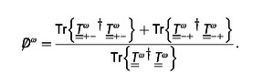
With respect to the rotationally averaged CD (CD^ω), Supp. Inf. II B contains the proof that:

$${\displaystyle {\mathrm{CD}}^{\omega }=4\pi \mathrm{Tr}\left\{{\underset{\_}{\underset{\_}{A}}}_{+}^{\omega }-{\underset{\_}{\underset{\_}{A}}}_{-}^{\omega }\right\},}$$ (10)

which, in the common units of [liter/mol/cm] reads:

$${\displaystyle {\overline{\mathrm{CD}}}^{\omega }=\frac{10N_A}{ln\left(10\right)}\frac{4\pi }{{\left(k^{\omega }\right)}^2}\mathrm{Tr}\left\{{\underset{\_}{\underset{\_}{A}}}_{+}^{\omega }-{\underset{\_}{\underset{\_}{A}}}_{-}^{\omega }\right\},}$$ (11)

where $\mathrm{Tr}\left\{\underset{\_}{\underset{\_}{F}}\right\}$ denotes the trace of the matrix $\underset{\_}{\underset{\_}{F}}$ , and N_A is Avogadro's number.

3. Exemplary Application

We now apply the T‐matrix techniques to an example based on a sodium salt of D‐camphoric acid, which is a chiral molecule. We consider a structure that is formed by four individual molecules arranged as a cross. Figure 1 shows the molecular structure.

Figure 1.

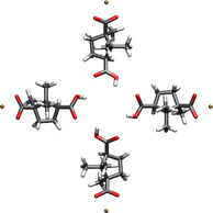
Cross‐like arrangement of four identical D‐camphoric acid chiral molecules about the origin of the coordinate system. The arrangement displays C ₄ symmetry and the center of mass of each molecule is 6.778 Å away from the origin.

The first objective is to obtain the T‐matrix of the cross. It should be noted that cross‐like structures of this particular molecule can serve as a model for the unit cell of the layers that compose some chiral SURMOFs.23 The T‐matrix of the cross is hence the main ingredient for computations of the response of the SURMOFs. Additionally, the molecular structure in Figure 1 demonstrates the applicability of our approach while the size of the system is close to the edge of what can be computed quantum mechanically as a reference.

The T‐matrix of the cross can be obtained in three steps. In a first step, we compute the single‐molecule tensors ${\underset{\_}{\underset{\_}{\alpha }}}_{pE}^{\omega }$ , ${\underset{\_}{\underset{\_}{\alpha }}}_{pH}^{\omega }$ and ${\underset{\_}{\underset{\_}{\alpha }}}_{mE}^{\omega }$ using damped response theory, also known as complex polarization propagator theory, at the TD‐HF or TD‐DFT level.24, 25 The tensor ${\underset{\_}{\underset{\_}{\alpha }}}_{pE}^{\omega }$ is the damped electric‐dipole−electric dipole linear response function and ${\underset{\_}{\underset{\_}{\alpha }}}_{pH}^{\omega }$ and ${\underset{\_}{\underset{\_}{\alpha }}}_{mE}^{\omega }$ are obtained from the damped mixed electric‐dipole−magnetic dipole linear response function. We neglect the magnetic‐dipole−magnetic dipole response ${\underset{\_}{\underset{\_}{\alpha }}}_{mH}^{\omega }$ since it is typically much smaller than the other pieces. We perform these computations in an origin‐independent way26 at the Hartree−Fock level in the def2‐TZVP basis set27 of Gaussian atomic orbitals using the turbomole program package.12, 13 The origin‐independent computation of the required tensors, described in Ref. [26] was implemented in the TURBOMOLE program package in the course of the present work. The linear response functions were obtained using sum‐over‐states expressions including the electric and magnetic transition dipoles (in the length representation) of all 29323 singlet excited TD‐HF states of the molecule. The used damping parameter corresponds to a Lorentzian line shape with full width at half maximum (FWHM) of 0.5 eV. In a second step, we use the molecular polarizabilities to build the T‐matrix of a single molecule using Eq. (6). In the third and final step, the T‐matrix of the cross‐like arrangement shown in Figure 1 is obtained using existing algorithms (see e. g. [20]). Following the customary practice of allowing higher multipolar orders in the ensemble, we set $j_{\max }=2$ . In this case, setting $j_{\max }=1$ produces essentially the same results.

As previously discussed, once the T‐matrix of the cross is available we can readily compute any kind of electromagnetic response. We focus on the average CD of the cross and investigate the accuracy and limits of the T‐matrix‐based computations.

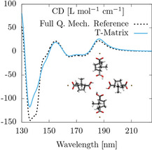
The three lines in Figures 2(a,b) show the result of the following computations. The dashed black line, labeled “Reference”, is the CD of the cross computed from 600 excitations described at the TD‐HF/def2‐TZVP level, broadened by Lorentzians with FWHM of 0.5 eV. This CD is taken as the reference result. We note the reduced number of excitations with respect to the number used for the calculation of the polarizabilities of the individual molecules. This reduction is necessary for obtaining the reference in a reasonable amount of time. The red dashed line labeled “Isolated”, and the blue continuous line labeled “Embedded” are both computed by means of the already explained three‐step procedure. Then, the CD is computed with Eq. (13). The difference between “Isolated” and “Embedded” is the initial single‐molecule TD‐HF simulation. For the “Isolated” case, the TD‐HF simulation is performed for a single molecule in vacuum. For the “Embedded” case, the TD‐HF simulation is performed for a single molecule embedded in the electrostatic potential created by the other three molecules in the cross. The potential was computed from point charges at the positions of the atomic nuclei of the three other molecules, whereby the point charges were obtained from a natural population analysis28 of the HF calculation on the cross. The potential affects the molecular orbitals and changes the intrinsic electromagnetic response of the embedded molecule. Such kind of deformation of the internal structure of a scatterer is not addressed within nor accessible by the standard T‐matrix techniques. It should be noted that such deformation is negligible in compositions of larger objects, like micro‐particles, where T‐matrix techniques are typically applied. Figures 2(a,b) show that, in the case of molecular ensembles, taking into account the embedding potential produces results that are visibly closer to the reference simulations. We stress that the difference between the overall computational complexities of the “Isolated” and the “Embedded” options is negligible: The TD‐HF calculations are far more costly than the calculation of atomic partial charges28 needed for the embedding.

Figure 2.

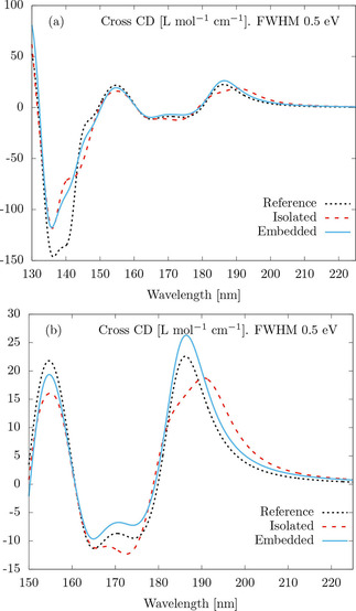
Average CD of the cross in Figure 1 as a function of the wavelength. The “Reference” black dotted lines are obtained from TD‐HF computations on the cross. The dashed red lines and solid blue lines are T‐matrix‐based calculations. For the “Isolated” case, the quantum‐mechanical single molecule simulations are performed for a molecule in vacuum. For the “Embedded” case, the molecule in vacuum is embedded in the electrostatic potential created by the three other molecules forming the cross. In both cases, the linear response damping parameter corresponds to a Lorentzian line shape with full width at half maximum of 0.5 eV. Panels (a) and (b) show two different spectral ranges. The relatively large discrepancy around 142 nm seen in panel (a) does not appear in panel (b) for a better comparison of the accuracy of the “Embedded” and “Isolated” options.

Let us discuss the results in more detail. Figure 2(a) shows that, while the three lines follow the same trends, there are some differences. The largest discrepancy occurs at the region around 142 nm, but let us first discuss the rest of the spectrum, which is shown in Figure 2(b). By comparison with the reference, we see that the “Embedded” option is superior to the “Isolated” option in terms of matching the positions, shape, and heights of the reference peaks. The electrostatically “Embedded” single molecule calculation is seemingly beneficial for the application of T‐matrix techniques in molecular ensembles. We have verified that the effect of the electrostatic deformations quickly diminishes as the separation between the four molecules forming the cross increases.

Let us now go back to the relatively large discrepancy around 142 nm that is observed for both the “Isolated” and “Embedded” options. In order to investigate it, we focus on the relevant part of the spectrum, decrease the Lorentzian FWHM from 0.5 eV to 0.025 eV, and consider larger separations for the four molecules in the cross. We consider only the “Embedded” calculations. Figure 3 shows the CD of the references (dashed lines) and the T‐matrix calculations (solid lines) for the CD of three crosses featuring different inter‐molecular distances. Namely, the labels “A”, “B”, and “C” correspond to crosses where the center‐of‐mass of the molecules is 6.778 Å (as in Figure 1), 8.400 Å and 11.646 Å away from the origin, respectively. We observe that, as the inter‐molecular distance increases: 1) The difference between the references and the T‐matrix calculations decreases, and 2) The CD spectrum quickly disappears. The latter is a clear indication that the CD bands at the region around 142 nm visible in Figure 2(a) and Figure 3 are due to aggregation. At short intermolecular distances, the four individual $\pi \to \pi {}^{*}$ excitations on the four carboxyl groups form linear combinations that transform according to the a, b, and e irreducible representations of the C ₄ point group of the cross. In the cross, the four carboxyl groups are arranged in a manner that displays axial chirality, and the a and e bands contribute to the CD spectrum at 143.1 nm and 141.9 nm, respectively (the b band is dipole forbidden). The bands are due to a purely aggregation (collective) phenomenon which explains their quick disappearance at larger intermolecular distances.

Figure 3.

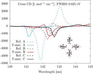
Full quantum‐mechanical “Reference” and “Embedded” T‐matrix calculations of the average CD of three different crosses. The labels “A”, “B”, and “C” correspond to crosses where the center‐of‐mass of the molecules is 6.778 Å (as in Figure 1), 8.400 Å and 11.646 Å away from the origin, respectively. The linear response damping parameter corresponds to a Lorentzian line shape with full width at half maximum of 0.025 eV.

In order to confirm this kind of aggregation phenomenon and further study the accuracy of our methodology under its presence, we study a cross built from four acetic acid molecules. Acetic acid is chosen because it features the same carboxyl group as D‐camphoric acid, but is practically achiral. Achirality of the individual molecule means that any CD observed in the cross can be unequivocally attributed to chirality that arises due to the joint arrangement, and not to the individual molecule. Moreover, as far as aggregation is concerned, the new cross should behave in a way similar to the previous one. Figure 4 shows the CD spectrum of a cross built from four acetic acid molecules. We observe strong CD bands around 142 nm. As we anticipated, this is very similar to the behavior of the cross of D‐camphoric acid molecules. The spectrum in Figure 4 is basically due to the joint axial chirality of the cross, which can be appreciated in Figure 5, where we show natural transition orbitals of the relevant electronic excitations. We again observe in Figure 4 that the T‐matrix‐based CD calculation does not predict the CD of these aggregation bands as accurately as for the case of non‐aggregation bands shown in Figure 2(b). Further research is needed to identify the origin of the discrepancy. Nevertheless, we highlight the ability of the T‐matrix technique to predict the existence of CD bands emerging due to a purely collective effect, that is, CD bands that are not present in the individual molecules.

Figure 4.

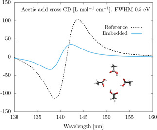
Average CD of a cross of four acetic acid molecules, with the four carboxyl groups arranged in exactly the same manner as in Figure 1. Computed at the TD‐HF/def2‐TZVP level and broadened with Lorentzians with FWHM of 0.5 eV.

Figure 5.

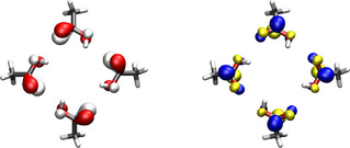
Natural transition orbitals of the cooperative $\pi \to \pi {}^{*}$ excitation responsible for the CD spectrum in the region around 142 nm. The plotted isovalue is $\pm 0.05$ $a_0^{-3/2}$ , where a ₀ is the Bohr radius. Shown are hole (red/white) and particle (blue/yellow) natural transition orbitals.

4. Prediction of Experimental Measurements

One of the prominent uses of the methodology that we introduce is the prediction of experimental electromagnetic measurements on devices of macroscopic size. As an example, we choose the computation of the total absorbance and CD of an idealized chiral SURMOF. The SURMOF model is composed of 32 planar layers. Each of the planar layers is an infinitely extended regular array whose unit cell is the molecular cross in Figure 1. The center‐to‐center distance between unit cells is $2\sqrt{2}\times 6.77$  Å. The separation between layers is 2 nm. The 64 nm thick slab lies on a substrate with a refractive index equal to 1.6.

The process of computing the response of the SURMOF goes as follows. The T‐matrix of its unit cell (the cross) is obtained, as previously discussed, from the T‐matrix of a single (“Embedded”) molecule using Lorentzians with FWHM of 0.5 eV. Then, the electromagnetic response of a single layer of crosses can be rigorously and efficiently computed with existing T‐matrix‐based algorithms, for example, with the algorithms described in Ref. [29]. The same framework allows to easily couple several identical layers stacked on top of each other, and to also include other kinds of planar layers, like slabs of homogeneous materials, which are useful for modeling substrates and microscope slides. We refer the reader to Sec. V of the Supplemental Material in Ref. [30] for details about the in‐house‐developed code that we have used.

This approach allows us to predict any kind of electromagnetic response of the SURMOF model for any illumination. As an example, we chose the total absorbance and CD under plane‐wave illumination. That is, the SURMOF is sequentially illuminated from the air side with two plane‐waves of opposite helicity (polarization handedness). Then, the total transmitted and reflected powers are measured under each illuminating handedness (±). In each case, the absorbance is computed as:

$${\displaystyle A_{\pm }=P^{\mathrm{in}}-T_{\pm }-R_{\pm },}$$ (12)

where $P^{\mathrm{in}}$ is the power of the illumination, assumed to be equal for the two different helicities, $T_{\pm }$ is the transmitted power, and $R_{\pm }$ the reflected power. We then define the total absorbance Abs and CD as:

$${\displaystyle \mathrm{Abs}=\frac{A_{+}+A_{-}}{2P^{\mathrm{in}}},\mathrm{CD}=\frac{A_{+}-A_{-}}{2P^{\mathrm{in}}}.}$$ (13)

Figure 6 shows the total absorbance and CD for two different illumination angles: $\theta =0$ , i. e. perpendicular to the plane defined by the SURMOF, and $\theta =30$ degrees. The spectral shapes of the CD lines in Figure 6 are different from those in Figure 2(b) because Figure 2(b) shows the rotationally average CD of the molecular cross, while the crosses composing the SURMOF have fixed orientations with respect to the illumination directions. We have verified this statement by simulating a very sparse single layer of crosses. The unit cell is the same, but the crosses are now spaced by 60 nm. The shapes of the CD curves of such single layer case are very similar to the ones in Figure 6.

Figure 6.

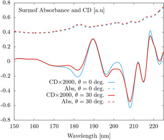
Absorbance and CD of a 32 layer SURMOF on top of a substrate under perpendicular ($\theta =0$  deg.), and oblique ($\theta =30$  deg.) illumination.

It should be noted that the response to any other incident beam, like a (focused) Gaussian beam, is readily obtained by decomposing the beam into plane‐waves and adding the respective simulation results. The computation of any other kind of measurement, like optical rotatory dispersion (ORD), can also be performed.

5. Quantification of Symmetry Breaking

The availability of T‐matrices for molecules and molecular ensembles allows to quantitatively study their symmetry‐breaking properties. Given a system and a symmetry, the question of whether the system is symmetric leads to a binary outcome, a quantification of How much does the system break the symmetry? is not possible, and the possible links between symmetry breaking and observable effects cannot be quantitatively investigated. Very recently, quantitative symmetry‐breaking measures computed from the T‐matrix have been defined.27, 28 In this section, we explain how such kind of measures open new quantitative research avenues in fundamental and technological aspects of molecular ensembles.

Molecular chirality is perhaps the most well‐know example of the symmetry‐breaking quantification problem. While the definition of when an object is chiral is simple enough, it hides significant problems that arise when attempting to measure chirality.33 It has been shown that a scalar measure of chirality allowing to rank general objects and/or to establish what a maximally chiral object is in an unambiguous way does not exist.34, 35, 36 Recently, these problems have been solved by the definition of the electromagnetic chirality (em‐chirality) of an object,31 which is based on interaction instead of geometry. It can be stated in the following way: An electromagnetically chiral object is one for which all the information obtained from experiments using a fixed incident helicity cannot be obtained using the opposite one. The electromagnetic chirality of a given object has an upper bound. In a monochromatic setting, the upper bound of the em‐chirality of an object is equal to $\sqrt{C^{\omega }}=\sqrt{\mathrm{Tr}\left\{{{\underset{\_}{\underset{\_}{T}}}^{\omega }}^{†}{\underset{\_}{\underset{\_}{T}}}^{\omega }\right\}}$ , which can be seen as a measure of how much does the object interact with the electromagnetic field. The normalized measure of em‐chirality is a number between 0 and 1 which can be computed using the singular value decomposition of the T‐matrix blocks in the helicity basis [see Eq. (8)]:

$${\displaystyle {\chi }^{\omega }=\frac{\sqrt{{∥\left[\begin{array}{c}\sigma \left({\underset{\_}{\underset{\_}{T}}}_{++}^{\omega }\right)\\ \sigma \left({\underset{\_}{\underset{\_}{T}}}_{-+}^{\omega }\right)\end{array}\right]-\left[\begin{array}{c}\sigma \left({\underset{\_}{\underset{\_}{T}}}_{--}^{\omega }\right)\\ \sigma \left({\underset{\_}{\underset{\_}{T}}}_{+-}^{\omega }\right)\end{array}\right]∥}^2}}{\sqrt{C^{\omega }}},}$$ (14)

where $\sigma \left(A\right)$ denotes the column vector of non‐increasingly‐ordered singular values of matrix A. We note that $C^{\omega }$ can also be written as

$${\displaystyle C^{\varpi }=\sigma {\left({\underset{\_}{\underset{\_}{T}}}_{++}^{\omega }\right)}^T\sigma \left({\underset{\_}{\underset{\_}{T}}}_{++}^{\omega }\right)+\sigma {\left({\underset{\_}{\underset{\_}{T}}}_{-+}^{\omega }\right)}^T\sigma \left({\underset{\_}{\underset{\_}{T}}}_{-+}^{\omega }\right)+\sigma {\left({\underset{\_}{\underset{\_}{T}}}_{+-}^{\omega }\right)}^T\sigma \left({\underset{\_}{\underset{\_}{T}}}_{+-}^{\omega }\right)+\sigma {\left({\underset{\_}{\underset{\_}{T}}}_{--}^{\omega }\right)}^T\sigma \left({\underset{\_}{\underset{\_}{T}}}_{--}^{\omega }\right),}$$ (15)

where ^T denotes transposition, which makes ${\chi }^{\omega }$ in Eq. (14) a unitless quantity.

It turns out that objects which attain the bound $\chi =1$ are transparent to all the fields of one helicity. This makes them ideal for applications like helicity dependent photon routing (see [31, Figure 4]), among others. Accordingly, achieving materials with high em‐chirality by molecular design and assembly is of great technological interest.

Furthermore, the measure of electromagnetic chirality opens up a path to tackle the quantitative understanding of how the chirality of a composite object builds up from the chirality of its components and their arrangement. Chirality is present across different spatial scales that span several orders of magnitude from high energy physics to biology, but the mechanisms by which chirality spans across spatial scales are not clear. As written in a recent review,37 “how chirality at one length scale can be translated to asymmetry at a different scale is largely not well understood”. The impossibility of comparing the chiralities of two different systems in an unambiguous way is now solved by the measure of em‐chirality, and a quantitative study of how em‐chirality is transmitted across different spatial scales becomes possible.

Another symmetry that has recently been shown to be relevant in light‐matter interactions, and in particular in chiral light‐matter interactions, is the electromagnetic duality symmetry. A system that responds in the same way to electric and magnetic fields is said to have electromagnetic duality symmetry, or, for short, to be dual. In much the same way that a translationally invariant system prevents the coupling of plane waves with different momenta during the light‐matter interaction, a dual system prevents the coupling of the two helicity components of the field, i. e. it preserves (does not mix) the two polarization handednesses. Among other phenomena,38 helicity preservation is important in optical activity. Recent work39 shows that, given a system and a pair of incident and scattered plane wave directions, the non‐mixing of the two helicities by the system is a necessary condition for optical rotation. This condition is in addition to the lack of mirror symmetry across the plane defined by the incident and scattered direction vectors. For the particular case of forward transmission through a random chiral medium like a solution of chiral molecules, the non‐mixing is achieved due to the angular momentum conservation afforded by the effective cylindrical symmetry of the random mixture. In sharp contrast, when the measurements are performed at an angle, the two relevant angular momenta do not share the same axis, there is mixing of the two helicities, and the polarization rotation angle depends on the input polarization.40 The off‐axis behavior is hence qualitatively different from the forward direction where the rotation angle is an additive constant independent of the input polarization angle. For optical activity in general incident and scattered directions, a dual system is required.41 The degree with which the optical rotation angles vary with the input polarization depends on the amount of mixing between the two helicities. Equation (2) in Ref. [41] defines a convenient measure of helicity mixing, i. e. duality breaking. The measure produces a number between 0 and 1, with 0 corresponding to perfect duality symmetry. It can be computed as:

(16)

Dual systems are also needed for other technologically important concepts like zero‐backscattering,42 metamaterials for transformation optics, Huygens wave‐front control, CD enhancing systems,30 and maximal em‐chirality since, in most cases, maximal em‐chirality implies duality symmetry. Unfortunately, naturally‐dual bulk materials do not exist, and their artificial fashioning has only been achieved at MHz frequencies.43, 44 The possibility of achieving materials with high duality by molecular design and assembly is therefore of great technological interest as well.

Going back to the cross‐like arrangement of four D‐camphoric acid molecules, Figure 7(a) shows the normalized em‐chiralities of an isolated (not electrostatically embedded) single molecule and of the cross, which are rather low in both cases. Figure 7(b) shows their duality breaking The high values of duality breaking $\approx 0.5$ are consistent with objects whose electric‐electric response ${\underset{\_}{\underset{\_}{\alpha }}}_{pE}^{\omega }$ is much larger than the magnetic‐magnetic response ${\underset{\_}{\underset{\_}{\alpha }}}_{mH}^{\omega }$ . Perfect duality symmetry at the dipolar level is met if and only if [45, Eq. (29)]: ${\underset{\_}{\underset{\_}{\alpha }}}_{pE}^{\omega }={ϵ}^{\omega }{\underset{\_}{\underset{\_}{\alpha }}}_{mH}^{\omega }$ and ${\underset{\_}{\underset{\_}{\alpha }}}_{pH}^{\omega }=-{\mu }^{\omega }{\underset{\_}{\underset{\_}{\alpha }}}_{mE}^{\omega }$ .

Figure 7.

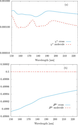
(a) Frequency dependent normalized electromagnetic chirality $\left({\chi }^{\omega }\right)$ and, (b) duality breaking of an isolated (not electrostatically‐embedded) single molecule and the cross‐like structure shown in Figure 1. Both quantities are unitless [see Eqs. (18) and (16)].

While the results in Figure 7 are far from the technologically desired ones, the examples show the usefulness of the framework put forward in this article for computing symmetry‐breaking measures of molecular ensembles.

6. Conclusions and Outlook

In conclusion, the link between quantum‐mechanical simulations and T‐matrix techniques makes it now possible to efficiently compute the electromagnetic response of molecular ensembles with very large numbers of molecules. The methodology can be used to predict the result of experimental measurements on molecular materials of macroscopic sizes. This can be applied in the analysis and molecular‐based design of discrete objects and materials for specific electromagnetic functions. We have shown that the methodology produces results which are in very good agreement with full quantum‐mechanical results, and identified further research to improve the accuracy of the predictions. We also envision new fundamental and technological research avenues related to the possibility of quantifying symmetry breaking using the T‐matrices of molecules and molecular ensembles.

Conflict of interest

The authors declare no conflict of interest.

Supporting information

As a service to our authors and readers, this journal provides supporting information supplied by the authors. Such materials are peer reviewed and may be re‐organized for online delivery, but are not copy‐edited or typeset. Technical support issues arising from supporting information (other than missing files) should be addressed to the authors.

Supplementary

I. Fernandez-Corbaton, D. Beutel, C. Rockstuhl, A. Pausch, W. Klopper, ChemPhysChem 2020, 21, 878.

References

- 1. Lieber C. M., MRS Bull. 2003, 28, 486491. [Google Scholar]
- 2. Furche F., Ahlrichs R., Wachsmann C., Weber E., Sobanski, Vögtle F., Grimme S., J. Am. Chem. Soc. 2000, 122, 1717. [Google Scholar]
- 3. Bast R., Ekstrom U., Gao B., Helgaker T., Ruud K., Thorvaldsen A. J., Phys. Chem. Chem. Phys. 2011, 13, 2627. [DOI] [PubMed] [Google Scholar]
- 4. Helgaker T., Coriani S., Jørgensen P., Kristensen K., Olsen J., Ruud K., Chem. Rev. 2012, 112, 543. [DOI] [PubMed] [Google Scholar]
- 5. Norman P., Ruud K., Saue T., Principles and Prac-tices of Molecular Properties: Theory, Modeling and Simulations, Wiley, Hoboken, NJ, 2018. [Google Scholar]
- 6. Zuehlsdorff T. J., Hine N. D. M., Payne M. C., Haynes P. D., J. Chem. Phys. 2015, 143, 204107. [DOI] [PubMed] [Google Scholar]
- 7. Seibert J., Bannwarth C., Grimme S., J. Am. Chem. Soc. 2017, 139, 11682. [DOI] [PubMed] [Google Scholar]
- 8. Waterman P. C., Proc. IEEE 1965, 53, 805. [Google Scholar]
- 9. Mishchenko M. I., Zakharova N. T., Khlebtsov N. G., Videen G., Wriedt T., J. Quant. Spectrosc. Radiat. Transfer 2016, 178, 276. [Google Scholar]
- 10. Egel A., Pattelli L., Mazzamuto G., Wiersma D. S., Lemmer U., J. Quant. Spectrosc. Radiat. Transfer 2017, 199, 103. [Google Scholar]
- 11. Jackson J. D., Classical Electrodynamics, Wiley, New York City, 1998. [Google Scholar]
- 12. Furche F., Ahlrichs R., Hättig C., Klopper W., Sierka M., Weigend F., WIREs Comput. Mol. Sci. 2014, 4, 91. [Google Scholar]
- 13.TURBOMOLE V7.2 2017, a development of University of Karlsruhe and Forschungszentrum Karlsruhe GmbH, 1989–2007, TURBOMOLE GmbH, since 2007; available from http://www.turbomole.com.
- 14. Autschbach J., Chirality 2009, 21, E116. [DOI] [PubMed] [Google Scholar]
- 15. Sersic I., Tuambilangana C., Kampfrath T., Koenderink A. F., Phys. Rev. B 2011, 83, 245102. [Google Scholar]
- 16.M. S. Wheeler, A scattering-based approach to the design, analysis, and experimental verification of magnetic meta- materials made from dielectrics, Ph.D. thesis, University of Toronto (2010).
- 17. Fernandez-Corbaton I., Nanz S., Alaee R., Rockstuhl C., Opt. Express 2015, 23, 33044. [DOI] [PubMed] [Google Scholar]
- 18. Alaee R., Rockstuhl C., Fernandez-Corbaton I., Opt. Commun. 2018, 407, 17. [Google Scholar]
- 19. Alaee R., Rockstuhl C., Fernandez-Corbaton I., Adv. Opt. Mater. 2019, 7, 1800783. [Google Scholar]
- 20. Mishchenko M. I., Travis L. D., Mackowski D. W., J. Quant. Spectrosc. Radiat. Transfer 1996, 55, 535. [Google Scholar]
- 21. Xu Y.-L., J. Opt. Soc. Am. A 2013, 30, 1053. [DOI] [PubMed] [Google Scholar]
- 22. Xu Y.-L., J. Opt. Soc. Am. A 2014, 31, 322. [Google Scholar]
- 23. Gu Z.-G., Brck J., Bihlmeier A., Liu J., Shekhah O., Weidler P. G., Azucena C., Wang Z., Heissler S., Gliemann H., Klopper W., Ulrich A. S., Wöll C., Chem. Eur. J. 2014, 20, 9879. [DOI] [PubMed] [Google Scholar]
- 24. Jiemchooroj A., Norman P., J. Chem. Phys. 2005, 126, 134102. [DOI] [PubMed] [Google Scholar]
- 25. Cukras J., Kauczor J., Norman P., Rizzo A., Rikken G. L. J. A., Coriani S., Phys. Chem. Chem. Phys. 2016, 18, 13267. [DOI] [PubMed] [Google Scholar]
- 26. Autschbach J., ChemPhysChem 2011, 12, 3224. [DOI] [PubMed] [Google Scholar]
- 27. Weigend F., Ahlrichs R., Phys. Chem. Chem. Phys. 2005, 7, 3297. [DOI] [PubMed] [Google Scholar]
- 28. Reed A. E., Weinstock R. B., Weinhold F., J. Chem. Phys. 1985, 83, 735. [Google Scholar]
- 29. Stefanou N., Yannopapas V., Modinos A., Comput. Phys. Commun. 2000, 132, 189. [Google Scholar]
- 30. Feis J., Beutel D., K“opfler J., Garcia-Santiago X., Rockstuhl C., Wegener M., Fernandez-Corbaton I., Phys. Rev. Lett. 2020, 124, 033201. [DOI] [PubMed] [Google Scholar]
- 31. Fernandez-Corbaton I., Fruhnert M., Rockstuhl C., Phys. Rev. X 2016, 6, 031013. [Google Scholar]
- 32. Fernandez-Corbaton I., J. Phys. Commun. 2018, 2, 095002. [Google Scholar]
- 33. Fowler P. W., Symmetry: Culture and Science 2005, 16, 321. [Google Scholar]
- 34. Buda A. B., Mislow K., J. Am. Chem. Soc. 1992, 114, 6006. [Google Scholar]
- 35. Petitjean M., Entropy 2003, 5, 271. [Google Scholar]
- 36. Rassat A., Fowler P. W., Chem. Eur. J. 2004, 10, 6575. [DOI] [PubMed] [Google Scholar]
- 37. Morrow S. M., Bissette A. J., Fletcher S. P., Nat. Nanotechnol. 2017, 12, 410. [DOI] [PubMed] [Google Scholar]
- 38.I. Fernandez-Corbaton, Helicity and duality symmetry in light matter interactions: Theory and applications, Ph.D. thesis, Macquarie University (2014), arXiv: 1407.4432.
- 39. Fernandez-Corbaton I., Vidal X., Tischler N., Molina-Terriza G., J. Chem. Phys. 2013, 138, 214311. [DOI] [PubMed] [Google Scholar]
- 40. Vidal X., Fernandez-Corbaton I., Barbara A. F., Molina-Terriza G., Appl. Phys. Lett. 2015, 107, 211107. [Google Scholar]
- 41. Fernandez-Corbaton I., Fruhnert M., Rockstuhl C., ACS Photonics 2015, 2, 376. [Google Scholar]
- 42. Slivina E., Abass A., Bätzner D., Strahm B., Rockstuhl C., Fernandez-Corbaton I., Phys. Rev. Appl. 2019, 12, 054003. [Google Scholar]
- 43.L. Sengupta, S. Sengupta, “Composites of magnesium ferrite materials combined with ferroelectric ceramic barium strontium titanium oxide; adjustable dielectric and magnetic properties,” (2000), US Patent 6,063,719.
- 44.N. Schubring, J. Mantese, A. Micheli, “Ferroelectric and ferromagnetic material having improved impedance matching,” (2004), US Patent 6,689,287.
- 45. Fernandez-Corbaton I., Molina-Terriza G., Phys. Rev. B 2013, 88, 085111. [Google Scholar]
Associated Data
This section collects any data citations, data availability statements, or supplementary materials included in this article.
Supplementary Materials