Quantitative Proteomics of the Cancer Cell Line Encyclopedia

Summary

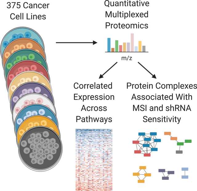
Proteins are essential agents of biological processes. To date, large-scale profiling of cell line collections including the Cancer Cell Line Encyclopedia (CCLE) has focused primarily on genetic information while deep interrogation of the proteome has remained out of reach. Here we expand the CCLE through quantitative profiling of thousands of proteins by mass spectrometry across 375 cell lines from diverse lineages to reveal information undiscovered by DNA and RNA methods. We observe unexpected correlations within and between pathways that are largely absent from RNA. An analysis of microsatellite instable (MSI) cell lines reveals the dysregulation of specific protein complexes associated with surveillance of mutation and translation. These and other protein complexes were associated with sensitivity to knockdown of several different genes. These data in conjunction with the wider CCLE are a broad resource to explore cellular behavior and facilitate cancer research.

Graphical abstract

Introduction

Proteins are the executors of the function encoded by a cell’s genome. Although commonly used as a proxy for protein expression, on average RNA expression data predict protein expression poorly (Gygi et al., 1999; Liu et al., 2016). Unfortunately generation of high quality proteomics data has lagged behind RNA expression profiling. Recently, proteomic studies of several cancers have rediscovered many of the same subtypes found by gene expression, as well as new disease categorizations, highlighting the gains from studying the proteome (Mertins et al., 2016; Pozniak et al., 2016; Zhang et al., 2014, 2016; Vasaikar et al., 2019).

The posttranscriptional mechanisms underlying the differences between protein and RNA expression are well enumerated. However, despite significant mechanistic understanding, there is less clarity about the global organization of gene and protein expression and where they differ. Correlated expression patterns in gene expression data are organized in large part around chromosomal location, driven by mechanisms such as transcription factor activity and chromosomal topology as set up by cellular and tissue identity (Caron et al., 2001; Dixon et al., 2016; Furlong and Levine, 2018; Hnisz et al., 2017). These patterns are reduced or absent in protein expression data (Grabowski et al., 2018; Kustatscher et al., 2017), leading to a model where posttranscriptional events buffer gene expression changes to create a new pattern of protein abundance. The degree to which this occurs is unclear and likely dependent on individual genes and the biological phenomena at play (Jovanovic et al., 2015; Liu et al., 2016). In contrast to RNA expression, protein expression is organized by protein interactions and subcellular localization (Dephoure et al., 2014; Gonҫalves et al., 2017; Kustatscher et al., 2017; Lapek et al., 2017; Pozniak et al., 2016; Roumeliotis et al., 2017). Although these findings have appeared consistently, the extent to which they contribute to the organization of the proteome and if other organizing principles are at work are unknown.

Cancer cell lines are important model systems to study normal and aberrant cellular processes. The Cancer Cell Line Encyclopedia (CCLE) is an effort to generate large-scale profiling data sets across nearly 1,000 cell lines from diverse tissue lineages. Its original release included gene expression, DNA copy numbers, and hybrid capture sequencing (Barretina et al., 2012). Recently, histone profiling, RNASeq, DNA methylation, miRNA profiling, and whole genome sequencing, and metabolite profiling were added (Ghandi et al., 2019; Li et al., 2019). Associated drug and shRNA sensitivity screens increased the richness of data attached to the CCLE (Basu et al., 2013; Meyers et al., 2017; Tsherniak et al., 2017). With its latest release, the CCLE includes targeted protein quantification by reverse-phase protein arrays, but deep proteome profiling is absent (Ghandi et al., 2019). Although cell lines are popular models (Frejno et al., 2017; Gholami et al., 2013), no large-scale proteomics study of human samples across a diverse population as in the CCLE has been performed.

Cancer arises from mutation, but the character of that mutation differs between cancers (Lawrence et al., 2013). A subset of cancers, hypermutated/microsatellite instable (MSI) colorectal cancers, possess orders of magnitude more mutations than other tumors (Campbell et al., 2017; Lawrence et al., 2013; The Cancer Genome Atlas Network, 2012). How a cancer proteome adapts to the negative selective effects of an extremely high mutation burden is unknown. Additionally, these tumors have increased levels of neoantigens making them attractive for immunooncology therapies (Baretti and Le, 2018). MSI is the dominant form of hypermutation present in the CCLE and while the MSI proteome has been studied in colorectal cell lines and tumors (Halvey et al., 2013; Liu and Zhang, 2016) it has not been explored across tissue lineages.

Here we have profiled 375 cell lines in the CCLE by mass spectrometry. All of the data are available at https://gygi.med.harvard.edu/publications/ccle and https://depmap.org. We find that the primary variation in protein expression appears to be organized around biological pathways, with unexpected correlations between members of entirely different pathways. We leverage the data to better understand the effects of MSI on the proteome, finding substantial buffering of transcriptional effects. Exploring the relationship between genetics and protein complex levels uncovered associations between protein complexes and sensitivity to gene knockdown and mutation. The addition of quantitative proteomics to the CCLE presents opportunities to understand the proteome in conjunction with the many other data sets present in the CCLE to improve our understanding of cancer and basic cellular biology.

Results

We selected 375 cell lines from the CCLE for quantitative protein expression profiling (Tables SI and S2). The cell lines were distributed among 22 lineages, dominated by solid organs (Fig. 1A). The experiment used sample multiplexing by TMT10-plex reagents and the best available instrumentation. These technologies enabled good depth of coverage with a high degree of overlap between samples and uncompromised quantitation. At a 1% protein-level FDR over 12,000 proteins were quantified among all samples, and over 9,000 in a majority of samples (Fig. 1B and SIC). Representation of categories was as expected, with good coverage of abundant proteins like the ribosome and incomplete coverage of lower abundance ones like transcription factors (Fig. SID). The first two batches of 9 samples were each prepared in biological triplicate, with the latter two replicates grown one year later (Table S3). In all cases, triplicates clustered together with the latter two replicates clustered more tightly (Fig. 1C). The average correlation between replicate samples was 0.8 and between different cell lines was −0.05 (p < 2e-16), with a median CV of 60% between biological replicate protein measurements within a cell line. There was visible, though incomplete, clustering by tissue lineage (Fig. 1C and 2A). Protein expression among samples was highly variable but generally consistent with previous data. For example, ERBB2 (HER2) is upregulated in a breast-derived line in the replicate dataset (Fig. 1D). In the complete dataset the pattern is complex, but ERBB2 is upregulated in several breast lines and is largely predicted by ERBB2 copy number (Fig. 1E). Among the non-breast lines with the highest levels were many with already-reported high expression levels (Ise et al., 2011; Kim et al., 2008; Mimura et al., 2005; Scott et al., 1993).

Figure 1. Quantitative Proteomic analysis of 375 diverse cancer cell lines.

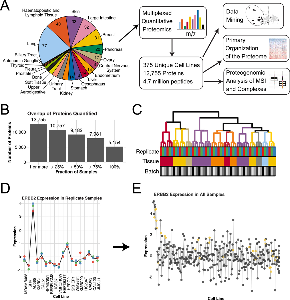
(A) Overview of the data set and analyses conducted. (B) Overlap of proteins quantified across all samples. (C) Clustering of biological replicates (n=3) for the first 18 cell lines. Tissues are colored as in panel A. (D) ERBB2 (HER2) protein expression in the biological replicate set shows high levels in a single breast cancer line. Colored dots show individual replicates and the line is the mean. (E) ERBB2 protein expression across the full data set. Cell lines are arranged along the x-axis by ERBB2 copy number. Cell lines with increased copy number (left) have high levels of ERBB2 and are frequently breast derived (yellow). See also Tables S1-3.

Figure 2. Correlation between protein and RNA expression.

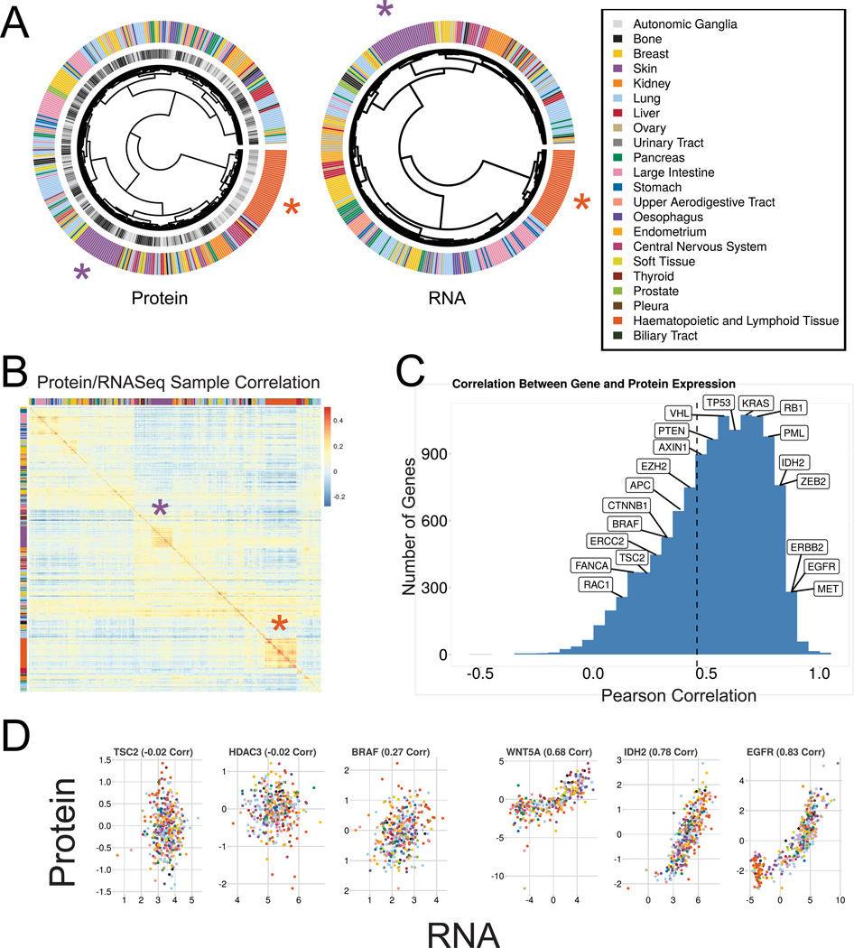
(A) Hierarchical clustering using proteins quantified in all samples (left) and their corresponding RNASeq expression (middle). (B) Correlation between samples for protein expression (y-axis) and RNASeq (x-axis). In all cases the most highly correlated RNASeq sample to any given protein sample was the same cell line. Clusters of similarity for lymphoid lines and skin lines are highlighted in A-B with orange and purple asterisks respectively. (C) Per-gene Pearson correlation between protein and RNA expression for all proteins quantified. Mean correlation is 0.48 (dashed line). The locations of several cancer-related genes are shown. (D) Examples of the RNA and protein expression for both low (left) and high (right) correlating genes. See also Table S4.

Hierarchical clustering had some coherency based on tissue lineage (Fig. 2A left). We quantified this using Gini purity, a measure of clustering specificity. Our clustering had a mean Gini purity of 0.46 where 1.0 would be perfect clustering by lineage. Clustering of the RNA data had similarly complex clustering (Fig. 2A center). In both cases, skin and haematopoetic/lymphoid lineages clustered more tightly with themselves than other lineages (Fig. 2A-B, purple and orange asterisks respectively) which differed substantially from the clusters recently reported from RPPA data (Li et al., 2017). Although the protein data had slightly less lineage coherency than RNA (mean Gini purity of 0.6 in the RNA) both showed incomplete clustering. Examining the correlation of protein and RNA expression by sample, in all cases the protein data were most highly correlated with the corresponding RNA data from the same cell line, providing additional confidence in our results (Fig. 2B).

The diversity and depth of these data allowed us calculate the RNA/Protein correlation of individual genes. Here, the correlations between RNA and protein expression varied widely, averaging at just under 0.5, in line with previous studies (Fig. 1 C-D, Table S4) (Edfors et al., 2016; Roumeliotis et al., 2017; Zhang et al., 2014). For some genes RNA expression was a good proxy for protein levels (e.g. EGFR) where for others it provided little information (e.g. BRAF) (Fig. 2D).

We examined the consistency of high or low correlations between RNA and protein levels using Gene Set Enrichment Analysis (GSEA, Subramanian et al., 2005) (Table S4). Hundreds of pathways and GO categories had higher or lower than expected protein/RNA correlations. Those with the consistently highest correlations were epithelial mesenchymal transition and various cell surface protein-related pathways associated with the epithelia. Among those with the consistently lowest correlations were gene sets with notable protein complexes. Several dozen transcription factors showed sets of targets with high RNA/protein correlation, and none with consistently low correlation.

Correlated Biological Pathways and Processes Organize a Significant Amount of Protein Expression

The results of hierarchical clustering in Figure 2A were reflected in the PCA projection of the same data. There, the haematopoetic and lymphoid lineages segregated from the solid organ lineages, making up a large part of the PC1 projection (Fig. 3A). By themselves, the haematopoetic and lymphoid lines separated by PCA (Fig. S2A). Thus, these cell lines are significantly different from both the solid organ-derived lineages and from each other. Following previous work (Barretina et al., 2012), we therefore removed the haematopoetic and lymphoid lines from further analyses.

Figure 3. The primary variation in protein expression for most cell lines is organized by coordinated expression of protein complexes and cellular pathways.

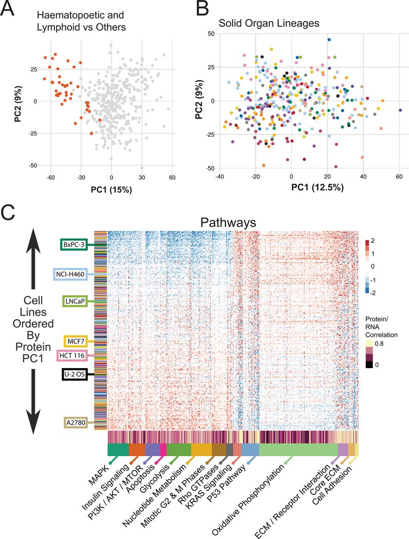
(A) PCA of the protein expression data for all samples. Dark orange points are haematopoetic and lymphoid lineages. (B) PCA projection after removing haematopoetic-and lymphoid-derived lines. (C) Heatmap of coordinated expression levels of example pathways. The x-axis is individual proteins belonging to the annotated complex or pathway. The y-axis is the cell lines rank ordered by the PC1 projection (x-axis in panel B). The Pearson correlation between protein and RNA expression for each individual gene is annotated along the x-axis. Examples of commonly used cell lines are annotated. Colors in B and y-axis of C are lineages as in Figure 1A. See also Table S5.

The remaining lines showed a complex PCA projection, with overlapping tissue lineages, particularly along PC1 (Fig. 3B). Subsequent principal components had strong tissue effects as expected, but PC1 could not be understood based on tissue. However, the underlying biology affects a large fraction of the total proteome, as 75% of all proteins had expression levels that were significantly correlated with the cell line’s PC1 projection at a 1% FDR.

We also attempted to explain the PC1 organization based on mutation. Although differences in total mutational burden are a hallmark of different tumor types (Lawrence et al., 2013) this explanation did not apply (Fig. S2C). We also attempted to computationally select a group of mutations that would predict the PC1 projection (Fig. S2D).

While some mutations were correlated with one or the other ends of the PC1 projection, the effect was incomplete and usually tied to a given tissue. From these results it appears that mutation, like tissue lineage, is not the dominant organizer of the coordinated proteome organization accounting for PC1.

Protein complex membership has been described as the major driver of proteome covariation with some lesser contribution by pathway membership (Romanov et al., 2019) but how the covarying expression of these organizing units might affect our results was not clear. We hypothesized that the PC1 projection might result from organized protein co-expression due to shared biological function instead of tissue lineage or mutation. To test this we used GSEA on the protein loadings for PC1 (Fig. 3–4). We observed over 200 pathways enriched across the PC1 loadings (Fig. 3C and 4B, Table S7). This enrichment was a result of correlated expression of a subset of pathway members, examples of which are shown in Figures 3C and 4A. These can be grouped broadly as large protein complexes and gene sets with more transient or absent protein-protein interactions.

Figure 4. Coordinated expression across biological processes is associated with the major variation in the cellular proteome.

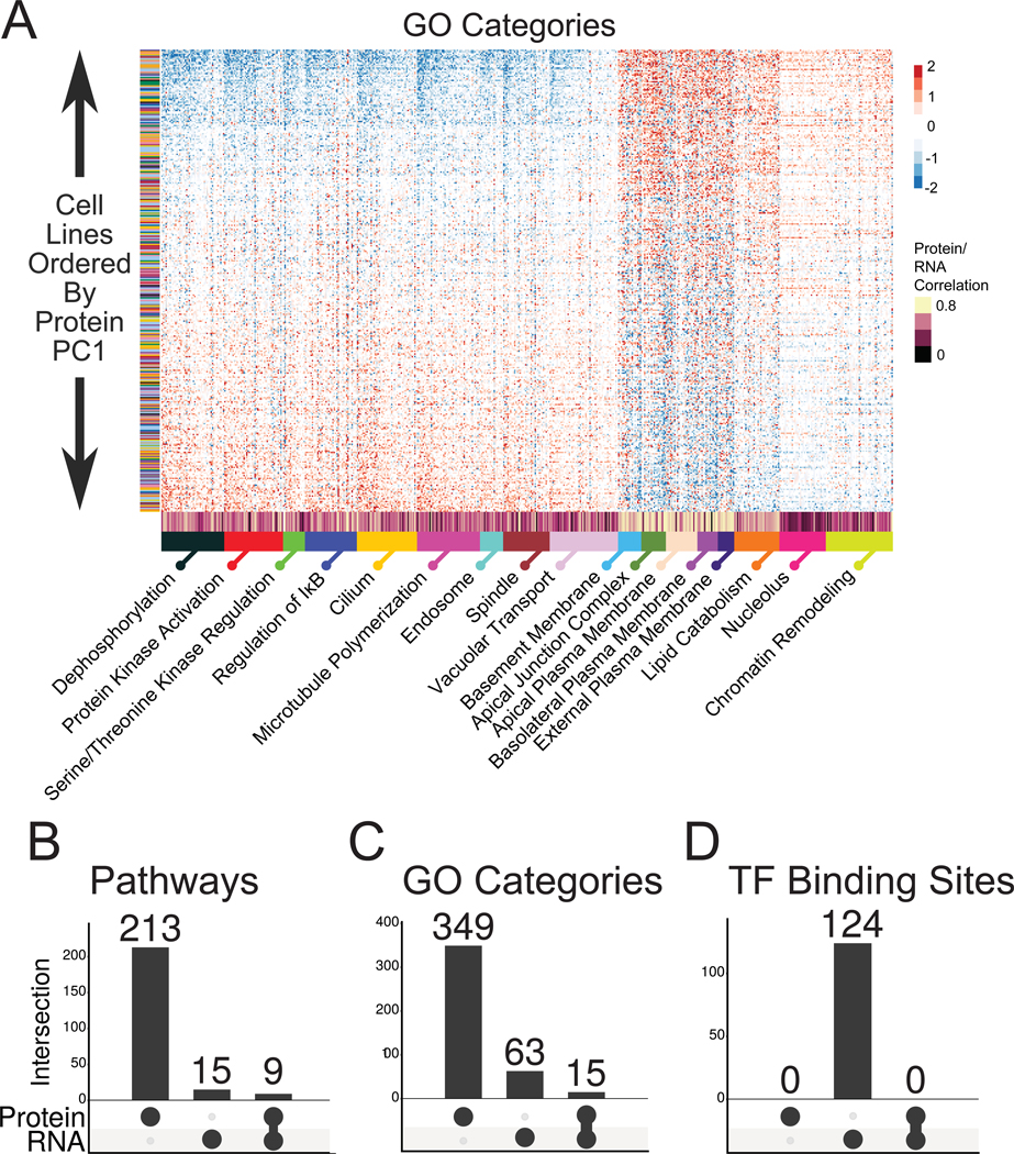
(A) Selected GO categories enriched in the PC1 loadings. As in Figure 3C, cell lines are arranged in rank order according to PC1 projection. (B-D) GSEA on the PC1 loadings for both protein expression and RNASeq data were performed separately using (B) pathway (C) GO and (D) transcription factor binding site databases. The number of enriched gene sets for each is shown as is the overlap between the protein and RNA.

The non-protein complex gene sets (Fig. 3C) encompassed features including growth factor signaling, metabolism, and epithelial phenotype. Cell lines distributed along the PC1 projection fell along one of two anticorrelated patterns of protein expression composed of members of many different pathways. One pattern included upregulation of members of growth factor signaling pathways including MAPK and insulin receptor signaling, metabolic pathways including glycolysis and nucleotide metabolism, and cell division. The other pattern included upregulated cell-cell and cell-matrix adhesion pathways that are hallmarks of epithelia, KRAS and p53 signaling markers, and oxidative phosphorylation. Strikingly, the glycolysis pathway was anticorrelated with the oxidative phosphorylation pathway. The switch between these pathways is characteristic of the Warburg effect, a phenotype of cancer similarly fundamental as epithelial and mesenchymal phenotype. The relative expression levels of these pathway proteins are largely disconnected from tissue lineage (Fig. 3C, y-axis). Performing the same analysis using GO categories found hundreds more gene sets with enriched coexpression (Fig. 4A, C, Table S7).

The remaining gene sets were defined by large protein complexes (Fig. S2B). These complexes were included in many pathways not primarily associated with them, and as a result were found as significantly enriched almost entirely because of their presence in the gene set (Table S7). These complexes showed highly correlated coexpression despite low total variation across the samples, consistent with their housekeeping roles, and demonstrating that their levels are tightly controlled.

RNA Expression Does Not Capture the Primary Organizing Variation of the Steady State Proteome

We expected that RNA data would capture much of the pathway-level correlations observed in the protein data. However, when we performed a PCA projection on the RNA data for the same cell lines followed by GSEA on its PC1 loadings, as we had done on the protein data, far fewer pathways and GO categories were enriched along the RNA PC1, some of which overlapped with the protein data (Fig. 4 B-C and Table S7).

To visualize these results we annotated the per-gene correlations between RNA and protein levels on the heatmaps in Figures 3–4 and S2. Protein complexes exhibited very low overall correlation with RNA levels, in line with previous results (Fig. S2B and Table S7). The pathway results varied, with most pathways in Figure 3C having average correlations. However, a handful of pathways in Figure 3C had very high correlation with RNA expression, most notably cell surface proteins that mediate cell contact, as well as KRAS and p53 signaling markers (Table S7). A similar result was found for the GO categories in Figure 4A. These gene sets also displayed more extreme changes across PC1, whereas the proteins with a lower correlation to RNA had a more subdued gradient.

These results did not explain the underlying organization of the RNA expression data and how it differed from protein expression. One model is that transcriptional mechanisms are the primary organizers of RNA levels, and that subsequent mechanisms refine protein expression levels to create the broad patterns of co-expression observed in Figures 3C and 4A. To examine this, we performed the same analysis using GSEA on PC1 loadings for the protein and RNA data using a transcription factor binding target database. This resulted in over a hundred transcription factor target enrichments in the RNA data and none in the protein data (Fig. 4D and S2E). Surprisingly, the same gradient of expression found in the RNA data in Figure S2E was visible in the protein expression levels, albeit more weakly. Thus, it appears that while RNA levels carry through into protein levels, they are not the organizer of the primary component of variation of the steady state proteome.

A Large Fraction of the Proteome is Correlated With Epithelial and Mesenchymal Markers

In solid organ tumors, the epithelial and mesenchymal states affect progression, malignancy, and resistance to treatment (Ye and Weinberg). These fundamental states are associated with large changes in gene and protein expression resulting in histologically visible differences, however to what extent has not been described for the proteome. Because the broad alignment of pathways in the PC1 projection appeared to correlate with known epithelial markers we correlated the expression of all proteins to EPCAM and VIM, the canonical epithelial and mesenchymal markers that were among the most anticorrelated proteins in the expression correlation network described below. EPCAM was the protein with the highest loading in PC1, and VIM was in the 50 most negative loadings, making them examplars of the general trends across cell lines. Nearly half of all proteins were positively or negatively correlated with EPCAM expression (Fig S3A) and about a third of all proteins were positively or negatively correlated with VIM expression (Fig S3B). In both cases, about half of the correlated proteins also had mRNA expression that correlated with these markers, and a substantial fraction of the mRNAs that showed correlation with these markers did not show a corresponding protein-level correlation. In total, these results present the epithelial and mesenchymal states as the product of controlled expression of much of the genome, with significant posttranscriptional regulation to shape the levels of between approximately 1/3 to half of all expressed proteins in solid organ lineages.

Cell Line Sensitivity is Correlated With Broad Proteome Coexpression

The projection of each cell line along PC1 approximates the many pathways shown in Figures 3–4. We hypothesized that this higher level state could predict sensitivities to gene disruptions and drug treatments. To test this, we correlated the PC1 projection of each cell line with its associated sensitivity scores in CRISPR screening (Fig. S4A-B) or drug treatment (Fig. S4C-D). Several dozen genes in a CRISPR screen showed correlated sensitivities including well known genes associated with cancer such as PIK3CB and ZEB2 (Fig. S4A-B). There was a significant enrichment of genes that encode cell surface proteins in this set, most notably several integrins (Fig. S4A bolded text and S4B).

Several drugs also had effects correlated with cell line PC1 projection (Fig. S4C-D). The largest subset is EGFR-targeting drugs (Fig. S4C, green text) but also those targeting other proteins including PIK3CB and EIF4. We conclude that the broad-scale coordinated expression of members of many pathways at the proteome level is correlated with several drug and gene loss sensitivities.

An Expression Correlation Network Captures Associations Between Proteins

Expression correlation networks have been useful for organizing and exploring large-scale protein expression data (Lapek et al., 2017; Pozniak et al., 2016; Roumeliotis et al., 2017). We constructed a correlation network from our data in solid organ-derived lineages, containing of 3,777 proteins and 41,600 correlations at an estimated 1% FDR, of which nearly 40,000 were positive correlations (Fig S5A, Table S6).

Because many different mechanisms can affect protein levels, we sought to annotate the network with putative shared mechanisms that might be responsible for correlated expression between any two proteins. The most obvious mechanism determining protein co-expression is gene co-expression. To assess this we built a correlation network using the CCLE RNASeq data and looked for shared edges with the protein network. The RNA network was far denser, containing over 195,000 correlations between ~9,400 genes. Nearly 5,500 edges in the protein correlation network were shared with RNA (Fig. S5B-C). The most notable cluster of these was the anticorrelation between EPCAM and VIM (Fig. S5D), each of which was positively correlated with proteins related to epithelial and mesenchymal function.

We also examined protein-protein interaction databases, finding over 6,300 edges could be annotated by protein-protein interactions and shared complex membership. Many well-studied complexes (Fig. S5E) were shared between these data types, all of which were composed of positive expression correlations. Several complexes shared edges with correlation networks built from CRISPR (Meyers et al., 2017) and shRNA sensitivity data (McDonald et al., 2017), similar to recent work (Pan et al., 2018). Shared localization between correlated proteins also provided annotations for about 3,500 edges.

The largest number of protein expression correlations that we could annotate came from shared pathway membership. Over 7,900 network edges, half the total annotated, were between proteins from the same pathway. While some of this set is potentially explained by shared gene expression or complex membership a very large portion were not (Fig. S5B-C).

Multiple Protein Complexes Are Differentially Expressed in Microsatellite Instable Cell Lines

We sought to investigate the effect of high mutation burden on the proteome. MSI is by far the dominant form of hypermutation in the CCLE. Although the proteome of MSI colorectal cancer has been analyzed recently in a panel of ten cell lines and in the TCGA tumor data (Halvey et al., 2013; Liu and Zhang, 2016; Zhang et al., 2014), the CCLE contained MSI samples of multiple tissue lineages. The mRNA data had over a thousand significantly up-and downregulated genes associated with MSI (Fig. 5A). However, in a stark contrast the protein expression data only showed a total of 50 proteins with altered expression in MSI cells, 30 of which were shared with the mRNA data. Among these 50 proteins was an obvious enrichment of multiple protein complexes that monitor DNA, RNA, and nascent proteins for mutation or problems in translation (Fig. 5B-C).

Figure 5. Microsatellite Instability is associated with downregulation of multiple protein complexes.

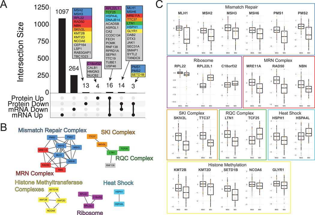
(A) Overlap of significantly up-and downregulated mRNA and protein levels associated with MSI status. (B) High confidence protein associations taken from the STRING database are plotted as a network and colored according to complex membership. Only connected nodes are shown. (C) Expression levels (y-axis) of proteins in Microsatellite Stable (MSS, left) and MSI (right) for the complex members shown in panel B. Boxplots are standard, showing the median at the horizontal line, first and third quartiles at the hinges, and the whiskers at the most extreme values no further than 1.5 times the interquartile range beyond the hinge.

Many proteins with well-established ties to MSI were recovered. As expected, members of the mismatch repair complex were downregulated (Figure 5A-C). Loss of function of this complex can cause hypermutation in colorectal cancer (Eshleman and Markowitz, 1996; The Cancer Genome Atlas Network, 2012). Other complexes that were downregulated with at least one member that was previously associated with MSI included the MRN complex (Dorard et al., 2011; Giannini et al., 2004; Halvey et al., 2013), and the ribosomal accessory proteins RPL22 and RPL22L1 (Chan et al., 2019; Ghandi et al., 2019; McDonald et al., 2017) (Fig. 5). In addition, two categories of proteins with one member previously associated with MSI were downregulated in MSI cells. The heat shock proteins HSPA4L, DNAJB14, and HSPH1 (aka HSP110) were also downregulated in MSI, the latter of which has an established role in MSI disease (Causse et al., 2019; Dorard et al., 2011). The histone methyltransferase (HMT) proteins KMT2B, KMT2D, and SETD1B were also downregulated in MSI cells, with SETD1B previously associated with MSI colorectal and gastric cancer (Choi et al., 2014).

Two ribosome-associated protein complexes were unexpectedly differentially regulated in MSI. The SKI complex is a cytoplasmic ribosome-associated protein complex that performs RNA monitoring, moving problematic mRNAs from the ribosome to the exosome for degradation (Halbach et al., 2013; Schmidt et al., 2016). Its helicase component (SKIV2L) and an associated binding partner (TTC37) are both downregulated in MSI cell lines (Fig. 5A). The Ribosomal Quality Control (RQC) complex surveys newly synthesized proteins exiting the ribosome (Brandman et al., 2012). LTN1 is a ubiquitin E3 ligase member of the RQC that specifically targets dysfunctional nascent proteins for degradation by the proteasome. LTN1 was expressed at lower levels in MSI lines, while its putative co-complex member TCF25 was upregulated. All together, the members of these various protein complexes represent 24 out of 50 total significantly altered proteins in MSI.

MSI-Associated Proteins Differentially Correlate With the MutL and MutS Complex Expression

Although the relationships between members of the same complex was clear, how the different complexes were related was unknown. Correlating the expression patterns in MSI lines of the proteins found in all samples revealed multiple clusters (Fig. 6A). As expected, proteins within the same complex clustered together. However, the top level hierarchical split separated the mismatch repair constituent complexes, MutL and MutS, and with them the other complexes identified (Fig. 6A). The HMT complex proteins were present in the cluster containing MutL. In contrast, the MRN and SKI complexes as well as LTN1 clustered with the MutS complexes (Fig. 6A). These correlated relationships between complexes were very different in non-MSI lines (Fig. 6B).

Figure 6. Associations between protein complexes altered in MSI cell lines.

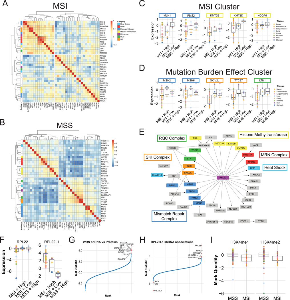
(A-B) Heatmaps of the correlation matrix between all proteins altered in MSI cell lines that were quantified in all samples. Correlations are for protein expression levels in MSI (A) and MSS lines (B). (C-D) Protein complex members are differentially expressed according to a combination of MSI status and total mutation burden. Some proteins are associated with MSI alone (C) or a combination of MSI and total mutation burden (D). (E) Significant associations between mutated genes (arrow base) and protein expression levels (arrowheads) are plotted as a network. RPL22 mutation is significantly associated with expression changes in the same protein complex members as are altered in MSI. (F) RPL22 and RPL22L1 expression levels as in (C-D). (G-H) Protein expression associations with sensitivity to shRNA knockdown of WRN (G) and RPL22L1 (H). Proteins are ranked along the x-axis by their linear model test statistic and arranged according to that test statistic along the y-axis. Significantly associated proteins are shown in red and labeled. (I) H3K4me1 and me2 levels in MSS and MSI cell lines. Boxplots are as in Figure 5.

MSI is one form of hypermutation, although other causes of hypermutation exist including exposure to mutagens like UV light and cigarette smoke as well as APOBEC activity. The hypermutated samples in the CCLE are dominated by MSI, but several non-MSI hypermutated lines are present and bear the signatures of one or several of these other causes (Ghandi et al., 2019). To investigate if MSI, mutation burden or a combination was responsible for the above clustering, we compared three linear models for each protein’s expression: one using MSI status, one using total mutation burden, and one using an interaction between MSI status and mutation burden. The set of proteins whose expression correlated with MutL were generally best fit by a model using MSI status alone (Fig. 6C). This included the MutL components MLH1 and PMS2, and HMT complex members. In the cluster that included MutS, SKIV2L, TTC37, and LTN1, accounting for mutation burden generally improved the model fit over MSI status alone (Fig. 6D).

RPL22 Mutation Is Uniquely Associated With Protein Complexes Differentially Expressed in MSI

In a parallel analysis we examined the effect of mutations in individual genes on protein expression levels across all solid organ derived cell lines. We observed hundreds of associations between gene mutations and protein levels (Fig. S6, Table S7). KRAS mutation had significant associations with the levels of many proteins (Fig. S6A) most of which were associated with cell motility and adhesion. TP53 mutation had a handful of associated proteins, most of which were members of the p53 pathway or other DNA damage response proteins (Fig S6B).

This analysis highlighted RPL22 as it was obviously uniquely associated with protein expression changes in complexes like mismatch repair (Fig. 6E). RPL22 was identified as a mutation hotspot in MSI endometrial cancers (Novetsky et al., 2013). Upon RPL22 loss RPL22L1 expression is derepressed and provides a functional substitution (McDonald et al., 2017; O’Leary et al., 2013). RPL22 was identified as an interactor with MDM2 that suppresses p53 degradation (Cao et al., 2017). The second-generation analysis of the CCLE found a relationship between MDM4 splicing and RPL22L1 levels, in line with the relationship between RPL22 and p53 (Ghandi et al., 2019). Recently, RPL22L1 sensitivity was identified in the DRIVE data as a strong hit for sensitivities in MSI cell lines (Chan et al., 2019). Despite this prior work the role of RPL22/RPL22L1 in mismatch repair deficient cancer is unclear.

RPL22 expression in MSI cells clustered with the MutS complex (Fig. 6A), and the best model fit for both RPL22 and RPL22L1 was the combination of MSI and mutation burden (Fig. 6F), as with the SKI complex and LTN1. Multiple groups recently reported that MSI cells are sensitive to WRN loss (Behan et al., 2019; Chan et al., 2019; Lieb et al., 2019). Analysis of the DRIVE data revealed that the protein expression of several mismatch repair complex members was associated with sensitivity to WRN knockdown (Fig. 6G). Surprisingly, the SKI complex proteins SKIV2L and TTC37 were also associated with WRN sensitivity, providing further evidence that their downregulation is associated with MSI. Chan and colleagues noted that sensitivity to RPL22L1 loss was the next highest scoring hit in their analysis (Chan et al., 2019) so we also examined the protein expression predictors for that gene in the DRIVE data. Surprisingly, the only protein’s expression that commonly predicted sensitivity to RPL22L1 and WRN loss was SKIV2L (Fig. 6H). We conclude that RPL22L1 sensitivity is not tightly associated with the status of the proteins that cause MSI, but is perhaps more associated with an arm of the phenotype related to the SKI complex and the ribosome generally.

MSI Cell Lines Have Reduced H3K4 Mono-and Dimethlation

Another surprising group of proteins associated with MSI was the collection of HMT complex members. Although SETD1B was previously described in the context of MSI the others were not to the best of our knowledge. Three of these proteins (SETD1B, KMT2B, and KMT2D) have SET domains and are known to affect H3K4 methylation. Because all three were downregulated in MSI we hypothesized that this might affect H3K4 methylation levels in MSI cells. Accordingly, in an analysis of bulk histone modifications available in the CCLE, both H3K4mel and H3K4me2 were downregulated in MSI cell lines (Fig. 6I). These proteins were best fit by a linear model for MSI status with no mutation burden effect (Fig. 6C), leading to the model that total mutation burden irrespective of MSI status would not find a difference in H3K4 methylation. Indeed, H3K4 methylation showed no significant differences with total mutation burden alone, confirming that this is an MSI-specific effect.

Protein Complex Levels Are Associated With Sensitivity to Gene Knockdown and Mutation

The recovery of multiple protein complexes associated with MSI status and sensitivity to WRN knockdown prompted the hypothesis that other protein complexes would similarly be associated with sensitivity to other knockdowns. Within the DRIVE data there were several genes where sensitivity to knockdown was associated with at least half the members of a protein complex (Fig. 7A). Among these were complexes that were associated with knockdown of one their constituent members, including the ATR/ATRIP and RPA complexes (Fig. 7A-C).

Figure 7: Protein complexes are associated with specific gene knockdown sensitivities and mutations.

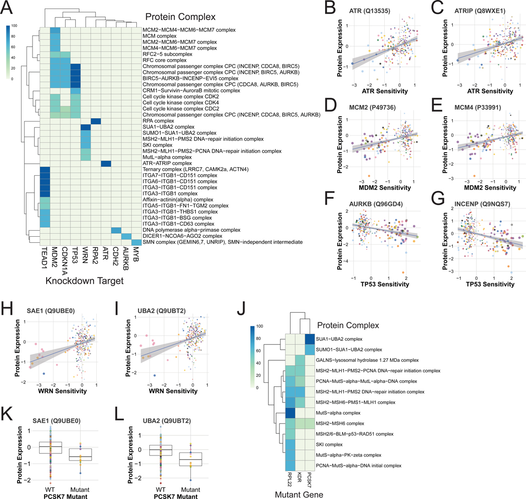
(A) Heatmap of fraction of protein complex members that were significantly associated with sensitivity to shRNA knockdown of different genes. All listed complexes have at least half of their members associated with a knockdown. (B-I) Example associations between gene knockdown sensitivity (x-axis) and protein expression (y-axis). (B) ATR and (C) ATRIP expression compared to sensitivity to ATR knockdown. (D) MCM2 and (E) MCM4 members of the MCM complex compared to MDM knockdown sensitivity. (F) AURKB and (G) INCENP members of the CTR complex compared to sensitivity to TP53 knockdown. (H) SAE1 and (I) UBA2 expression compared to sensitivity to WRN knockdown. (J) Fractions of protein complex members associated with specific gene mutations. (K-L) Expression of (K) SAE1 and (L) UBA2 compared to PCSK7 mutation status. Boxplots are as in Figure 5. Scatterplot trendlines are linear regression with the 95% Cl shaded grey.

Sensitivity to knockdown of TEAD1 was associated with several integrin complexes containing ITGB1 (Fig. 7A). TEAD1 is a transcription cofactor of the YAP1 oncogene, both of which are members of the Hippo signaling pathway that acts downstream of mechanical sensors at the cell surface (Elbediwy and Thompson, 2018; Elbediwy et al., 2016), in agreement with this result.

Three related proteins found by this analysis were TP53, MDM2, and CDKN1A (Fig. 7A). In line with the known functions of these genes, the complexes associated with their knockdown were all tied to cell division including the Chromosomal Passenger Complex (CPC) and CDK-containing complexes. A unique association for MDM2 knockdown sensitivity was with MCM complex levels (Fig. 7A, D-E). Although MDM2 is best known as a negative regulator of TP53, it has TP53-independent functions (Nag et al., 2013), possibly including a relationship with the MCM complex.

As expected, this analysis recovered the mismatch repair and SKI complexes associated with sensitivity to WRN knockdown (Fig. 7A) as well as a complex not associated with MSI status: the SUMO El heterodimer SAE1 and UBA2 (Fig. 7A, H-I). SUMOylation has a function in the cell cycle and DNA damage (Eifler and Vertegaal, 2015), fitting with the known function of WRN. An additional analysis of protein complex changes associated with individual mutations recovered the mismatch repair and SKI complexes associated with RPL22 mutation as well as KDR as described above (Figs. 6E, 7J). However, the SUMO El heterodimer was uniquely associated with mutations in the serine endopeptidase PCSK7 (Fig. 7J-L). PCSK7 was associated with some of the proteins altered by MSI (Fig. 6E) but does not have a known association with it or SUMO.

Discussion

Proteomics has only recently matured to being able to generate reasonably accurate quantitation of the majority of expressed proteins across hundreds of samples. Thus our expectations for the global organization of these proteomes were based on the well-established importance of originating tissue and mutation in cancer. We were thus surprised to find that they could not explain the hierarchical clustering or first principal component. Our analysis demonstrates that a fundamental organizing principle of the proteome is the coordinated expression between pathways, and that this broad organization has correlation with about 75% of expressed proteins. Comparison to RNA demonstrates that this is primarily a property of the proteome, and thus why it has not been described from the extensive transcriptomic analyses performed to date.

Given the massive number of proteins with correlated expression, we expected many protein expression changes associated with mutation at either the level of total mutation burden in MSI or individual genes. In the case of MSI, even though there are at least an order of magnitude more mutations than the average tumor there were surprisingly few consistently altered proteins, but they had coherency around control of DNA mutation and translation input and output. As in the PCA analysis, there was substantial buffering of transcript changes. Because driver mutations are causal for cancer it raises a question: what is the role of proteomic buffering of the transcriptomic changes induced by those driver mutations? The coherency of protein expression across different pathways allows for the hypothesis that the levels of these proteins are actively coordinated to withstand the variety of transcriptomic perturbations caused by oncogenic and passenger mutations, thereby preserving cellular functions. Because many posttranscriptional regulatory pathways exist the underlying mechanisms are likely diverse, complicated, and partially redundant. We hypothesize that intervention to disrupt the buffering capacity of the proteome against the effects of mutation offers new avenues for treatment.

Although MSI has been well studied including in proteomic studies, our results uncovered some surprises. The SKI complex, LTN1, RPL22, and RPL22L1 are resident on the ribosome. The unique association of RPL22 mutation with MSI in the CCLE is intriguing and poorly understood. RPL22 expression levels correlate closely with the SKI complex, and it is possible that RPL22 mutation might be upstream of SKI complex downregulation. The role of the SKI and RQC complexes in MSI disease has not been described, but one possibility is that their downregulation allows the expression of important genes bearing passenger mutations, alleviating the negative selective effects of high mutation burden.

STAR Methods

Lead Contact and Materials Availability

Further information and requests for resources and reagents should be directed to and will be fulfilled by the Lead Contact, Steven Gygi (steven_gygi@hms.harvard.edu). This study did not generate new unique reagents.

Experimental Model and Subject Details

Cell lines within the full CCLE collection were selected based on achieving wide representation of tissues of origin and reasonable representation of the distribution of tissues and driver mutations present in the full collection. Additionally, cell lines present in the NCI60 were largely excluded in favor of less well characterized lines, and cell lines overlapping with the DRIVE and Achilles efforts were emphasized. Cell lines were cultured as done previously (Barretina et al., 2012) according to their recommended optimal conditions. Complete cell line annotations are available as distributed by the CCLE (Ghandi et al., 2019). All cell lines were authenticated prior to processing for mass spectrometry using SNP-based DNA fingerprinting.

Method Details

Sample Preparation

Cell lines were blocked in to multiplex experiments to distribute tissues of origin as evenly as possible with the available cell pellets. Cell lines were cultured as done previously (Barretina et al., 2012) and scraped in PBS on ice, spun down and snap frozen in liquid nitrogen after excess liquid was removed. Cell pellets were lysed in 2% SDS, 150mM NaCL, 50mM Hepes (pH 8.5–8.8), Roche complete EDTA-Free protease inhibitor, and Roche PhosSTOP, 5mM DTT, and 200uM Sodium Vanadate via homogenizer drill (~1mg/mL). Samples were spun down (1000xg for 10min), and reduced for 60 minutes at 37C. After cooling to room temperature samples were alkylated with iodoacetamide (14mM final) for 45 minutes in the dark, and quenched for 15 minutes with DTT (5mM final) in the dark. Protein was isolated from the lysates via methanol-chloroform protein extraction (1 part lysate: 3 parts methanol: 1 part chloroform: 2.5 parts H₂O).

The isolated protein was reconstituted in 8M urea via homogenizer drill and spun down at 2,000xg for 5 minutes. A BCA assay determined the protein level in each sample in triplicate. 5mg of each sample were digested overnight with Lys-C (1:100 enzyme: protein, Wako Chemicals) in 4M urea at 37C and digested again with Trypsin (1:100 enzyme: protein, Thermo) in 1M urea for 5 hours at 37C (concentration of urea was adjusted with 25mM Hepes pH 8.5). Samples were acidified with 20% acetic acid (pH was reduced to ~2–3). 5 mg of digested peptides were desalted in 200mg C18 Sep-Pak columns (Waters) and eluates were dried via speedvac. Dried peptides were resuspended in 200mM EPPS pH 8.0 (~0.5 mg/mL) and peptide level was quantified using the Quantitative Colorimetric Peptide Assay (Pierce) in triplicate.

100ug of peptide in 200mM EPPS pH 8.0 were labeled with TMT10 reagents (6.5ug TMT/lug sample) in a 30% final concentration of acetonitrile for an hour followed by 15 minutes of quenching with 5% hydroxylamine. The reactions were acidified with 20% formic acid (pH reduced to ~2–3). The labeled samples were normalized via “ratio check” via MS using 2ug aliquot of each channel. Each 10-plex consists of 9 samples and a bridge channel used for normalization. The bridge sample was constructed by pooling protein lysates from 11 cell lines (NCIH446, DMS79, NCIH460, DMS53, NCIH69, HCC1954, CAMA1, KYSE180, NMCG1, UACC257, and AU565) to represent the diversity of proteins expressed in different cell lines.

The labeled channels were then combined according to normalization factors produced by the ratio check, diluted in 1% formic acid (reduced acetonitrile concentration to 5%), and desalted in a 50mg SEPPAK column (Waters). The eluate was dried via speedvac.

The labeled 10-plex peptide samples were then resuspended in 1mL of Buffer A (5% acetonitrile, 10mM ammonium bicarbonate pH 8.0) and half was used (~500ug) for HPLC fractionation. 96 fractions were collected and then combined into 24 fractions. The 24 fractions were dried via speedvac and the even fractions were desalted in stage tip columns. Desalted samples were resuspended in 5% acetonitrile, 5% formic acid for LC-MS.

Bridge samples were prepared up front using the above protocol through digestion and desalting, followed by peptide quantification by BCA assay. Equal amounts of each line were combined to make 100mg of total protein prior to digestion. 200ug aliquots of the bridge mixture were frozen and subsequently used for each mutltiplex at the labeling step. The bridge was always labeled with the 131 reagent.

Mass Spectrometry

Samples were run on either a Thermo-Fisher Orbitrap Fusion or Orbitrap Fusion Lumos. MSI data were collected in the Orbitrap using a 120k resolution over an m/z range of 350–1350 setting the maximum injection time to 100ms. Determined charge states between 2 and 6 were required for sequencing, and a 60s dynamic exclusion window was used with isotopes excluded. MS2 sequencing was performed in the ion trap following quadrupole selection and CID fragmentation. The m/z window used during sequencing was 400–2000. MS3 quantification scans were performed using SPS selection (McAlister et al., 2014) of 10 notches from the MS2 spectrum and HCD fragmentation and readout in the Orbitrap at a 50k resolution and a maximum injection time of 150ms. All data were collected in positive ion mode and were centroided online. The analysis of each 10-plex representing 12 fractions with 3hr MS runs consumed 36 hr or ~4 hr per cell line. There were 42 10-plexes across the entire experiment. Because of the scale of the data, all raw files will be available to the community upon request via a hard drive transfer.

Processing of Mass Spectrometry Data

Raw files were initially converted to mzXML for processing. The search database was constructed using the human proteome downloaded from Uniprot on February 4, 2014 containing both SwissProt and TrEMBL entries. It was concatenated onto a database of common contaminants (eg. Trypsin, Human Keratins). The database was sorted in order of contaminants, then SwissProt, then TrEMBL entries, and then sorted by protein length within each of these categories to prioritize protein ID assignments. This database was then reversed and appended to the sorted version to enable target-decoy FDR estimation. Individual spectra were converted to DTA files and searched using Sequest (Eng et al., 1994). The Sequest search parameters included a 20 ppm precursor mass tolerance, 1.0 fragment ion tolerance, and up to 2 internal cleavage sites. Up to 3 oxidized methionines per peptide were allowed as the only differential modification. Static modifications included Cysteine alkylation and TMT on lysine residues and the peptide N-terminus. Cleavages were allowed following lysines and arginines with no proline restriction.

Target-decoy-based FDR estimates (Elias and Gygi, 2007; Peng et al., 2003) were performed using a linear discriminant analysis (LDA) method utilizing XCorr, deltaCN, missed cleavages, PPM, peptide length, and charge state as features. +1 peptides were excluded, as were peptides below a length of 7 and an XCorr of 1. The model was trained using the forward and reverse hits as positive and negative training data. Forward hits with outside 3 standard deviations from the average PPM estimate were also marked as negative examples. Peptides were filtered using LDA-based estimates to a 1% FDR. Each run was filtered separately.

Protein-level FDR was subsequently estimated at the entire dataset level of 504 runs (42 batches of 12 fractions each). For each protein across all samples, the posterior probabilities reported by the LDA model for each peptide were multiplied to give a protein-level probability estimate. Using the Picked FDR method (Savitski et al., 2015) proteins were filtered to the target 1% level. Subsequently, protein identifications were collapsed to a minimal number of identified proteins using the maximum parsimony principle. See Huttlin et al., 2010 for further details.

Common Bioinformatics

All common bioinformatics analyses were performed using R including data normalization and plotting (R Core Team, 2018). Some specific libraries used for plotting include ggplot2 (Wickham, 2009), pheatmap, ggrepel (Slowikowski, 2018), dendextend (Galili, 2015), and UpSetR (Gehlenborg, 2017). Network graphics were generated in Cytoscape (Shannon et al., 2003).

A primary tool for several analyses in this work are various gene set databases taken from MSigDB (Liberzon et al., 2011, 2015). The set we collectively refer to as “pathways” was a combination of the curated gene sets (c2) and hallmark (h) gene sets from MSigDB. GO annotations were also taken from MSigDB (c5) or BioConductor’s org.Hs.eg.db annotations package. The annotations from MSigDB were used for GSEA while BioConductor’s were used for standard GO enrichment testing. Transcription factor binding targets were also from MSigDB (the c3 TFT set). Gene sets used in specific analyses are described in the relevant section.

GO enrichments were performed using the GOstats package (Falcon and Gentleman, 2007). Gene Set Enrichment Analysis was performed using the fgsea package (Sergushichev).

Hierarchical Clustering

Hierarchical clustering of samples was performed on all proteins quantified in all samples in both the replicate and full studies. The distance metric used was Euclidean and the clustering method was Ward’s minimum variance metric. The RNA expression clustering in Figure 2A used only genes where a corresponding protein was quantified in all samples and used in the protein clustering. Gini purity was calculated for each dendrogram after cutting the clustering in to 22 groups, one for each tissue of origin in the full set. Purity was calculated for each cluster as the sum over the squared fraction of a given tissue of origin making up that cluster.

Correlation Network Construction

The correlation network was constructed using R’s cor() function using the pairwise complete observations option to allow for missing data. Correlations using fewer than 99 data points (9 ten-plex experiments) were subsequently removed. FDRs were estimated using the fdrtool package, which gave more conservative results than Benjamini-Hochberg corrections, and edges were filtered to an estimated 1% FDR. This process was performed for all 375 cell lines as well as only solid organ-derived lines, and the latter showed much better overall correlations with a more dense and informative network. Thus, only the solid organ-derived lines were used for the final reported network and subsequent annotation networks.

The same procedure was used to compute networks from the RNASeq, Project DRIVE shRNA, and Project Achilles CRISPR datasets. In the case of the RNASeq data, only genes quantified at least once in the protein data were considered. Shared links between these networks and the protein correlation network were used to annotate edges on the protein correlation network.

To annotate putative protein interactions, we used the BioPlex 2.0 network for both direct links and reported community memberships (Huttlin et al., 2017). Additional physical interactions were taken from public databases Biogrid (which includes the BioPlex results) as well as CORUM (Giurgiu et al., 2019).

Annotation for localization used several hand curated databases where possible. Mitochondrial proteins were taken from the Mitocarta 2.0 release. Peroxisome genes were from PeroxisomeDB 2.0 (Schlüter et al., 2010). Lysosome genes were downloaded from the Human Lysosome Gene Database (Brozzi et al., 2013). Ribosome annotations were from UniProt. ER, Golgi, and Ribosome annotations were downloaded from UniProt. Shared localizations from these gene sets were used to annotate edges. Localizations predicted from BioPlex 2.0 shared between nodes were also annotated.

UniProt was used as a general source of annotations after processing. Many proteins contained multiple localizations, and many localization terms had parent terms. Our goal was to reduce the number of localizations to a reasonable subset grouped by parent terms at the specificity of about an organelle or relatively large microscopic structure. All subcellular annotations and their parent localization terms were extracted from UniProt using the SPARQL endpoint. We manually assembled parent level terms to include the following: “Cell Junction”, “Cell Membrane”, “Cell Projection”, “Cilium”, “Cytoskeleton”, “Cytoplasm”, “Cytoplasmic Vesicle”, “Endoplasmic Reticulum”, “Endosome”, “Flagellum”, “Golgi Apparatus”, “Lipid Droplet”, “Lysosome”, “Melanosome”, “Membrane”, “Mitochondrion”, “Nucleus”, “Peroxisome”, “Secreted”, and “Vacuole”. After all protein localizations were downloaded from UniProt for the proteins in our dataset, localizations were collapsed down to one or more of those parent localizations by walking up the tree from each annotation until it reached one of those parent terms. Additionally, any “Membrane” annotations were considered as too unspecific and were removed. Shared localizations according to these parent annotations were annotated on the correlation network edges in their own category.

Finally, a composite annotation count by localization from the gene sets, BioPlex predictions, and collapsed UniProt entries was computed and shown in Figure S5B.

Complex membership in Figure S5D was extracted from CORUM.

Our annotation for putative mechanisms used simple methods, but more advanced approaches such as Bayes Nets or partial correlations could achieve improved mechanistic evidence should they be attempted.

Quantification and Statistical Analysis

Mass Spectrometry Data Quantification and Normalization

For quantification, TMT signal-to-noise values were extracted from the MS3 scans and paired with the MS2 peptide identifications. Peptides were filtered for a summed signal-to-noise of 200 across all 10 TMT channels and an isolation specificity of at least 0.5 in the MSI isolation window. For each protein, the filtered peptide TMT values were summed to create non-normalized protein quantifications. To control for differential protein loading within a ten-plex, the summed protein quantities were adjusted to be equal within a ten-plex. Following this, values were log2-transformed, and within each ten-plex the bridge channel protein quantity was subtracted from each sample quantity to create a ratio to the bridge. Bridge samples, now 0, were removed. For each protein, there is some measurement error in the measurement of the bridge sample. To account for this, within each ten-plex, the mean protein expression was centered at 0. Finally, ten-plexes were joined by protein identification to create the complete data set.

Our normalization procedure was assessed qualitatively and quantitatively before arriving at the method described above. Multiple diagnostics were used on both the first 6 ten-plexes and then, subsequently, on the full dataset to compare normalization approaches. The primary diagnostics used were cohesive hierarchical clustering assessed both visually and by Gini purity of tissue lineage clustering, linear modeling of replicate and tissue-based effects across the dataset, and correlation of RNA and protein expression. Additionally, defects in normalization at different stages of the work were found visually, explored, and corrected using the methods described above. The final normalization procedure biased towards simple adjustments over more complex approaches to favor general interpretability and reproducibility. For example, although it is frequently used in proteomics, imputation was not used in these data because the assumptions inherent in any imputation methods on multiplexed data hindered the interpretation of the final data set in comparison to simply providing missing values where no measurements were successfully completed.

Principal Components Analysis

Principal components analysis was performed using proteins quantified in all samples, and the number of significant components was estimated by the broken stick model using the vegan R package (Oksanen et al., 2018). Loadings for the all proteins were used to perform GSEA (Subramanian et al., 2005) using the gene sets described above. Significantly enriched gene sets were considered at an FDR of 1% or less. Individual heatmaps for example data sets were generated using the leading edge proteins from selected significant pathway. Duplicate entries across pathways in the same heatmap were removed so each protein was only plotted once.

For the Upset plots in Figure 4B-D, the above PCA was performed on the CCLE protein and RNASeq data separately and the overlap of significantly enriched gene sets in each data set’s separate PC1 was plotted.

Much of the same analysis was repeated using Independent Components Analysis using the ica R package implementing the FastICA algorithm (Helwig, 2018). Both the projections of the cell lines and gene set enrichment analysis of the loadings of the first column of the mixing matrix M produced similar results to the PCA-based analysis above.

Correlation Analyses

Correlations between protein and gene expression values were performed either by sample or by gene. Correlations by sample were performed using Pearson correlation across all RNA expression levels from the CCLE RNASeq data where a protein was quantified in at least one ten-plex (9 cell lines). To generate the heatmap in Figure 2B the same axis ordering was applied to both protein and RNA samples.

All protein expression levels were correlated to the PC1 projection for each cell line. Tests of significance were done using cor.test() and p-values were filtered to a 1% FDR as estimated by fdrtool. Protein expression levels for EPCAM and VIM were correlated with all protein or mRNA expression measurements using R’s cor.test() function. FDRs were estimated using fdrtool and filtered to a 1% FDR before partitioning in to significant and positively or negatively associated with each expression type.

Mutation Analysis

All regressions were performed using standard linear regression implemented by R’s lm() function unless otherwise specified.

Total mutational burden for a cell line was taken as the total number of mutations called excluding common alleles. For Figure S2C this was regressed against the PC1 projection for each cell line using a basic linear model with no additional covariates. Attempts to select mutations predictive for PC1 projection shown in Figure S2D was performed using commonly mutated genes in cancer as identified by Vogelstein and colleagues (Vogelstein et al., 2013). Mutations in cell lines derived from solid organ (non-haematopoetic and non-lymphoid) lineages were filtered to those genes. At least 5 identified mutations in the cell lines in our data set were required to provide some minimal power level. For variable selection we used an elastic net with 10 repeats of 10-fold cross validated fitting and validation. Optimal model parameters were chosen by minimizing RMSE across all repeats and folds. The selected genes with the highest estimated importance to the model were plotted in Figure S2D, except TP53 which is mutated in most cell lines and distorts the histograms for all other genes. Parameter tuning and model fitting was performed using the caret and glmnet packages (Friedman et al., 2010; Kuhn, 2008).

Individual mutations were regressed against protein expression also using tissue and sex as covariates without interaction terms. Mutations were limited to nonsilent and uncommon mutations in genes listed in the Cancer Gene Census. At least 10 cell lines bearing a relevant mutation needed corresponding protein measurements to perform each regression. P-values for the effect of the mutation were computed and FDRs were estimated using fdrtool and filtered to a 5% level.

Sensitivity Analysis

All regressions were performed using standard linear regression implemented by R’s lm() function unless otherwise specified.

CRISPR scores were taken from the Avana dataset (Meyers et al., 2017) from depmap.org (18Q3 release on August 6, 2018), shRNA data was taken from Project DRIVE (McDonald et al., 2017) and drug treatment data was taken from the CTD2 dataset (Basu et al., 2013). Pearson correlation values between these scores and the sample PC1 projection was performed only in cases where there were at least 30 complete pairwise data points available. P-values were calculated using R’s cor.testQ function, and FDR was estimated using fdrtool.

Per-protein associations with cell sensitivities were assessed using the DRIVE dataset. Linear regressions were performed for every protein against every DRIVE score using tissue and sex as covariates and no interaction terms. At least 100 overlapping protein quantitiations and knockdown sensitivity scores were required for each regression. P-values associated with protein expression were computed and FDRs were filtered to a 5% level after estimation using fdrtool.

MSI Analysis

MSI status was as inferred in the previous CCLE analysis (Ghandi et al., 2019). For each protein, expression was regressed against MSI status, tissue, and sex and FDR was estimated using fdrtool. At least 100 samples with protein measurements were required for each regression. The significance threshold was 5% FDR. The same regression was repeated using RNASeq expression in place of protein to produce the overlap. Significant hits were assessed for relationships using STRING and high confidence relationships (score > 0.7) were extracted for figure 5B. The expression of the significant proteins quantified in all samples were correlated in both MSI lines alone and non-haematopoetic or lymphoid MSS lines to produce the heatmaps in Figure 6A-B.

To assess the effect of mutation burden on the clustering, for the 50 proteins significantly altered in MSI lines expression levels were separately regressed in one of three models. One model used MSI status alone, the second used estimated sample mutation burden alone, and one used the interaction between the two. All three models also used tissue and sex as covariates. AIC and BIC were estimated for all fits and BIC minimization was ultimately used as the selected goodness of fit measure after manual inspection of the results. Selected proteins where mutation burden was present in the best fit model are shown in figure 6D and selected proteins where mutation burden is absent in the best fit model are shown in figure 6C. These fits are also performed and plotted in figure 6F.

The network plot in figure 6E summarizes a subset of individual regressions of protein expression against individual mutations described above. Proteins significantly altered in MSI that were also significantly altered by individual mutations were extracted from the results and plotted as a directed network in Cytoscape. The source node was plotted as the mutated gene while the end node was the protein with altered expression. Any mutant gene affecting a protein also altered in MSI is plotted.

All histone modification marks from the CCLE were regressed against MSI versus non-MSI status, incorporating tissue and sex as additional covariates. FDR was estimated using fdrtool. H3K4 methylation marks were among the significant hits and are plotted in figure 6I.

Protein Complex Relationship to Sensitivity and Mutation

Protein complex gene sets were taken from the CORUM database (Giurgiu et al., 2019). Associations with protein complexes were restricted to knockdown targets with large numbers of large effects. These were genes in at least the 90^th percentile of norm-LRT scores (McDonald et al., 2017) and at least 5 samples with a sensitivity score less than −1 or greater than 1, with at least one such score less than −2 or greater than 2. Among the protein expression/gene knockdown associations protein complexes from CORUM with at least 50% of the annotated members significantly associated with a knockdown were annotated in Figure 7. Mutations were not restricted beyond the set described above, and the same 50% of the complex criterion was used to annotate those associations.

Supplementary Material

FS1

Figure S1: Numbers of proteins quantified per ten-plex and their overlap, Related to Figure 1. (A) Summary statistics for the data set. (B) Numbers of proteins quantified in each ten-plex. The median level is denoted by the dashed line. (C) Numbers of proteins quantified across each number of ten-plexes. Over 5,000 proteins were quantified in all 42 ten-plexes, and only 151 were quantified in a single ten-plex. The results shown in this plot are summarized in Figure 1B. (D) Coverage of different sets of proteins. Bars are colored by fraction of proteins quantified in differe nt numbers of samples. For example, nearly all mitochondrial proteins were quantified in all samples while about half of all transcription factors were quantified in at least one sample. No olfactory receptors were quantified.

FS2

Figure S2: Features associated with pathway coexpression of the proteome, Related to Figures 3–4. (A) PCA of the haematopoetic and lymphoid lineages alone shows them mostly segregating from each other based on the first two principal components. (B) Heatmap of large protein complexes found to be enriched in the protein PC1. Axes and annotations are the same as in Figure 3C. (C) Scatter plot of solid organ lineage cell lines comparing PC1 projection (x-axis, same as in Figure 3B) with total mutational burden of uncommon alleles. The linear regression along with 95% confidence interval is plotted. (D) The top mutations predicting the PC1 projection of a cell line were selected by elastic net. The top 12 excluding TP53 (which is has mutations in most cell lines) are plotted. Each subpanel is a histogram where cell lines are binned along their PC1 projections. If a cell line has an uncommon allele in the gene of interest it is plotted as a stacked bar in that bin. The bar is colored by tissue of origin. For example, VHL mutations are predominantly in kidney lines (orange) and cluster in the negative PC1 projections. Dashed black lines denote the 0 point along PC1, and the dashed blue lines are the gene-specific median. (E) Expression levels of RNASeq (left) and protein (right) for various transcription factor targets. Transcription factors targeting these proteins are annotated on the bottom according to the legend. Samples are arranged along the PCA PC1 projection, similarly to Figures 3 and 4, but performing the PCA on the RNASeq data instead of the protein data, resulting in a different ordering of samples. Correlation between RNA and protein is annotated on the bottom of the protein panel.

FS3

Figure S3. A large fraction of the proteome is correlated with the epithelial and mesenchymal markers EPCAM and VIM, Related to Figures 3–4. (A-B) Percentages of proteins and RNA showing significant correlation with the protein expression levels of the epithelial marker EPCAM (A) and mesenchymal marker VIM (B) are shown along with selected significantly enriched GO categories in each partition. Over 40% of quantified proteins show some correlation with EPCAM, and over 30% with VIM. Only non-haematopoetic and lymphoid lineages were used in these computations.

FS4

Figure S4, Related to Figures 3–4. Cell sensitivities associated with proteome expression. (A) Distribution of correlations between the cell line projection in protein PC1 (position on the x-axis in Figure 3B) and sensitivities for individual gene loss by CRISPR or shRNA. Significantly correlated gene sensitivities are shown, with positive correlations shown in red and negative correlations in blue. Bolded names are extracellular proteins, which are enriched in this set. (B) Example significant correlations from the distribution in panel A. (C) Distribution of correlations between the PC1 projection (as in panel A) and drug sensitivities. Red and blue coloring is the same as in panel A. Drugs with significant correlations are listed and colored by some of their known targets. (D) Example scatter plots for the correlations in the histogram in panel C.

FS5

Figure S5, Related to Figures 3–4. A protein expression correlation network captures mechanistic relationships. (A) Overview of the network. (B) Summary statistics for putative mechanistic annotations underlying correlations in the network. Multiple datasets were used to annotate each edge (see Methods) and the number of correlations annotated by each dataset and fraction of total edges with any annotation are shown in the boxes. The cumulative total of all edges with an annotation is shown by the line. (C) Overlap of link explanations that are summarized in panel (B). (D-E) Selected subnetworks. All edges are found via protein correlation in addition to any datatypes annotated by color in the legend. (D) A subset of the correlation network surrounding the epithelial and mesenchymal makers EPCAM and Vimentin. Around these nodes are proteins involved in epithelial or mesenchymal biology. All green edges were also in the RNASeq correlation network. (E) Some protein complexes in the protein correlation network. All blue and yellow lines were also in a protein-protein interaction database. All red and yellow lines were found in a gene loss sensitivity correlation network. See also Table S4.

FS6

Figure S6: Significant protein expression changes associated with mutations in selected genes, Related to Figures 5–7. The volcano plots show the estimated value of the coefficient from the linear model (x-axis) against the -loglO of the nominal p-value for that term in the model (y-axis). The effects of the mutation in each gene is shown at the top of each panel, and the points on the plot are proteins whose expression is tested against the mutation. In all cases except KDR (D) significant hits are labeled and plotted in black. For KDR, too many points are significant to visualize with labels, so only those proteins that are either in the Cancer Gene Census list or are also significant in RPL22 mutants (C) are labeled. See also Table S7.

TS1

Supplemental Table SI. Cell line information, Related to all Figures.

TS2

Supplemental Table S2. Normalized protein expression levels, Related to all Figures.

TS3

Supplemental Table S3. Normalized protein expression levels in biological replicate samples, Related to Figure 1.

TS4

Supplemental Table S4. Protein/mRNA correlation and gene set enrichment results, Related to Figure 2.

TS5

Supplemental Table S5. Gene set enrichment results for solid lineage PCA PC1 protein loadings, Related to Figures 3–4.

TS6

Supplemental Table S6. Correlation network of protein expression levels in solid tissue-derived lineages, Related to Figures 3–4.

TS7

Supplemental Table S7. Statistical associations between individual gene mutations and protein expression levels, Related to Figures 5–7.

Key Resources Table

REAGENT or RESOURCE	SOURCE	IDENTIFIER
Chemicals, Peptides, and Recombinant Proteins
Roche complete, EDTA-free	Sigma	Cat# 11 873 580 001
Roche PhosSTOP	Sigma	Cat# 04 906 837 001
Pierce Trypsin Protease, MS Grade	ThermoFisher	Cat# 90058
Lys-C, Mass Spectrometry Grade	Wako Chemicals	Barcode# 4987481427648
TMT 10-Plex	ThermoFisher	Cat# 90406
Critical Commercial Assays
Pierce Quantitative Colorimetric Peptide Assay	ThermoFisher	Cat# 23275
Software and Algorithms
Sequest	ThermoFisher	Eng et al., 1994
R	R Project	https://www.r-project.org/
ggplot2	CRAN	https://ggplot2.tidyverse.org/index.html
ggrepel	CRAN	https://github.com/slowkow/ggrepel
pheatmap	CRAN	https://cran.r-project.org/web/packages/pheatmap/index.html
dendextend	CRAN	https://github.eom/talgalili/dendextend/
UpSetR	CRAN	https://github.com/hms-dbmi/UpSetR
MSigDB	The Broad Institute	http://software.broadinstitute.org/gsea/msigdb/index.jsp
GOstats	Bioconductor	https://bioconductor.org/packages/release/bioc/html/GOstats.html
fgsea	Bioconductor	https://bioconductor.org/packages/release/bioc/html/fgsea.html
fdrtool	CRAN	http://www.strimmerlab.org/software/fdrtool/
Cytoscape	Cytoscape Consortium	https://cytoscape.org/
Other
Waters 200mg Sep-Pak	Waters	Prod# WAT054945
Waters 50mg Sep-Pak	Waters	Prod# WAT054955
Orbitrap Fusion	ThermoFisher	Cat# IQLAAEGAAPFADBM BCX
Orbitrap Fusion Lumos	ThermoFisher	Cat# IQLAAEGAAPFADBM BHQ

• Quantified the proteomes of 375 cell lines from diverse lineages in the CCLE

• Correlated expression of proteins across many pathways

• Downregulation of multiple protein complexes in microsatellite instability (MSI)

• Protein complexes associated with sensitivity to gene knockdown and mutation

References

- Baretti M, and Le DT (2018). DNA mismatch repair in cancer. Pharmacology & Therapeutics 189, 45–62. [DOI] [PubMed] [Google Scholar]
- Barretina J, Caponigro G, Stransky N, Venkatesan K, Margolin AA, Kim S, Wilson CJ, Lehár J, Kryukov GV, Sonkin D, et al. (2012). The Cancer Cell Line Encyclopedia enables predictive modelling of anticancer drug sensitivity. Nature 483, 603–307. [DOI] [PMC free article] [PubMed] [Google Scholar]
- Basu A, Bodycombe NE, Cheah JH, Price EV, Liu K, Schaefer GI, Ebright RY, Stewart ML, Ito D, Wang S, et al. (2013). An Interactive Resource to Identify Cancer Genetic and Lineage Dependencies Targeted by Small Molecules. Cell 154,1151–1161. [DOI] [PMC free article] [PubMed] [Google Scholar]
- Behan FM, lorio F, Picco G, Gonçalves E, Beaver CM, Migliardi G, Santos R, Rao Y, Sassi F, Pinnelli M, et al. (2019). Prioritization of cancer therapeutic targets using CRISPR-Cas9 screens. Nature 568, 511. [DOI] [PubMed] [Google Scholar]
- Brandman O, Stewart-Ornstein J, Wong D, Larson A, Williams CC, Li G-W, Zhou S, King D, Shen PS, Weibezahn J, et al. (2012). A Ribosome-Bound Quality Control Complex Triggers Degradation of Nascent Peptides and Signals Translation Stress. Cell 151,1042–1054. [DOI] [PMC free article] [PubMed] [Google Scholar]
- Brozzi A, Urbanelli L, Luc Germain P, Magini A, and Emiliani C. (2013). hLGDB: a database of human lysosomal genes and their regulation. Database (Oxford) 2013. [DOI] [PMC free article] [PubMed] [Google Scholar]
- Campbell BB, Light N, Fabrizio D, Zatzman M, Fuligni F, Borja R. de, Davidson S, Edwards M, Elvin JA, Hodel KP, et al. (2017). Comprehensive Analysis of Hypermutation in Human Cancer. Cell 171,1042–1056.elO. [DOI] [PMC free article] [PubMed] [Google Scholar]
- Cao B, Fang Z, Liao P, Zhou X, Xiong J, Zeng S, and Lu H. (2017). Cancer-mutated ribosome protein L22 (RPL22/eL22) suppresses cancer cell survival by blocking p53-MDM2 circuit. Oncotarget 8, 90651–90661. [DOI] [PMC free article] [PubMed] [Google Scholar]
- Caron H, Schaik B. van Mee M.van der Baas F, Riggins G, Sluis P. van, Hermus M-C, Asperen R. van Boon K, Voûte PA, et al. (2001). The Human Transcriptome Map: Clustering of Highly Expressed Genes in Chromosomal Domains. Science 291,1289–1292. [DOI] [PubMed] [Google Scholar]
- Causse SZ, Marcion G, Chanteloup G, Uyanik B, Boudesco C, Grigorash BB, Douhard R, Dias AMM, Dumetier B, Dondaine L, et al. (2019). HSP110 translocates to the nucleus upon genotoxic chemotherapy and promotes DNA repair in colorectal cancer cells. Oncogene 38, 2767–2777. [DOI] [PubMed] [Google Scholar]
- Chan EM, Shibue T, McFarland JM, Gaeta B, Ghandi M, Dumont N, Gonzalez A, McPartlan JS, Li T, Zhang Y, et al. (2019). WRN helicase is a synthetic lethal target in microsatellite unstable cancers. Nature 568, 551. [DOI] [PMC free article] [PubMed] [Google Scholar]
- Choi YJ, Oh HR, Choi MR, Gwak M, An CH, Chung YJ, Yoo NJ, and Lee SH (2014). Frameshift mutation of a histone methylation-related gene SETD1B and its regional heterogeneity in gastric and colorectal cancers with high microsatellite instability. Human Pathology 45, 1674–1681. [DOI] [PubMed] [Google Scholar]
- Dephoure N, Hwang S, O’Sullivan C, Dodgson SE, Gygi SP, Amon A, and Torres EM (2014). Quantitative proteomic analysis reveals posttranslational responses to aneuploidy in yeast. ELife 3, e03023. [DOI] [PMC free article] [PubMed] [Google Scholar]
- Dixon JR, Gorkin DU, and Ren B. (2016). Chromatin Domains: The Unit of Chromosome Organization. Molecular Cell 62, 668–680. [DOI] [PMC free article] [PubMed] [Google Scholar]
- Dorard C, de Thonel A, Collura A, Marisa L, Svrcek M, Lagrange A, Jego G, Wanherdrick K, Joly AL, Buhard O, et al. (2011). Expression of a mutant HSP110 sensitizes colorectal cancer cells to chemotherapy and improves disease prognosis. Nature Medicine 17,1283–1289. [DOI] [PubMed] [Google Scholar]
- Edfors F, Danielsson F, Hallström BM, Käil L, Lundberg E, Ponten F, Forsström B, and Uhlén M. (2016). Gene-specific correlation of RNA and protein levels in human cells and tissues. Molecular Systems Biology 12, 883. [DOI] [PMC free article] [PubMed] [Google Scholar]
- Eifler K, and Vertegaal ACO (2015). SUMOylation-mediated regulation of cell cycle progression and cancer. Trends Biochem Sci 40, 779–793. [DOI] [PMC free article] [PubMed] [Google Scholar]
- Elbediwy A, and Thompson BJ (2018). Evolution of mechanotransduction via YAP/TAZ in animal epithelia. Current Opinion in Cell Biology 51, 117–123. [DOI] [PubMed] [Google Scholar]
- Elbediwy A, Vincent-Mistiaen ZI, and Thompson BJ (2016). YAP and TAZ in epithelial stem cells: A sensor for cell polarity, mechanical forces and tissue damage. BioEssays 38, 644–653. [DOI] [PMC free article] [PubMed] [Google Scholar]
- Elias JE, and Gygi SP (2007). Target-decoy search strategy for increased confidence in large-scale protein identifications by mass spectrometry. Nat Meth 4, 207–214. [DOI] [PubMed] [Google Scholar]
- Eng J, McCormack A, and Yates J. (1994). An approach to correlate tandem mass spectral data of peptides with amino acid sequences in a protein database. Journal of The American Society for Mass Spectrometry 5, 976–989. [DOI] [PubMed] [Google Scholar]
- Eshleman JR, and Markowitz SD (1996). Mismatch repair defects in human carcinogenesis. Hum Mol Genet 5, 1489–1494. [DOI] [PubMed] [Google Scholar]
- Falcon S, and Gentleman R. (2007). Using GOstats to test gene lists for GO term association. Bioinformatics 23, 257–258. [DOI] [PubMed] [Google Scholar]
- Frejno M, Chiozzi RZ, Wilhelm M, Koch H, Zheng R, Klaeger S, Ruprecht B, Meng C, Kramer K, Jarzab A, et al. (2017). Pharmacoproteomic characterisation of human colon and rectal cancer. Molecular Systems Biology 13, 951. [DOI] [PMC free article] [PubMed] [Google Scholar]
- Friedman J, Hastie T, and Tibshirani R. (2010). Regularization Paths for Generalized Linear Models via Coordinate Descent. Journal of Statistical Software, Articles 33,1–22. [PMC free article] [PubMed] [Google Scholar]
- Furlong EEM, and Levine M. (2018). Developmental enhancers and chromosome topology. Science 361, 1341–1345. [DOI] [PMC free article] [PubMed] [Google Scholar]
- Galili T. (2015). dendextend: an R package for visualizing, adjusting, and comparing trees of hierarchical clustering. Bioinformatics. [DOI] [PMC free article] [PubMed] [Google Scholar]
- Gehlenborg N. (2017). UpSetR: A More Scalable Alternative to Venn and Euler Diagrams for Visualizing Intersecting Sets. [Google Scholar]
- Ghandi M, Huang FW, Jané-Valbuena J, Kryukov GV, Lo CC, McDonald ER, Barretina J, Gelfand ET, Bielski CM, Li H, et al. (2019). Next-generation characterization of the Cancer Cell Line Encyclopedia. Nature 569, 503. [DOI] [PMC free article] [PubMed] [Google Scholar]
- Gholami AM, Hahne H, Wu Z, Auer FJ, Meng C, Wilhelm M, and Kuster B. (2013). Global Proteome Analysis of the NCI-60 Cell Line Panel. Cell Reports 4, 609–620. [DOI] [PubMed] [Google Scholar]
- Giannini G, Rinaldi C, Ristori E, Ambrosini MI, Cerignoli F, Viel A, Bidoli E, Berni S, D’Amati G, Scambia G, et al. (2004). Mutations of an intronic repeat induce impaired MRE11 expression in primary human cancer with microsatellite instability. Oncogene 23, 2640–2647. [DOI] [PubMed] [Google Scholar]
- Giurgiu M, Reinhard J, Brauner B, Dunger-Kaltenbach I, Fobo G, Frishman G, Montrone C, and Ruepp A. (2019). CORUM: the comprehensive resource of mammalian protein complexes-2019. Nucleic Acids Res. 47, D559–D563. [DOI] [PMC free article] [PubMed] [Google Scholar]
- Gonçalves E, Fragoulis A, Garcia-Alonso L, Cramer T, Saez-Rodriguez J, and Beltrao P. (2017). Widespread Post-transcriptional Attenuation of Genomic Copy-Number Variation in Cancer. Cell Systems 5, 386–398.e4. [DOI] [PMC free article] [PubMed] [Google Scholar]
- Grabowski P, Kustatscher G, and Rappsilber J. (2018). Epigenetic Variability Confounds Transcriptome but Not Proteome Profiling for Coexpression-based Gene Function Prediction. Molecular & Cellular Proteomics 17, 2082–2090. [DOI] [PMC free article] [PubMed] [Google Scholar]
- Gygi SP, Rochon Y, Franza BR, and Aebersold R. (1999). Correlation between Protein and mRNA Abundance in Yeast. Mol. Cell. Biol 19, 1720–1730. [DOI] [PMC free article] [PubMed] [Google Scholar]
- Halbach F, Reichelt P, Rode M, and Conti E. (2013). The Yeast Ski Complex: Crystal Structure and RNA Channeling to the Exosome Complex. Cell 154, 814–826. [DOI] [PubMed] [Google Scholar]
- Halvey PJ, Wang X, Wang J, Bhat AA, Dhawan P, Li M, Zhang B, Liebler DC, and Slebos RJC (2013). Proteogenomic Analysis Reveals Unanticipated Adaptations of Colorectal Tumor Cells to Deficiencies in DNA Mismatch Repair. Cancer Res. [DOI] [PMC free article] [PubMed] [Google Scholar]
- Helwig NE (2018). ica: Independent Component Analysis. [Google Scholar]
- Hnisz D, Shrinivas K, Young RA, Chakraborty AK, and Sharp PA (2017). A Phase Separation Model for Transcriptional Control. Cell 169,13–23. [DOI] [PMC free article] [PubMed] [Google Scholar]
- Huttlin EL, Jedrychowski MP, Elias JE, Goswami T, Rad R, Beausoleil SA, Villen J, Haas W, Sowa ME, and Gygi SP (2010). A Tissue-Specific Atlas of Mouse Protein Phosphorylation and Expression. Cell 143,1174–1189. [DOI] [PMC free article] [PubMed] [Google Scholar]
- Huttlin EL, Bruckner RJ, Paulo JA, Cannon JR, Ting L, Baltier K, Colby G, Gebreab F, Gygi MP, Parzen H, et al. (2017). Architecture of the human interactome defines protein communities and disease networks. Nature 545, 505–509. [DOI] [PMC free article] [PubMed] [Google Scholar]
- Ise N, Omi K, Nambara D, Higashiyama S, and Goishi K. (2011). Overexpressed HER2 in NSCLC is a Possible Therapeutic Target of EGFR Inhibitors. Anticancer Res 31, 4155–4161. [PubMed] [Google Scholar]
- Jovanovic M, Rooney MS, Mertins P, Przybylski D, Chevrier N, Satija R, Rodriguez EH, Fields AP, Schwartz S, Raychowdhury R, et al. (2015). Dynamic profiling of the protein life cycle in response to pathogens. Science 347, 1259038. [DOI] [PMC free article] [PubMed] [Google Scholar]
- Kim JW, Kim H-P, Im S-A, Kang S, Hur HS, Yoon Y-K, Oh D-Y, Kim JH, Lee DS, Kim T-Y, et al. (2008). The growth inhibitory effect of lapatinib, a dual inhibitor of EGFR and HER2 tyrosine kinase, in gastric cancer cell lines. Cancer Letters 272, 296–306. [DOI] [PubMed] [Google Scholar]
- Kuhn M. (2008). Building Predictive Models in R Using the caret Package. Journal of Statistical Software 28,1–26.27774042 [Google Scholar]
- Kustatscher G, Grabowski P, and Rappsilber J. (2017). Pervasive coexpression of spatially proximal genes is buffered at the protein level. Molecular Systems Biology 13, 937. [DOI] [PMC free article] [PubMed] [Google Scholar]
- Lapek JD, Greninger P, Morris R, Amzallag A, Pruteanu-Malinici I, Benes CH, and Haas W. (2017). Detection of dysregulated protein-association networks by high-throughput proteomics predicts cancer vulnerabilities. Nature Biotechnology. [DOI] [PMC free article] [PubMed] [Google Scholar]
- Lawrence MS, Stojanov P, Polak P, Kryukov GV, Cibulskis K, Sivachenko A, Carter SL, Stewart C, Mermel CH, Roberts SA, et al. (2013). Mutational heterogeneity in cancer and the search for new cancer-associated genes. Nature advance online publication. [DOI] [PMC free article] [PubMed] [Google Scholar]
- Li H, Ning S, Ghandi M, Kryukov GV, Gopal S, Deik A, Souza A, Pierce K, Keskula P, Hernandez D, et al. (2019). The landscape of cancer cell line metabolism. Nat Med 25, 850–860. [DOI] [PMC free article] [PubMed] [Google Scholar]
- Li J, Zhao W, Akbani R, Liu W, Ju Z, Ling S, Vellano CP, Roebuck P, Yu Q, Eterovic AK, et al. (2017). Characterization of Human Cancer Cell Lines by Reverse-phase Protein Arrays. Cancer Cell 31, 225–239. [DOI] [PMC free article] [PubMed] [Google Scholar]
- Liberzon A, Subramanian A, Pinchback R, Thorvaldsdóttir H, Tamayo P, and Mesirov JP (2011). Molecular signatures database (MSigDB) 3.0. Bioinformatics 27, 1739–1740. [DOI] [PMC free article] [PubMed] [Google Scholar]
- Liberzon A, Birger C, Thorvaldsdóttir H, Ghandi M, Mesirov JP, and Tamayo P. (2015). The Molecular Signatures Database Hallmark Gene Set Collection. Cell Systems 1, 417–425. [DOI] [PMC free article] [PubMed] [Google Scholar]
- Lieb S, Blaha-Ostermann S, Kamper E, Rippka J, Schwarz C, Ehrenhöfer-Wölfer K, Schlattl A, Wernitznig A, Lipp JJ, Nagasaka K, et al. (2019). Werner syndrome helicase is a selective vulnerability of microsatellite instability-high tumor cells. ELife 8, e43333. [DOI] [PMC free article] [PubMed] [Google Scholar]
- Liu Q, and Zhang B. (2016). Integrative Omics Analysis Reveals Post-Transcriptionally Enhanced Protective Host Response in Colorectal Cancers with Microsatellite Instability. J Proteome Res 15, 766–776. [DOI] [PMC free article] [PubMed] [Google Scholar]
- Liu Y, Beyer A, and Aebersold R. (2016). On the Dependency of Cellular Protein Levels on mRNA Abundance. Cell 165, 535–550. [DOI] [PubMed] [Google Scholar]
- McAlister GC, Nusinow DP, Jedrychowski MP, Wühr M, Huttlin EL, Erickson BK, Rad R, Haas W, and Gygi SP (2014). MultiNotch MS3 Enables Accurate, Sensitive, and Multiplexed Detection of Differential Expression across Cancer Cell Line Proteomes. Anal. Chem 86, 7150–7158. [DOI] [PMC free article] [PubMed] [Google Scholar]
- McDonald ER, Weck A. de, Schlabach MR, Billy E, Mavrakis KJ, Hoffman GR, Belur D, Castelletti D, Frias E, Gampa K, et al. (2017). Project DRIVE: A Compendium of Cancer Dependencies and Synthetic Lethal Relationships Uncovered by Large-Scale, Deep RNAi Screening. Cell 170, 577–592.elO. [DOI] [PubMed] [Google Scholar]
- Mertins P, Mani DR, Ruggles KV, Gillette MA, Clauser KR, Wang P, Wang X, Qiao JW, Cao S, Petralia F, et al. (2016). Proteogenomics connects somatic mutations to signalling in breast cancer. Nature 534, 55–62. [DOI] [PMC free article] [PubMed] [Google Scholar]
- Meyers RM, Bryan JG, McFarland JM, Weir BA, Sizemore AE, Xu H, Dharia NV, Montgomery PG, Cowley GS, Pantel S, et al. (2017). Computational correction of copy number effect improves specificity of CRISPR-Cas9 essentiality screens in cancer cells. Nature Genetics 49,1779–1784. [DOI] [PMC free article] [PubMed] [Google Scholar]
- Mimura K, Kono K, Hanawa M, Kanzaki M, Nakao A, Ooi A, and Fujii H. (2005). Trastuzumab-Mediated Antibody-Dependent Cellular Cytotoxicity against Esophageal Squamous Cell Carcinoma. Clin Cancer Res 11, 4898–4904. [DOI] [PubMed] [Google Scholar]
- Nag S, Qin J, Srivenugopal KS, Wang M, and Zhang R. (2013). The MDM2-p53 pathway revisited. J Biomed Res 27, 254–271. [DOI] [PMC free article] [PubMed] [Google Scholar]
- Novetsky AP, Zighelboim I, Thompson DM, Powell MA, Mutch DG, and Goodfellow PJ (2013). Frequent mutations in the RPL22 gene and its clinical and functional implications. Gynecologic Oncology 128, 470–474. [DOI] [PMC free article] [PubMed] [Google Scholar]
- Oksanen J, Blanchet FG, Friendly M, Kindt R, Legendre P, McGlinn D, Minchin PR, O’Hara RB, Simpson GL, Solymos P, et al. (2018). vegan: Community Ecology Package. [Google Scholar]
- O’Leary MN, Schreiber KH, Zhang Y, Due A-CE, Rao S, Hale JS, Academia EC, Shah SR, Morton JF, Holstein CA, et al. (2013). The Ribosomal Protein Rpl22 Controls Ribosome Composition by Directly Repressing Expression of Its Own Paralog, Rpl22ll. PLOS Genetics 9, el003708. [DOI] [PMC free article] [PubMed] [Google Scholar]
- Pan J, Meyers RM, Michel BC, Mashtalir N, Sizemore AE, Wells JN, Cassel SH, Vazquez F, Weir BA, Hahn WC, et al. (2018). Interrogation of Mammalian Protein Complex Structure, Function, and Membership Using Genome-Scale Fitness Screens. Cell Systems 6, 555–568.e7. [DOI] [PMC free article] [PubMed] [Google Scholar]
- Peng J, Elias JE, Thoreen CC, Licklider LJ, and Gygi SP (2003). Evaluation of Multidimensional Chromatography Coupled with Tandem Mass Spectrometry (LC/LC-MS/MS) for Large-Scale Protein Analysis: The Yeast Proteome. J. Proteome Res 2, 43–50. [DOI] [PubMed] [Google Scholar]
- Pozniak Y, Balint-Lahat N, Rudolph JD, Lindskog C, Katzir R, Avivi C, Ponten F, Ruppin E, Barshack I, and Geiger T. (2016). System-wide Clinical Proteomics of Breast Cancer Reveals Global Remodeling of Tissue Homeostasis. Cell Systems 2,172–184. [DOI] [PubMed] [Google Scholar]
- R Core Team (2018). R: A Language and Environment for Statistical Computing (Vienna, Austria: R Foundation for Statistical Computing; ). [Google Scholar]
- Romanov N, Kuhn M, Aebersold R, Ori A, Beck M, and Bork P. (2019). Disentangling Genetic and Environmental Effects on the Proteotypes of Individuals. Cell 177,1308–1318.elO. [DOI] [PMC free article] [PubMed] [Google Scholar]
- Roumeliotis TI, Williams SP, Gongalves E, Alsinet C, Del Castillo Velasco-Herrera M, Aben N, Ghavidel FZ, Michaut M, Schubert M, Price S, et al. (2017). Genomic Determinants of Protein Abundance Variation in Colorectal Cancer Cells. Cell Reports 20, 2201–2214. [DOI] [PMC free article] [PubMed] [Google Scholar]
- Savitski MM, Wilhelm M, Hahne H, Kuster B, and Bantscheff M. (2015). A Scalable Approach for Protein False Discovery Rate Estimation in Large Proteomic Data Sets. Molecular & Cellular Proteomics 14, 2394–2404. [DOI] [PMC free article] [PubMed] [Google Scholar]
- Schlüter A, Real-Chicharro A, Gabaldón T, Sánchez-Jiménez F, and Pujol A. (2010). PeroxisomeDB 2.0: an integrative view of the global peroxisomal metabolome. Nucleic Acids Res 38, D800–D805. [DOI] [PMC free article] [PubMed] [Google Scholar]
- Schmidt C, Kowalinski E, Shanmuganathan V, Defenouillère Q, Braunger K, Heuer A, Pech M, Namane A, Berninghausen O, Fromont-Racine M, et al. (2016). The cryo-EM structure of a ribosome–Ski2-Ski3-Ski8 helicase complex. Science 354, 1431–1433. [DOI] [PubMed] [Google Scholar]
- Scott GK, Robles R, Park JW, Montgomery PA, Daniel J, Holmes WE, Lee J, Keller GA, Li WL, and Fendly BM (1993). A truncated intracellular HER2/neu receptor produced by alternative RNA processing affects growth of human carcinoma cells. Molecular and Cellular Biology 13, 2247–2257. [DOI] [PMC free article] [PubMed] [Google Scholar]
- Sergushichev A. An algorithm for fast preranked gene set enrichment analysis using cumulative statistic calculation | bioRxiv. [Google Scholar]
- Shannon P, Markiel A, Ozier O, Baliga NS, Wang JT, Ramage D, Amin N, Schwikowski B, and Ideker T. (2003). Cytoscape: A Software Environment for Integrated Models of Biomolecular Interaction Networks. Genome Research 13, 2498–2504. [DOI] [PMC free article] [PubMed] [Google Scholar]
- Slowikowski K. (2018). ggrepel: Automatically Position Non-Overlapping Text Labels with “ggplot2.” [Google Scholar]
- Subramanian A, Tamayo P, Mootha VK, Mukherjee S, Ebert BL, Gillette MA, Paulovich A, Pomeroy SL, Golub TR, Lander ES, et al. (2005). Gene Set Enrichment Analysis: A Knowledge-Based Approach for Interpreting Genome-Wide Expression Profiles. PNAS 102, 15545–15550. [DOI] [PMC free article] [PubMed] [Google Scholar]
- The Cancer Genome Atlas Network (2012). Comprehensive molecular characterization of human colon and rectal cancer. Nature 487, 330–337. [DOI] [PMC free article] [PubMed] [Google Scholar]
- Tsherniak A, Vazquez F, Montgomery PG, Weir BA, Kryukov G, Cowley GS, Gill S, Harrington WF, Pantel S, Kril 1-Burger JM, et al. (2017). Defining a Cancer Dependency Map. Cell 170, 564–576.el6. [DOI] [PMC free article] [PubMed] [Google Scholar]
- Vasaikar S, Huang C, Wang X, Petyuk VA, Savage SR, Wen B, Dou Y, Zhang Y, Shi Z, Arshad OA, et al. (2019). Proteogenomic Analysis of Human Colon Cancer Reveals New Therapeutic Opportunities. Cell 177,1035–1049.el9. [DOI] [PMC free article] [PubMed] [Google Scholar]
- Vogelstein B, Papadopoulos N, Velculescu VE, Zhou S, Diaz LA, and Kinzler KW (2013). Cancer Genome Landscapes. Science 339, 1546–1558. [DOI] [PMC free article] [PubMed] [Google Scholar]
- Wickham H. (2009). ggplot2: Elegant Graphics for Data Analysis (Springer; ). [Google Scholar]
- Ye X, and Weinberg RA Epithelial-Mesenchymal Plasticity: A Central Regulator of Cancer Progression. Trends in Cell Biology 0. [DOI] [PMC free article] [PubMed] [Google Scholar]
- Zhang B, Wang J, Wang X, Zhu J, Liu Q, Shi Z, Chambers MC, Zimmerman LJ, Shaddox KF, Kim S, et al. (2014). Proteogenomic characterization of human colon and rectal cancer. Nature advance online publication. [DOI] [PMC free article] [PubMed] [Google Scholar]
- Zhang H, Liu T, Zhang Z, Payne SH, Zhang B, McDermott JE, Zhou J-Y, Petyuk VA, Chen L, Ray D, et al. (2016). Integrated Proteogenomic Characterization of Human High-Grade Serous Ovarian Cancer. Cell 0. [DOI] [PMC free article] [PubMed] [Google Scholar]
Associated Data
This section collects any data citations, data availability statements, or supplementary materials included in this article.
Supplementary Materials