A maximum likelihood approach to power calculations for stepped wedge designs of binary outcomes

Summary

In stepped wedge designs (SWD), clusters are randomized to the time period during which new patients will receive the intervention under study in a sequential rollout over time. By the study’s end, patients at all clusters receive the intervention, eliminating ethical concerns related to withholding potentially efficacious treatments. This is a practical option in many large-scale public health implementation settings. Little statistical theory for these designs exists for binary outcomes. To address this, we utilized a maximum likelihood approach and developed numerical methods to determine the asymptotic power of the SWD for binary outcomes. We studied how the power of a SWD for detecting risk differences varies as a function of the number of clusters, cluster size, the baseline risk, the intervention effect, the intra-cluster correlation coefficient, and the time effect. We studied the robustness of power to the assumed form of the distribution of the cluster random effects, as well as how power is affected by variable cluster size. % SWD power is sensitive to neither, in contrast to the parallel cluster randomized design which is highly sensitive to variable cluster size. We also found that the approximate weighted least square approach of Hussey and Hughes (2007, Design and analysis of stepped wedge cluster randomized trials. Contemporary Clinical Trials 28, 182–191) for binary outcomes under-estimates the power in some regions of the parameter spaces, and over-estimates it in others. The new method was applied to the design of a large-scale intervention program on post-partum intra-uterine device insertion services for preventing unintended pregnancy in the first 1.5 years following childbirth in Tanzania, where it was found that the previously available method under-estimated the power.

1. Introduction

Traditional clinical trials are designed to assess the efficacy of an intervention. After establishing efficacy, effectiveness of the intervention can next be assessed in a large-scale real-life setting. Often at this stage, a gold standard individually randomized clinical trial may not be feasible or ethical. Cluster randomized trials (CRTs) that randomize clusters or groups of people, rather than individuals, to interventions may be more appropriate for administrative, political, or ethical reasons. CRTs have often been conducted to measure the effects of public health interventions in developing countries, as well as to examine the effects of interventions in institutions such as schools, factories, and medical practices (Hayes and Moulton, 2009).

There are three main types of CRT designs: (i) the parallel cluster randomized design (pCRD), (ii) the crossover design, and (iii) the stepped wedge design (SWD) (Brown and Lilford, 2006). To date, the pCRD has been the most frequently used. In a pCRD, at the start of the trial, typically half the clusters are randomly assigned to one of two interventions. In a crossover design, each cluster receives both the treatment and control interventions, often separated by a “washout” period. In this article, we develop methods for the SWD. The SWD is a special case of a cluster-level crossover design that begins with no clusters randomized to the intervention and ends with all clusters assigned to the intervention, eliminating ethical concerns related to withholding interventions which have previously been shown to be efficacious. Pre-specified time points, called steps, are chosen at which clusters are crossed over from the control arm to the treatment arm in one direction only. The step at which clusters are phased into the intervention is randomized. SWDs are useful when it is difficult to implement an intervention simultaneously at many facilities, perhaps due to budgetary or logistical reasons, as is often the case in large-scale evaluations of public health interventions. For example, the FIGO study described later in Section 4 measures the impact of post-partum intrauterine device (PPIUD) use in Tanzania (Canning and others, 2016). PPIUD meets, at least in part, women’s need for long-term but reversible contraceptive protection following childbirth. During the year following the birth of a child, two in three women are estimated to have an unmet need for contraception. In response to growing interest among a number of developing countries, FIGO launched an initiative for the institutionalization of immediate PPIUD services as a routine part of antenatal counseling and delivery room services. This paper will develop methodology for the design of studies such as this, for example, to ensure that there is adequate power to detect the effectiveness of PPIUD in preventing unintended pregnancy for 1.5 years following the index birth.

Although most outcomes in health care trials are binary, methods that account for the binary nature of the outcome data have not yet been developed for the SWD. Hussey and Hughes (2007) proposed a weighted least square (WLS) approach for SWDs of continuous outcomes, and suggested an approximation to their method for studies with binary outcomes. A recent literature review by Martin and others (2016) identified 60 SWDs between 1987 and 2014. Approximately 30% of the studies used the Hussey and Hughes methodology for power calculations. There have been more recent developments for the SWD, but all have used the Hussey and Hughes approximation for binary outcome data (Hemming and others, 2015; Hemming and Taljaard, 2016). In this article, following Hussey and Hughes and related papers, we consider a two-arm setting with the risk difference as the parameter of interest. We derive the asymptotic variance of the maximum likelihood estimator (MLE) for the risk difference to obtain power and sample size formulas for SWDs of binary outcomes, avoiding Hussey and Hughes’ approximation.

This article is organized as follows. In Section 2, we develop a maximum likelihood method for power calculations in the SWD based on a generalized linear mixed model (GLMM). We present the general results for power calculations in Section 3, and compare it with the WLS approach in Hussey and Hughes (2007) and to the power of the pCRD. In Section 3, we also investigate the robustness of SWD power based on this maximum likelihood approach to different between-cluster random effects distributions, and evaluate the impact of unequal cluster sizes on power. In Section 4, we apply the new method to the design of the Tanzanian PPIUD study. We conclude the article with a discussion in Section 5.

2. Methods

We consider a SWD with clusters, and there are steps per cluster. individuals join the study at each step in each cluster and the sample size of each cluster is . At each step in each cluster, new individuals join the trial, so there are no repeated measurements. For designs with equal cluster sizes, , and there are individuals per cluster. Thus, the total sample size is . 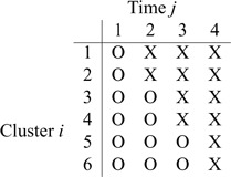In a standard SWD, is an integer, so that there are clusters randomized to each of intervention patterns. The following table illustrates a standard SWD with 6 clusters and 4 steps, where “X” represents the intervention periods and “O” represents standard of care. In this example, clusters are rolled over to the intervention at each step.

Unlike the pCRD, the SWD can incorporate time effects in design and analysis. We first derive a maximum likelihood method for power calculations for SWDs assuming no time effects in Section 2.1, and then extend the method to include time effects in Section 2.2.

2.1. Power calculations for the MLE of binary models: the case of no time effects

Suppose time effects do not need to be included in the model. This scenario is likely for trials of short duration, and when the effect of calendar time on the outcome is believed to be small. We consider a binary intervention, , and a binary outcome, , for participant in cluster at step . A GLMM (Breslow and Clayton, 1993) with the identity link is assumed,

(2.1)

where is the probability of the outcome in the comparison group, is the intervention effect, is the random cluster effect, and . By design, for all and . Following Hussey and Hughes (2007), the normal distribution for random effects, , is assumed, although in Section 3.3, we will explore the sensitivity of the methods to departures from this assumption.

When time effects are not included in the model, the outcomes for individuals in cluster can be re-organized as , with for all clusters. Correspondingly, the intervention indicators can be re-ordered as . Model (2.1) can then be rewritten as

(2.2)

The object of inference is the parameter , the risk difference, and the goal of the study is to test versus , where is the value of under the alternative hypothesis . We base power calculations on the Wald test for the MLE under its assumed asymptotic normal distribution. As usual, the asymptotic power is

(2.3)

where denotes the standard cumulative normal distribution, and is the th quantile of the standard normal distribution function with being the Type I error rate. The challenge here is to derive and compute the asymptotic variance of .

The full data likelihood for the model parameters from (2.2) is

and the log-likelihood is

(2.4)

where the limits of the integral over are imposed to ensure that the probabilities and , and is the indicator function. The factors and in the denominator normalize the integral to 1.

Because there are four possible configurations of and in this framework, (0,0), (0,1), (1,0) and (1,1), the study data for a single cluster can be written in terms of cell counts as shown below

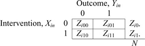
where is the number of individuals in cluster who receive the standard of care, is the number of individuals in cluster who receive the intervention, and the cluster size is . Both and are fixed by design, i.e., and , where is the number of steps in cluster randomly assigned to the intervention. We can rewrite log-likelihood (2.4) by utilizing as follows

(2.5)

Gauss-Legendre quadrature can be used to calculate this integral numerically.

Asymptotically, the variance of is given by

(2.6)

where is the expected Fisher information matrix. Let

(2.7)

By Leibniz’s rule for differentiation with integration, we obtain the derivatives of the log-likelihood function, as given in (S1.1)(S1.6) of the supplementary material available at Biostatistics online. Noting that

(2.8)

we calculate the expectations of the matrix elements in (2.8) with respect to . For example,

(2.9)

where is given by

(2.10)

and similarly for the expectation of other matrix elements in (2.8). Then, summation over all the clusters gives the expectation matrix (2.8) and is obtained from the appropriate element of its inverse. Hence, , the element of , is

(2.11)

where is the th row and th column of (2.8).

The formula (2.11) works well when the cluster size, , is not too big, say, less than several hundreds, as in many clinical trials. However, in public health interventions, may be greater than 1000 or even 10 000, as in the FIGO study in Section 4. The large leads to several numerical issues. First, when and are greater than 1000, the combinatorial numbers or will likely exceed the limit of machine precision, precluding exact binomial probability calculations. Second, when and are large, , , , or in (2.7) is small, sometimes below the limit of machine precision and will then be treated as zero, leading to inaccurate calculation. In these cases, we propose to use the normal approximation to the binomial, and in (2.7) as follows,

(2.12)

where , , , and .

Related work found that there was little effect on inference due to mis-specification of the random effects distribution under a logistic model for the binary outcome (Heagerty and Kurland, 2001; Neuhaus and others, 2011). Herein, we consider a gamma distribution for between-cluster random effects in model (2.1), similar to the one considered by Heagerty and Kurland (2001), i.e. , where with the density function , . The density function of is then given by with , with and , matching the first two moments of the assumed normal random effects distribution. Under this between-cluster random effect distribution, the log-likelihood (2.5) becomes

where is varied to obtain differently shaped distributions. Power based on different random effect distributions will be compared in Section 3.

When time effects are not included in the model, we note that the SWD is mathematically equivalent to a design where subjects in a cluster are randomly assigned to the intervention or standard of care with a cluster-specific allocation ratio (taking the trial in Section 4 as an example, 3:1 in the first three hospitals and 1:3 in the last three hospitals). However, this design may be difficult to implement in practice because subjects in the same cluster are assigned to different arms, as in an individually randomized clinical trial. Typically, in large scale efficacy trials, cluster-level randomization is required, logistically and because the intervention has cluster level components.

2.2. Power calculations for the MLE of binary models: the case for time effects

In this section, we extend the method of the previous section to the situation with time effects. Accordingly, a generalized linear mixed model (GLMM) with the identity link is defined as follows,

(2.13)

where is the time effect corresponding to step ( in , and for identifiability), and it is assumed that follows a normal distribution, . Since the probabilities in (2.13) are between 0 and 1, is not allowed to take any value as for a normal distribution. Thus, for an identity link, now follows a truncated normal distribution.

The full data likelihood for the model parameters , where , based on (2.13) is

(2.14)

The data for cluster at step can be summarized as , where and are the numbers of individuals having outcome 0 and 1, respectively, at step from cluster , and . With a slight abuse of notation, the full data log-likelihood function is

(2.15)

where follows a truncated normal distribution

GaussLegendre quadrature can be used for numerical integration. To simplify this formula, denote and . Then, the distribution of can be rewritten as

and must satisfy to make the distribution valid.

The asymptotic variance of the maximum likelihood estimator is,

where . With a slight abuse of notation, we define

By Leibniz’s rule, we obtain the derivatives as given in (S1.7)(S1.10) supplementary material available at Biostatistics online. The expectation with respect to can be calculated as

(2.16)

where is given by

(2.17)

Then the variance of in (2.3) is given by the corresponding component of estimated variance-covariance matrix .

When is large, numerical issues discussed in Section 2.1 are even more challenging. The normal approximation can be applied accordingly. Specifically, in (2.17) and in supplementary material available at Biostatistics online (S1.7)(S1.10) can be replaced with , where and . In addition, with time effects, the computations are even more intensive than that without time effects in the model. For example, consider the FIGO study (, ) in Section 4. When there are no time effects, we need to compute the derivatives in supplementary material available at Biostatistics online (S1.1)(S1.6) and the probability distribution in (2.10) for each possible combination of of cluster in (2.9). The number of possible combinations is for a single cluster. Without time effects in the model, the running time for the power calculation was about 85 s at our computational facility. However, when time effects are included in the model, we consider all possible combinations of of cluster in (2.16). In each cluster, there are combinations for which (S1.7)(S1.10) of the supplementary material available at Biostatistics online and (2.17) must be evaluated, leading to an estimated running time of over 1000 days at our high performance facility. We thus developed a partition method to approximate the power. At step in cluster , may take on values . We divide these numbers into equal partitions, and use their center values to represent these partitions. For example, suppose . The partitions are , , , and , centered at 112, 338, 563, and 788. We use these center values to approximate the expectation in (2.16) as

where the center values are about at and , for , with being the greatest integer function. To choose , we start from a small value, and then gradually increase until the difference between two consecutive calculated powers is less than 1%. In the FIGO study, starting from , and then , the power calculation stopped at . When , the calculation took about 0.6 hours, and when the running time was about 10.3 h. This partition method was very efficient, reducing the computational cost in this example from over 1000 days to 10.3 h.

3. Results

3.1. General observations

To explore the properties of the methods proposed in Section 2, we first studied the asymptotic power as a function of the risk difference and the number of steps.

To design a study, the assumed parameter values must be specified. The values of and can be determined by and . When time effects are included in the model, we assumed that the effects are linear across the time steps. If the change over the study duration is , . To illustrate the methods, we will consider and . The time effect for is almost negligible, and it is moderate for the other. The value of is determined by the intra-cluster correlation coefficient (ICC), , which measures the correlation between individuals in the same cluster. Following Hussey and Hughes (2007), in models (2.1) and (2.13), , where is the variance of cluster-specific random effects and the residual variance can be reasonably assumed to be , giving .

For an assumed baseline risk of outcome , we considered risk ratios in the range of 1.8 to 4.2, corresponding to risk differences . Figure 1 shows the power as a function of the risk difference, , for different numbers of steps and different ICCs. Here, the number of clusters is , the number of steps was varied as , and the ICC was set to 0.1 and 0.001 to represent large and small correlations, respectively. The cluster size was fixed at . In Figures 1(a) and (b), model (2.1) was used with no time effects. In Figure 1(a), when the ICC was large (), power became slightly lower as the number of steps increased. Because no time effect was included, the data become more unbalanced within a cluster between the intervention and control groups as the number of steps increases, and hence power decreases accordingly. When was small, it can be seen in Figure 1(b) that the effect of the number of steps on power decreases as the time effect diminishes, and the effect almost vanished as the ICC approached zero when there were no time effects. For example, for , when , there was 80% power to detect a risk difference of 0.0445, which corresponds to a risk ratio of 1.89; when , the minimum detectable risk difference was 0.0405, corresponding to a risk ratio of 1.81, for 80% power.

Fig. 1.

Power vs. risk difference , for and , with cluster size and baseline risk . For figures in the left column, ; while for figures in the right column, . There are no time effects () in the first row, very small time effects () in the second row, and moderate time effects () in the third row.

In Figure 1(c) and (d), although the time effects were very small (), model (2.13) was used for power calculations. Unlike what was seen in Figure 1(a) and (b), when time effects are included in the model, power increases with the number of steps. This may be because, in addition to the comparisons available between intervention and standard of care at the same step, the number of comparisons within cluster also increases as the number of steps increases. For , when there was 80% power to detect a risk difference of 0.092, corresponding to a risk ratio of 2.84; when , the risk difference with 80% power was 0.078, corresponding to a risk ratio of 2.56. The power in Figure 1(c) was much lower than the power in Figure 1(a), similar to the comparison between Figure 1(d) and (b). When time effects are anticipated to be negligible, the model without time effects is much more powerful.

In Figure 1(e) and (f), the time effects were moderate (). Specifically, for , when there was 80% power to detect a risk difference of 0.105 (risk ratio 3.1); when the minimum detectable risk difference with 80% power was 0.0885 (risk ratio 2.77). Again, the power increased with the number of steps.

In summary, when time effects are not included in the model, the power decreases with increasing number of steps given fixed cluster size and sample size; in contrast, when time effects are included in the model, the power increases with more time steps. When time effects are negligible, the model without time effects is much more powerful than the model with time effects.

3.2. Comparison of the power of SWDs with equal and unequal cluster sizes

So far we have assumed equal cluster sizes, . In practice, however, studies often have variable cluster sizes. Therefore, it is of interest to compare the efficiency of a SWD with equal cluster sizes to one with unequal cluster sizes. Previous work has considered the relative efficiency of unequal versus equal cluster sizes in the pCRD (van Breukelen and others, 2007; Candel and Van Breukelen, 2016), where it was found that power tends to decrease drastically as the variation in cluster sizes increases. We conducted numerical experiments to investigate the impact of variable cluster size on the power of the SWD. Two parameters need to be taken into account. One is the cluster size coefficient of variation (CV), defined as the square root of the variance of the cluster sizes divided by the mean cluster size; and the other is the intervention-control allocation ratio (TCR), defined as the ratio of study participants randomized to the intervention vs. those not. When the cluster sizes are equal, the cluster size CV is 0 and the TCR is 1. When the cluster sizes are unequal, the design then has a positive CV and a TCR that departs from 1, both of which could affect the study power.

The sample size of the numerical examples in this section was fixed at 480. Consider a SWD with clusters, a mean cluster size , and steps. We first fixed the TCR to be 1 and varied the cluster size CV. The cluster size was 30 for each cluster in the equal cluster size design, while for the unequal cluster size design, we randomly assigned 240 individuals to the first eight clusters using a multinomial distribution with , and then another 240 individuals to the second eight clusters using a multinomial distribution with . Thus, the TCR was still 1 although the cluster size CV = 2.0. For baseline risk and , the power curves versus risk differences are displayed in Figure S1(a) of the supplementary material available at Biostatistics online without time effects, in Figure S1(c) of the supplementary material available at Biostatistics online with very small time effects, and in Figure S1(e) of the supplementary material available at Biostatistics online with moderate time effects. We can see that there is virtually no difference between these curves. Overall, with TCR = 1, power was very similar between the two designs.

We next varied the TCR from 1 to 0.7 by setting the total sample size of the first eight clusters to 96 and the total sample size of the second eight clusters to 384, or, equivalently, by setting the cluster size of the first eight clusters to 12, and to 48 for the second eight clusters, which produced a cluster size CV = 0.6. In addition, we created another design by randomly assigning 96 individuals to the first eight clusters using a multinomial distribution with . We then assigned another 384 individuals to the second eight clusters using a multinomial distribution with , to obtain a TCR of 0.7 and a cluster size CV of 2.0. We then changed TCR to 1.5 by setting the total sample size of the first eight clusters to be 384 and the total sample size of the second eight clusters to be 96. We assigned subjects to the clusters as previously, so the cluster size CVs were still 0.6 and 2.0, respectively. We plotted the power curves for these two TCRs in red and in blue, respectively, along with the plots explored previously in Figure S1(a) of the supplementary material available at Biostatistics online without time effects, in Figure S1(c) of the supplementary material available at Biostatistics online with very small time effects, and in Figure S1(e) of the supplementary material available at Biostatistics online with moderate time effects, in the supplementary material. We can see that the two power curves with the same TCR were very close, although they had quite different cluster size CVs, again verifying the previous observation that SWD power is insensitive to different cluster size CVs for a fixed TCR.

When there were no time effects as in Figure S1(a) of the supplementary material available at Biostatistics online, the effect of TCR on power is small. However, for the model with time effects, TCR had a marked impact on power (Figures S1(c) and (e) of the supplementary material available at Biostatistics online). When TCR=1, i.e. half the participants are randomized to the intervention, the SWD was the most efficient. To further investigate the role of TCR on SWD power, we repeated the above numerical study with a baseline risk (Figures S1(b), (d) and (f) of the supplementary material available at Biostatistics online). Similar patterns were observed.

Overall, the findings from these numerical studies suggest that the effect of cluster size CV on power in the SWD is, in general, small, for a fixed TCR. Without time effects, there is little effect of TCR on power, while with time effects, TCR has a much greater effect. However, when a SWD is well randomized, the TCR will not depart too much from 1. It is reasonable to conclude that the power of the SWD is robust to variable cluster size.

3.3. Comparison of power with different assumed random effect distributions

Now, we consider the gamma random effect distribution discussed in Section 2.1, with and , to incorporate a wide range of shapes. The density plots of the gamma distributions considered are given in Figure S2 of the supplementary material available at Biostatistics online. The gamma distribution with looks very different from the standard normal distribution, while the shape of the density function is closer to normal with .

In Figure 2, assuming a SWD with , , and a cluster size , we show power curves with different distributions of the cluster random effects. There were no time effects in Figure 2(a) and (b). When the was small (), in Figure 2(a), the power curves for the three distributions were nearly identical. In Figure 2(b), when was substantially larger, a bigger difference between these three power curves was observed, although they were still quite close. When the time effects were very small (Figure 2(c) and (d) ) or moderate (Figure 2(e) and (f)) the power curves from different random effects distributions were also very similar. These observations suggest that, for random effects distributions with the same mean and variance but different higher order moments, the distribution of the cluster random effects has little effect on the power of a SWD, as has previously reported (Heagerty and Kurland, 2001; Neuhaus and others, 2011).

Fig. 2.

Power vs. the risk difference for different cluster random effect distributions, with baseline risk , number of steps , number of clusters , and cluster size . For figures in the left column, ; while for figures in the right column, . There are no time effects () in the first row, very small time effects () in the second row, and moderate time effects () in the third row.

3.4. Comparison to the Hussey and Hughes (2007) method

Next, we compared the efficiency of the MLE estimator for a SWD to that of the WLS estimator of Hussey and Hughes (2007). First, we assumed no time effects. In Hussey and Hughes (2007), the variance of the WLS estimator based on model (2.1) is

(3.1)

where , with an indicator of the intervention status randomly assigned to cluster at time , , and is the ICC. This simplified expression was given by Zhou and others (2017). An extra factor of was omitted from equation (9) in Hussey and Hughes (2007) but is included in the numerator of (3.1) (Liao and others, 2015).

In Figure 3(a) and (b), we compared the relative variances (ARE) of and using (3.1) for models without time effects, over different values of the baseline risk , and the risk difference , in a SWD of eight clusters with 90 subjects in each cluster, five steps, and . The variance of was over-estimated (i.e. the ARE was greater than 1) for some values of and , and under-estimated for others.

Fig. 3.

ARE of relative to . Figures in the left column show ARE vs. baseline risk with the risk difference ; Figures in the right column show ARE vs. risk difference with the baseline risk . There are no time effects () in the first row, very small time effects in the second row (), and moderate time effects in the third row (). The number of clusters , the number of steps , the cluster size , and .

When there are time effects, the variance of the WLS estimator is given by

(3.2)

where . Again, this simplified expression was given by Zhou and others (2017). Figure 3(c)–(f) compared the relative variances (ARE) of and for model (2.13) with very small or moderate time effects. As with no time effects, the variance of was over-estimated for some values of and , and under-estimated for others.

Since Hussey and Hughes (2007) assumed that the within-cluster variance was , the variance in (3.1) and (3.2) does not depend on the underlying risk difference , while the variance of the MLE does, as is the case with binomial data in general. This approximation likely leads to inaccuracies in the calculation of . In addition, the WLS approach assumes that is known, which will not be true in practice, or at least, that its estimate is uncorrelated with the estimate of the mean function parameters as would be the case in a linear model under normality assumptions. In contrast, the MLE takes into account the estimation of in deriving the variance, as well as its correlation with , , and , and thus it will be a more honest assessment of the power although it may be less efficient because it estimates an additional parameter. Thus, our findings suggest that power calculations for the SWD should be based on the variance of the MLE or the variance of another consistent estimator which accounts for these key features of binomially distributed outcome data.

3.5. Comparison of the SWD to the parallel cluster randomized design

It is also of interest to compare the SWD to the pCRD, in which, at the start of the study, typically half of the clusters are randomized to the intervention group and half to the control group. As given by Donner and Klar (2000),

(3.3)

Firstly, consider the SWD without time effects, as shown in the left column of Figure 4. Figure 4(a) displays the power of the SWD and pCRD as a function of the number of clusters, varying from 8 to 80, with , , and . The power curves for the SWD and pCRD as a function of the risk difference, which varies from 0 to 0.2, are shown in Figure 4(c), with fixed baseline risk and for several values of , the number of clusters. We can see that the SWD has greater power than the pCRD in all scenarios explored. Figure 4(e) and Figure S3(a) of the supplementary material available at Biostatistics online show the power curves for the SWD and pCRD as a function of the ICC for different numbers of clusters and different baseline risks. We can see that the power of the pCRD decreases quickly as the ICC increases, while the power of SWD barely changed either in Figure 4(e) for a small baseline risk (rare outcome), or in Figure S3(a) of the supplementary material available at Biostatistics online for a big baseline risk (common outcome). Also, the rate of the change of the power function with increasing ICC was very similar in the SWD for different numbers of clusters as can be seen in Figure 4(a). But for the pCRD, the power declined even faster with increasing ICC as the number of clusters increased. In Section S3 of the supplementary material available at Biostatistics online, we prove that the power of the SWD based on the MLE variance (2.11) is always bigger than that of the pCRD based on the variance (3.3), emphasizing the efficiency advantage of the SWD over the pCRD, when there are no time effects included in the model. Intuitively, this point seems obvious. There are only between-cluster comparisons in the pCRD, while there are, in addition, within-cluster comparisons in the SWD (Zhou and others, 2017).

Fig. 4.

Comparison between SWD and pCRD. There are no time effects in the model for figures in the left column, and moderate time effects in the model for figures in the right column. (a) and (b) power vs. the number of clusters, with baseline risk , the risk difference , the cluster size , and ; (c) and (d) power vs. the risk difference , with baseline risk , the cluster size , the , and the number of steps ; (e) and (f) power vs. ICC, for different baseline risks , where the risk difference , the cluster size , and the number of steps .

Next, we considered the comparison with the pCRD when time effects were included in the model for the SWD. Suppose that for the pCRD, individuals at different time steps are well balanced in each cluster. That is, the formula (3.3) is still appropriate, since the time step is not a confounder in the pCRD. The comparison between SWD and pCRD is shown in the right column of Figure 4, when the time effects are moderate (). Figure 4(b) and (d) display the power of the SWD and pCRD as a function of the number of clusters, and as a function of the risk difference, respectively, with . The SWD has lower power than the pCRD, since the SWD has to estimate more parameters, , in the model. However, as the ICC increases, as shown in Figure 4(f) and Figure S3(b) of the supplementary material available at Biostatistics online, the SWD still provides better power. As seen previously, the power of SWD barely changed as the ICC increases.

4. Illustrative example

In collaboration with the International Federation of Gynaecology and Obstetrics (FIGO) and the Association of Gynaecologists and Obstetricians of Tanzania (AGOTA), the Harvard T.H. Chan School of Public Health (HSPH) designed a study of the impact and performance of a postpartum IUD (PPIUD) intervention in Tanzania (Canning and others, 2016). The FIGO/AGOTA intervention will take place over 1-year (9 months in the first group of three hospitals and 3 months in the second group of three hospitals). The study design is illustrated below, with X = PPIUD intervention and O = standard of care.

Time (months)		1–3	4–6	7–9	10–12
Group 1	Hospital 1	O	X	X	X
	2	O	X	X	X
	3	O	X	X	X
Group 2	4	O	O	O	X
	5	O	O	O	X
	6	O	O	O	X

In this SWD, there are clusters (hospitals) and steps, each 3 months long. Although this is not a standard SWD, our method still applies, using the treatment assignments in the above table. The primary outcome is the pregnancy rate within 18 months of the index birth. Based on data from the 2010 Tanzania Demographic and Health Survey, the 18-month new pregnancy rate was 18.1% and the ICC was 0.022. Approximately 300 women per month will join the study in each of the six participating Tanzanian hospitals, yielding per cluster per step. Hence, each cluster size is and the total sample size is . As we discussed in Sections 2.1 and 2.2, this cluster size is very large, requiring the use of the normal approximation for the model without time effects, and in addition the partition method for the model with time effects.

For illustrative purposes, we first considered a smaller cluster size scenario, namely and cluster size . With this scenario, we were able to compare the power obtained with the exact calculations to that with the numerical approximations, to assess their accuracy. When there were no time effects, the exact calculations of (2.7) produced a power of 62.3% for detecting a risk ratio of 0.8, corresponding to a decrease in the 18 month pregnancy rate, compared with 62.0% for the normal approximation; the power was 19.7% for detecting a risk ratio of 0.9, corresponding to a decrease, for both the exact calculation and normal approximation methods. When the time effect over one year study period is assumed to correspond to a 10% decrease in the baseline risk (), the exact calculation method yielded a power of 28.4% for a risk ratio of 0.8, and 10.3% for a risk ratio of 0.9. For the normal approximation and partition method with a maximum of 32, the calculated powers were 28.3% and 10.4% for risk ratios of 0.8 and 0.9, respectively. These results suggest excellent performance for the numerical techniques we have proposed.

When the cluster size was set to 3600 as in the actual study, computational limitations required the use of the normal approximation and the partition method for power calculations. We considered possible time effects over the one-year study period: (i) no time effects (); (ii) negligible time effects (); (iii) 5% decrease of the baseline risk (); (iv) 10% decrease of the baseline risk (). We also compared the power based on the MLE variance to that based on the WLS variance. The results are given in Table 1. When there were no time effects, the ARE of MLE to Hussey and Hughes’ WLS method is 1.275 for detecting a risk ratio of 0.8 and 1.207 for detecting a risk ratio of 0.9, indicating that if Hussey and Hughes’ method were used for power calculations, the study budget/sample size would be nearly 25% greater than necessary. When there were time effects, we used the partition method. The procedure for choosing is given in Table S1 of the supplementary material available at Biostatistics online. As shown in Table 1, the power was roughly insensitive to the time effects, and was higher in our approach than the WLS method. Notice that when the time effects are negligible, the power was much lower than that without time effects when the intervention effect was , corresponding to a risk ratio of 0.9.

Table 1.

Power of the PPIUD study in Tanzania, for several plausible time effects and hypothesized risk ratios

		Time effects
		Risk ratio			Risk ratio			Risk ratio			Risk ratio
		0.8	0.9		0.8	0.9		0.8	0.9		0.8	0.9
Power	MLE	1.000	0.908		0.976	0.480		0.981	0.494		0.984	0.506
	H&H	1.000	0.850		0.935	0.412		0.935	0.412		0.935	0.412
ARE		1.275	1.207		1.288	1.208		1.348	1.254		1.387	1.291

5. Discussion

Little statistical theory for SWDs for binary outcome data has been developed to date—this article fills that gap. In this article, we developed a numerical method calculating the asymptotic power for a SWD with a binary outcome. Numerical integration over the distribution of the unobserved random cluster effects is required. By doing so, we were able to appropriately account for the binary nature of the outcome data using maximum likelihood theory. We showed through several design scenarios that the resulting power did not agree with that given by Hussey and Hughes (2007) using their closed form approximation. There are two sources of discrepancies. One is that the Hussey and Hughes estimator incorrectly assumes that the variance of the outcome is constant, since the variance of a binomial distribution is related to its mean. Thus, the Hussey and Hughes estimator could be either over- or under-powered. The other is that the variance, , of between-cluster random effects is assumed known in Hussey and Hughes (2007). This assumption is invalid in practice, and likely results, all other things being equal, in an over-estimation of the power. The maximum likelihood method developed in this article does not make either of these assumptions and, in addition, was found to be robust against different random effect distributions.

In this article, we have developed power calculations for binary outcomes modeled either as a function of time or not. A natural question is which model should be used in practice for study design. When we are quite sure about the existence of time effects, the model with time effects should be used. However, it is often the case that the time effects are believed to be small or negligible during the study period, if they exist at all, particularly with studies of short duration. A recent review by Martin and others (2016) found that, among 45 studies which reported a sample size calculation, 36% allowed for time effects, while 31% did not. If time effects are considered at the design stage, a much larger sample size will be required, as seen in Sections 3 and 4. However, if we assume that there are no time effects at the design stage, and a time trend is found, the estimated intervention effect will be biased unless it is adjusted for time in the analysis. Adjusting for this unanticipated time trend at the analysis phase will likely lead to an underpowered study. Subject matter considerations, prior knowledge, and common sense will have to guide these decisions.

In this work, we considered a random intercept in models (2.1) and (2.13). Recently, others have proposed models that include random time effects (Hughes and others, 2015) and random treatment effects (Hooper and others, 2016) for continuous outcomes. Theoretically, it is straightforward to extend our method to include such variation with binary outcomes. To do so, would require developing accurate and efficient numerical methods for multiple integration, a challenging task. It will be of great interest to investigate these extensions in future work.

Following the seminal work of Hussey and Hughes (2007), in this article, we considered the identity link so that the intervention effect is given on the risk difference scale. In future work, we will consider extensions to the log link and logistic link, where the parameter of interest is the risk ratio and odds ratio. User-friendly software based on our method is available online at https://github.com/xinzhoubiostat/swdpower.

Supplementary Material

BIOSTS_21_1_102_s7

Supplementary Data

Supplementary material

Supplementary material is available at http://biostatistics.oxfordjournals.org.

Funding

National Institute of Environmental Health Sciences [DP1ES025459]; National Institute of Allergy and Infectious Diseases [R01AI112339]; Food and Drug Administration [U01FD00493].

References

- Breslow N. E. and Clayton D. G. (1993). Approximate inference in generalized linear mixed models. Journal of the American Statistical Association 88, 9–25. [Google Scholar]
- Brown C. A. and Lilford R. J. (2006). The stepped wedge trial design: a systematic review. BMC Medical Research Methodology 6,54. [DOI] [PMC free article] [PubMed] [Google Scholar]
- Candel M. J. J. M. and Van Breukelen G. J. P. (2016). Repairing the efficiency loss due to varying cluster sizes in two-level two-armed randomized trials with heterogeneous clustering. Statistics in Medicine 35, 2000–2015. [DOI] [PubMed] [Google Scholar]
- Canning D., Shah I., Pearson E., Pradhan E., Karra M., Senderowicz L., Barnighausen T., Spiegelman D. and Langer A. (2016). Institutionalizing postpartum intrauterine device (PPIUD) services in sri lanka, tanzania, and nepal: study protocol for a longitudinal cluster-randomized stepped wedge trial. BMC Pregnancy and Childbirth 16, 362. [DOI] [PMC free article] [PubMed] [Google Scholar]
- Donner A. and Klar N. (2000). Design and Analysis of Cluster Randomization Trials in Health Research. London: Arnold. [Google Scholar]
- Hayes R. J. and Moulton L. H. (2009). Cluster Randomised Trials. Boca Raton, FL: Chapman and Hall/CRC. [Google Scholar]
- Heagerty P. J. and Kurland B. F. (2001). Misspecified maximum likelihood estimates and generalised linear mixed models. Biometrika 88, 973–985. [Google Scholar]
- Hemming K., Haines T. P., Chilton P. J., Girling A. J. and Lilford R. J. (2015). The stepped wedge cluster randomised trial: rationale, design, analysis, and reporting. BMJ 350, h391. [DOI] [PubMed] [Google Scholar]
- Hemming K. and Taljaard M. (2016). Sample size calculations for stepped wedge and cluster randomised trials: a unified approach. Journal of Clinical Epidemiology. 69, 137–146. [DOI] [PMC free article] [PubMed] [Google Scholar]
- Hooper R., Teerenstra S., De Hoop E. and Eldridge S. (2016). Sample size calculation for stepped wedge and other longitudinal cluster randomised trials. Statistics in Medicine 35, 4718–4728. [DOI] [PubMed] [Google Scholar]
- Hughes J. P., Granston T. S. and Heagerty P. J. (2015). Current issues in the design and analysis of stepped wedge trials. Contemporary Clinical Trials 45, 55–60. [DOI] [PMC free article] [PubMed] [Google Scholar]
- Hussey M. A. and Hughes J. P. (2007). Design and analysis of stepped wedge cluster randomized trials. Contemporary Clinical Trials 28, 182–191. [DOI] [PubMed] [Google Scholar]
- Liao X., Zhou X. and Spiegelman D. (2015). A note on “Design and analysis of stepped wedge cluster randomized trials”. Contemporary Clinical Trials 45, 338–339. [DOI] [PMC free article] [PubMed] [Google Scholar]
- Martin J., Taljaard M., Girling A. and Hemming K. (2016). Systematic review finds major deficiencies in sample size methodology and reporting for stepped-wedge cluster randomised trials. BMJ Open 6, e010166. [DOI] [PMC free article] [PubMed] [Google Scholar]
- Neuhaus J. M., McCulloch C. E. and Boylan R. (2011). A note on Type II error under random effects misspecification in generalized linear mixed models. Biometrics 67, 654–660. [DOI] [PMC free article] [PubMed] [Google Scholar]
- Van Breukelen G. J. P., Candel M. J. J. M. and Berger M. P. F. (2007). Relative efficiency of unequal versus equal cluster sizes in cluster randomized and multicentre trials. Statistics in Medicine 26, 2589–2603. [DOI] [PubMed] [Google Scholar]
- Zhou X., Liao X. and Spiegelman D. (2017). “Cross-sectional” stepped wedge designs always reduce the required sample size when there is no effect of time. Journal of Clinical Epidemiology 83, 108–109. [DOI] [PMC free article] [PubMed] [Google Scholar]
Associated Data
This section collects any data citations, data availability statements, or supplementary materials included in this article.
Supplementary Materials