

Summary
Genome-wide mapping of chromatin interactions at high-resolution remains experimentally and computationally challenging. Here we used a low-input “easy Hi-C” protocol to map the 3D genome architecture in human neurogenesis and brain tissues, and also demonstrated that a rigorous Hi-C bias-correction pipeline (HiCorr) can significantly improve the sensitivity and robustness of Hi-C loop identification at sub-TAD level, especially the enhancer-promoter (E-P) interactions. We used HiCorr to compare the high-resolution maps of chromatin interactions from 10 tissue- or cell-types with a focus on neurogenesis and brain tissues. We found that dynamic chromatin loops are better hallmarks for cellular differentiation than compartment switching. HiCorr allowed direct observation of cell type- and differentiation-specific E-P aggregates spanning large neighborhoods, suggesting a mechanism that stabilizes enhancer contacts during development. Interestingly, we concluded that Hi-C loop outperforms eQTL in explaining neurological GWAS results, revealing a unique value of high-resolution 3D genome maps in elucidating the disease etiology.
Keywords: Hi-C, eHi-C, HiCorr, bias correction, chromatin loop, enhancer-promoter interaction, transcription regulation, neurogenesis, GWAS
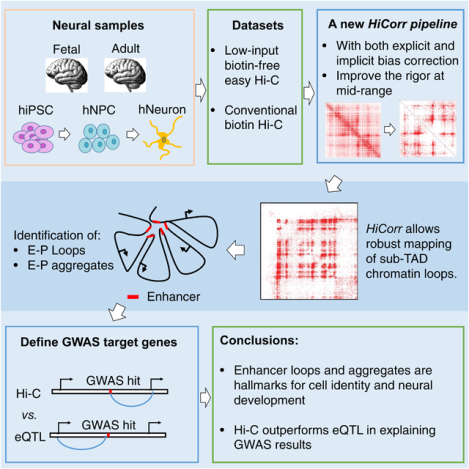
Graphical Abstract
eTOC Blurb
Lu et al. developed a rigorous Hi-C bias-correction pipeline to significantly improve the robustness of high-resolution chromatin interaction maps. With a new low-input “easy Hi-C” protocol, they mapped chromatin interactions in neural samples, defined cell type-specific enhancer loops and aggregates, and concluded that Hi-C outperforms eQTL in explaining GWAS results.
Introduction
Hi-C has transformed our understanding of mammalian genome organization (Denker and de Laat, 2016; Lieberman-Aiden et al., 2009). In the past decade, with increasing sequencing depth, a hierarchy of 3D genome structures, such as compartment A/B (Lieberman-Aiden et al., 2009), topological domains or topological associated domains (TADs) (Dixon et al., 2012; Nora et al., 2012) were revealed. More recently, kilobase resolution Hi-C analysis was achieved with sequencing depth at billion-read scale (Jin et al., 2013; Rao et al., 2014). At this resolution, it is possible to discern specific chromatin loops between cis-regulatory elements. The information inherent in the 3D genome, especially chromatin loops, is critical for understanding the genetics of complex diseases (de Wit et al., 2013; Jin et al., 2013; Kagey et al., 2010; Phillips-Cremins et al., 2013), such as the GWAS of cognitive traits and psychiatric disorders (Won et al., 2016; Wray et al., 2018).
However, kilobase-resolution Hi-C analysis is challenging both experimentally and computationally, especially when the amount of starting material is small. Experimentally, it is important to develop low-input Hi-C protocols that can deliver high quality libraries for ultra-deep sequencing. Computationally, mapping chromatin interactions with Hi-C at high-resolution suffers from the difficulty to correct the data biases, which leads to the low reproducibility or coverage in loop calling (Forcato et al., 2017). For example, the commonly used genome-wide loop caller HICCUPS yields ~104 CTCF loops (Rao et al., 2014) that only explain a small number of GWAS hits; Several recent Hi-C studies called SNP/gene interactions with locus-focused algorithms (Rajarajan et al., 2018; Wang et al., 2018; Won et al., 2016), but those algorithms are not suitable for unbiased genome-wide loop calling and usually have strong biases towards selected loci and a high false positive rate. Alternatively, other studies using targeted capture Hi-C, ChIA-PET, HiChIP, etc. (Fang et al., 2016; Javierre et al., 2016; Mifsud et al., 2015; Mumbach et al., 2017; Schoenfelder et al., 2015a; Zhang et al., 2013) reported many more E-P interactions, even though those methods are incomprehensive, biased due to target selection, and sometimes require even more biomaterials than Hi-C. Currently there is not a consensus whether Hi-C is a viable option to map E-P loops at sub-TAD level for transcription regulation and human disease studies.
To address these challenges, we developed a new genome-wide Hi-C bias-correction pipeline that substantially improved the mapping of sub-TAD chromatin loops at fragment resolution. We also developed a genome-wide all-to-all version of 4C (Simonis et al., 2006) protocol named “easy Hi-C” (eHi-C), which yields high complexity Hi-C libraries with 50–100K cells as the starting material. With these new toolsets, we mapped chromatin loops in 10 (e)Hi-C datasets and revealed new insights into the transcriptional regulation and the genetics of human diseases.
Results
Design and performance of eHi-C
In Hi-C, 5’ overhangs are created after restrictive DNA digestion (e.g. with HindIII) so that ligation junctions can be labeled with biotinylated nucleotides and eventually enriched in a pull-down step with streptavidin beads. However, this biotin-dependent strategy has intrinsic limitations that prevent the use of Hi-C if only low cell inputs are possible, because the efficiency of biotin incorporation is low (Belton et al., 2012), and the recovery rate of biotin-labeled DNA from the pull-down procedure can be variable.
We therefore developed eHi-C to circumvent the limitations of Hi-C by using a biotin-free strategy to enrich ligation products (Figure 1A). The eHi-C protocol is essentially a genome-wide “all-to-all” version of 4C (Simonis et al., 2006), and only involves a series of enzymatic reactions. eHi-C is also closely similar to ELP, another biotin-free genome-wide method developed several years ago for fission yeast 3D genome analysis (Tanizawa et al., 2010). However, ELP does not remove contamination from several species of non-junction DNA, and < 4% of ELP reads represent proximity ligation events (Tanizawa et al., 2010). Our eHi-C protocol has several key improvements, which allows the generation of high-yield libraries from small amount of input tissues (Figure S1A–J, more discussion in STAR Methods). We tested low-input eHi-C with 0.1 million IMR90 cells and found that the resulting DNA libraries had an equivalent complexity as published conventional Hi-C libraries generated with 10 million IMR90 cells; the yield of cis-contacts from eHi-C libraries is also better than most of the published HindIII-based Hi-C libraries (Table S1 and Figure S1G–H). At low resolution, the contact heatmaps from Hi-C and eHi-C data are nearly identical showing the same compartment A/B (Lieberman-Aiden et al., 2009) and TAD (Dixon et al., 2012; Nora et al., 2012) structures (Figure 1B–C). The eHi-C method also demonstrated near perfect reproducibility with different sequencing depth, and between biological replicates in the compartment and TAD analyses (Figure S1I–J). Finally, since eHi-C has a distinct error source and bias structure from conventional Hi-C due to protocol differences (STAR Methods and Figure S1K–P), we have adjusted our data filtering and normalization method to unify the high-resolution analysis of both Hi-C and eHi-C data (see later discussion).
Figure 1. Mapping 3D genome with eHi-C.
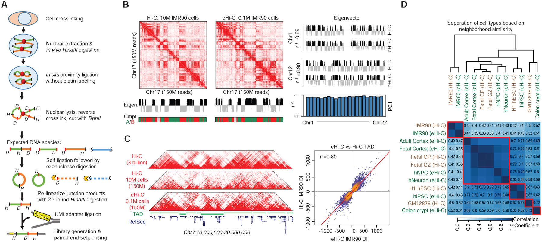
A, The scheme of eHi-C. B, Heatmaps show the contact matrices (Chr17) from Hi-C and eHi-C at 250kb resolution. The eigenvectors from Hi-C and eHi-C were very similar, leading to the same compartment A/B assignment. The comparison of eigenvectors between Hi-C and eHi-C in two other chromosomes are shown in the right panel. Histogram listed the r2 values of all chromosomes when comparing eigenvectors between eHi-C and Hi-C data. C, Heatmaps of contact matrices from Hi-C and eHi-C at 40kb resolution. The top track is drawn using a published IMR90 Hi-C dataset with ~3 billion reads. A track of TAD structures is plotted in green. On the right is a scatter plot comparing the directionality indexes (DI). The +/− sign of DI is used to determine TAD boundary. Very few bins change their signs of DI, indicating consistent TAD boundaries between Hi-C and eHi-C. D. Heatmap showing the similarity between 5 Hi-C and 7 eHi-C datasets (including a low-depth IMR90 eHi-C dataset) at compartment level. The correlation coefficient is computed by comparing the correlation matrices from different samples.
Billion-read scale 3D genome datasets in 10 cell- or tissue- types
Theoretically, the best Hi-C analysis resolution is determined by the restrictive endonuclease used (~2 kb for 6-base cutters, and ~200 bp for 4-base cutters). However, due to the lack of sequencing depth, high-resolution analysis at kilobase-scale is only achievable within 1–2 Mb. We estimated that for 6-base cutters, ~200 million mid-range (within 2 Mb) cis-contacts are required for fragment-level analysis (5–10 kb resolution); usually this translates into ~ 1–2 billion total non-redundant read pairs (STAR Methods).
We have successfully performed eHi-C in multiple cell- and tissue types. Five of our eHi-C datasets meet this sequencing depth requirement, including human induced pluripotent stem cells (hiPSCs), derived human neural progenitor cells (hNPCs), human neurons (hNeurons) and two postmortem brain tissues (fetal cerebrum and adult anterior temporal cortex) (Table S1). The hNPCs and hNeurons were derived from hiPSCs using a previous established forebrain neuron-specific differentiation protocol (Chiang et al., 2011; Wen et al., 2014) (Figure S2A–E). We also generated or obtained billion read-scale conventional Hi-C data for the H1 human embryonic stem cell (hESC), IMR90 (skin fibroblast) (Jin et al., 2013), GM12878 (B-Lymphocyte line) (Rao et al., 2014; Selvaraj et al., 2013), and two developing human cerebral cortex samples (cortical plate, fetal CP; and germinal zone, fetal GZ) (Won et al., 2016) (Table S1 and S2). Altogether, we have sufficient sequencing depth for fragment-resolution analysis in 10 tissue- or cell- types.
Genome compartmentalization is known to associate with cell identity and gene regulation (Bickmore and van Steensel, 2013; Dekker and Mirny, 2016; Dixon et al., 2015; Lieberman-Aiden et al., 2009). We therefore performed compartment analysis to examine the overall cell-specificity of the Hi-C and eHi-C libraries. The analysis defines compartment A/B with the first principal component values (PC1) (Lieberman-Aiden et al., 2009), which represents the euchromatin/heterochromatin neighborhoods (Figure S2F). As expected, hiPSCs and hESCs have very similar correlation matrices despite the difference in the Hi-C protocol; neural differentiation causes significant changes of genome compartments, consistent with previous reports (Beagan et al., 2016; Krijger et al., 2016) (Figure S2F). Clustering analysis further showed a highly tissue- or cell-type specific genome compartmentalization (Figure 1D). Notably, all brain/neuron related samples clustered together, and the three fetal brain samples (two Hi-C and one eHi-C) formed the tightest sub-cluster (Figure 1D). These results demonstrate the consistency between eHi-C and Hi-C at the low resolution.
HiCorr improves the rigor of Hi-C bias-correction at high-resolution
Identifying chromatin loops, especially the E-P interactions at the sub-TAD level, remains a major bioinformatic challenge in Hi-C analysis, as it is increasingly difficult to correct biases when the resolution increases to single fragment level (Forcato et al., 2017). We previously developed a method to explicitly correct fragment size, distance, GC content and mappability biases, and to estimate the expected frequency between any two fragments (Jin et al., 2013; Yaffe and Tanay, 2011). Using joint function, this method can correct the interaction effects between parameters (e.g. the interaction between fragment size and distance). However, this explicit method does not correct biases from unknown sources. Alternative strategies, such as VC normalization (Lieberman-Aiden et al., 2009), ICE (Imakaev et al., 2012) and Knight-Ruiz (KR) matrix-balancing algorithms (Rao et al., 2014), correct both known and unknown biases by normalizing a “visibility” factor (usually the total read counts) for each locus, with or without iterations. However, these implicit methods assume all biases are hidden in the visibility factor, and the visibility biases are “factorizable” (i.e. the visibility between different loci are independent). These assumptions are questionable at high-resolution within short to mid-ranges (more discussion in STAR Methods). For example, implicit methods do not correct the biases from distance or from the size selection of ligation products during Hi-C or eHi-C library preparation (Figure S1O).
We developed a new strategy named HiCorr that corrects the implicit “visibility” factor after normalizing all aforementioned known biases, that consequently has the advantages of both explicit and implicit methods. HiCorr estimates expected values for every fragment pair and uses observed / expected ratios to determine chromatin interactions (Figure S3A, STAR Methods). Importantly, we computed the “visibility” only using the trans- reads. This is because normalizing cis- visibility has the risk of over-correction since many cis- reads come from chromatin loops (Figure 2A): we found that cis- visibility is higher at histone marked loci and repetitive elements. The latter is possibly due to the widespread contribution of transposable elements to the transcriptional regulatory sequences in the mammalian genome (Sundaram et al., 2014) (Figure 2B–D). From the HiCorr-corrected ratio heatmaps, we can directly observe discrete chromatin loops without the interference from local DNA packaging signal along the diagonal. Compared to other normalization methods, HiCorr significantly improves the sharpness of Hi-C heatmaps, highlights the sub-TAD chromatin interactions, and does not have the over-correction problem at the short range (Figure 2E, compare the last column with other columns, more examples in Figure S3C). Notably, the implicit “visibility” correction step in HiCorr allows proper normalization of large copy number variants, which is difficult for explicit bias-correction strategy to correct, as exemplified by Hi-C data in the 22q11.2 heterozygous deletion cells (Zhang et al., 2018) (Figure S3B).
Figure 2. HiCorr improves the rigor of Hi-C bias-correction.
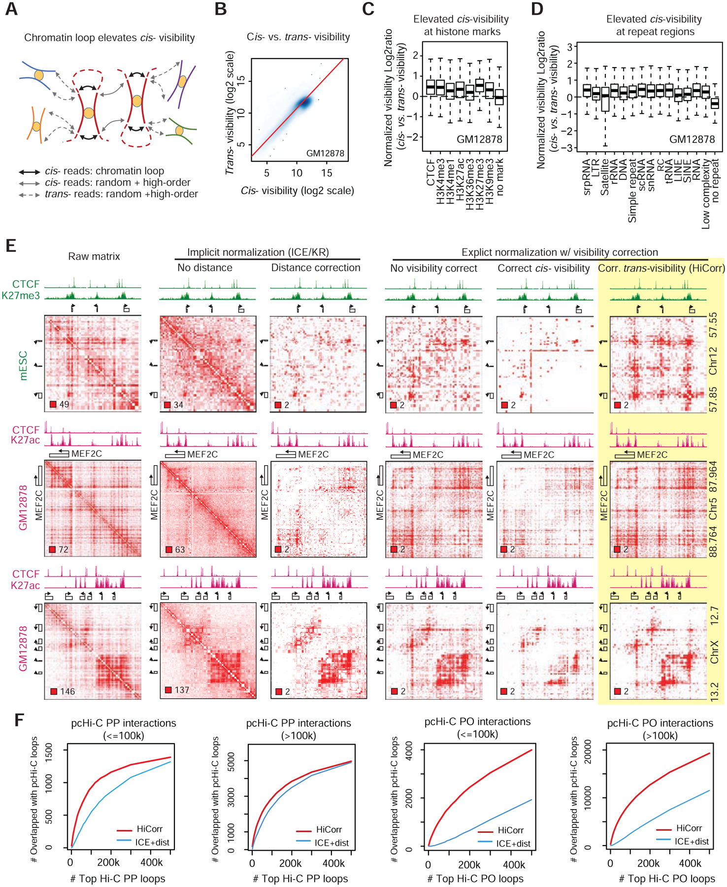
A, Chromatin loops contributes to cis but not trans Hi-C reads, leading to an elevated cis/trans visibility ratio. B, Scatter plot of all fragments in GM12878 Hi-C data showing a skew towards higher cis- than trans- visibility. C-D, Epigenetically marked regions and repeat elements have a higher cis/trans visibility ratio. E, Comparing the results of different visibility correction methods. The number in the lower left corner indicates color scale. For example, the color box of “2” in the ratio heatmaps indicates that any contact with O/E > 2 will be shown in dark red; contacts with 1< O/E < 2 will be in light red; white pixels in the heatmaps are O/E < 1. F. Comparison between HiCorr and ICE in capturing promoter-centered interactions from pcHi-C data in GM12878 cells. Note that for ICE curves, we performed ICE normalization followed by distance-correction. The promoter-center interactions from pcHi-C are divided into four groups based on distance (short- or long-range) and the type of interactions (promoter-promoter or promoter-other). The plots showing the number of recovered pcHi-C interactions when the same number of total loop pixels were called from HiCorr- or ICE-corrected contact heatmaps. Up to 500K total loop pixels were tested in these plots.
HiCorr reveals sub-TAD E-P interactions and aggregates robustly
Since HiCorr outputs ratio matrices representing the fold enrichment of Hi-C signal, we can conveniently call red pixels from the HiCorr-corrected heatmaps as chromatin interactions. In this study, we use a simple method calling pixels with ratio greater than 2 and p value better than 0.001 as chromatin interactions, after excluding low-coverage pixels (STAR Methods). This intuitive pixel-level method does not make prior assumptions about the distance, shape, size, or density of chromatin loops. We found that with sequencing depth at 150~200 million mid-range contacts, our method called 60~150K loop pixels with a high reproducibility at 40~60% between biological replicates, which is a significant improvement compared to the metrics of existing methods according to (Forcato et al., 2017) (Figure S4, more discussion in STAR Methods). Inadequate sequencing depth appears to be the major reason for non-reproduced loops, and most non-reproduced pixels can be recovered with lower threshold (Figure S4A–D). We therefore always preferred to call loop pixels after pooling multiple biological replicates to obtain highest possible read depth (Figure S4). In order to estimate the sensitivity of our approach, we compared our loop pixels in GM12878 cells (conventional HindIII-based Hi-C) to an independent set of Hi-C loops identified by HICCUPS in the same cell line (MboI-based in situ Hi-C) (Rao et al., 2014). Our method recovered 65% of HICCUPS loops, and also identifies a lot more pixels on enhancers and promoters (Figure S4G–I, more detail in STAR Methods). Overall, CTCF mediated loops are stronger than H3K27Ac mediated loops (Figure S4J).
We next used an independent promoter capture Hi-C (pcHi-C) dataset in GM12878 cells as reference (Jung et al., 2019), and directly compare the performance of HiCorr and ICE/KR-based bias-correction in recovering the promoter-centered loops. In this analysis, the ICE/KR-normalized heatmaps were further corrected by distance in order to be comparable to HiCorr heatmaps; pixels from the ICE/KR-distance-corrected heatmaps were ranked and compared to the pixels called from HiCorr heatmaps. The pcHi-C loops can be classified into promoter-promoter interactions (PP, the fragments of both ends were captured with promoter-targeting probes) and promoter-other interactions (PO, only one end of the interaction is promoter). We found that when the same number of pixels were called, HiCorr always recovered more pcHi-C interactions than ICE/KR-distance correction, especially at short-range (<100kb) and for PO interactions (Figure 2F). These results are consistent with our impression from the heatmaps that HiCorr better reveals sub-TAD E-P interactions at short-range (Figure 2E, S3C).
For example, Figure 3A shows an example of a GM12878-specific E-P aggregate, revealing discrete loop peaks with various shapes and sizes in the ratio heatmap. Four major enhancers/promoters (size ranging from 10kb to 30kb) appear to mediate these chromatin interactions, since the same CTCF binding sites in H1 and IMR90 are not sufficient to create these interactions (Figure 3A). This example is reminiscent of a “phase separation” model in which individual enhancers in a super-enhancer interact with each other via the condensation of transcription factors and cofactors (Hnisz et al., 2017). However, this enhancer aggregate encompasses >150 kilobase, well beyond the size of a super-enhancer. When any of the four enhancers/promoters was repressed by dCas9-mediated enhancer silencing (Pulecio et al., 2017), we observed the loss of enhancer mark on all enhancers (Figure 3C), and the downregulation of two GM12878-specific genes (LINC00158 and MIR155HG) in this enhancer aggregate (Figure 3B, D), suggesting that all clustered enhancers/promoters in this example function in a coordinated fashion. Interestingly, the expression of two nearby genes (MRPL39 and JAM2) are also GM12878-specific and dependent on the enhancer aggregate, possibly through mechanisms that do not require direct chromatin interactions (Bulger and Groudine, 2011).
Figure 3. Cell type-specific chromatin loops or enhancer aggregates.
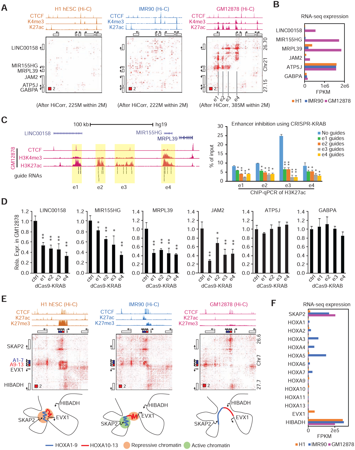
A-B, The bias corrected Hi-C heatmaps at a GM12878-specific enhancer aggregate (A), and the transcription levels of the six genes in this region (B). C, Left: Browser tracks showing the GM12878 ChIP-seq data and the locations of guide RNAs for the enhancer inhibition with sgRNAs-CARGO (STAR Methods). Right: ChIP-qPCR results showing the loss of H3K27ac occupancy after inhibiting each of enhancers. D, The expression levels of every gene when the four enhancers indicated in (A and C) are repressed using CRISPRi; data are representative from > 3 independent experiments. Error bar: s.d. of 3 PCR replicates; * p < 0.05, ** p < 0.01 in t test. E, Architecture of HoxA gene cluster in H1, IMR90 and GM12878 cells. F, Expression of HoxA genes in these three cell types.
With the removal of the local DNA packaging signal, we can also distinguish chromatin compaction events as red pixel domains. The best example is the Polycomb group (PcG) associated chromatin domain at HOXA gene family(Narendra et al., 2015; Noordermeer et al., 2011; Schoenfelder et al., 2015b). The normalization dimmed the up- and downstream TAD signal and allowed direct observation of the ESC-specific repressive chromatin domain at HOXA genes, which splits or dissolves when it loses some or all the H3K27me3 mark in IMR90 and GM12878 cells (Figure 3E–F).
Chromatin loops, but not compartments, mark neural cell fate and functions
We are particularly interested in identifying enhancer aggregates associated with neural differentiation, since they may represent a 3D genome signature for the neuronal lineage. To do this, we first identified 323,700 loop pixels in total from hiPSC, hNPC and hNeuron cells, each with ~140K pixels (Figure 4A). The overlap between hNeurons and hNPCs is greater than their overlap with hiPSCs (Figure 4A). The loop sizes in the three cell types are comparable (Figure 4B). Insulators (with CTCF), promoters (with H3K4me3), and enhancers (with H3K27ac) are clearly top contributors to chromatin loops (Figure 4C). Interestingly, the numbers of enhancer- or promoter interactions increased in hNPCs and hNeurons than in hiPSCs (Figure 4C). The genes involved in hNPC and hNeuron chromatin loops are strongly associated with neuronal differentiation functions (Figure 4D). We also collected GWAS SNPs reported for a number of neuronal or psychiatric phenotypes (including intelligence, autism, schizophrenia, Alzheimer’s disease, etc.) and found that they are enriched in the hNPC or hNeuron, but not the hiPSC chromatin loop regions; such enrichment is not observable for diabetes/obesity GWAS SNPs (Figure 4E).
Figure 4. Chromatin loops are hallmarks of neural differentiation and neural functions.
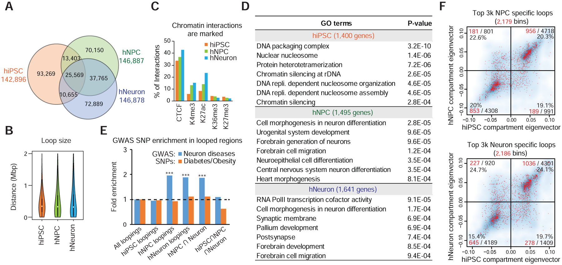
A, Venn diagram showing the overlap between chromatin interactions from hiPSCs, hNPCs and hNeurons. B, Distance distribution of chromatin loops in three cell types. C, Bar graph showing the percentage of chromatin interactions with various histone marks. D, Gene ontology terms for genes involved in top 3,000 chromatin loop pixels in each cell type ranked by ratio. E. Enrichment of neuron- or diabetes/obesity relevant GWAS SNPs at chromatin loops. ***p<0.001, binomial test. F, Compartment switching status of the hNPC- (upper) or hNeuron-specific (lower) loops. The four quadrants indicate the compartment-switching status after differentiation. Red dots: bins containing neural loops. All bins in the genome were plotted in the background as blue cloud. Number of red bins, total bins, and percentages are shown in each quadrant.
Because genome compartmentalization is also a good indicator for cell identity, we performed a compartment-level analysis of neuron differentiation at 250kb resolution. We identified 877 bins that switched their compartment in either hNPCs or hNeurons (Figure S5A–B and Table S3). Presumably, these dynamically compartmentalized regions (DCR) are relevant to neurogenesis. However, although we observed a consistent correlation between H3K27ac occupancy, PC1 values and overall gene expression (Figure S5C–E), gene ontology analysis failed to identify neuron related terms in these DCRs (Figure S5F). One plausible explanation is that low-resolution analysis lacks the precision to pinpoint neural genes. We therefore further tested the relationship between dynamic chromatin loops and compartment switching. The anchors of the strongest 3,000 hNPC-specific or hNeuron-specific (compared to hiPSC) chromatin loops involve more than 2,000 genomic bins in the compartment analysis (~20% genome, Figure 4F). Interestingly, a majority of neural loops, hence their anchored genes, are present in the unchanged compartments; there were no obvious enrichment of neural loops within the compartment-switching regions (Figure 4F). Furthermore, the genes anchored at neural loops are still enriched with neural terms in gene ontology analysis even after removing those within the compartment switch regions, (Figure S5G–H). These results indicate that neuronal gene activation frequently occur without the switching of compartments A and B; dynamic chromatin loops better marks neuronal differentiation than compartment switching.
E-P loops and aggregates mark neural differentiation but not gene activation
We next constructed a network of 6,067 promoters and 11,453 enhancers using the aforementioned chromatin loops. The network includes 1,939 connected components (i.e. connected subnetworks); nearly one-third (603) of them are candidate E-P aggregates (multi-node clusters with at least five edges, Figure S6A). We used the ratio of each loop pixel to measure the loop strength semi-quantitatively, and identified 174 neural E-P aggregates in which the chromatin loops are strengthened in hNeurons compared to hiPSCs (STAR Methods and Table S4). As expected, the neural enhancer aggregates contain key neural genes, including FOXG1, POU3F3, SOX11, and TCF4 (Figure 5A). Independent Hi-C data from hESCs and primary brain tissues also supported our observation that the E-P loops at these loci were gained during neural differentiation (Figure 5B, more examples in Data S1I). Interestingly, many of these enhancer aggregates are substantially strengthened in the primary brain tissues, sometimes form striking grid-like patterns (Figure 5B), suggesting that hNPCs and hNeurons are in a transition phase of genome rewiring; enhancers and promoters continue to aggregate and stabilize during neuronal maturation.
Figure 5. Identifying E-P aggregates associated with neurogenesis.
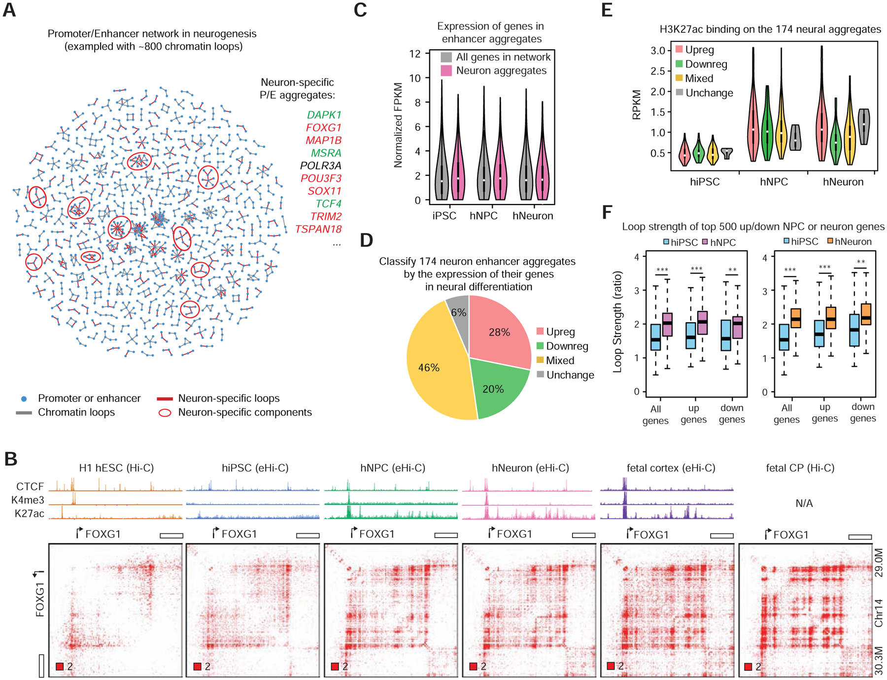
A, An exemplary enhancer-promoter network with ~800 chromatin loops during neurogenesis. Neuron-specific network components can be identified as candidate neuronal enhancer aggregates. Genes in a few neural enhancer aggregates are listed on the right: red, upregulated in neural differentiation, green, downregulated. B, Formation of enhancer aggregate at the FOXG1 locus during neural differentiation. C, Summary of gene expression in neural enhancer aggregates. D, Classification of neural enhancer aggregates based on their dynamic gene expression during differentiation. E, H3K27ac occupancy at different categories of neural enhancer aggregates. F, Compare the strength (ratio) of loop pixels at the differentially expressed genes (DEGs). Top 500 DEGs were picked by comparing hNPC (left) or hNeuron (right) to hiPSC. ***, p < 0.001; **, p< 0.01 Wilcoxon rank-sum test.
It is however surprising that the neural E-P aggregates do not correlate with gene activation (Figure 5C). Our RNA-seq data revealed that the 174 neural E-P aggregates contain both up- and down-regulated genes during neurogenesis (Data S1 I and Table S4), although they clearly gain higher overall H3K27ac occupancy in hNPC or hNeuron than in hiPSCs (Figure 5D–E). In fact, when we examined the loop pixels associated with dynamic genes in hNPC and hNeurons, both up-regulated and down-regulated genes showed stronger loop intensity compared to hiPSC (Figure 5F), consistent with the global trend that cells gain chromatin interactions at promoters and enhancers during differentiation (Figure 4C). We could not observe consistent loop strength difference between up- and down-regulated genes (Figure 5F). Furthermore, we also observed continuous E-P aggregation at several gene-dense regions in which genes are already active in hESCs and hiPSCs (marked by H3K4me3 and H3K27ac); these genes can be either up- or down-regulated in hNPCs and hNeurons in a coordinated fashion (Data S1 II and Table S4). All these results indicated that E-P aggregation during neurogenesis does not necessarily result in gene activation (see more discussion below).
The improved E-P interaction maps outperform eQTL in identifying GWAS target genes
Finally, we explored our dataset to investigate the genetics of brain disorders. We collected 6,556 lead GWAS SNPs reported for a number of cognitive traits or brain-related disorders (including intelligence, autism, schizophrenia, Alzheimer’s disease, etc.) (MacArthur et al., 2017) and defined their linkage disequilibrium (LD) using the latest TOPMed data (STAR Method). We next called 14,943 distal GWAS SNP-promoter pairs (i.e. the predicted promoter is outside of the GWAS LD) using chromatin loop data (Table S5). We defined tier 1 neural loop predictions as the SNP-promoter pairs supported by loops from >=2 of the six neural (e)Hi-C datasets. There are 4,421 tier1 pairs involving 2,173 SNPs and 1,439 genes (Figure 6A). Similarly, we also defined tier 2 and tier 3 loop predictions, which are supported by only one or zero neural (e)Hi-C datasets. Additionally, we also predicted distal GWAS target genes (outside of LD) using the GTEx cis-eQTL data from 48 human tissues(Consortium et al., 2017), including 14 neural tissues (13 brain tissues and nerve tibial) (Table S5). The overlap between loop and eQTL predictions is modest: 10.4%, 7.8%, and 7.5% of tier 1–3 neural loop predictions are supported by neural eQTLs. However, non-neural eQTL data also have a similar trend (18.4%, 14.7% and 15.4% for tier 1–3 loop predictions, Figure 6A), suggesting a lack of tissue specificity.
Figure 6. Chromatin loop outperforms eQTLs in explaining GWAS results.
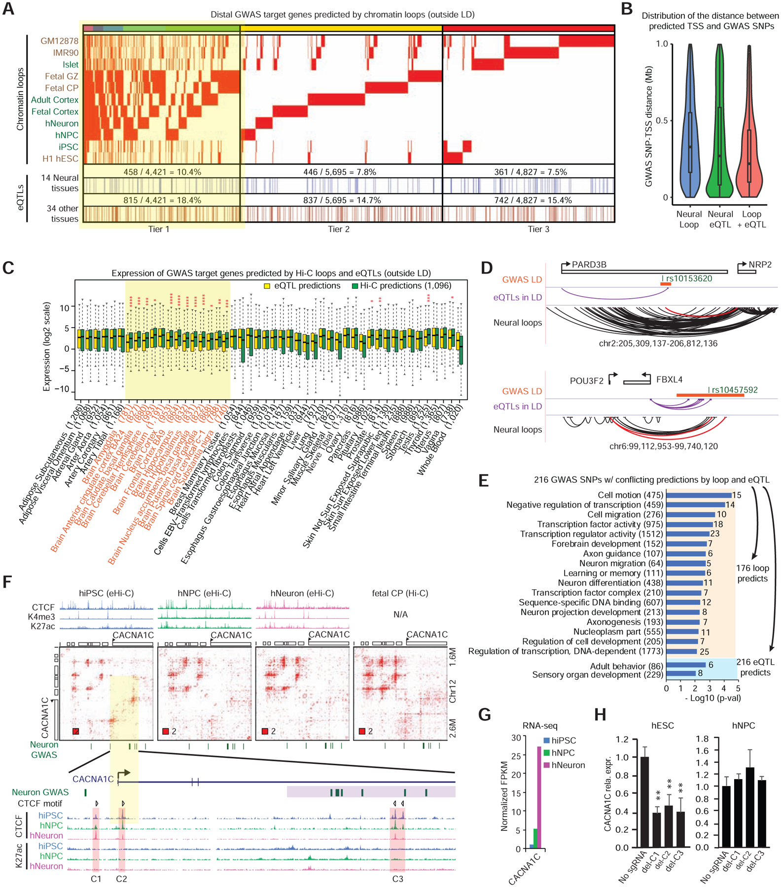
A, Heatmap showing the chromatin loop predicted GWAS target genes, and their overlap with GTEx eQTL data. Highlighted: Tier 1 neural predictions supported by at least two neural Hi-C datasets. B, Distance distribution of predicted GWAS SNP-TSS pairs, based on whether they are supported by loop, eQTL, or both. C, We used neural loops to predict 1,096 target genes for brain GWAS SNPs, and compared their expression to eQTL predicted genes in 48 GTeX tissues. Tissue with red stars: neural loop-predicted genes have higher expression levels than eQTL-predicted genes. *p<1e-2,**p<1e-3,***p<1e-4,****p<1e-5 Wilcoxon rank sum test; Highlighted in yellow: 13 brain tissues. Numbers in parenthesis: the number of genes predicted with eQTL data in each tissue. D, Two GWAS loci examples for which neural loop and eQTL make conflicting predictions. E, GO terms enriched in loop or eQTL predicted target genes, when the two methods make conflicting predictions. F, The CACNA1C GWAS locus is associated with an hiPSC-specific CTCF loop. Highlighted are the three CTCF occupied regions and the CTCF motif directionality. G, Expression of CACNA1C during neurogenesis using RNA-seq data. H, CTCF deletion downregulates CACNA1C in hESC but not NPC. Data are representative from > 3 independent experiments. Error bar: s.d. of three independent experiments; * p < 0.05, ** p < 0.01 in t test.
We therefore systematically compared the performance of chromatin loop and eQTL data in explaining GWAS results. We focused on tier 1 loop predictions only within 1Mb, since GTEx only called cis-eQTLs in this window (Figure 6B). Firstly, we setup a test comparing Hi-C and eQTL as two independent approaches predicting the target genes of distal GWAS SNPs. The test assumes that if we make predictions for brain GWAS SNPs, most target genes should be expressed in brain. (Similarly, if we made prediction for liver GWAS SNPs, most target genes should be expressed in liver.) According to this logic, when we analyze brain GWAS SNPs, if method A finds more brain-expressing genes than method B, we can say method A is better than B; as a result, genes predicted by method A should have higher average expression in brain than genes predicted by method B.
We predicted 1,096 target genes using neural chromatin loops (loop target genes). Using eQTL data from each of the 48 GTeX tissues, we also predicted 48 different sets of genes (eQTL target genes) for the same collection of GWAS SNPs (Figure 6C). In 12 of the 13 brain tissues, but less frequently in non-brain tissue (4 of 35), the expression levels of the 1,096 loop target genes are significantly higher than eQTL target genes (Figure 6C); such brain-specific difference (between loop- and eQTL-predictions) cannot be observed with randomly chosen GWAS SNPs (Data S1 III). These results indicate that the chromatin loops perform better than eQTLs in predicting brain GWAS targets.
We further focused on the 216 GWAS SNPs for which chromatin loops and brain eQTLs made conflicting prediction of target genes (Table S5). Figure 6D shows two such examples: one locus (rs10153620) associated with attention deficit hyperactivity disorder (ADHD) (Ebejer et al., 2013), and the other locus (rs10457592) associated with major depression (Hyde et al., 2016). In both examples, chromatin loop predicted key neuronal genes (NRP2 and POU3F2), while brain eQTLs predicted genes with unclear brain functions (PARD3B and FBXL4). Most importantly, we found an overall trend that chromatin loops outperform eQTLs in identifying genes with known brain functions. For all of the 216 GWAS SNPs, Hi-C predicted 176 target genes, which enriched dozens of GO terms related to neural functions and transcription regulation (Figure 6E and Table S5). In contrast, the eQTL target genes only enriched two relevant GO terms at a p < 0.01 level, highlighting the value of chromatin loop data in explaining disease genetics (Figure 6E, see discussion).
Interestingly, although we frequently observed neural loops at known brain GWAS loci, such as MEF2C, CTNND1, TRIO, and DRD2 (Data S1 IV), some loci lose chromatin loops during neural differentiation. The best example of this is the GWAS locus located in the third intron of CACNA1C, which is one of the strongest and best-replicated associations for schizophrenia (SCZ) and bipolar disorder (BD) (Moon et al., 2018). Past studies on this locus in neurons or brain tissues suggested a transcription regulatory role, but the causative variants are still unknown (Arnold et al., 2013; Eckart et al., 2016; Roussos et al., 2014; Song et al., 2018). Unexpectedly, we found a strong CTCF loop connecting the GWAS locus to the CACNA1C promoter only in hiPSC; the loop weakens when the gene is upregulated during neurogenesis and in brain tissues, possibly due to transcription elongation (Heinz et al., 2018) (Figure 6F–G). CACNA1C has a low (compared to hNPCs and hNeurons) but detectable expression in hESCs. To test if the CTCF loop is functional, we deleted the three corresponding CTCF binding sites and found that CACNA1C is downregulated only in hESCs but not in hNPCs (Figure 6H and Figure S6B–C). Therefore, our results indicated that the distal GWAS locus can be recruited to the CACNA1C promoter and regulate the gene expression.
It should be noted that our data did not suggest which variants in this locus regulate CACNA1C transcription; we found no common SNPs affecting CTCF sites in this GWAS locus. Our working model is that when the CTCF loop brings the GWAS locus to CACNA1C promoter, this locus gains a gene regulatory potential. As a result, genetic variants in the risk locus may affect CACNA1C expression. Since we only observed strong looping in hESCs, and this CTCF loop progressively weakened during neurogenesis, we speculate that the GWAS locus may affect gene expression and disease during early development instead of in mature neurons, which is consistent with a recent mouse study showing that CACNA1C affects psychological disorders during embryonic development instead of adult neurons (Dedic et al., 2018). It is necessary to point out that the expression level of CACNA1C is low in hESCs. More studies are necessary to determine: (i) the function of CACNA1C in ESCs or early development; (ii) the possibility that the loop might be present in certain brain cell types. Nevertheless, this example highlighted the importance of examining looping dynamics and cautions against only using brain or neuron data to investigate disease genetics.
Discussion
In this study we developed a low input “easy Hi-C” protocol for 3D genome mapping from 50–100K cells. We also developed a new analysis pipeline named HiCorr to improve the rigor of Hi-C or eHi-C bias-correction at high-resolution. We showed that HiCorr-correction significantly improved the sharpness of Hi-C heatmaps, and allowed direct recognition of E-P loops at sub-TAD level, with little interference from the local DNA packaging events. These results highlighted the importance of rigorous bias-correction in high-resolution Hi-C data analysis; we demonstrated that with HiCorr, robust Hi-C map of E-P interactions is achievable with a moderate read depth (~200 million mid-range cis-contacts). In many examples, the promiscuous TAD blocks in raw heatmaps become discrete E-P loops or aggregates after correction, indicating that promoters and enhancers form stable CTCF-independent interactions and are dominant contributors to intra-TAD signal.
Our Hi-C analysis revealed striking enhancer aggregation events during neurogenesis and in mature brain tissues. Many of these enhancer aggregates are near key neural genes. However, it is unexpected that differentiation-gained enhancer aggregates do not correlate with gene activation, since the enhancer “phase separation” model was initially proposed as a mechanism for trans-activation(Hnisz et al., 2017). It appeared that both up- and down-regulated genes gained enhancer interactions during neurogenesis (Figure 5C–F). Since recent studies have revealed multiple phase separation mechanisms that organize both euchromatin and heterochromatin (Erdel and Rippe, 2018), we speculate that even at enhancers, different trans- factors (protein or RNA) may create chromatin contacts during cellular differentiation, which do not necessarily cause gene activation. More studies are required on a case-by-case basis to tease out the underlying mechanisms, and to investigate whether the newly gained DNA contacts have gene regulatory functions.
Chromatin loops and eQTLs are two independent methods to identify long-range cis-regulatory relationships. When studying the function of non-coding variants, it is becoming common practice to look for evidence from both chromatin loop and eQTL data. However, our study showed a limited consistency between the two methods in predicting GWAS target genes: only a small fraction of looped GWAS loci are also supported by eQTLs. One possible explanation for this discrepancy is the lack of statistical power in eQTL detection, i.e. many cis-regulatory variants may not pass statistical significance due to: (i) limited population size; (ii) low minor allele frequency (MAF). However, the sensitivity issue cannot explain why loop appears to be more accurate than eQTL when the two methods make conflicting predictions (Figure 6D–E). Furthermore, a recent large blood eQTL study reported that after increasing the sample size to > 30,000 donors, although many more cis-eQTLs could be identified, they were mostly short-range eQTLs near promoters and had a different genetic architecture from GWAS SNPs(Võsa et al., 2018). The limited success of eQTLs in GWAS study highlighted another potential possibility that eQTLs obtained from healthy tissues may not reflect the gene regulatory landscape from patients. For example, a SNP may only have subtle effects on looped target gene in healthy donors, but plays a more prominent role when the locus gains a disease-specific enhancer in patients; in this scenario, chromatin loop can identify the correct target genes but eQTL from normal tissues cannot. Therefore, our results indicated that high-quality Hi-C loops have a unique value in the study of disease genetics: we should treat loops and eQTLs as two distinct lines of biological evidence in explaining GWAS results, rather than two mutually confirmatory datasets.
STAR METHODS
RESOURCE AVAILABILITY
Lead contact
Further information and requests for resources and reagents should be directed to and will be fulfilled by the lead contact, Fulai Jin (fxj45@case.edu).
Materials availability
All unique/stable reagents generated in this study are available from the Lead Contact with a completed Materials Transfer Agreement.
Data and code availability
Data for eHi-C protocol optimization (in IMR90 cells) are available at NCBI GEO with accession number GSE89324. Raw and/or processed eHi-C and ChIPmentation data in hiPSC, hNPC and hNeuron are available at NCBI GEO with accession number GSE115407. Newly generated Hi-C data in hESCs are also included in GSE115407. ChIP-seq and eHi-C from fetal or adult brain cortex are available at NCBI GEO with accession number GSE116825. This study also re-analyzed published Hi-C data and ChIP-seq data. The accession numbers of raw data are listed in Table S2 and Key Resources Table.
KEY RESOURCES TABLE
| REAGENT or RESOURCE | SOURCE | IDENTIFIER |
|---|---|---|
| Antibodies | ||
| Rabbit polyclonal anti-H3K4me3 | Abcam | Cat#ab8580; RRID:AB_306649 |
| Rabbit polyclonal anti-H3K27ac | Abcam | Cat#ab4729; RRID:AB_2118291 |
| Rabbit polyclonal anti-H3K27me3 | Millipore | Cat#07–449; RRID:AB_310624 |
| Rabbit polyclonal anti-H3K36me3 | Abcam | Cat#ab9050; RRID:AB_306966 |
| Rabbit polyclonal anti-CTCF | Abcam | Cat#ab70303; RRID:AB_1209546 |
| Biological Samples | ||
| Adult anterior temporal cortex | Dr Craig Stockmeier, University of Mississippi Medical Center | This study |
| Fetal cerebra | NIH NeuroBiobank | This study |
| Chemicals, Peptides, and Recombinant Proteins | ||
| Collagenase | Gibco | Cat#17104–019 |
| Dorsomorphin | Tocris | Cat#3093 |
| A83–01 | Tocris | Cat#2939 |
| Cyclopamine | Cellagen Technology | Cat#C2925–10 |
| BDNF | Peprotech | Cat#450–02 |
| GDNF | Peprotech | Cat#450–02 |
| Deposited Data | ||
| Data of eHi-C protocol optimization on IMR90 | This study | GEO: GSE89324 |
| Raw and analyzed data of H1 and neuron differentiation | This study | GEO: GSE115407 |
| Raw and analyzed data of brain tissues | This study | GEO: GSE116825 |
| Fetal CP and GZ HiC | Chromosome conformation elucidates regulatory relationships in developing human brain | GSM2054564, GSM2054565, GSM2054566, GSM2054567, GSM2054568, GSM2054569 |
| GM12878 HiC | A 3D Map of the Human Genome at Kilobase Resolution Reveals Principles of Chromatin Looping | GSM1551583, GSM1551584, GSM1551586 |
| GM12878 HiC | Whole-genome haplotype reconstruction using proximity-ligation and shotgun sequencing | GSM1181867, GSM1181868 |
| IMR90 Hi-C | A high-resolution map of the three-dimensional chromatin interactome in human cells | GSM1055800, GSM1055801, GSM1154021, GSM1154022, GSM1154023, GSM1154024, GSM1055802, GSM1055803, GSM1154025, GSM1154026, GSM1154027, GSM1154028 |
| H1 Hi-C | Chromatin architecture reorganization during stem cell differentiation | GSM1267196. GSM1267197 |
| H1 ChIP-seq: input, H3K4me1, H3K4me3, H3K27ac, H3K27me3, H3K36me3 | Roadmap Epigenomics Project | GSE16256 |
| H1 ChIP-seq: CTCF | ENCODE Project Consortium | GSM733672 |
| IMR90 input | A high-resolution map of the three-dimensional chromatin interactome in human cells | GSM1055808 |
| IMR90 CTCF | A high-resolution map of the three-dimensional chromatin interactome in human cells | GSM1055825 |
| IMR90 H3K4me1 | A high-resolution map of the three-dimensional chromatin interactome in human cells | GSM1055814 |
| IMR90 H3K4me3 | A high-resolution map of the three-dimensional chromatin interactome in human cells | GSM1055816 |
| IMR90 H3K27ac | A high-resolution map of the three-dimensional chromatin interactome in human cells | GSM1055818 |
| IMR90 H3K27me3 | Roadmap Epigenomics Project | GSE16256 |
| IMR90 H3K36me3 | A high-resolution map of the three-dimensional chromatin interactome in human cells | GSM1055820 |
| GM12878 input | ENCODE Project Consortium | GSM733742 |
| GM12878 CTCF | ENCODE Project Consortium | GSM733752 |
| GM12878 H3K4me1 | ENCODE Project Consortium | GSM733772 |
| GM12878 H3K4me3 | ENCODE Project Consortium | GSM733708 |
| GM12878 H3K27ac | ENCODE Project Consortium | GSM733771 |
| GM12878 H3K27me3 | ENCODE Project Consortium | GSM733758 |
| GM12878 H3K36me3 | ENCODE Project Consortium | GSM733679 |
| Source gel image | This study | DOI: 10.17632/tpvjrcg454.2 |
| Experimental Models: Cell Lines | ||
| IMR90 fibroblasts | ATCC | CCL-186 |
| H1 hESC | WiCell | WA01 |
| Human skin fibroblast CCD-1079Sk | ATCC | CRL-2097 |
| hNPC differentiated from hiPSC | This study | N/A |
| hNeuron differentiated from hiPSC | This study | N/A |
| DI-Cas9-H9 | This study | N/A |
| GM12878 | Coriell Institute | CEPH/UTAH Pedigree 1463 |
| Oligonucleotides | ||
| Oligos and primers used in this study (see Table S2) | This study | N/A |
| Recombinant DNA | ||
| Lenti-dCas9-KRAB-blast | Addgene | Cat#89564 |
| LentiCRISPRv2 | Addgene | Cat#98654 |
| px332-original plasmid | Joanna Wysocka (Gu et al., 2018) | N/A |
| CARGO plasmids | Joanna Wysocka (Gu et al., 2018) | N/A |
| Software and Algorithms | ||
| HiCorr | This study | https://github.com/JinLabBioinfo/HiCorr |
| Bowtie | Langmead et al., 2009 | http://bowtie-bio.sourceforge.net/index.shtml |
| Compartment level analysis | This study | https://github.com/shanshan950/compartment_analysis |
| Domain Caller | Dixon et al., 2013 | http://bioinformatics-renlab.ucsd.edu/collaborations/sid/domaincall_software.zip |
| ImageJ | Schneider et al., 2012 | https://imagej.nih.gov/ij/ |
| MACS | Zhang et al., 2008 | https://github.com/taoliu/MACS |
| NetworkX | Hagberg et al., 2008 | https://networkx.github.io/ |
| Cytoscape | Shannon et al., 2003 | https://cytoscape.org/ |
| Gene Ontology | DAVID Bioinformatics Resources | https://david.ncifcrf.gov/ |
The source code for HiCorr can be found in https://github.com/JinLabBioinfo/HiCorr.
The original gel images are available at Mendeley Data and can be found in http://dx.doi.org/10.17632/tpvjrcg454.2.
EXPERIMENTAL MODEL AND SUBJECT DETAILS
Cell lines
We used human primary IMR90 fibroblasts (ATCC, #CCL-186) to test eHi-C performance. IMR90 cells were grown as previously described(Jin et al., 2013). After confluence, the cells were detached with trypsin and collected by spinning down at 900g for 5 minutes. Then the cells were fixed in 1% formaldehyde for 15 minutes at 37°C, followed by 150mM glycine at room temperature for 5 minutes to quench formaldehyde. The fixed cells were washed in PBS and pelleted before stored in −80°C. We generated additional conventional Hi-C libraries for H1 hESCs (WiCell, #WA01) because published Hi-C data in H1 hESC are not deep enough to support the fragment resolution analysis. H1 cells were cultured on the hESC-qualified Matrigel (Corning, #354277) coated plates in mTeSR1 medium (StemCell Technologies, #05850) before harvested for Hi-C analysis. The cell fixation protocol is the same as IMR90 cells.
Neurogenesis samples
The hiPSC line used for neurogenesis has been previously extensively characterized, including expression of pluripotent markers, karyotyping, lack of transgene integration, demethylation of promoter regions of pluripotent genes, in vitro differentiation into cell types of three germ layers and teratoma formation(Chiang et al., 2011; Wen et al., 2014). We followed our previously established protocol for forebrain-specific neuronal differentiation (Wen et al., 2014). Briefly, hiPSC colonies were lifted by 1 mg/ml collagenase (Gibco, #17104–019) and cultured in non-treated polystyrene plates with embryoid body (EB) medium consisting of 20% KOSR (Knockout Serum Replacement, Gibco, #10828–028), 2 μM dorsomorphin (Tocris, #3093) and 2 μM A83–01 (Tocris, #2939) for 7 days with daily medium changes. The EBs were then attached on matrigel to develop organized rosette-like structure and maintained in neural induction medium (hNPC medium) with an equal mixture of DMEM/F12 (Gibco, #11330–032) and Neural basal medium (Gibco, #21103–049), N2 supplement (Gibco, #17502–048), B27 supplement (Gibco, #17504–044), NEAA (MEM Non-Essential Amino Acids Solution, Gibco, #11140–050) and 2 μM cyclopamine (Cellagen Technology, #C2925–10) for 16 days with medium change every other day. The neural rosettes were harvested mechanically and transferred to low attachment plates (Corning, #3473) in hNPC medium to form neural spheres for 3 days. hiNPCs were expanded as monolayer in hNPC medium after dissociation of neural spheres by Accutase (Gibco, #A1110501). For neuronal differentiation, monolayer hiNPCs were switched to Neurobasal medium with 10 ng/ml BDNF (Peprotech, #450–02), 10 ng/ml GDNF (Peprotech, #450–02), GlutaMaxTM (Gibco, #35050061) and B27 supplement. Immunostaining was done as previously described (Wen et al., 2014). Quantification of different cellular markers was performed by analyzing a minimum of 500 cells from at least 4 randomly chosen fields of fluorescent images with ImageJ software. The cell fixation protocol is the same as IMR90 cells.
Brain tissues
For brain tissue analysis, anterior temporal cortex was dissected from postmortem samples from three adults of European ancestry with no known psychiatric or neurological disorder (Dr Craig Stockmeier, University of Mississippi Medical Center). Cerebra from three fetal brains were obtained from the NIH NeuroBiobank (gestational age 17–19 weeks), and none were known to have anatomical or genomic disease (Table S2). Samples were dry homogenized to a fine powder using a liquid nitrogen-cooled mortar and pestle. All samples were free from large structural variants (>100 kb) detectable using Illumina OmniExpress arrays. Genotypic sex matched phenotypic sex for all samples. For easy Hi-C, Pulverized tissue (~100 mg) was crosslinked with formaldehyde (1% final concentration) and the reaction was quenched using glycine (150 mM). We lysed samples on ice with brain tissue-specific lysis buffer (10 mM HEPES; pH 7.5, 10 mM KCl, 0.1 mM EDTA, 1 mM dithiothreitol, 0.5% Nonidet-40 and protease inhibitor cocktail). Samples are Dounce homogenized before HindIII digestion.
Colon crypt tissues
Crypts were dissected from non-cancer colon mucosa. After removing from the patient, we first cut away non–colon mucosa as much as possible, such as muscles, blood vessels and fat. The tissue was then treated with Cell dissociation buffer (Gibco, #13151–014) to pop out crypts from surrounding mucosa tissue. The suspension was filtered through a 300uM cell strainer to remove remaining tissue pieces. Pelleted crypts were crosslinked in 1% formaldehyde followed by glycine quenching. The fixed crypts were used for eHi-C as described below.
METHODS DETAILS
Easy Hi-C
The overview of eHi-C design
In Hi-C, 5’ overhangs are created after restrictive DNA digestion (e.g. with HindIII) so that ligation junctions can be labeled with biotinylated nucleotides and eventually enriched in a pull-down step with streptavidin beads. However, this biotin-dependent strategy has several intrinsic limitations that prevents the application of Hi-C in rare tissue or small cell populations. First, the efficiency of biotin incorporation into DNA is usually ~20–30%, sometimes as low as 5%(Belton et al., 2012). Therefore, a majority of ligation junctions cannot be recovered. Second, only a portion of labeled ligation junction products can be pulled-down after several washes, further lowering the recovery rate. Lastly, extensive washes are required in the biotin-pulldown procedure to effectively remove contamination of un-ligated DNA products, but this will significantly reduce the library complexity.
We reasoned that we might circumvent the limitations of Hi-C by using a biotin-free strategy to enrich ligation products, thus improving the assay efficiency. Inspired by the biotin-free strategies used in 4C(Simonis et al., 2006) and ELP(Tanizawa et al., 2010), we developed eHi-C, which only involves a series of enzymatic reactions to generate DNA libraries for the mapping of genome architecture (Figure 1A). In this protocol, we begin with the in situ proximity ligation procedure in which we performed HindIII digestion and proximity ligation while keeping nuclei intact(Nagano et al., 2013; Nagano et al., 2015; Rao et al., 2014). In eHi-C, HindIII digested chromatins were ligated without end repair, leading to HindIII-digestible junction products (Figure 1A). After nuclear lysis and reverse crosslinking, the DNA are digested with more frequent 4-base cutter DpnII before self-ligation. DNA with DpnII restrictive overhangs on both ends, including ligation junction products, will form circles. We used exonuclease to remove DNA that failed to form circles, as well as contaminations from un-ligated ends and other linear DNA species. At last, we cut the circularized DNA again with HindIII; only re-linearized junction DNA will be sequenced (Figure 1A).
The eHi-C method is essentially a genome-wide “all-to-all” version of 4C and also closely similar to ELP, another biotin-free genome-wide method developed several years ago to identify DNA contacts in fission yeast(Tanizawa et al., 2010). However, the design of ELP was flawed because it cannot remove contaminations from several species of non-junction DNA (Figure S1A). As a result, less than 4% of ELP reads represent proximity ligation events(Tanizawa et al., 2010). The eHi-C protocol solves this issue by introducing an exonuclease digestion step. Additionally, because all reads from ELP are next to HindIII sites, it cannot distinguish PCR duplicates from reproducible ligation events between the same pair of HindIII ends (Figure S1B). Our eHi-C method addresses this issue with a custom adapter with random barcode as a unique molecule index (UMI) (Figure 1A, Figure S1C). We also used in situ ligation in eHi-C to improve the library quality (Figure 1A). Taken together, we have significantly optimized the eHi-C strategy to obtain high quality libraries for ultra-deep sequencing from small-scale bio-samples, which is not feasible with the original ELP method.
Because there is theoretically no DNA loss in its protocol (Figure 1A), eHi-C should have a higher recovery rate of ligation junction products than conventional Hi-C, which is important for the analyses of small cell populations. The only exception is the exonuclease digestion step: Ligation junction DNA may be digested if they fail to self-ligate (Figure 1A). From a control experiment, we determined that the efficiency of the self-ligation reaction is high (~60%, Figure S1D).
Easy Hi-C protocol
In this study, low-input eHi-C libraries were prepared in two settings. In the first scenario (“aliquot” setting), we started with 1 million IMR90 cells and go through the protocol described below and usually resulted in ~250–500ng DNA for library preparation (Figure 1A). 10% or 20% of these DNA were used to generate library (0.1 or 0.2 million cells per library). In the second scenario (“mini” setting), we started the experiments with lysing 0.1 or 0.2 million cells following the same protocol as described below, except that all steps before library preparation were performed in 25% volume. Because the cell lysis and HindIII digestion conditions are different from the published in situ Hi-C protocol. We have made modifications in order to ensure nuclei integrity during ligation.
Cell lysis, HindIII digestion, and in situ ligation.
Cell pellet from ~1 million cells was lysed in 1ml cell lysis buffer (10mM Tris-Cl, pH7.5, 10mM NaCl, 0.2% NP-40, 1X proteinase inhibitor cocktail (Roche, #118735800001)) before incubating on ice for 15 minutes. If there is cell clump in the tube, we dounce the cells for 10 times every cycle for 3 cycles, with one-minute on ice between each cycle. After douncing, the nuclei were put on ice for another 5 minutes and then pelleted by centrifuging (2,500g for 5 minutes at 4°C). The pellets were washed once in 1X Cutsmart buffer (NEB) before resuspended in 360ul 1X Cutsmart buffer. After resuspension, 40ul of 1% SDS were added (final 0.1%), and the tubes were incubated at 65°C for 10 minutes. To quench the SDS, 44ul of 10% Triton X-100 (final 1%) was then added to each tube. For chromatin digestion, 400U HindIII (NEB, #R3104M 100U/μl) were added to each tube followed by incubation at 37°C for 4 hours. To ensure efficient digestion, another 400U of HindIII were added to each tube again for overnight digestion. On day 2, we digested the nuclei for another 4 hours by adding fresh HindIII enzyme (400U). After digestion, the enzyme was inactivated by adding 40ul of 10% SDS (final 1%) to each tube and incubation at 65°C for 20 minutes. The digested products were then transferred to a new 15ml tube and mixed with 3.06ml 1.15X ligation buffer (75.9mM Tris-HCl, ph7.5, 5.75mM DTT, 5.75mM MgCl2 and 1.15mM ATP). 187ul 20% Triton X-100 was added to the mixture and incubated at 37°C for 1 hour. For ligation, the products were then mixed with 30ul of T4 DNA ligase (Invitrogen, #15224–025, 1U/ul) and incubated at 16°C overnight. After ligation, the tubes were put at room temperature for 30 minutes and the nuclei were pelleted by centrifuging at 2,500g for 5 minutes. The supernatant was discarded to remove the free DNA and only the nuclei pellets were kept. The nuclei pellet step is skipped in the “dilute” libraries in Table S1. The nuclei pellets were then resuspended in 3.06ml of 1.15X ligation buffer and mixed with 40ul of 10% SDS and 187ul of 20% Triton X-100 for nuclear lysis.
Reverse crosslinking, DpnII digestion and self-ligation.
After nuclear lysis, the mixture was then reverse crosslinked at 65°C overnight after adding 25ul of 20mg/ml proteinase K. DNA were purified with Phenol: Chloroform: Isoamyl Alcohol (25:24:1) (Affymetrix, #UN2922) following standard protocol. ~2–3μg DNA are expected from 1M cells. The DNA was then digested with 50U DpnII (NEB, #R0543L, 10U/μL) in a total volume of 100uL at 37°C for 2 hours. After digestion, the enzyme was heat inactivated at 65°C for 25 minutes. The mixture was first incubated with 0.5 volume of PCRClean DX beads (Aline Biosciences) at room temperature for 10 minutes before harvesting the supernatant according to vendor’s protocol. The supernatant was then incubated with 2 volumes of PCRClean DX beads at room temperature for 10 minutes. DNA on the beads was then harvested in 300ul nuclease free water. The two-step bead purification results in DNA with a size range ~100–1,000bp. The DNA products were then mixed with 200ul of 5X ligation buffer, 5U T4 DNA ligase (Invitrogen, #15224–025, 1U/ul) and water to a total volume of 1ml. Self-ligation was done by incubating the tubes at 16°C overnight.
Exonuclease digestion and DNA circle re-linearization.
The self-ligated DNA were purified again with Phenol: Chloroform: Isoamyl alcohol and digested with 6U of lambda exonuclease (NEB, #M0262S) in 200μL volume at 37°C for 30 minutes. The exonuclease was then inactivated by incubating at 65°C for 20 minutes. Resulting DNA were purified with 2 volumes of PCRClean DX beads as described above. For DNA circle re-linearization, bead bound DNA were eluted and digested with 20U HindIII again at 37°C for 2 hours in 150μL volume. The HindIII enzyme was inactivated at 65°C for 20 minutes, and the DNA was purified with 2 volume PCRClean DX beads for another time as described above. In the end, bead-bound DNA was eluted in 50ul nuclease free water. From 1M cells, we expect 250–500ng DNA in the end.
Library preparation.
We took ~10–20% of re-linearized DNA (~50ng) for library generation following Illumina TruSeq protocol. Briefly, the DNA was first end repaired using End-it kit (Epicentre, #ER0720). The end-repaired DNA was then A tailed with Klenow fragment (3′–5′ exo–; NEB, #M0212L) and purified with PCRClean DX beads. Bead bound DNA were eluted in 20μL water and then reduced to 4μL using Speedvac at 50°C. The 4ul DNA product was mixed with 5ul of 2X quick ligase buffer, 1ul of 1:10 diluted annealed adapter (10uM) and 0.5ul of Quick DNA T4 ligase (NEB, #M2200L). The ligation was done by incubating at room temperature for 15 minutes and the enzyme was then inactivated by incubating at 65°C for 10 minutes. DNA was then purified with 1.8 volume of DX beads as described above. Elution was done in 14ul nuclease free water. For checking eHi-C library quality, we only needed to sequence less than 1 million reads on MiSeq (Illumina). Because the proportion of PCR duplicates from low-depth sequencing is very low, we used regular TruSeq indexed adapters (Illumina) without UMI barcode. To deep sequence an eHi-C library, we used custom TruSeq adapter in which the index is replaced by a 6 base random sequence. The custom adapter was generated by annealing the following two oligos: Universal oligo – AATGATACGGCGACCACCGAGATCTACACTCTTTCCCTACACGACGCTCTTCCGATC*T UMI oligo -- /5Phos/GATCGGAAGAGCACACGTCTGAACTCCAGTCACNNNNNNATCTCGTATGCCGTCTTCTGCTT*G
PCR amplification of DNA libraries.
To amplify the DNA libraries, we mixed 13ul adapter ligated DNA with 1ul of 20uM oligo C (AATGATACGGCGACCACCGAGATCTACAC), 1ul of 20uM oligo D (CAAGCAGAAGACGGCATACGAGAT) and 15ul of 2X KAPA HiFi Hotstart ready mix (Kapa Biosystems, #KK2602). And the PCR amplification was done as follows: denature at 98°C for 45 seconds, cycle at 98°C for 15 seconds, 60°C for 30 seconds, 72°C for 30 seconds, and we did 5 cycles at first for estimating the total cycle number needed, and then further extension at 72°C for 5 minutes. The products were then purified using 1.8 volume of PCRClean DX beads (Aline Biosciences, #C-1003–50) to remove primer contamination as described above. And the DNA was eluted in 20ul nuclease free water. And library quantification was done following the protocol of Illumina library quantification kit (KAPA Biosystems, #KK4824). PCR was done again in 50μL volume for a target final concentration ~20–40nM (usually ~3–4 additional cycles). The generated libraries were then subjected to sequencing.
ChIPmentation
We used ChIPmentation(Schmidl et al., 2015) to map histone modification and/or CTCF in different samples. Briefly, cells and tissues were fixed in 1% formaldehyde at room temperature for 15 minutes followed by glycine quenching. To isolate nuclei, we lysed brain tissues with a specific lysis buffer (10 mM HEPES; pH 7.5, 10 mM KCl, 0.1 mM EDTA, 1 mM dithiothreitol (DTT), 0.5% Nonidet-40 and protease inhibitor cocktail) for 10 minutes at 4°C. For cell cultures, we used lysis buffer 1 (50 mM HEPES; pH 7.5, 140 mM NaCl, 1 mM EDTA, 10% glycerol, 0.5% Nonidet-40, 0.25% Triton X-100 and protease inhibitor cocktail) for 10 minutes at 4°C. The collected nuclei were then washed with a lysis buffer II (200mM NaCl, 1mM EDTA pH8.0, 0.5mM EGTA pH8.0, 10mM Tris-Cl pH8.0 and protease inhibitor cocktail) for 20 minutes at room temperature. The nuclei were pelleted at 1,800g for 10 minutes at 4°C and then resuspended in lysis buffer III (10mM Tris-Cl pH8.0, 100mM NaCl, 1mM EDTA, 0.5mM EGTA, 0.1% Na-Deoxycholate, 0.5% N-lauroylsarcosine and protease inhibitor cocktail) for sonication. The chromatin was sheared for 10 cycles (15 seconds on and 45 seconds off at constant power 3) on Branson 450 sonifier. 20–50ug of chromatin was used for each H3K4me3 (Abcam, #ab8580)/ H3K27Ac (Abcam, #ab4729)/ H3K27me3 (Millipore, #07–449)/ H3K36me3 (Abcam, #ab9050) pulldown and 100–150ug for each CTCF (Abcam, #ab70303) pulldown. First, 11ul of Dynabeads M-280 (Life Technologies, Sheep Anti-Rabbit IgG, #11204D) was washed three times with 0.5mg/ml of BSA/PBS on ice and then incubated with designated antibody for at least 2 hours at 4°C. The beads/antibody complexes were then washed with BSA/PBS. The pulldown was done in binding buffer (1% Trixon-X 100, 0.1% Sodium Deoxycholate and protease inhibitor cocktail in 1X TE) by mixing the beads/antibody complexes and chromatin. After pulling down for overnight, the beads/antibody/chromatin complexes were washed with RIPA buffer (50mM HEPES pH8.0, 1% NP-40, 0.7% Sodium Deoxycholate, 0.5M LiCl, 1mM EDTA and protease inhibitor cocktail). The beads complexes were then subjected to ChIPmentation by incubating with homemade Tn5 transposase in tagmentation reaction buffer (10mM Tris-Cl pH8.0 and 5mM MgCl2) for 10 minutes at 37°C. To remove free DNA, beads were washed twice with 1x TE on ice. The pulldown DNA was recovered by reversing crosslink for overnight followed by PCRClean DX beads (Aline Biosciences, #C-1003–50) purification. To generate ChIP-seq libraries, PCR was applied to amplify the pulldown DNA with illumina nextera primers. Size selection was then done with PCRClean DX beads to choose the fragments ranging from 100bp to 1000bp.
CRISPR experiments
Generating doxycycline inducible Cas9 expressing hESC line (DI-Cas9-H9)
The DI-Cas9-H9 cells were generated as previously described (Ma S et al., 2018). Briefly, the pBlue-AAVS1-Puro-Cas9-M2rtTA-AAVS1 HITI donor plasmid was constructed by ligating the HindIII restricted Puro-Cas9-M2rtTA fragment cut out from the Puro-Cas9-M2rtTA plasmid to the pBlue-AAVS1-AAVS1 vector linearized with HindIII. To construct the Puro-Cas9-M2rtTA plasmid, CAG-M2rtTA-pA sequence was amplified from Neo-M2rtTA plasmid and subcloned into the Puro-Cas9 plasmid linearized with MfeI and MluI. To construct the pBlue-AAVS1-AAVS1 plasmid, a pair of oligos for AAVS1 gRNA targeting sequence (g-AAVS1-F: TCACCAATCCTGTCCCTAGGTTTA; g-AAVS1-R: CTAGGGACAGGATTGGTGACGGTG) were annealed and ligated to the pBlue vector linearized with XhoI and NotI. H9 cell line was maintained on Matrigel (Corning, #354277) in mTeSR1 (STEMCELL Technologies, #85850/05850). Cells were cultured at 37 °C in a humidified atmosphere with 5% CO2 in air. Cells were passaged with TrypLE (Gibco, #12604–021). Transfection was done using electrotransfection (1 pulse, 300 V, 4 ms, BTX). A total of 25μg plasmid (donor: Cas9: gAAVS1RNA = 3: 3: 2) was used in each electroporation. Around 4~9 million cells were resuspended with 500μL PBS in a 0.4 cm cuvette. Two days later, 0.5μg/mL puromycin was used to treat cells for 3 days. Cells were allowed to grow visible colonies for about 10 days, and then the colonies were picked into 96-well plate. Colonies were expanded and identified by PCR and sequencing (5-F: GGTTAATGTGGCTCTGGTT; 5-R: CTTGTACTCGGTCATCTCG; 3-F: TGACGGTTCACTAAACGAG; 3-R: AGAGGTTCTGGCAAGGAG).
Deleting CTCF sites in ESCs and NPCs with sgRNAs-CARGO
We made CARGO(Gu et al., 2018) constructs whenever we need to transfect multiple sgRNAs into the same cell. With CARGO system, we could assemble 4–10 sgRNAs simultaneously into one plasmid following the protocol described by Gu et al.(Gu et al., 2018). The CARGO plasmids are gifts from the laboratory of Joanna Wysocka. All sgRNAs were designed on CCTop-CRISPR/Cas9 target online predictor (https://crispr.cos.uni-heidelberg.de/) and manually picked. For CARGO, (n+1) pairs of oligos are necessary to assemble n sgRNAs. The CARGO oligo sequences are listed in Table S2. We deleted three CTCF-containing regions at CACNA1C locus (C1~C3). Successful deletion was verified with PCR. The primers used for detecting deletion efficiency are as follows: C1 (Product length wt: 616 bp, del: 471–518 bp; fwd: ACAGGATGCTATGGGACACC; rev: AGGGAGGAGGAAGAAATGGA); C2 (Product length wt: 786 bp, del: 531–603 bp; fwd: CCTGGGGTGTTGAGAGAGAA; rev: ATTCACCCAAAAGGCTTCCT); C3 (Product length wt: 9,358 bp, del: 550–600 bp; fwd: TGAGCCCAAAGGCACTAGAC; rev: TACCCAGAACAGGCACTTCC).
DI-Cas9-H9 cells were maintained in mTeSR1 medium (STEMCELL technologies, #85850) on matrigel. Cells were detached and suspended to single cells by Accutase (Fisher, #A1110501). CARGO vector transfection was done following the manufacturer’s instruction of Amaxa 2b nucleofector, using Kit 1 (Lonza, Human stem cell nucleofector Kit 1, #VPH-5012) and program B-16. After 24 hours recovery, cells were treated with 1μg/mL of Doxycycline to induce Cas9 expression for 48 hours before harvesting. The hNPCs were differentiated as described above and seeded at 170k cells per cm2. Transfection was done following the manufacturer’s instruction of Amaxa 4D nucleofector. Briefly, cells were treated with Accutase to make single cell suspension and then pelleted at 110g for 5min. P3 primary cell 4D-nucleofector X kit L (Lonza, #V4XP-3024) was applied combining program CU-133. After 24 hours recovery, cells were treated with 1μg/mL of Doxycycline to induce Cas9 expression for 48 hours before harvesting for DNA and RNA extraction.
Construct dCas9-KRAB-puro for CRISPRi assay
EF1-dcas9-KRAB was PCR amplified from Lenti-dCas9-KRAB-blast (Addgene, #89564) with primers (F: CCTTTTGCTCACATGTGCTAGCTGCAAAGATGGATAAAG, R: AACTTTGCGTTTCTTTTTCGGAACTGATGATTTGAT); T2A-puro was PCR amplified from the LentiCRISPRv2 plasmid (Addgene, #98654) using primers (F: AAGAAACGCAAAGTTGGATCCGGCGCAACAAACTTC, R: CGAGCTCTAGGAATTCTCAGGCACCGGGCTTGCG). The two PCR products were assembled into px332-original plasmid (gifts from the laboratory of Joanna Wysocka(Gu et al., 2018)) between PciI and EcoRI sites by In-Fusion HD cloning (TAKARA, #639648).
CRISPRi enhancer inhibition in GM12878 cells with sgRNAs-CARGO
We constructed CARGO vectors containing multiple sgRNAs as described above. GM12878 cells (Coriell Institute, #CEPH/UTAH Pedigree 1463) were maintained in RPMI1640 with 15% FBS. GM12878 cells were seeded in fresh medium at 350k cells per ml the day before nucleofection. 4 million cells were used for each nucleofection. First, cells were pelleted at 90g for 5min and then resuspended in 100ul of nucleofection reagent (SF cell line 4D-Nucleofector X kit, Lonza, #V4XC-2024) together with 5–7ug designated plasmids. The nucleofection was done on a 4D lonza nucleofector using program CM-137. Puromycin selection was done at 3μg/mL for 48 hours after letting the cell recover for 24 hours post transfection. Cells were then harvested for RNA extraction, or fixed with 1% formaldehyde. We performed H3K27ac ChIP-qPCR using ChIP-mentation protocol described before. 10% of chromatin was saved as input control. The qPCR and ChIP-qPCR primers used are listed in Table S2.
3C-qPCR
To confirm whether deletion of CTCF at the CACNA1C locus would lead to loss of chromatin loops, we did 3C assay in hESCs. We followed the protocol as previously described(Miele et al., 2006). First, H9 cells harboring CTCF deletion were generated as above by nucleofection and fixed for 3C assay. Briefly, Cells were permeabilized in a lysis buffer (10mM Tris-Cl, pH8.0, 10mM NaCl, 0.2% NP-40 and 1X proteinase inhibitor cocktail), and nuclei were collected by centrifuging at 2500g for 5min. The nuclei were then digested with HindIII-HF (NEB, #R3104M), 400U for 5 million cells at 37 °C overnight. After inactivation of HindIII, the proximity ligation was done with T4 DNA ligase (Invitrogen, #15224–025) at 16°C for overnight. Chromatins were then reverse-linked by proteinase K and purified by phenol: chloroform. Two BAC clones (RP11–265G12 and RP11–698B23) cover the studied region were applied as genomic background control. Equal moles of the DNA from two BACs were mixed together and used to generate the control template following the protocol. Primers designed for 3C-qPCR are listed Table S2.
QUANTIFICATION AND STATISTICAL ANALYSIS
The overview of eHi-C performance
We tested eHi-C in low-input setting with ~0.1–0.2 million human primary lung fibroblast IMR90 cells and used low- or high-depth sequencing to evaluate the library quality (Table S1). As expected, averagely 95% of eHi-C reads begin with digested HindIII restrictive sequence AGCTT, indicating that nearly all reads are from re-linearized HindIII-digestible DNA circles. When one eHi-C library from 0.1 million cells is deep-sequenced to 150 million mapped read pairs, the percentage of PCR duplicates is lower than the published IMR90 Hi-C libraries prepared with 100 times more (10 million) cells(Jin et al., 2013) (Table S1), indicating a significantly improved library complexity.
We also compared the sources of errors in Hi-C and eHi-C libraries(Belton et al., 2012; Jin et al., 2013). In conventional Hi-C, read pairs falling into the same HindIII fragments are considered invalid, and the major type of invalid reads are “dangling reads” originated from non-ligation DNA. In contrast, the only type of invalid pairs from eHi-C are self-circles, all the other types of invalid pairs are removed by exonuclease treatment (Figure S1E).
While eHi-C avoids several types of common false reads found in Hi-C, it has a drawback of getting false reads from undigested HindIII sites, which can be computationally filtered as back-to-back read pairs next to the same restrictive sites (Figure S1E–F). After data filtering, we found that the yield of cis-contacts from eHi-C libraries, especially the ones prepared with in situ ligation procedure, is better than most of the published HindIII-based Hi-C libraries prepared with ~10–25 million cells (Figure S1G–H and Table S1). Importantly, the contact heatmaps from Hi-C and eHi-C data are identical showing the same component A/B(Lieberman-Aiden et al., 2009) and TAD(Dixon et al., 2012) structures (Figure 1B–C). All these results demonstrated that eHi-C is a reliable alternative to Hi-C and can correctly identify 3D genome features from small cell populations.
Easy Hi-C data pre-processing for QC and performance analysis
Note: The data filtering step of deep Hi-C and eHi-C data for fragment level analysis is slightly different from the performance analysis here. Please refer to “Hi-C and eHi-C data filtering for fragment level analysis” for details.
Alignment and removing PCR duplications
Published IMR90 Hi-C data are used in this study to compare with eHi-C. The accession numbers of Hi-C data are listed in Table S2. All the sequencing data are mapped to human reference genome hg19 using Bowtie. For Hi-C, the two ends of paired-end (PE) reads were mapped independently using the first 36 bases of each read. PCR duplications were defined as PE reads with both ends mapped to the same locations. For eHi-C, because nearly all the mappable reads start with HindIII sequence AGCTT, we trimmed the first 5 bases from every read, took the next 36 bases, and added the 6-base sequence AAGCTT to the 5’ of every read before mapping using the whole 42 bases. Some MiSeq runs were performed with reads shorter than 41 bases, and the full-length reads will be used in those cases. After mapping, we further filtered the reads requiring the positions of both ends to be exactly at the HindIII cutting sites. The deep sequenced eHi-C libraries were prepared with UMI adapter, PCR duplications were defined as identical PE reads also with the same UMI barcode. The eHi-C libraries sequenced on MiSeq were not intended for deep sequencing and therefore were prepared without UMI barcode. We assume no PCR duplication in MiSeq libraries because the sequencing depth is very low.
Conventional Hi-C data filtering and QC analysis
After removing PCR duplications, we analyzed the library quality by classifying the reads into different categories. In both Hi-C and eHi-C, the percentage of trans- contacts can be easily calculated by counting the number of reads with two ends on different chromosomes (listed in Table S1). For cis- reads in Hi-C data, we first discard the reads with both ends mapped to the same HindIII fragments as invalid pairs. Dangling ends are defined as “inward” pairs among the invalid pairs (Figure S1E) and the percentages are listed in Table S1. The rest of the invalid pairs are classified into “other false” category.
All rest read pairs represent two different HindIII fragments in cis. Since cut-and-ligation events are expected to generate reads within 500bp upstream of HindIII cutting sites due to the size selection (“+” strand reads should be within 500bp upstream of a HindIII site, and “−” strand reads should be within 500bp downstream a HindIII site), we only keep read pairs with both ends satisfying this criteria. The other pairs are also classified into “other false” category in Table S1. We next split all the remaining reads into three classes based on their strand orientations (“same-strand”, “inward”, or “outward”) (Figure S1E). We have previously shown that although theoretically “same-strand” reads should be twice as many as “inward” or “outward” reads, in reality more “inward” or “outward” reads can be observed due to incomplete digestion of chromatin(Jin et al., 2013). We therefore estimate the total number of real cis-contact as twice the number of valid “same-strand” pairs (Table S1).
eHi-C data filtering and QC analysis
For eHi-C library, the only type of invalid cis- pairs are self-circles with two ends within the same HindIII fragment facing each other (Figure S1E). Similar to Hi-C, we also computed the total number of real cis-contact as twice the number of valid “same-strand” pairs. Reads from undigested HindIII sites are back-to-back read pairs next to the same HindIII sites facing away from each other (Figure S1F).
Compare the bias structure of Hi-C and eHi-C
Summary:
We analyzed the intrinsic biases that may affect the eHi-C experimental procedure. As expected, both Hi-C and eHi-C show a decay of contact frequency with increasing distance (Figure S1K). The contact frequencies involving very small HindIII restriction fragments (< 200bp) are low in both Hi-C and eHi-C libraries, because the small fragments are less likely to be sheared or digested (see STAR Methods), or due to the spatial hindrance for small fragments to ligate (Figure S1L)(Yaffe and Tanay, 2011). The eHi-C has an overall better performance capturing ligation between small-sized (~200bp-1kb) fragments (Figure S1L, M and P), presumably because DpnII can digest small HindIII fragments effectively as long as the restrictive sites are present. Furthermore, the profile of distance decay at short range is affected by the length of the two HindIII fragments (Figure S1M and 1P), indicating an interaction between the three parameters. Intriguingly, the GC-bias profile in eHi-C library is opposite to what was observed for conventional Hi-C(Yaffe and Tanay, 2011) (Figure S1N). We speculate that this might be because both ends of the eHi-C library start with a fixed HindIII restrictive sequence (AGCTT). Therefore, the GC-bias in eHi-C reflects the efficiency of DNA polymerase elongation after it has already gone through first few bases during PCR amplification or sequencing. Finally, as expected, eHi-C libraries are also constrained by the size selection of ligation products (Figure S1O). These analyses provide a basis for the eHi-C data normalization and computational inference of DNA contacts.
Methods:
To plot the decay of contact with distance (Figure S1K), we only used “same-strand” cis- contact reads. For any given distance, we found all HindIII fragment pairs with gap distance between 0.9 * L and 1.1 * L, and computed the average contact frequency among them. We normalized these numbers by dividing them by the average contacts from all the intra-chromosome HindIII fragment pairs. For length bias (Figure S1L), we divided all the HindIII fragments into 40 equal-sized groups and computed the average trans- contact frequency for each pair of groups, and enrichment values were calculated by normalizing to the global average. Similarly, we also plotted the GC bias (Figure S1N) using trans- data. We divided all the HindIII ends into 20 equal-sized groups by GC content. For Hi-C, the GC content was computed using the 200bp near each HindIII end. For eHi-C, the GC content was computed for the region between a HindIII end and the nearest DpnII site.
Compartment level Hi-C or eHi-C data analysis
Calling compartments from Hi-C or eHi-C data
We performed compartment level analysis following the method described previously(Lieberman-Aiden et al., 2009). We divide the genome into 250kb bins and generate the contact matrices between bins for each chromosome. We next normalize the matrix M by genome distance. For every interaction value xi,j (i is the row number, j is the column number) in matrix M, let the distance for this interaction be L|j−i|, and we calculated the average of all interaction values with the same distance . Thus, the normalized matrix M′ is:
We next generated the correlation matrix M″ = cor(M′), in which each element is the Pearson’s correlation coefficient for two vectors and from M′, representing the similarity of two bins’ interaction pattern. The principal component analysis on the correlation matrix then assigns the genome into two compartments depending on whether the PC1 of a bin is negative or positive value. We used the H3K4me3 data in each cell type to determine the compartment A and B (More H3K4me3 peaks: compartment A; fewer H3K4me3 peaks: compartment B). Since H3K4me3 data for the fetal CP and GZ are not available, we used the H3K4me3 data from fetal cortex instead.
Identifying regions with different neighborhood profiles, or differentially compartmentalized regions (DCRs)
In compartment level analysis, The +/− sign of eigenvector, or PC1 value, is used to determine compartment A/B. Additionally, the actual PC1 values were often used as a semi quantitative measurement for the correlation with gene expression and active chromatin, such as in the reference (Dixon et al., 2015). Therefore, when comparing two samples, a common practice is to directly compute the differences between the PC1 values, bigger difference indicates more significant compartment switching. However, we found that this approach can be sometimes misleading when the two samples have extensive changes at compartment level, especially on smaller chromosomes. In this study, we actually used a more rigorous way to compute the compartment changes between two samples. To find the statistically significant DCRs, instead of directly using eigenvectors (PC1), we defined a “similarity score” to describe how similar the interaction patterns of the same bin i between cell type A and cell type B are. Only cis data are used.
Because , we first do data transformation x = (s + 1)/2, then used Beta distribution to model the similarity score.
B(α, β) is the Beta function; α, β are the shape parameter to describe the Beta distribution. We computed the p-value to pick up the bins with significantly different interaction patterns between two cell types.
To further increase the stringency of DCRs, we also require all DCRs should switch their compartments (the +/− sign of the PC1 value should switch).
Fragment-resolution Hi-C or eHi-C data analysis
Determine the sequencing depth required for fragment-level analysis
The highest possible resolution of Hi-C analysis is between individual restrictive fragments (fragment level). Depending on the restrictive enzyme used, the theoretically best resolution for Hi-C is 2 kb (with 6-cutter, e.g. HindIII) or 128 bp (with 4-cutter, e.g. DpnII). However, the feasibility to achieve high resolution also depends on the sequencing depth. Here we propose a rule-of-thumb to determine the sequencing depth requirement for high-resolution analysis.
There are ~350,000 HindIII fragments in human genome (we merge fragments < 5 kb in to neighboring fragments, ~7kb resolution), and therefore ~65 billion possible fragment pairs. With ~1 billion total contacts, the average reads number of a fragment pair is only 0.015. Therefore, genome-wide fragment level Hi-C analysis is not possible with billion-scale sequencing depth due to the lack of statistical power. On the other hand, within a short range (such as ~1–2 Mb), data density is high enough so that most fragment pairs have non-zero values. According to our experience, the density of cis- data is ~20 fold higher than trans-; and the cis- data density within 2Mb is ~30 fold higher than over 2Mb (Table S1).
Analyses of the ~350,000 HindIII fragments in human genome has an average resolution of 5–10 kb. There are ~3.5 billion possible fragment pairs in cis, and ~100 million possible pairs with the 2 Mb window. In order to determine the minimum sequencing depth, we required the average expected frequency to be > 2 between all fragment pairs within 2 Mb. The purpose is to prevent too many zeros in the contact matrices. This translates to a requirement of at least 200 million cis- contacts within 2 Mb (or mid-range contacts) after data filtering.
It should be noted that the mid-range contacts are not evenly distributed within the 2 Mb window. In the example of GM12878 cells, with the global average value in 2 Mb being 2, the average contact number decreases when the distance increases, e.g. 6 (100 kb), 2 (500 kb), 1 (1 Mb), and 0.4 (2 Mb). Therefore, unless ~2~−5 times more data above minimum are generated, we still expect a suboptimal performance for the range between 1 Mb and 2 Mb. In a typical Hi-C experiment, ~40–80% of all cis- contacts are within 2 Mb. Therefore, ~300–500 million filtered cis- contacts are required for fragment level analysis within 2 Mb. Depending on the cis- / trans- ratio of the Hi-C experiments, the minimum number of contacts (cis and trans) after filtering should be ~0.5–1 billion (Table S1).
The same rule also applies to Hi-C data with 4-cutter, which theoretically may achieve finer resolution. For 1kb resolution within 2Mb window (7-fold finer), a minimum of ~25 billion contacts (0.5 × 72 billion) is required. To our knowledge, the densest published dataset is the in situ Hi-C data in GM12878 (4.9 billion total contacts)(Rao et al., 2014), which is roughly enough for 1 kb resolution in 1 Mb window, or 2kb resolution in 2Mb window. Taken together, sequencing depth, not the choice of cutter, is the bottleneck for kilobase-scale resolution Hi-C analysis due to the cost-effectiveness limitation of current sequencing technology.
Hi-C and eHi-C data filtering for fragment level analysis
This step is largely the same as described in “Conventional Hi-C data filtering and QC analysis” and “eHi-C data filtering and QC analysis” with additional data filtering at the fragment level. Specifically, for Hi-C data, we keep all “same-strand” reads, discard all “inward” data for fragment pairs with the size of gap less than 1kb, and discard all “outward” data for fragment pairs with gap size less than 25kb, as reported previously(Jin et al., 2013). For eHi-C, we also keep all “same-strand” reads, but discard all “inward” data for fragment pairs with the size of gap less than 25kb, and discard all “outward” data for fragment pairs with gap size less than 1kb. We used different rules in eHi-C because strand-directions in eHi-C and Hi-C are opposite (Figure S1E). For example, undigested HindIII sites cause “inward” reads in Hi-C but “outward” reads in eHi-C.
Fragment-resolution Hi-C analysis to identify cis- looping interactions
This part describes the method to analyze cis- Hi-C data within 2Mb window at fragment resolution. The eHi-C data analysis follows the same idea but is slightly different (section “Fragment-resolution eHi-C analysis to identify cis- looping intractions”). We have previously reported a fragment level Hi-C data analysis to model the significance of ligation product enrichment between any pairs of HindIII fragments(Jin et al., 2013) based on a previous systematic study of biases in Hi-C data.(Yaffe and Tanay, 2011) The pipeline includes a normalization step that estimates expected frequencies between any two fragments after correcting several explicit Hi-C biases, a negative binomial model to assess the statistical significance, and a peak-calling step identifying significant fragment pairs as DNA loops. In this study, we included an additional factor in the normalization step to correct an implicit “visibility” factor, which can correct unknown sources of biases and improve the normalization results (“A model to estimate expected frequencies between two HindIII fragments”, “Correcting known sources of biases with explicit approach” and “Implicitly correcting unknown biases hidden in “visibility””). We still used a negative-binomial model to compute the p values for each fragment pairs (“Use negative binomial model to compute the significance of pixels”). Finally, we devised a balanced loop-calling method which reduces biases by considering both enrichment ratio and p-values (“Looping calling and visualization in ratio heatmaps”).
A model to estimate expected frequencies between two HindIII fragments
In Hi-C, every HindIII fragment has two ends that can form ligation junction with other fragments, and the two ends of the same fragment may have different local mappability and GC content values. We therefore analyze the two ends of a fragment differently. Note that if two ends i and j belong to the same HindIII fragments, they will have the same length and distance parameters, but different GC-content and mappability parameters. The goal of this normalization step is to estimate μi,j, the expected number of reads between two ends i and j. We have developed a new model to compute μi,j, which corrects both known and unknown sources of Hi-C biases.
In this equation, mi and mj are the mappability of end i and end j. is a correction factor for GC-bias. Li,j is the expected cis-contact frequency between end i and end j if both ends are 100% mappable. The explicit correction of factors mi, mj, and Li,j are the same as described previously(Jin et al., 2013). We introduce two additional factors, Vi and Vj, for the “visibility” of the two ends. The correction of visibility corrects unknown sources of biases implicitly.
To further explain this model: (1) Mappability bias originates from the sequence alignment step, the mappability of two fragments are independent from each other, and independent from all other sources of biases. (2) The computation of Li,j corrects biases from distance and the length of the two fragments. These three parameters are interacting factors affecting the proximity ligation in Hi-C protocol, which need to be corrected using the joint function (Figure S1M). (3) The GC contents of the two fragments are likely interacting factors, which also need to be corrected using joint function . On the other hand, as Yaffe et al. pointed out(Yaffe and Tanay, 2011), the GC content of the two ends introduce bias mainly through affecting PCR efficiency during the library preparation, which is an independent step from the proximity ligation in Hi-C protocol. Therefore, we assume that the correcting factors in and Li,j are independent from each other. (4) After correcting the aforementioned explicit biases, we assume that the implicit visibility factors Vi and Vj are additional independent sources of biases that are also independent from each other. Biologically, Vi and Vj may be understood as the concentration of the two ends in the Hi-C protocol. For example, HindIII sites at open chromatin are more likely to be digested by restrictive enzyme. Another possibility is that there might be unannotated copy number variants for a fragment. (5) Theoretically, the mappability biases can be corrected during visibility correction. An alternative model is: , in which Vi and Vj incorporate mi and mj as implicit bias sources. Here, we still correct mappability explicitly even though the difference between two models are trivial.
Correcting known sources of biases with explicit approach
This step is largely the same as described previously(Jin et al., 2013). Firstly, local fragment mappability is expected to have a linear effect on the expected ligation frequency(Yaffe and Tanay, 2011). We used a real value mi (ranges from 0 to 1) to represent the mappability of fragment i at forward or reverse strand (representing the two ends of the restriction fragment). To calculate the mappability of a fragment, we generated 36-base pseudo-reads every 9 bases within 500 bases from the end of fragment i, and then use bowtie to determine the fraction of uniquely mapped pseudo-reads.
It has been reported that ligation product processing and sequencing may be biased due to local GC content 200bp near restrictive cutting site(Yaffe and Tanay, 2011). We therefore corrected this bias by adjusting μi,j according to the local GC content of the two fragments. We split all the ends in to 20 equal-size groups according to their GC contents, and calculated two-dimensional GC-bias matrices (for the fold enrichment of average read counts between groups) using trans- Hi-C data. We corrected GC-bias in cis- Hi-C data with the GC-bias matrices.
To correct biases from end size and distance, we sorted all the ends based on the length of their corresponding HindIII fragments, and divided all the ends into 20 equal size groups. We define the distance between two ends being the size of the gap between their corresponding fragments, and set up 400 groups for distance within the range ~0–2Mb, or one group per 5kb distance. Therefore, group 1 has gap size ~0–5kb; group 2 has gap size ~5–10kb; group 3 is ~10–15kb, etc. Because when we do the data filtering, we remove “inward” reads between end pairs with gap size < 1kb, in order to be consistent, we further split group 1 into two new groups with gap size ~0–1kb and gap size ~1–5kb. Therefore, there are total 401 groups based on distance.
Let and be the group assignment of ends i and j based on length; be the group assignment for the pair of end i and j based on the distance between the two ends; and be the group assignment for the ends i and j based on GC content of its two ends; and xi,j be the observed paired-end reads count between ends i and j.
We used the following equation to estimate Li,j
For ∀{k, l} satisfying: , , , and chr(k) = chr(l), mk > 0.2, ml > 0.2 (Minimum mappability values of 0.2 are set to avoid division-by-zero errors). Therefore, this is a joint function of two size parameters and the distance parameter. There are 16,040 groups in total with different combination of fragment size and distance.
is a correction factor for GC-bias, which can be computed with trans- Hi-C data using the following equation:
For ∀{k, l} satisfying: , , chr(k) ≠ chr(l), mk > 0.2, ml > 0.2
And for ∀{u, v} satisfying: chr(k) ≠ chr(l), mu > 0.2, mv > 0.2
In this equation, the denominator is the average frequency of all trans- fragment pairs; and the numerator is the average frequency of a subset of those fragment pairs after stratifying GC-content. Note chr(i) is the chromosome where fragment i is in. The same equation was also used to correct trans- Hi-C data except requiring chr(k) ≠ chr(l).
Implicitly correcting unknown biases hidden in “visibility”
We computed visibility for every HindIII end using trans- Hi-C data. Since known sources of biases are corrected explicitly for cis- data normalization in 2Mb, we need to remove the known biases while calculating visibility factor. The following equation is used to compute Vi:
For ∀{k, l} satisfying: chr(k) ≠ chr(i), mk > 0.2, chr(k) ≠ chr(l), mk > 0.2, ml > 0.2;
And for ∀{u, v} satisfying: chr(u) ≠ chr(v), mu > 0.2, mv > 0.2.
This equation counts the total trans- reads for a HindIII end (after correcting the known bias including mappability, GC content and fragment length), and computes its correction factor by dividing with the average count of all the ends. Fgc is the same correction factor for the GC-bias computed in “Correcting known sources of biases with explicit approach”. Flen is a correction factor for HindIII fragment length calculated with trans- data:
For ∀{k, l} satisfying: , , chr(k) ≠ chr(l), mk > 0.2, ml > 0.2;
And for ∀{u, v} satisfying: chr(u) ≠ chr(v), mu > 0.2, mv > 0.2.
Finally, after estimating the μ values for all the ends, we can sum all end-specific values to obtain expected Hi-C read counts for the whole fragment. The fragment-specific μ values are the Poisson parameter between fragments.
Use negative binomial model to compute the significance of pixels
Two classes of loop calling methods, looking for either “global enrichment” or “local enrichment”, have been developed to identify cis- chromatin interactions from Hi-C data. However, the identified loops from these methods only partially overlapped(Forcato et al., 2017). This is mainly due to the interference from high background signal at short range, reflected by the strong signal along the diagonal in raw contact matrices. “Global enrichment” methods are highly sensitive to Hi-C data normalization because under- or over- correction of Hi-C biases will lead to a large number of false positives or false negatives. On the other hand, the alternative “local enrichment” performs better identifying discrete peak summits with low surrounding signal, but loses its power when surrounding background signal is high, such as at short-range.
We have previously shown that the Hi-C reads count Xi,j between two fragments i and j can be modeled by negative binomial distribution(Jin et al., 2013):
This distribution has mean μi,j and variance β * μi,j, in which β is a constant number. To estimate β, we first selected 20 μ values spanning the range of all μi,j, then we for each of the selected 20 μ value, we took all pairs with expected values between 0.99 * μ and 1.01 * μ (this typically includes at least 100,000 fragment pairs), and then plotted the variance within each group against their expected reads count. Therefore, β is the slope value between variance and mean estimated from linear regression analysis. For each dataset, β needs to be re-estimated. We can therefore calculate p-value using negative binomial distribution for any pair of fragments pi,j = P(Xi,j ≥ xi,j | μi,j, β) reflecting the significance of enrichment. Importantly, negative binomial distribution has additive properties when p is constant: read counts between any two groups of fragments can be modeled by Xi∊I,j∊J~NB(ri∊I,j∊J, p), in which I and J are two disjoint subsets of restriction fragments, and is dependent on the sum of expected random collision frequency between two groups of fragments. This additive property is convenient because we can quickly determine the parameters for statistical tests when neighboring HindIII fragments are merged. Using this model, we can calculate the p value for any fragment pair i and j: pi,j = Prob(Xi,j > xi,j|μi,j, β).
Looping calling and visualization in ratio heatmaps
We computed the enrichment ratio of each pixel and used the value to draw the ratio heatmaps.
In this equation, d is a dummy number to prevent large ratio when μi,j is very small.
The loop calling procedure identifies red pixels as chromatin interactions. Using p-value alone for loop calling is biased toward short-range, because the data density at short-range is high, a pixel may achieve statistical significance even with modest enrichment. It actually makes better sense to call loops using enrichment ratios. However, using a ratio cutoff is biased toward long-range because when μi,j is very small due to the low data density, the ratio can be very big but lacks statistical significance. If the dummy number is too small, the ratio heatmaps have many red noisy pixels at long-range.
We devised a method to address this problem by adjusting the dummy number. For any pixel, the ratio decreases with increasing d, but its p-value does not change. Therefore, if we use a two-fold cutoff, there will be fewer positive pixels when dummy number is higher. We picked the minimum dummy number so that every pixel passed the two-fold cutoff have p-value < 0.001. The dummy numbers are 6 (H1 hESC), 10 (IMR90, fetal CP, fetal GZ, and adult cortex), 7 (GM12878), 13 (hiPSC, hNPC, hNeuron, and fetal cortex). These dummy numbers are also used to compute the ratios when we draw the ratio heatmaps. In the ratio heatmaps, we used a default color scale so that the pixels with over two-fold enrichment are in brightest red.
Fragment-resolution eHi-C analysis to identify cis- looping interactions
There are some important differences between Hi-C and eHi-C data normalization. Firstly, eHi-C read from a HindIII end is completely predictable (Figure S1). Therefore, the mappability of a HindIII end is only 0 or 1. We therefore first filtered out data from all the 0 mappability ends. Furthermore, if a HindIII fragment does not have DpnII sites, it should not generate ligation reads because we used DpnII to fragment the DNA. We therefore next removed all the reads from such fragments and excluded these fragments from further analysis. After this additional data filtering, the resulting model does not involve mappability anymore. As discussed in “Compare the bias structure of Hi-C and eHi-C”, eHi-C reads are restricted by the size of DNA circles from the ligation product, we therefore need an additional parameter to model DNA circle size.
In this equation, everything else is the same as Hi-C analysis except that is a correction factor for the size of ligation product of two ends. Let be the length form a HindIII end i to its nearest upstream DpnII site, .
The following equations are used for eHi-C analysis:
For ∀{k, l} satisfying: , , , chr(k) = chr(l).
For ∀{k, l}satisfying: , , chr(k) ≠ chr(l), and for ∀{u, v} satisfying: chr(u) ≠ chr(v).
For ∀{k, l}satisfying: , chr(k) ≠ chr(l), and for ∀{u, v} satisfying: chr(u) ≠ chr(v).
For ∀{k}satisfying: chr(k) ≠ chr(i), and for ∀{u, v} satisfying: chr(u) ≠ chr(v).
For ∀{k, l}satisfying: , , chr(k) ≠ chr(l), and for ∀{u, v} satisfying: chr(u) ≠ chr(v).
Loop calling reproducibility
Assess the reproducibility of our loop calling method requires independent datasets with adequate sequencing depth. As mentioned in “Determine the sequencing depth required for fragment-level analysis”, we need ~200 million mid-range contacts (within 2Mb) for fragment-level loop calling. Therefore, we performed reproducibility analysis after splitting datasets with ~400 million mid-range contacts or more. To summarize, inadequate sequencing depth and batch variation are the two major causes for lower reproducibility; our peak caller consistently achieves Jaccard Index ~0.3 with 60~150K mid-range (< 2Mb) loop calls at ~10kb resolution. This means that ~50% of pixels called from one replicate will be called in another replicate. This is a significant improvement compared to the metrics of existing methods according to (Forcato et al., 2017). Specifically, Forcato et al. reported median JI < 0.03 for cis- interactions across multiple loop callers. Forcato et al. also reported that at high-resolution, HICCPUS achieved best JI among all methods because it is more conservative (calling fewer than 10K loops), but the median JI of HICCUPS is still only ~ 0.07.
Loop calling reproducibility in GM12878 and hiPSC cells
The GM12878 Hi-C dataset has 5 biological replicates from two different labs with ~385 million total mid-range contacts (Table S1). We therefore split the 5 replicates into two subsets with roughly equal mid-range contacts (199M and 187M) and compare the reproducibility of chromatin loop callings (Table S1). Using the same peak calling method described above, the two subsets identified 65K and 84K chromatin loops with 28K overlapping (Figure S4A).
We next explored the reason for the non-reproduced loops in GM12878 cells. Our loop pixel caller requires p values < 0.001, and ratio > 2 after dummy number adjustment (see “Looping calling and visualization in ratio heatmaps”), but when sequencing depth is not adequate, loops from one subset may not pass significant test due to low read numbers. We found that most of the non-reproduced loops in one subset still have enrichment signal (but less significant) in the other subset. For example, among the 56,564 loops identified from subset 2 but not subset 1, in subset 1 data 37,106 (66%) have ratios > 1.5, and 43,515 (77%) have p values < 0.05; only 692 (1.2%) do not have any enrichment signal (Figure S4B). Due to this reason, we always identify more loops when data from subsets are pooled together; the pooled data identity all the overlapped loops and over 80% of the subset-specific non-overlap loops (Figure S4A). We concluded that inadequate sequencing depth is a major reason for non-reproduced loops, and therefore always use pooled data when multiple biological replicates are available.
We also performed the same analysis after splitting the hiPSC eHi-C data into two subsets with 172M and 176M mid-range cis-contacts (Table S1). The two subsets called 64K and 55K loop pixels with ~22K common ones (Figure S4C). Again, inadequate sequencing depth is the major reason for non-reproduced loops (Figure S4D).
Loop call reproducibility in fetal brain
The fetal brain Hi-C dataset is generated by the same lab with a total of ~471 million mid-range contacts from 6 Hi-C experiments, including 3 cortical plate (CP) and 3 germinal zone (GZ) cortex samples (Table S1). The sequencing depth and QC metrics of the 6 samples are quite even (Table S1). Although we treated CP and GZ samples separately in all follow-up analyses, the similarity between the two samples are very high, most likely reflecting the fact that CP and GZ are two spatially close regions of brain cortex. At compartment level, CP and GZ show highest similarity (Figure 1D). Our method identified 138K and 141K loops from CP and GZ sample, with 71K overlapping (Jaccard index 0.35) (Figure S4E). After pooling CP and GZ data together, we called 244,586 loops covering 99.8% of the overlap loops between CP and GZ, and 78% of non-overlap loops.
Given the high reproducibility between CP and GZ data, we also tried to group this dataset into three subsets (every subset has one CP and one GZ); each subset has 150~160 million mid-range contacts (Table S1). Again, the three subsets identified similar number of chromatin loops (114K, 116K and 119K), the overlap between any two subsets is 54~58K loops. 59~64% of chromatin loops from any subset can be called in at least another subset (Figure S4F, left panel). Again, the pooled dataset can recover nearly 80% of all loops identified from the subset analysis, including 60~70% of the subset-specific loops (Figure S4F, right panel).
Reproducible neural chromatin loops among 6 neural samples
Finally, we compared the loops identified from 6 neural samples (hNPC, hNeuron, fetal cortex, adult cortex, CP and GZ), and postulated that a meta-analysis of these heterogeneous samples may improve both sensitivity and accuracy, even though the variation between samples may also reflect the tissue- or cell-type specificity. We identified 165K loops that are observed in at least 2 samples, which are considered credible neural loops (Figure S4K). As expected, this number is higher than loops identified from any sample alone; averagely ~60% of loops from any single dataset are credible neural loops level.
Other data analysis methods
ChIP-seq analysis
ChIP-seq data were mapped to human reference genome hg19 using Bowtie. The first 36 bases of each read were used for mapping. We only use non-redundant reads to eliminate possible duplicates from biased PCR amplification. We used MACS(Zhang et al., 2008) with default parameters to call ChIP-seq peaks.
Network analysis
For network analysis of neuron differentiation chromatin loops, we took all fragments containing TSSs, and all fragments containing H3K27ac peaks in hiPSC, hNPC or hNeuron. All chromatin loops in the three cell types are used to construct the network. Each fragment is a node and every chromatin loop is an edge. We built the network with NetworkX(Hagberg et al., 2008) and visualized with Cytoscape(Shannon et al., 2003). The network in Figure 5A is drawn using only a portion of top interactions (~800) based on enrichment ratios. The resulting network is divided into hundreds of components and the smallest component is two node and one edge. We defined 603 multi-node components (with at least 5 edges) as candidates of enhancer-promoter aggregates. We call neuron-specific component if the average ratio of all its edges in hNeuron is >1.5 fold higher than the average ratio in hiPSC. 174 components satisfied these criteria.
Gene Ontology analysis
For GO analysis, we used RefSeq genes as the background genes downloaded from UCSC table browser. We downloaded the complete gene sets (function categories) from MSigDB (Molecular Signatures Database, version 5.2) from GSEA website (http://software.broadinstitute.org/gsea). We used one-tailed binomial test to calculate p-values of enrichment of any function categories. We used the R package qvalue to estimate q-values and FDR for the p-values. We used a cutoff FDR < 0.05 in the analysis.
GWAS SNP, eQTL, and LD analyses
We compiled lists of GWAS SNPs in neuronal relevant disease and diabetes/obesity relevant disease from the NHGRI-EBI GWAS catalog(MacArthur et al., 2017) (Table S5). The eQTL data of 44 tissues were downloaded from GTEx portal.(Consortium et al., 2017) We calculated linkage disequilibrium (LD) for all pairs of genetic variants within 1Mb, among individuals with global Europe ancestry estimate ≥0.8 in TOPMed freeze5b samples. The global ancestry estimates were derived from local ancestry estimates from RFMix(Maples et al., 2013) using data from the Human Genome Diversity Project (HGDP)(Li et al., 2008) as the reference panel with seven populations, namely Sub-Saharan Africa, Central and South Asia, East Asia, Native America, Oceania, and West Asia and North Africa (Middle East). Global ancestry for each TOPMed individual is defined as the mean local ancestry across all HGDP SNPs. We defined the LD of a GWAS SNP being the region that every SNP inside has D’ > 0.8 with the lead SNP. Consequently, the median size of LD’s is ~150kb. A bigger LD should be more inclusive with potential causal SNPs, which is probably beneficial for the study of SNPs from highly heterogeneous sources provide by GWAS catalog. Additionally, bigger LD also make it more likely that the defined outside-LD SNP-gene pairs (loop or eQTL) represent distal regulatory relationship.
Predicting GWAS target genes with chromatin loop or eQTL data
For any GWAS lead SNP, we define a loop target gene if its TSS loop to the GWAS LD. Similarly, because eQTL data are in the format of SNP-gene pairs, we also predict a GWAS SNP’s eQTL target gene if the eQTL data link a SNP in the LD to the TSS. Note that in this study, we only focused on predicted genes with TSS outside of the GWAS LD. Additionally, since the GTEx only called cis-eQTLs within 1Mb, we only used chromatin loops in this window for fair comparison.
Supplementary Material
Table S2. Related to STAR Methods. Brain samples, Source of published Hi-C and ChIP-seq datasets, and Oligos.
Table S5. Related to Figure 6. Analyses of neurological GWAS SNPs.
Highlights.
HiCorr allows robust mapping of sub-TAD chromatin interactions with Hi-C
Low-input “easy Hi-C” protocol compatible with 50–100K cells
Enhancer loops and aggregates are better marks of cell identity than compartments
Chromatin loops outperform eQTLs in defining neurological GWAS target genes
Acknowledgement
We would like to thank K.M. Christian, B. Ren and J. Dekker for comments. D. Johnson and J. Schnoll for lab coordination and support. This work was supported by grants from SFARI (#401625 to G.M. & F.J.), Mt Sinai Health Care Foundation (OSA510113 to F.J., OSA510114 to Yan Li) National Institutes of Health (R01HG009658 to F.J., R01DK113185 to Yan Li, P01NS097206, R37NS047344 and R35NS116843 to H.S., R35NS097370, U19AI13110, R01MH105128 to G.M., K01MH109772 to P.G.R., and R01CA160356, R01CA204279 and R01CA143237 to P.C.S). We gratefully acknowledge the studies and participants who provided biological samples and data for TOPMed (https://www.nhlbiwgs.org/).
Footnotes
Publisher's Disclaimer: This is a PDF file of an unedited manuscript that has been accepted for publication. As a service to our customers we are providing this early version of the manuscript. The manuscript will undergo copyediting, typesetting, and review of the resulting proof before it is published in its final form. Please note that during the production process errors may be discovered which could affect the content, and all legal disclaimers that apply to the journal pertain.
Declaration of Interests
The authors declare no competing interests.
References
- Arnold CD, Gerlach D, Stelzer C, Boryn LM, Rath M, and Stark A (2013). Genome-wide quantitative enhancer activity maps identified by STARR-seq. Science 339, 1074–1077. [DOI] [PubMed] [Google Scholar]
- Beagan JA, Gilgenast TG, Kim J, Plona Z, Norton HK, Hu G, Hsu SC, Shields EJ, Lyu X, Apostolou E, et al. (2016). Local Genome Topology Can Exhibit an Incompletely Rewired 3D-Folding State during Somatic Cell Reprogramming. Cell Stem Cell 18, 611–624. [DOI] [PMC free article] [PubMed] [Google Scholar]
- Belton JM, McCord RP, Gibcus JH, Naumova N, Zhan Y, and Dekker J (2012). Hi-C: a comprehensive technique to capture the conformation of genomes. Methods 58, 268–276. [DOI] [PMC free article] [PubMed] [Google Scholar]
- Bickmore WA, and van Steensel B (2013). Genome architecture: domain organization of interphase chromosomes. Cell 152, 1270–1284. [DOI] [PubMed] [Google Scholar]
- Bulger M, and Groudine M (2011). Functional and mechanistic diversity of distal transcription enhancers. Cell 144, 327–339. [DOI] [PMC free article] [PubMed] [Google Scholar]
- Chiang CH, Su Y, Wen Z, Yoritomo N, Ross CA, Margolis RL, Song H, and Ming GL (2011). Integration-free induced pluripotent stem cells derived from schizophrenia patients with a DISC1 mutation. Mol Psychiatry 16, 358–360. [DOI] [PMC free article] [PubMed] [Google Scholar]
- Consortium GT, Laboratory DA, Coordinating Center -Analysis Working, G., Statistical Methods groups-Analysis Working, G., Enhancing, G.g., Fund, N.I.H.C., Nih/Nci, Nih/Nhgri, Nih/Nimh, Nih/Nida, et al. (2017). Genetic effects on gene expression across human tissues. Nature 550, 204–213. [DOI] [PMC free article] [PubMed] [Google Scholar]
- de Wit E, Bouwman BA, Zhu Y, Klous P, Splinter E, Verstegen MJ, Krijger PH, Festuccia N, Nora EP, Welling M, et al. (2013). The pluripotent genome in three dimensions is shaped around pluripotency factors. Nature 501, 227–231. [DOI] [PubMed] [Google Scholar]
- Dedic N, Pohlmann ML, Richter JS, Mehta D, Czamara D, Metzger MW, Dine J, Bedenk BT, Hartmann J, Wagner KV, et al. (2018). Cross-disorder risk gene CACNA1C differentially modulates susceptibility to psychiatric disorders during development and adulthood. Mol Psychiatry 23, 533–543. [DOI] [PMC free article] [PubMed] [Google Scholar]
- Dekker J, and Mirny L (2016). The 3D Genome as Moderator of Chromosomal Communication. Cell 164, 1110–1121. [DOI] [PMC free article] [PubMed] [Google Scholar]
- Denker A, and de Laat W (2016). The second decade of 3C technologies: detailed insights into nuclear organization. Genes Dev 30, 1357–1382. [DOI] [PMC free article] [PubMed] [Google Scholar]
- Dixon JR, Jung I, Selvaraj S, Shen Y, Antosiewicz-Bourget JE, Lee AY, Ye Z, Kim A, Rajagopal N, Xie W, et al. (2015). Chromatin architecture reorganization during stem cell differentiation. Nature 518, 331–336. [DOI] [PMC free article] [PubMed] [Google Scholar]
- Dixon JR, Selvaraj S, Yue F, Kim A, Li Y, Shen Y, Hu M, Liu JS, and Ren B (2012). Topological domains in mammalian genomes identified by analysis of chromatin interactions. Nature 485, 376–380. [DOI] [PMC free article] [PubMed] [Google Scholar]
- Ebejer JL, Duffy DL, van der Werf J, Wright MJ, Montgomery G, Gillespie NA, Hickie IB, Martin NG, and Medland SE (2013). Genome-wide association study of inattention and hyperactivity-impulsivity measured as quantitative traits. Twin research and human genetics : the official journal of the International Society for Twin Studies 16, 560–574. [DOI] [PubMed] [Google Scholar]
- Eckart N, Song Q, Yang R, Wang R, Zhu H, McCallion AS, and Avramopoulos D (2016). Functional Characterization of Schizophrenia-Associated Variation in CACNA1C. PLoS One 11, e0157086. [DOI] [PMC free article] [PubMed] [Google Scholar]
- Erdel F, and Rippe K (2018). Formation of Chromatin Subcompartments by Phase Separation. Biophysical journal 114, 2262–2270. [DOI] [PMC free article] [PubMed] [Google Scholar]
- Fang R, Yu M, Li G, Chee S, Liu T, Schmitt AD, and Ren B (2016). Mapping of long-range chromatin interactions by proximity ligation-assisted ChIP-seq. Cell research 26, 1345–1348. [DOI] [PMC free article] [PubMed] [Google Scholar]
- Forcato M, Nicoletti C, Pal K, Livi CM, Ferrari F, and Bicciato S (2017). Comparison of computational methods for Hi-C data analysis. Nature methods 14, 679–685. [DOI] [PMC free article] [PubMed] [Google Scholar]
- Gu B, Swigut T, Spencley A, Bauer MR, Chung M, Meyer T, and Wysocka J (2018). Transcription-coupled changes in nuclear mobility of mammalian cis-regulatory elements. Science 359, 1050–1055. [DOI] [PMC free article] [PubMed] [Google Scholar]
- Hagberg AA, Schult DA, and Swart PJ (2008). Exploring network structure, dynamics, and function using NetworkX. Paper presented at: Proceedings of the 7th Python in Science Conference (SciPy2008) (Pasadena, CA USA). [Google Scholar]
- Heinz S, Texari L, Hayes MGB, Urbanowski M, Chang MW, Givarkes N, Rialdi A, White KM, Albrecht RA, Pache L, et al. (2018). Transcription Elongation Can Affect Genome 3D Structure. Cell 174, 1522–1536 e1522. [DOI] [PMC free article] [PubMed] [Google Scholar]
- Hnisz D, Shrinivas K, Young RA, Chakraborty AK, and Sharp PA (2017). A Phase Separation Model for Transcriptional Control. Cell 169, 13–23. [DOI] [PMC free article] [PubMed] [Google Scholar]
- Hyde CL, Nagle MW, Tian C, Chen X, Paciga SA, Wendland JR, Tung JY, Hinds DA, Perlis RH, and Winslow AR (2016). Identification of 15 genetic loci associated with risk of major depression in individuals of European descent. Nat Genet 48, 1031–1036. [DOI] [PMC free article] [PubMed] [Google Scholar]
- Imakaev M, Fudenberg G, McCord RP, Naumova N, Goloborodko A, Lajoie BR, Dekker J, and Mirny LA (2012). Iterative correction of Hi-C data reveals hallmarks of chromosome organization. Nature methods 9, 999–1003. [DOI] [PMC free article] [PubMed] [Google Scholar]
- Javierre BM, Burren OS, Wilder SP, Kreuzhuber R, Hill SM, Sewitz S, Cairns J, Wingett SW, Varnai C, Thiecke MJ, et al. (2016). Lineage-Specific Genome Architecture Links Enhancers and Non-coding Disease Variants to Target Gene Promoters. Cell 167, 1369–1384 e1319. [DOI] [PMC free article] [PubMed] [Google Scholar]
- Jin F, Li Y, Dixon JR, Selvaraj S, Ye Z, Lee AY, Yen CA, Schmitt AD, Espinoza CA, and Ren B (2013). A high-resolution map of the three-dimensional chromatin interactome in human cells. Nature 503, 290–294. [DOI] [PMC free article] [PubMed] [Google Scholar]
- Jung I, Schmitt A, Diao Y, Lee AJ, Liu T, Yang D, Tan C, Eom J, Chan M, Chee S, et al. (2019). A compendium of promoter-centered long-range chromatin interactions in the human genome. Nat Genet 51, 1442–1449. [DOI] [PMC free article] [PubMed] [Google Scholar]
- Kagey MH, Newman JJ, Bilodeau S, Zhan Y, Orlando DA, van Berkum NL, Ebmeier CC, Goossens J, Rahl PB, Levine SS, et al. (2010). Mediator and cohesin connect gene expression and chromatin architecture. Nature 467, 430–435. [DOI] [PMC free article] [PubMed] [Google Scholar]
- Krijger PH, Di Stefano B, de Wit E, Limone F, van Oevelen C, de Laat W, and Graf T (2016). Cell-of-Origin-Specific 3D Genome Structure Acquired during Somatic Cell Reprogramming. Cell Stem Cell 18, 597–610. [DOI] [PMC free article] [PubMed] [Google Scholar]
- Li JZ, Absher DM, Tang H, Southwick AM, Casto AM, Ramachandran S, Cann HM, Barsh GS, Feldman M, Cavalli-Sforza LL, et al. (2008). Worldwide human relationships inferred from genome-wide patterns of variation. Science 319, 1100–1104. [DOI] [PubMed] [Google Scholar]
- Lieberman-Aiden E, van Berkum NL, Williams L, Imakaev M, Ragoczy T, Telling A, Amit I, Lajoie BR, Sabo PJ, Dorschner MO, et al. (2009). Comprehensive mapping of long-range interactions reveals folding principles of the human genome. Science 326, 289–293. [DOI] [PMC free article] [PubMed] [Google Scholar]
- MacArthur J, Bowler E, Cerezo M, Gil L, Hall P, Hastings E, Junkins H, McMahon A, Milano A, Morales J, et al. (2017). The new NHGRI-EBI Catalog of published genome-wide association studies (GWAS Catalog). Nucleic acids research 45, D896–D901. [DOI] [PMC free article] [PubMed] [Google Scholar]
- Ma S, Lv J, Sun J, Tang P, Li H, Zhou H, Zhang Z, Lin Y, Rong Z. (2018). iKA-CRISPR hESCs for inducible and multiplex orthogonal gene knockout and activation. FEBS Lett 592 (13):2238–2247. [DOI] [PubMed] [Google Scholar]
- Maples Brian K., Gravel S, Kenny Eimear E., and Bustamante Carlos D. (2013). RFMix: A Discriminative Modeling Approach for Rapid and Robust Local-Ancestry Inference. The American Journal of Human Genetics 93, 278–288. [DOI] [PMC free article] [PubMed] [Google Scholar]
- Miele A, Gheldof N, Tabuchi TM, Dostie J, and Dekker J (2006). Mapping chromatin interactions by chromosome conformation capture. Current protocols in molecular biology Chapter 21, Unit 21 11. [DOI] [PubMed] [Google Scholar]
- Mifsud B, Tavares-Cadete F, Young AN, Sugar R, Schoenfelder S, Ferreira L, Wingett SW, Andrews S, Grey W, Ewels PA, et al. (2015). Mapping long-range promoter contacts in human cells with high-resolution capture Hi-C. Nat Genet 47, 598–606. [DOI] [PubMed] [Google Scholar]
- Montefiori LE et al. A promoter interaction map for cardiovascular disease genetics. eLife 7, doi: 10.7554/eLife.35788 (2018). [DOI] [PMC free article] [PubMed] [Google Scholar]
- Moon AL, Haan N, Wilkinson LS, Thomas KL, and Hall J (2018). CACNA1C: Association With Psychiatric Disorders, Behavior, and Neurogenesis. Schizophrenia bulletin 44, 958–965. [DOI] [PMC free article] [PubMed] [Google Scholar]
- Mumbach MR, Satpathy AT, Boyle EA, Dai C, Gowen BG, Cho SW, Nguyen ML, Rubin AJ, Granja JM, Kazane KR, et al. (2017). Enhancer connectome in primary human cells identifies target genes of disease-associated DNA elements. Nat Genet 49, 1602–1612. [DOI] [PMC free article] [PubMed] [Google Scholar]
- Nagano T, Lubling Y, Stevens TJ, Schoenfelder S, Yaffe E, Dean W, Laue ED, Tanay A, and Fraser P (2013). Single-cell Hi-C reveals cell-to-cell variability in chromosome structure. Nature 502, 59–64. [DOI] [PMC free article] [PubMed] [Google Scholar]
- Nagano T, Varnai C, Schoenfelder S, Javierre BM, Wingett SW, and Fraser P (2015). Comparison of Hi-C results using in-solution versus in-nucleus ligation. Genome Biol 16, 175. [DOI] [PMC free article] [PubMed] [Google Scholar]
- Narendra V, Rocha PP, An D, Raviram R, Skok JA, Mazzoni EO, and Reinberg D (2015). CTCF establishes discrete functional chromatin domains at the Hox clusters during differentiation. Science 347, 1017–1021. [DOI] [PMC free article] [PubMed] [Google Scholar]
- Noordermeer D, Leleu M, Splinter E, Rougemont J, De Laat W, and Duboule D (2011). The dynamic architecture of Hox gene clusters. Science 334, 222–225. [DOI] [PubMed] [Google Scholar]
- Nora EP, Lajoie BR, Schulz EG, Giorgetti L, Okamoto I, Servant N, Piolot T, van Berkum NL, Meisig J, Sedat J, et al. (2012). Spatial partitioning of the regulatory landscape of the X-inactivation centre. Nature 485, 381–385. [DOI] [PMC free article] [PubMed] [Google Scholar]
- Phillips-Cremins JE, Sauria ME, Sanyal A, Gerasimova TI, Lajoie BR, Bell JS, Ong CT, Hookway TA, Guo C, Sun Y, et al. (2013). Architectural protein subclasses shape 3D organization of genomes during lineage commitment. Cell 153, 1281–1295. [DOI] [PMC free article] [PubMed] [Google Scholar]
- Pulecio J, Verma N, Mejia-Ramirez E, Huangfu D, and Raya A (2017). CRISPR/Cas9-Based Engineering of the Epigenome. Cell Stem Cell 21, 431–447. [DOI] [PMC free article] [PubMed] [Google Scholar]
- Rajarajan P, Borrman T, Liao W, Schrode N, Flaherty E, Casino C, Powell S, Yashaswini C, LaMarca EA, Kassim B, et al. (2018). Neuron-specific signatures in the chromosomal connectome associated with schizophrenia risk. Science 362. [DOI] [PMC free article] [PubMed] [Google Scholar]
- Rao SS, Huntley MH, Durand NC, Stamenova EK, Bochkov ID, Robinson JT, Sanborn AL, Machol I, Omer AD, Lander ES, et al. (2014). A 3D map of the human genome at kilobase resolution reveals principles of chromatin looping. Cell 159, 1665–1680. [DOI] [PMC free article] [PubMed] [Google Scholar]
- Roussos P, Mitchell AC, Voloudakis G, Fullard JF, Pothula VM, Tsang J, Stahl EA, Georgakopoulos A, Ruderfer DM, Charney A, et al. (2014). A role for noncoding variation in schizophrenia. Cell reports 9, 1417–1429. [DOI] [PMC free article] [PubMed] [Google Scholar]
- Schmidl C, Rendeiro AF, Sheffield NC, and Bock C (2015). ChIPmentation: fast, robust, low-input ChIP-seq for histones and transcription factors. Nat Methods 12, 963–965. [DOI] [PMC free article] [PubMed] [Google Scholar]
- Schoenfelder S, Furlan-Magaril M, Mifsud B, Tavares-Cadete F, Sugar R, Javierre BM, Nagano T, Katsman Y, Sakthidevi M, Wingett SW, et al. (2015a). The pluripotent regulatory circuitry connecting promoters to their long-range interacting elements. Genome research 25, 582–597. [DOI] [PMC free article] [PubMed] [Google Scholar]
- Schoenfelder S, Sugar R, Dimond A, Javierre BM, Armstrong H, Mifsud B, Dimitrova E, Matheson L, Tavares-Cadete F, Furlan-Magaril M, et al. (2015b). Polycomb repressive complex PRC1 spatially constrains the mouse embryonic stem cell genome. Nat Genet 47, 1179–1186. [DOI] [PMC free article] [PubMed] [Google Scholar]
- Selvaraj S, J RD, Bansal V, and Ren B (2013). Whole-genome haplotype reconstruction using proximity-ligation and shotgun sequencing. Nature biotechnology 31, 1111–1118. [DOI] [PMC free article] [PubMed] [Google Scholar]
- Shannon P, Markiel A, Ozier O, Baliga NS, Wang JT, Ramage D, Amin N, Schwikowski B, and Ideker T (2003). Cytoscape: a software environment for integrated models of biomolecular interaction networks. Genome Res 13, 2498–2504. [DOI] [PMC free article] [PubMed] [Google Scholar]
- Simonis M, Klous P, Splinter E, Moshkin Y, Willemsen R, de Wit E, van Steensel B, and de Laat W (2006). Nuclear organization of active and inactive chromatin domains uncovered by chromosome conformation capture-on-chip (4C). Nat Genet 38, 1348–1354. [DOI] [PubMed] [Google Scholar]
- Song JHT, Lowe CB, and Kingsley DM (2018). Characterization of a Human-Specific Tandem Repeat Associated with Bipolar Disorder and Schizophrenia. American journal of human genetics 103, 421–430. [DOI] [PMC free article] [PubMed] [Google Scholar]
- Sundaram V, Cheng Y, Ma Z, Li D, Xing X, Edge P, Snyder MP, and Wang T (2014). Widespread contribution of transposable elements to the innovation of gene regulatory networks. Genome research 24, 1963–1976. [DOI] [PMC free article] [PubMed] [Google Scholar]
- Tanizawa H, Iwasaki O, Tanaka A, Capizzi JR, Wickramasinghe P, Lee M, Fu Z, and Noma K (2010). Mapping of long-range associations throughout the fission yeast genome reveals global genome organization linked to transcriptional regulation. Nucleic acids research 38, 8164–8177. [DOI] [PMC free article] [PubMed] [Google Scholar]
- Võsa U, Claringbould A, Westra H-J, Bonder MJ, Deelen P, Zeng B, Kirsten H, Saha A, Kreuzhuber R, Kasela S, et al. (2018). Unraveling the polygenic architecture of complex traits using blood eQTL meta-analysis. bioRxiv. [Google Scholar]
- Wang D, Liu S, Warrell J, Won H, Shi X, Navarro FCP, Clarke D, Gu M, Emani P, Yang YT, et al. (2018). Comprehensive functional genomic resource and integrative model for the human brain. Science 362. [DOI] [PMC free article] [PubMed] [Google Scholar]
- Wen Z, Nguyen HN, Guo Z, Lalli MA, Wang X, Su Y, Kim NS, Yoon KJ, Shin J, Zhang C, et al. (2014). Synaptic dysregulation in a human iPS cell model of mental disorders. Nature 515, 414–418. [DOI] [PMC free article] [PubMed] [Google Scholar]
- Won H, de la Torre-Ubieta L, Stein JL, Parikshak NN, Huang J, Opland CK, Gandal MJ, Sutton GJ, Hormozdiari F, Lu D, et al. (2016). Chromosome conformation elucidates regulatory relationships in developing human brain. Nature 538, 523–527. [DOI] [PMC free article] [PubMed] [Google Scholar]
- Wray NR, Ripke S, Mattheisen M, Trzaskowski M, Byrne EM, Abdellaoui A, Adams MJ, Agerbo E, Air TM, Andlauer TMF, et al. (2018). Genome-wide association analyses identify 44 risk variants and refine the genetic architecture of major depression. Nat Genet 50, 668–681. [DOI] [PMC free article] [PubMed] [Google Scholar]
- Yaffe E, and Tanay A (2011). Probabilistic modeling of Hi-C contact maps eliminates systematic biases to characterize global chromosomal architecture. Nat Genet 43, 1059–1065. [DOI] [PubMed] [Google Scholar]
- Zhang X, Zhang Y, Zhu X, Purmann C, Haney MS, Ward T, Khechaduri A, Yao J, Weissman SM, and Urban AE (2018). Local and global chromatin interactions are altered by large genomic deletions associated with human brain development. Nature communications 9, 5356. [DOI] [PMC free article] [PubMed] [Google Scholar]
- Zhang Y, Liu T, Meyer CA, Eeckhoute J, Johnson DS, Bernstein BE, Nusbaum C, Myers RM, Brown M, Li W, et al. (2008). Model-based analysis of ChIP-Seq (MACS). Genome Biol 9, R137. [DOI] [PMC free article] [PubMed] [Google Scholar]
- Zhang Y, Wong CH, Birnbaum RY, Li G, Favaro R, Ngan CY, Lim J, Tai E, Poh HM, Wong E, et al. (2013). Chromatin connectivity maps reveal dynamic promoter-enhancer long-range associations. Nature 504, 306–310. [DOI] [PMC free article] [PubMed] [Google Scholar]
Associated Data
This section collects any data citations, data availability statements, or supplementary materials included in this article.
Supplementary Materials
Table S2. Related to STAR Methods. Brain samples, Source of published Hi-C and ChIP-seq datasets, and Oligos.
Table S5. Related to Figure 6. Analyses of neurological GWAS SNPs.
Data Availability Statement
Data for eHi-C protocol optimization (in IMR90 cells) are available at NCBI GEO with accession number GSE89324. Raw and/or processed eHi-C and ChIPmentation data in hiPSC, hNPC and hNeuron are available at NCBI GEO with accession number GSE115407. Newly generated Hi-C data in hESCs are also included in GSE115407. ChIP-seq and eHi-C from fetal or adult brain cortex are available at NCBI GEO with accession number GSE116825. This study also re-analyzed published Hi-C data and ChIP-seq data. The accession numbers of raw data are listed in Table S2 and Key Resources Table.
KEY RESOURCES TABLE
| REAGENT or RESOURCE | SOURCE | IDENTIFIER |
|---|---|---|
| Antibodies | ||
| Rabbit polyclonal anti-H3K4me3 | Abcam | Cat#ab8580; RRID:AB_306649 |
| Rabbit polyclonal anti-H3K27ac | Abcam | Cat#ab4729; RRID:AB_2118291 |
| Rabbit polyclonal anti-H3K27me3 | Millipore | Cat#07–449; RRID:AB_310624 |
| Rabbit polyclonal anti-H3K36me3 | Abcam | Cat#ab9050; RRID:AB_306966 |
| Rabbit polyclonal anti-CTCF | Abcam | Cat#ab70303; RRID:AB_1209546 |
| Biological Samples | ||
| Adult anterior temporal cortex | Dr Craig Stockmeier, University of Mississippi Medical Center | This study |
| Fetal cerebra | NIH NeuroBiobank | This study |
| Chemicals, Peptides, and Recombinant Proteins | ||
| Collagenase | Gibco | Cat#17104–019 |
| Dorsomorphin | Tocris | Cat#3093 |
| A83–01 | Tocris | Cat#2939 |
| Cyclopamine | Cellagen Technology | Cat#C2925–10 |
| BDNF | Peprotech | Cat#450–02 |
| GDNF | Peprotech | Cat#450–02 |
| Deposited Data | ||
| Data of eHi-C protocol optimization on IMR90 | This study | GEO: GSE89324 |
| Raw and analyzed data of H1 and neuron differentiation | This study | GEO: GSE115407 |
| Raw and analyzed data of brain tissues | This study | GEO: GSE116825 |
| Fetal CP and GZ HiC | Chromosome conformation elucidates regulatory relationships in developing human brain | GSM2054564, GSM2054565, GSM2054566, GSM2054567, GSM2054568, GSM2054569 |
| GM12878 HiC | A 3D Map of the Human Genome at Kilobase Resolution Reveals Principles of Chromatin Looping | GSM1551583, GSM1551584, GSM1551586 |
| GM12878 HiC | Whole-genome haplotype reconstruction using proximity-ligation and shotgun sequencing | GSM1181867, GSM1181868 |
| IMR90 Hi-C | A high-resolution map of the three-dimensional chromatin interactome in human cells | GSM1055800, GSM1055801, GSM1154021, GSM1154022, GSM1154023, GSM1154024, GSM1055802, GSM1055803, GSM1154025, GSM1154026, GSM1154027, GSM1154028 |
| H1 Hi-C | Chromatin architecture reorganization during stem cell differentiation | GSM1267196. GSM1267197 |
| H1 ChIP-seq: input, H3K4me1, H3K4me3, H3K27ac, H3K27me3, H3K36me3 | Roadmap Epigenomics Project | GSE16256 |
| H1 ChIP-seq: CTCF | ENCODE Project Consortium | GSM733672 |
| IMR90 input | A high-resolution map of the three-dimensional chromatin interactome in human cells | GSM1055808 |
| IMR90 CTCF | A high-resolution map of the three-dimensional chromatin interactome in human cells | GSM1055825 |
| IMR90 H3K4me1 | A high-resolution map of the three-dimensional chromatin interactome in human cells | GSM1055814 |
| IMR90 H3K4me3 | A high-resolution map of the three-dimensional chromatin interactome in human cells | GSM1055816 |
| IMR90 H3K27ac | A high-resolution map of the three-dimensional chromatin interactome in human cells | GSM1055818 |
| IMR90 H3K27me3 | Roadmap Epigenomics Project | GSE16256 |
| IMR90 H3K36me3 | A high-resolution map of the three-dimensional chromatin interactome in human cells | GSM1055820 |
| GM12878 input | ENCODE Project Consortium | GSM733742 |
| GM12878 CTCF | ENCODE Project Consortium | GSM733752 |
| GM12878 H3K4me1 | ENCODE Project Consortium | GSM733772 |
| GM12878 H3K4me3 | ENCODE Project Consortium | GSM733708 |
| GM12878 H3K27ac | ENCODE Project Consortium | GSM733771 |
| GM12878 H3K27me3 | ENCODE Project Consortium | GSM733758 |
| GM12878 H3K36me3 | ENCODE Project Consortium | GSM733679 |
| Source gel image | This study | DOI: 10.17632/tpvjrcg454.2 |
| Experimental Models: Cell Lines | ||
| IMR90 fibroblasts | ATCC | CCL-186 |
| H1 hESC | WiCell | WA01 |
| Human skin fibroblast CCD-1079Sk | ATCC | CRL-2097 |
| hNPC differentiated from hiPSC | This study | N/A |
| hNeuron differentiated from hiPSC | This study | N/A |
| DI-Cas9-H9 | This study | N/A |
| GM12878 | Coriell Institute | CEPH/UTAH Pedigree 1463 |
| Oligonucleotides | ||
| Oligos and primers used in this study (see Table S2) | This study | N/A |
| Recombinant DNA | ||
| Lenti-dCas9-KRAB-blast | Addgene | Cat#89564 |
| LentiCRISPRv2 | Addgene | Cat#98654 |
| px332-original plasmid | Joanna Wysocka (Gu et al., 2018) | N/A |
| CARGO plasmids | Joanna Wysocka (Gu et al., 2018) | N/A |
| Software and Algorithms | ||
| HiCorr | This study | https://github.com/JinLabBioinfo/HiCorr |
| Bowtie | Langmead et al., 2009 | http://bowtie-bio.sourceforge.net/index.shtml |
| Compartment level analysis | This study | https://github.com/shanshan950/compartment_analysis |
| Domain Caller | Dixon et al., 2013 | http://bioinformatics-renlab.ucsd.edu/collaborations/sid/domaincall_software.zip |
| ImageJ | Schneider et al., 2012 | https://imagej.nih.gov/ij/ |
| MACS | Zhang et al., 2008 | https://github.com/taoliu/MACS |
| NetworkX | Hagberg et al., 2008 | https://networkx.github.io/ |
| Cytoscape | Shannon et al., 2003 | https://cytoscape.org/ |
| Gene Ontology | DAVID Bioinformatics Resources | https://david.ncifcrf.gov/ |
The source code for HiCorr can be found in https://github.com/JinLabBioinfo/HiCorr.
The original gel images are available at Mendeley Data and can be found in http://dx.doi.org/10.17632/tpvjrcg454.2.