Cohesin promotes stochastic domain intermingling to ensure proper regulation of boundary-proximal genes

Abstract

The human genome can be segmented into topologically associating domains (TADs), which have been proposed to spatially sequester genes and regulatory elements through chromatin looping. Interactions between TADs have also been suggested, presumably due to variable boundary positions across individual cells. However, the nature, extent, and consequence of these dynamic boundaries remain unclear. Here, we combine high-resolution imaging with Oligopaint technology to quantify the interaction frequencies across both weak and strong boundaries. We find that chromatin intermingling across population-defined boundaries is widespread but that the extent of permissibility is locus-specific. Cohesin depletion, which abolishes domain formation at the population level, does not induce ectopic interactions but instead reduces interactions across all boundaries tested. In contrast, WAPL or CTCF depletion increases inter-domain contacts in a cohesin-dependent manner. Reduced chromatin intermingling due to cohesin loss affects the topology and transcriptional bursting frequencies of genes near boundaries. We propose that cohesin occasionally bypasses boundaries to promote incorporation of boundary-proximal genes into neighboring domains.

Introduction

Chromosomes are hierarchically folded within the nuclei of eukaryotic cells^1,2. At the largest scale, chromosomes are packaged into spatially distinct chromosome territories³. Chromosome conformation capture-based methods, including Hi-C, have further subdivided the genome into compartments, domains, and chromatin loops^4–10. Domains are typically defined from population-averaged chromatin interactions and have been proposed to function as regulatory units that delimit the genomic regions sampled by each locus. This has led to an attractive model in which these domains facilitate gene expression by (1) promoting enhancer-promoter contacts within the domain and (2) insulating genes from cis-regulatory elements outside their domain. Consistent with this model, population-averaged domains show remarkable coordination with gene regulation^11–14. In addition, deletion of CTCF binding sites at the boundary of domains can result in ectopic transcriptional activation of one or more flanking genes via formation of a functional loop across the deleted boundary^15,16. Together, these observations have led to the hypothesis that CTCF dimerization halts cohesin-mediated chromatin extrusion to form the boundaries of topological domains^17–19. Indeed, CTCF and cohesin colocalize on chromatin²⁰ at the anchors of loops^7,21 and the boundaries of domains,^7,9,10,22 and depletion of either greatly perturbs loop and domain formation at the population average level^8,23–25.

Importantly, the insulation of gene expression programs is believed to function via the spatial separation of population-defined domains. However, recent single-cell Hi-C datasets and imaging-based approaches have suggested extensive heterogeneity in domain organization at the single-cell level^26–29. In particular, super-resolution microscopy studies in which DNA is traced via sequential fluorescence in situ hybridization (FISH) have shown domain-like structures exist in individual fixed cells with large cell-to-cell heterogeneity in their boundary positions²⁷. While this would suggest that population-defined domains represent an ensemble of several chromatin configurations, these approaches have only been tested at a small number of loci across the human genome. Therefore, it remains unclear if boundary variability is a widespread feature across the genome and whether the extent of variability differs across different chromatin types and boundary strengths. In addition, how these heterogeneous interactions impact gene regulation remains unknown.

To address these issues, we generated Oligopaint-based FISH^30–32 probes to precisely target population-defined domains in single cells. We use a combination of high- and super-resolution microscopy to quantify the frequency and extent of domain intermingling across regions of different length scales, chromatin types, and boundary strengths. These approaches reveal extensive heterogeneity across many population-defined boundaries with locus-specific differences in the extent of permissibility. Further, we find that interactions across these boundaries are facilitated by the cohesin complex and antagonized by WAPL and CTCF. Reduced chromatin intermixing due to cohesin loss affects domain intermingling and transcriptional bursting frequencies of genes close to architectural boundaries. Therefore, we propose that, rather than strictly forming spatially insulated domains, cohesin frequently bypasses population-defined boundaries to ensure proper regulation of boundary-proximal genes.

Results

Boundary permissibility is a widespread feature of the human genome

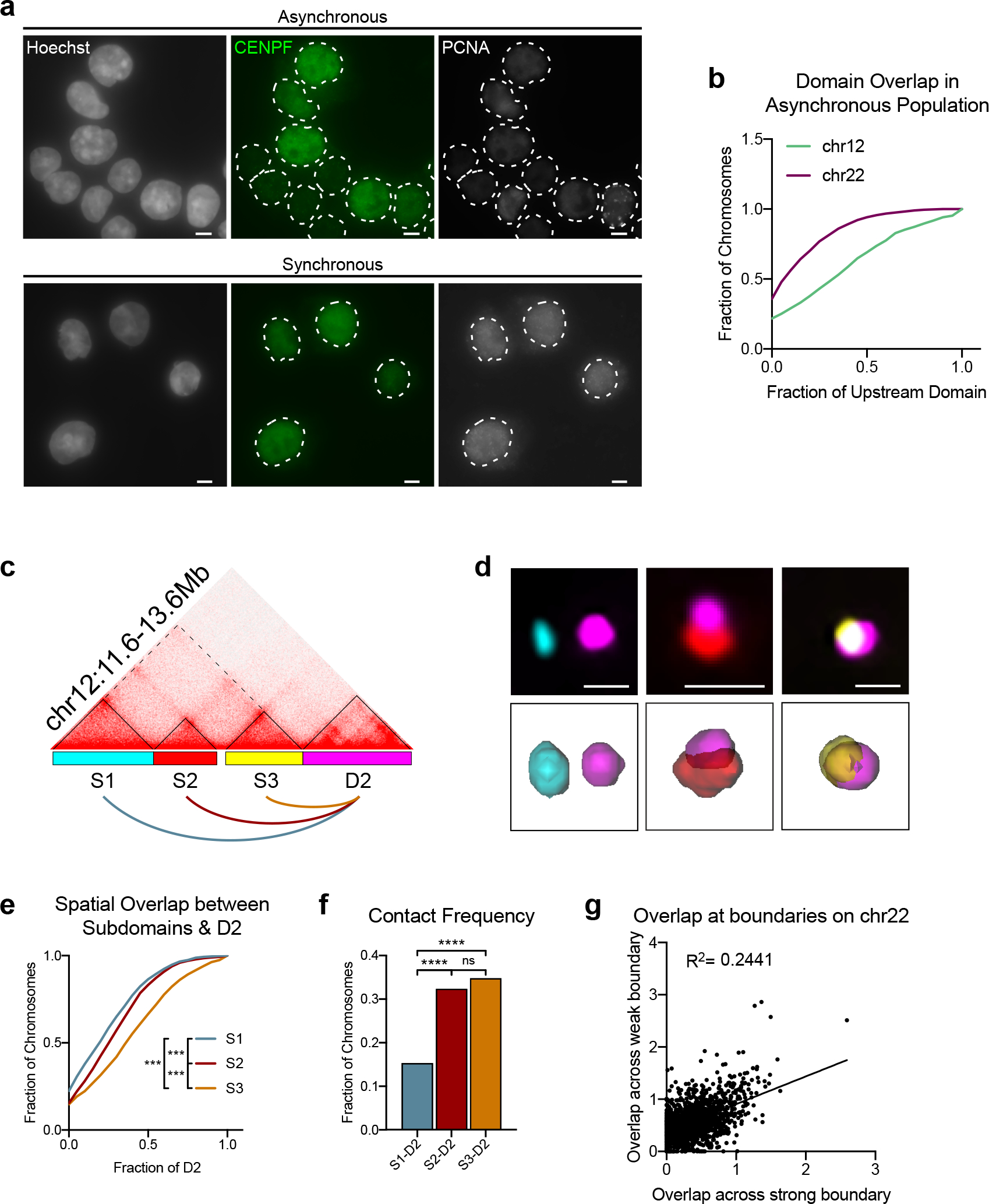
To measure the frequency and extent of interactions across architectural boundaries at the single-allele level, we designed an Oligopaint FISH-based assay that tiles probes along population-defined domains (Fig. 1a)^30–34. We applied our FISH assay in HCT-116, a human colorectal carcinoma cell line from which chromatin loops and domains have been previously defined based by high-resolution Hi-C data⁸. To rank-order boundary strengths between domains and subdomains, we determined insulation scores (IS) across the genome using the mean contact frequency with a 25-kb sliding window³⁵. Boundaries were further refined by local IS minima and co-localization of CTCF and RAD21, based on ENCODE ChIP-seq datasets³⁶.

Fig. 1. Boundary permissibility is a widespread feature of the human genome.

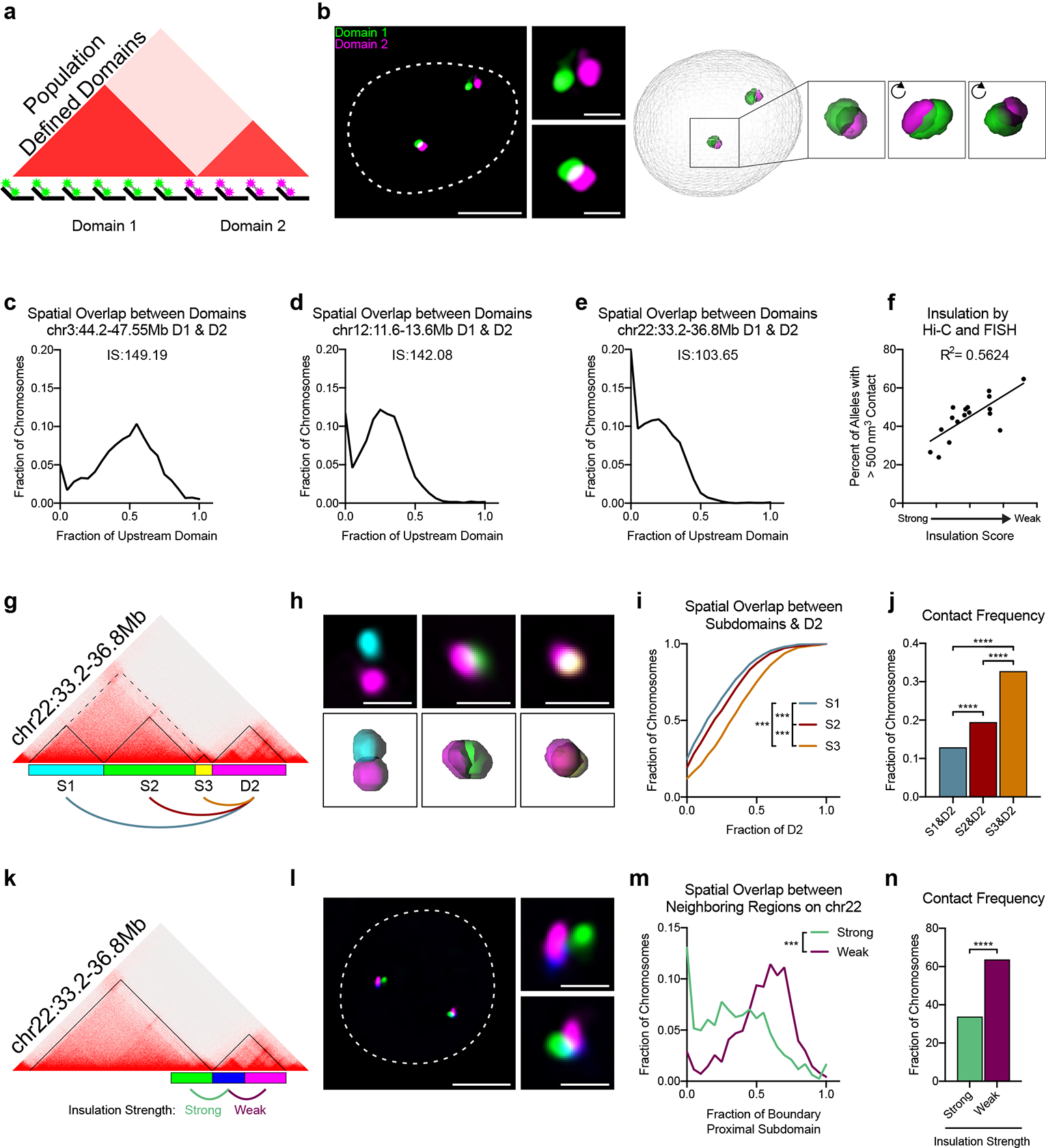
a, Oligopaint design to label two population-defined TADs. b, Representative image of neighboring domains at chr12:11.6Mb-13.6Mb with corresponding 3D image reconstruction. Dashed line represents nuclear edge. Scale bar equals 5 μm (left) or 1 μm (zoomed images, right). c, Distribution of spatial overlap between the neighboring domains (D1 & D2) at chr3:44.2–47.55Mb. Overlap normalized to the volume of the upstream domain. n = 1,642 chromosomes. IS = Insulation score of intervening boundary. d, Distribution of spatial overlap between the neighboring domains (D1 & D2) at chr12:11.6Mb-13.6Mb, normalized to the volume of the upstream domain. n = 3,986 chromosomes. e, Distribution of spatial overlap between the neighboring domains (D1 & D2) at chr22:33.2Mb-36.8Mb, normalized to the volume of the upstream domain. n = 2,835 chromosomes. f, Contact frequency of neighboring domains by FISH as a function of their boundary insulation score by Hi-C (n = 17 boundaries). Each point represents the average of two biological replicates. g, Hi-C contact matrix of chr22:33.2–36.8Mb and Oligopaint design corresponding to (h-j). h, Representative FISH image illustrating interactions between each of the three subdomains (S1-S3) and the downstream domain D2. Scale bar equals 1 μm. Corresponding 3D segmentation of FISH signals below each image. i, Cumulative distribution plot of spatial overlap between subdomains [S1 (n = 1,552); S2 (n = 1,660); S3 (n =1,822)] and D2, normalized to the volume of D2. P < 0.001, two-tailed Mann-Whitney test. j, Frequency of contact between each subdomain and D2 from data in i. Contact defined as > 500 nm³ overlap. P < 0.0001, two-tailed Fisher’s exact test. k, Hi-C contact matrix of chr22:33.2Mb-36.8Mb and Oligopaint design corresponding to (l-n). l, Representative three-color FISH image of chr22:33.2Mb-36.8Mb. Dashed line represents nuclear edge. Scale bar equals 5 μm (left) or 1 μm (zoomed images, right). m, Distribution of spatial overlap across the strong domain boundary (green, n = 1,610) and weak subdomain boundary (purple, n = 1,644). Overlap normalized to the volume of the boundary-proximal subdomain (blue probe). P < 0.001, two-tailed Mann-Whitney test. n, Frequency of contact across the strong and weak boundary from data in m. P < 0.0001, two-sided Fisher’s exact test.

We designed Oligopaint libraries targeting a total of 17 domain pairs, representing a range of gene densities, expression status, chromatin modifications, and boundary strengths across six different chromosomes (Extended Data Fig. 1 and Supplementary Table 1). Cells were synchronized in G1 to avoid heterogeneity due to the cell cycle or presence of sister chromatids (Extended Data Fig. 2a). We used custom 3D segmentation³⁷ to trace the edges of each domain signal and generate a distribution of domain volumes across a minimum of 1,500 alleles per domain pair (Fig. 1b). The overlap volume per allele was normalized to the volume of each domain to control for the varying genomic lengths at the loci tested. If population-defined domains exist as spatially separate structures, we would expect little to no overlap between adjacent domains. This was indeed the case for 2–35% of alleles across all loci tested (Fig. 1c–e and Extended Data Fig. 3a–n). Thus, the majority of alleles exhibited a wide range of overlap fractions and the amount of intermingling differed in a locus-specific manner. Similar results were also observed in asynchronous cell populations, indicating this is not a feature specific to cells in G1 (Extended Data Fig. 2b).

To compare our FISH data to that of Hi-C, we plotted the frequency of domain contact to the insulation score of their shared boundary. We find a good correlation between these two metrics (R² = 0.56; Fig. 1f), suggesting Hi-C and our FISH assay are in agreement when comparing relative contact frequencies across different boundaries. Moreover, since the insulation score of the boundary can predict contact between domains by FISH, we hypothesized the majority of interactions most likely occur near the population-defined boundary. Indeed, when we subdivided upstream domains into three subdomains anchored by CTCF/RAD21 sites, the boundary-proximal regions exhibited the most contact and overlap with the downstream domain (Fig. 1g–j; Extended Data Fig. 4c–f).

Across all loci tested, the strongest and weakest boundaries exhibited ~2-fold difference in their inter-domain contact (Fig. 1f). To measure interactions across a strong and weak boundary simultaneously, we labeled three ~500-kb regions on chromosome 22 (Fig. 1k–l). As expected, overlap across the weak subdomain boundary occurred more frequently and to a larger extent than across the stronger domain boundary (Fig. 1m–n). Specifically, we observed almost 2-fold more contact across the weak boundary as compared to the strong boundary. This is remarkably similar to the ~2-fold genome-wide average increase in intra-domain contacts recently estimated from Hi-C data³⁸. Surprisingly, we observed only a modest correlation (R² = 0.24) between domain overlap across the strong and weak boundaries on the same allele (Extended Data Fig. 2g), suggesting that interactions across each boundary occur independently from one another. Together, these data suggest that boundary permissibility is a widespread feature of the human genome but that the extent of permissibility differs in a locus-specific manner.

Variable interactions across boundaries occur independently from intra-domain compaction

Our data suggest that interactions across population-defined boundaries are frequent and extensive events. To validate our results at higher resolution and determine the impact of regional compaction on these interactions, we applied super-resolution microscopy using 3D stochastic optical reconstruction (3D-STORM) to visualize adjacent domains with < 50 nm error in their localization and < 5% error in their physical sizes³⁰. We chose two pairs of consecutive domains flanking relatively weak (IS = 142) and strong (IS = 103) boundaries located on chromosomes 12 and 22, respectively (Fig. 2a). These domain pairs were also chosen based on their differing chromatin modification landscapes (Extended Data Fig. 1). In particular, the shared boundary between the domain pair on chromosome 12 is contained within an active A compartment whereas the domain pair on chromosome 22 is mostly contained within a silent B compartment.

Fig. 2. Variable interactions across boundaries occur independently from intra-domain compaction.

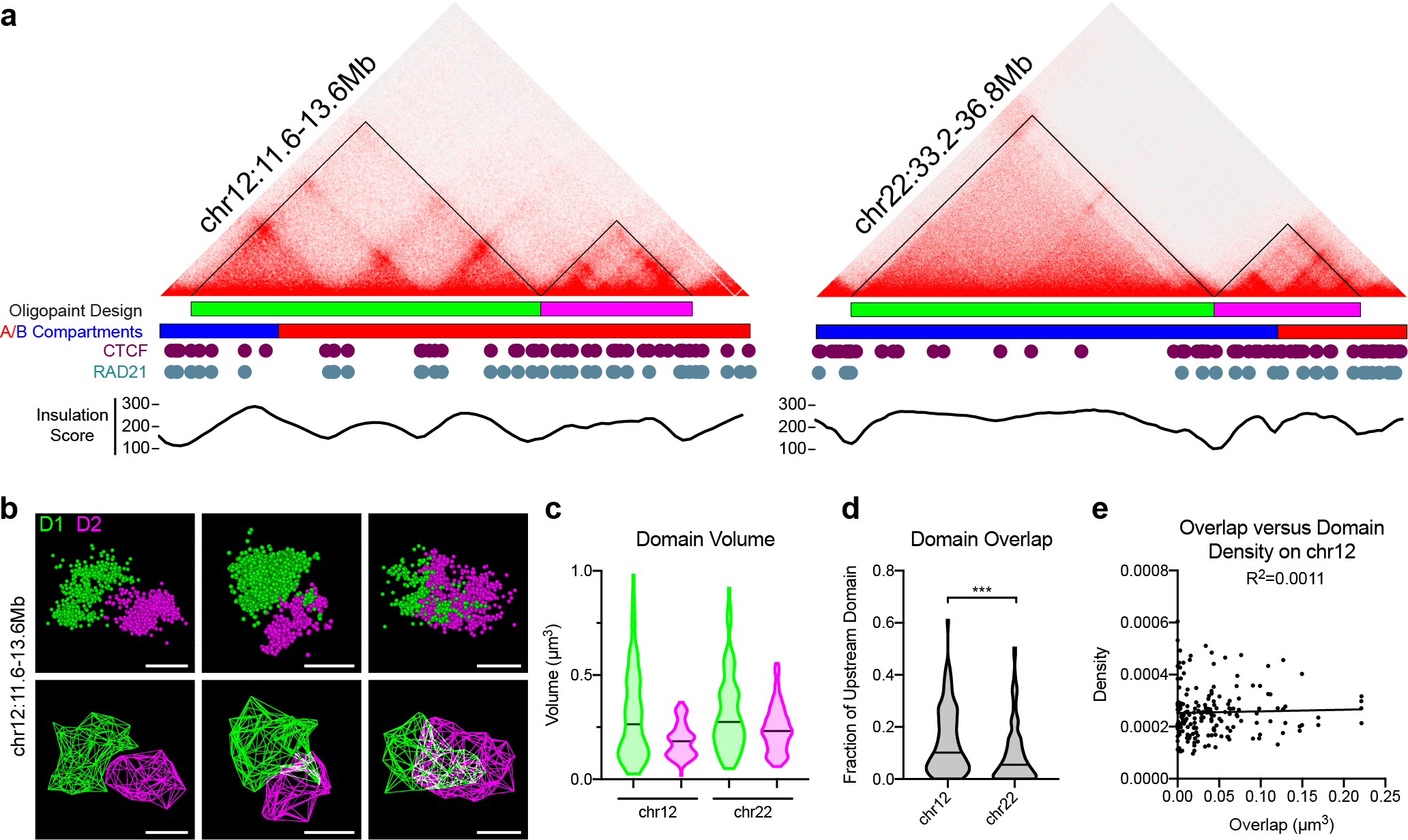
a, Hi-C contact matrices and Oligopaint probe design for neighboring domains on chromosomes 12 (left) and 22 (right), with corresponding A/B compartment designations, CTCF and RAD21 binding profiles, and Hi-C insulation scores. b, Representative 3D-STORM localizations (above) and 3D hull reconstructions (below) for neighboring domains on chr12:11.6Mb-13.6Mb. Scale bars equal 500 nm. c, Domain volume quantified from 3D-STORM images. Chr12.D1 (median = 0.2629 μm³, n = 91); Chr12.D2 (median = 0.1830 μm³, n = 91); Chr22.D1 (median = 0.2749 μm³, n = 95); Chr22.D2 (median = 0.2320 μm³, n = 95). d, Spatial overlap between neighboring domains, normalized to the volume of the upstream domain Chr12 (median = 0.1013 μm³, n = 91); Chr22 (median = 0.05466 μm³, n = 95). p < 0.001, two-tailed Mann Whitney test. e, Volume of spatial overlap between neighboring domains D1 and D2 at chr12:11.6Mb-13.6Mb (x-axis) versus the particle density of either domain (y-axis). n = 91 chromosomes.

We observed a wide diversity in the shape, volume, and particle density of each domain across the cell population (Fig. 2b–c and Extended Data Fig. 4a). While alleles within the same cell showed a moderate correlation in domain volume, no such correlation was observed between neighboring domains across the same chromosome (Extended Data Fig. 2b–e), indicating stochastic compaction rates were intrinsic to each domain.

The spatial overlap between neighboring domains recapitulated the results observed by diffraction-limited microscopy. Notably, spatially separated alleles were observed twice as frequently across the strong boundary on chromosome 22 (34%) versus the relatively weaker boundary on chromosome 12 (15%) (Fig. 2d). However, the majority of chromosomes (66–85%) at both loci showed some level of intermingling between the probed domain pairs. Neighboring domains overlapped by up to 50–61%, indicating a high level of inter-domain interactions across the cell population. Importantly, the amount of spatial overlap between neighboring domains did not correlate with the particle density of either domain (Fig. 2e and Extended Data Fig. 4f). This indicates that interactions between domains are not a direct result of regional decompaction. These results align with recent reports of heterogeneous domain intermingling^26–29, and together suggest that an independent process is driving chromatin folding in a region-specific manner.

Cohesin promotes interactions within and across domain boundaries

To test the contribution of cohesin to inter-domain interactions, we carried out an acute depletion of RAD21, a core component of the cohesin ring, via auxin-inducible degradation (AID) in HCT-116 cells³⁹. Previous work has shown that RAD21 degradation leads to a complete loss of loop domains by Hi-C (Fig. 3a)⁸, which can be attributed to a randomization of boundary positions at the single-cell level by sequential FISH²⁷. To determine if this randomization was associated with ectopic interactions across boundaries, we repeated our FISH assay in synchronized G1 cells treated with auxin for 6 hours. This treatment resulted in a > 95% reduction in chromatin-bound RAD21 levels (Extended Data Fig. 5a–c).

Fig. 3. Cohesin promotes interactions within and across domain boundaries.

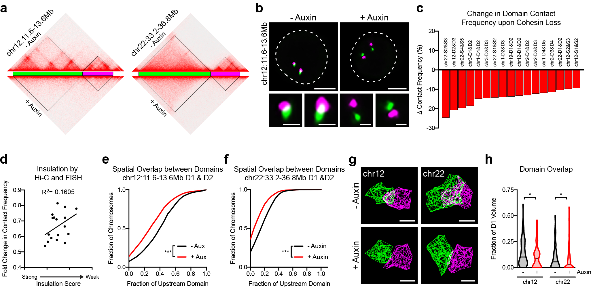
a, Hi-C contact matrices and Oligopaint probe design of chr12:11.6Mb-13.6Mb and chr22:33.2–36.8Mb in HCT-116-RAD21-AID cells prior to or after 6 hours of auxin treatment. b, Representative FISH images of neighboring domains across chr12:11.6Mb-13.6Mb prior to and after auxin treatment. Dashed lines represent nuclear edges. Scale bar equals 5 μm (left) or 1 μm (zoomed images, below). c, Locus-specific differences in the percentage of domain pairs in contact following auxin treatment. Each bar represents an average of two biological replicates. d, Fold-change in contact frequency between neighboring domains following auxin treatment versus the insulation score of their intervening boundary. Each point represents an average of two biological replicates. n = 17 boundaries. e, Cumulative distribution of overlap between the neighboring domains at chr12:11.6–13.6Mb prior to (n = 1,625) and after auxin treatment (n = 1,607). Overlap normalized to the volume of the upstream domain. P < 0.001, two-tailed Mann-Whitney test. f, Cumulative distribution of overlap between the neighboring domains at chr22:33.2–36.8Mb prior to (n = 2,835) and after auxin treatment (n = 2,803). Overlap normalized to the volume of the upstream domain. P < 0.001, two-tailed Mann-Whitney test. g, Representative 3D hull reconstructions of 3D-STORM localizations for neighboring domains on chr12:11.6–13.6Mb. Scale bar equals 500 nm. h, Spatial overlap between domains on chr12:11.6–13.6Mb and chr22:33.2–36.8Mb, normalized to volume of the upstream domain. P = 0.044 for domains on chromosome 12 (prior to auxin: median = 0.1013 μm³, n = 91; after auxin: median = 0.08967 μm³, n = 76); P = 0.029 for domains on chromosome 22 (prior to auxin median = 0. 05466 μm³, n = 95; after auxin median = 0. 03250 μm³, n = 105), two-tailed Mann-Whitney test.

Despite the loss of recurrent boundaries by Hi-C and FISH, all 17 domain pairs we assayed exhibited reduced contact frequencies following RAD21 degradation (Fig. 3b–c). Although cohesin loss reduced contact between some domain pairs more than others, these locus-specific differences did not seem to reflect the size or chromatin type of domain pair being tested. Instead, there was a moderate but significant correlation between the fold change in contact frequency and the boundary strength prior to treatment (Fig. 3d). While this cannot fully explain the locus-specific differences in effect size, it does suggest that weaker boundaries were more sensitive to cohesin loss. When overlap was observed in absence of cohesin, domains intermixed significantly less at all loci tested (P < 0.001; Fig. 3e–f and Extended Data Fig. 6a–u). We validated these findings using 3D-STORM, which revealed an increase in spatial separation between domains following cohesin loss across both a strong and weak boundary (Fig. 3g–h and Extended Data Fig. 7a–b). Importantly, the volume and single-molecule particle density of each genomic region being probed did not increase following cohesin loss at any of the four domains assayed (Extended Data Fig. 7c–d). Taken together, this suggests that while cohesin is not responsible for compacting chromatin at these loci, it does promote intermingling within and between their population-defined domains.

WAPL and CTCF restrict cohesin-dependent interactions across domain boundaries

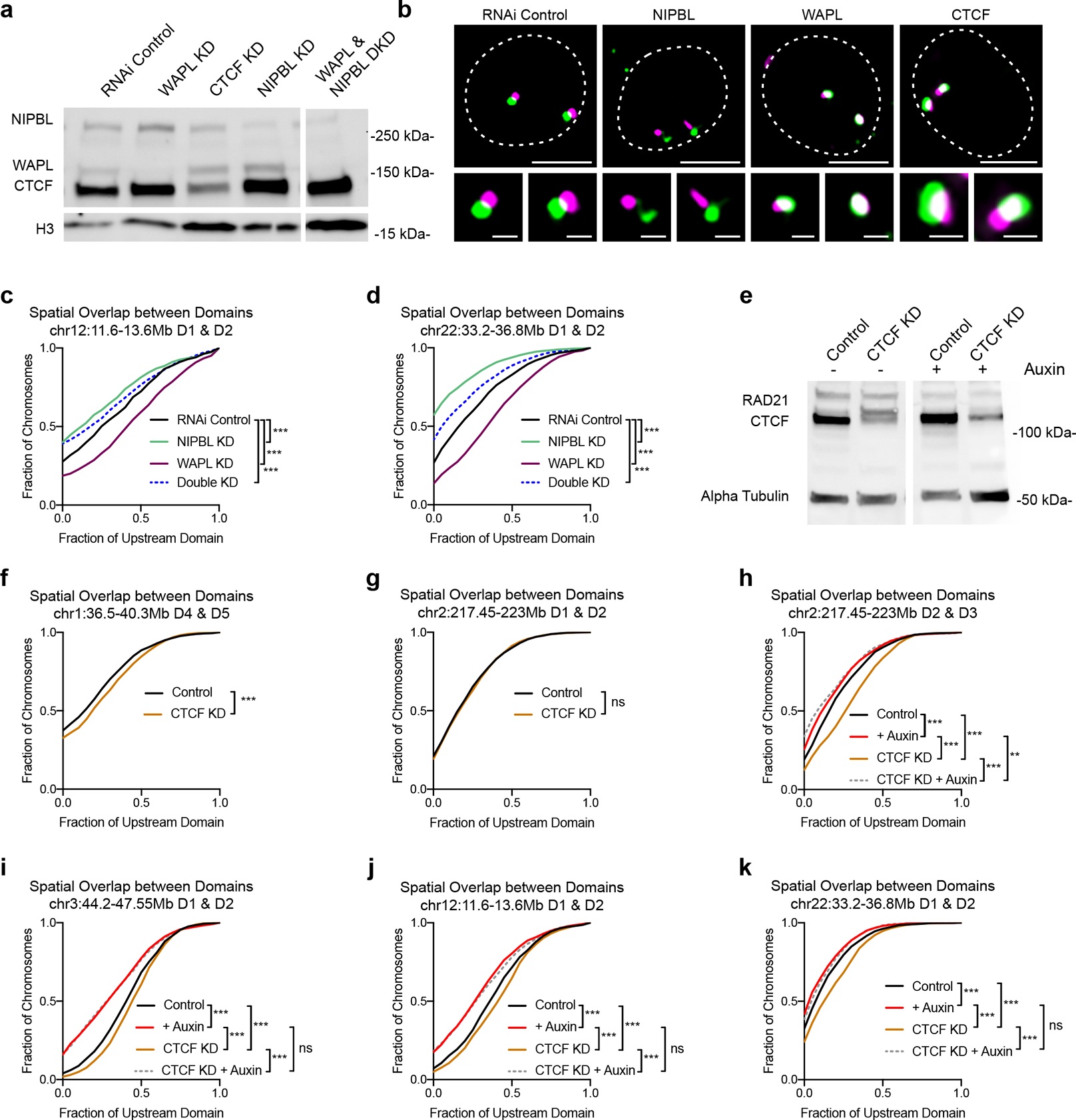
Loop extrusion models would predict that altering the processivity of cohesin could affect the extent of inter-domain interactions. Therefore, we next depleted regulators of cohesin to determine their effect on chromatin intermingling across domain boundaries. Cohesin is loaded onto chromatin by NIPBL, whereas the negative regulator of cohesin, WAPL, opens the cohesin ring to release it from DNA⁴⁰. We depleted NIPBL and WAPL using RNAi in HCT-116 cells to decrease and increase cohesin occupancy, respectively, and then measured the overlap between neighboring domains at two loci by FISH (Fig. 4a and Extended Data Fig. 8a–b). NIPBL-depleted chromatin showed significantly (P < 0.001) less contact and more spatial separation between domains, similar to RAD21 degradation. NIPBL knockdown also showed a more severe domain separation across the weak boundary on chromosome 12 as compared to the strong boundary on chromosome 22. In contrast, WAPL-depleted chromatin showed significantly more contact and greater overlap (P < 0.001) between the domains and to a similar extent at both loci (Fig. 4b–d). Double knockdown of NIPBL and WAPL phenocopied NIPBL depletion alone, indicating the increase in overlap was cohesin-dependent (Extended Data Fig. 8c–d).

Fig. 4: WAPL and CTCF restrict cohesin-dependent interactions across domain boundaries.

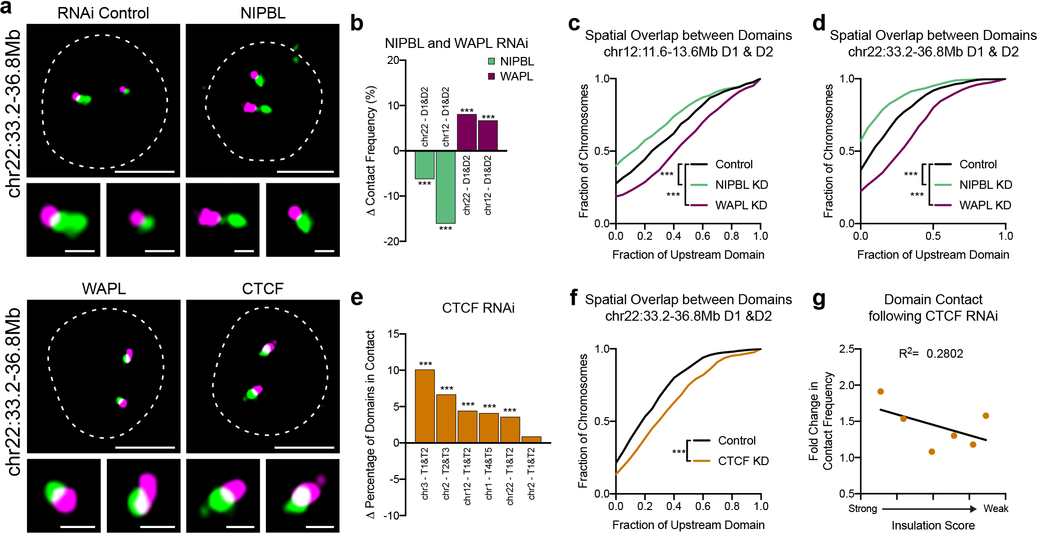
a, Representative FISH images of neighboring domains on chr22:33.2–36.8Mb in RNAi control, NIPBL-, WAPL-, or CTCF-depleted HCT-116 cells. Dashed lines represent nuclear edges. Scale bar equals 5 μm (left) or 1 μm (zoomed images, below). b, Difference in the percentage of domain pairs in contact following depletion of NIPBL or WAPL. Each bar represents an average of three biological replicates. P < 0.001, two-tailed Mann-Whitney test. c, Cumulative frequency distribution of spatial overlap between neighboring domains on chr12:11.6Mb-13.6Mb in control (n = 643 chromosomes), NIPBL- (n = 636) or WAPL-depleted (n = 819) cells. Overlap normalized to the volume of the upstream domain. P < 0.001, two-tailed Mann-Whitney test. d, Cumulative frequency distribution of spatial overlap between neighboring domains on chr22:33.2–36.8Mb in control (n = 819 chromosomes), NIPBL- (n = 573) or WAPL-depleted (n = 877) cells. Overlap normalized to the volume of the upstream domain. P < 0.001, two-tailed Mann-Whitney test. e, Difference in the percentage of domain pairs in contact following depletion of CTCF. Each bar represents average of three biological replicates. P < 0.001, two-tailed Mann-Whitney test. f, Cumulative frequency distribution of spatial overlap between neighboring domains on chr22:33.2Mb-36.8Mb in control (n = 449 chromosomes) or CTCF-depleted (n = 332) cells. Overlap normalized to the volume of the upstream domain. P < 0.001, two-tailed Mann-Whitney test. g, Fold-change in contact frequency between neighboring domains following depletion of CTCF versus the insulation score of their intervening boundaries. Each point represents an average of two biological replicates. n = 6 boundaries.

We next depleted the insulator protein CTCF, which similarly to cohesin, is necessary for loops and domains at the population-average level²³. In contrast to cohesin loss, however, we observed significantly increased contact and spatial overlap at 5 out of 6 domain pairs tested (P < 0.001), similar to WAPL depletion (Fig. 4a,e–f and Extended Data Fig. 8e–k). Therefore, depletion of cohesin and CTCF show opposite effects on inter-domain interactions by FISH, despite their comparable loss of population-defined domains by Hi-C^8,23,24. Additionally, in contrast to cohesin, the fold-change in contact between neighboring domains was negatively correlated with the insulation score at the boundary prior to RNAi (R² = 0.28), such that stronger boundaries were more dependent on CTCF (Fig. 4g). Note that all domain pairs tested had a CTCF site at their shared boundary (Extended Data Fig. 1). Auxin-mediated depletion of RAD21 following CTCF knockdown phenocopied RAD21 depletion alone, indicating the increase in overlap was cohesin-dependent (Extended Data Fig. 8f,h–k). Taken together, these results indicate that CTCF and WAPL restrict but do not eliminate cohesin-dependent interactions across population-defined boundaries.

Cohesin alters the topological context of boundary-proximal genes

Chromatin loops and domains are implicated in the regulation of gene expression and previous work using nascent RNA-sequencing revealed 4,196 genes to be differentially expressed in HCT-116 cells following RAD21 degradation, albeit with relatively modest changes⁸ (Fig. 5a). Several differentially expressed genes (DEGs) are associated with RAD21/CTCF binding sites and are thus in close proximity to domain boundaries. Given that domains are less likely to interact in the absence of cohesin, we reexamined the spatial position of these genes relative to their neighboring population-defined domains in control and RAD21-depleted cells. This analysis was conducted for two DEGs, CREBL2 and MCM5, whose transcription start sites (TSSs) are within 125 and 50 kb of a domain boundary, respectively (Fig. 5b and Extended Data Fig. 9a).

Fig. 5. Cohesin alters the topological context of boundary-proximal genes.

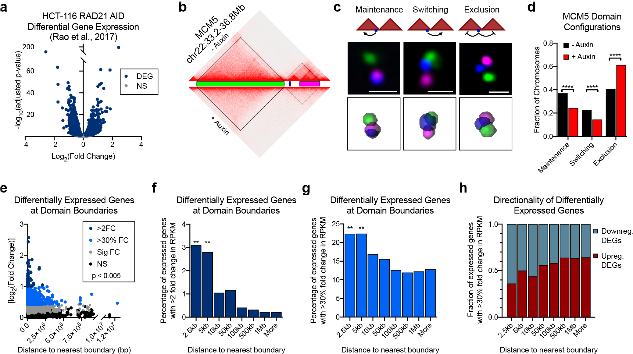
a, The log₂(fold-change) versus significance of differentially expressed genes (DEGs) by PRO-seq data reported in Rao et al.⁸. Differentially expressed genes in blue; expressed genes that are not significant (NS) in grey. b, Hi-C contact matrix for chr22:33.2–36.8Mb and corresponding Oligopaint design for (c-d). Blue represents the boundary proximal gene MCM5. c, Cartoon depicting three possible interactions between boundary-proximal genes and their neighboring domains: domain maintenance, switching, and exclusion (top). Representative images of three-color FISH to the chr22:33.2–36.8Mb locus illustrating the three domain configurations (middle); scale bar equals 1 μm. Corresponding 3D segmentation of FISH signals below each image. d, Frequencies of domain configurations at chr22:33.2–36.8Mb prior to (n = 919) or after auxin treatment (n = 863). P < 0.0001, two-sided Fisher’s exact test. e, [log₂(fold-change)] of differentially expressed genes (DEGs) versus the distance between their TSS and the center of the nearest domain boundary. P = 0.0025, Spearman’s correlation. f, Percentage of expressed genes at binned distances from the center of the nearest domain boundary that are differentially expressed by > 2 log₂(fold-change) upon auxin treatment in the HCT-116 cells. P < 0.001, two-sided Fisher’s exact test. g, Percentage of expressed genes at binned distances from the center of the nearest domain boundary that are differentially expressed by > 30% fold change upon auxin treatment in the HCT-116 cells. P < 0.001, two-sided Fisher’s exact test. h, Fraction of genes that are up- or down-regulated following auxin treatment in HCT-116 cells at binned distances from the nearest domain boundary.

We defined four topological configurations based on the position of the gene relative to either domain: 1) the gene interacts with its expected contact domain (domain maintenance), 2) the gene interacts with the neighboring domain (domain switching), 3) the gene no longer interacts with either domain (domain exclusion), or 4) the gene interacts simultaneously with both domains (domain sharing) (Fig. 5c). Although all four configurations occurred throughout the cell population, < 1% of cells exhibited a domain sharing configuration in which the gene interacted with both domains simultaneously. This indicates that stochastic domain intermingling is not due to complete domain merging but instead arises from the asymmetric incorporation of boundary-proximal chromatin with its neighboring regions, consistent with a shifting boundary position across individual cells. Indeed, the MCM5 gene interacted with the upstream portion of its own domain in 37% of alleles and interacted exclusively with the neighboring domain at a similar frequency (22%; Fig. 5d). Most commonly, the gene was spatially excluded from either domain (40%). Similar results were obtained for the boundary-proximal DEG CREBL2 on chromosome 12 (Extended Data Fig. 9b–c). These results further highlight the variable nature of domain boundaries and suggest that genes near boundaries are frequently located outside of their expected population-defined topological context.

Following auxin treatment to deplete RAD21, the MCM5 locus was more frequently excluded from either domain (61% of alleles; Fig. 5d). A similar increase in spatial exclusion was found for CREBL2 (Extended Data Fig. 9c). At both loci, this was accompanied by a significant reduction in both domain maintenance and switching. Therefore, in the absence of cohesin, domain separation preferentially induces increased exclusion of these boundary-proximal genes from neighboring domains in a fraction of cells.

Boundary proximity correlates with gene expression changes following cohesin dysfunction

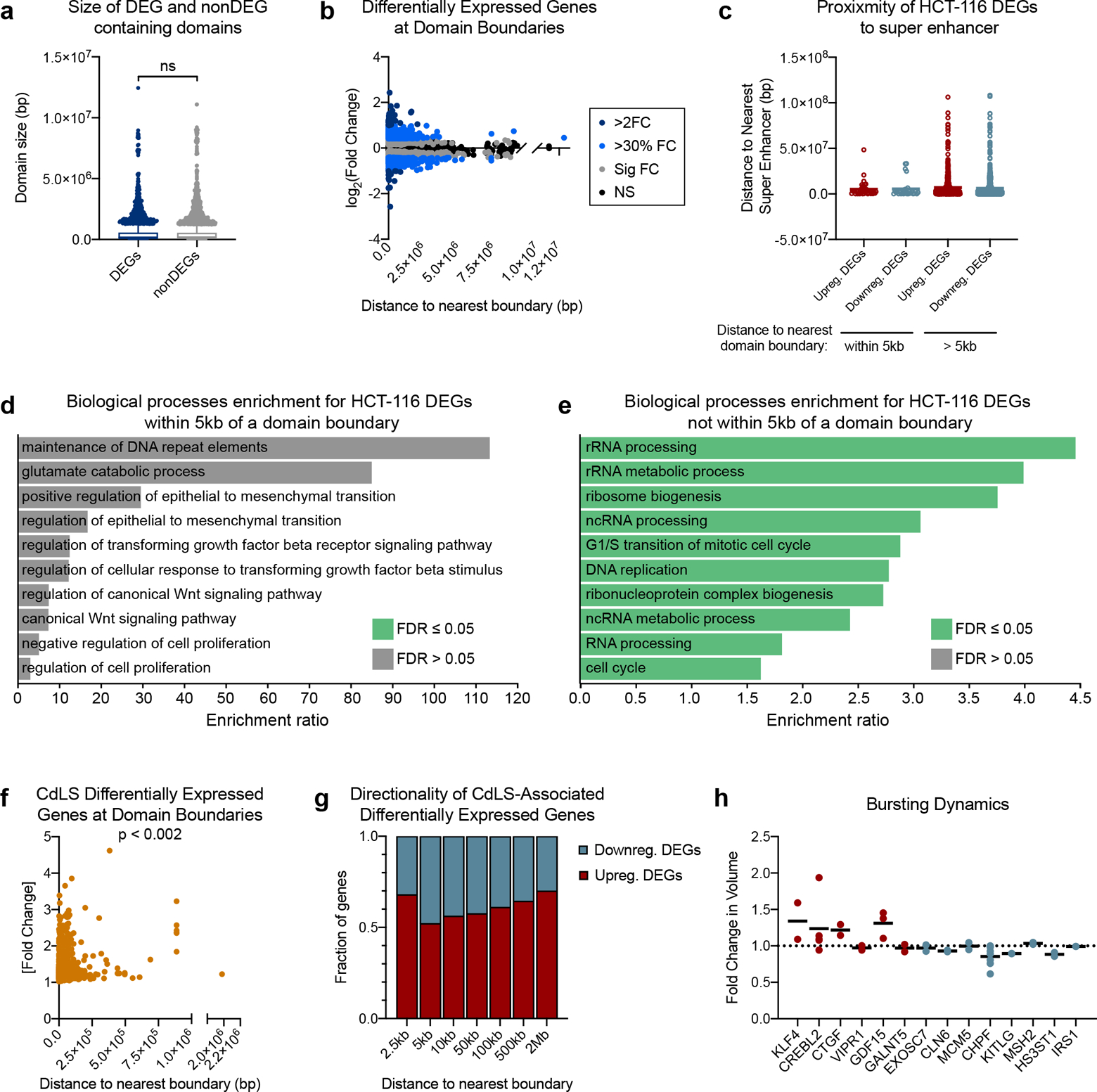
Nearly all regulatory elements and their target promoters are mapped within the same population-defined domain^11–14. We therefore reasoned that the expression of genes near boundaries may be especially sensitive to cohesin loss due to increased exclusion from their neighboring regulatory domains. We plotted the distance between the TSS of each expressed gene and the nearest domain boundary as a function of their log₂ fold-change in expression using data from Rao et al.⁸. Overall, TSSs of expressed genes were found at varying distances from domain boundaries and spanned the full length of the domain size range (Fig. 5e). However, DEGs with a higher fold-change in expression were enriched near domain boundaries as compared to lower fold change or unchanged genes (P < 0.005; Fig. 5e). For example, most DEGs with > 2-fold change in expression following cohesin loss were located within 50 kb of a domain boundary, despite an average domain size of ~350 kb. Importantly, there was no difference in the size of domains harboring either DEGs or nonDEGs (Extended Data Fig. 10a). To control for the high gene density near domain boundaries, we calculated the percentage of all expressed genes in HCT-116 cells with > 2-fold change in expression at stratified distances from domain boundaries. We found a significant enrichment of DEGs within 2.5 and 5.0 kb of a domain boundary (Fig. 5f). We note a similar enrichment for genes with > 30% fold-change following cohesin degradation (Fig. 5g). In total, 42% of expressed genes within 5 kb of a domain boundary are differentially regulated following depletion of RAD21 with nearly equal representation of upregulated and downregulated genes (Fig. 5h and Extended Data Fig. 10b).

Interestingly, while DEGs are also nonrandomly close to super-enhancers as previously reported⁸, we found no correlation between the fold-change in expression and distance to nearest super-enhancer (Extended Data Fig. 10c). Boundary-proximal DEGs also show no enrichment for specific biological processes or pathways (Extended Data Fig. 10d–e). Only 7% of DEGs within 5 kb of a domain boundary are classified as housekeeping genes⁴¹, suggesting the majority of boundary-proximal DEGs are likely cell-type-specific.

To determine if this is a general signature of cohesin loss, we also analyzed data from lymphoblastoid cells (LCLs) derived from patients with NIPBL mutations, which causes a rare developmental disorder called Cornelia de Lange syndrome (CdLS)^42,43. Previous studies have found decreased chromatin-bound RAD21 levels and a total of 1,500 genes that are recurrently differentially expressed across patient-derived LCLs⁴³. Similar to DEGs following RAD21 degradation in HCT-116 cells, the extent of misexpression for CdLS-associated DEGs is correlated to their distance from a boundary (Extended Data Fig. 10f–g). Together, this indicates that genes at the boundaries of domains are more likely to be differentially expressed and to a larger extent following cohesin dysfunction.

Cohesin alters the transcriptional bursting frequency of boundary-proximal genes

Cohesin loss may alter transcription of boundary-proximal genes either by influencing how frequently the gene is transcribed (transcription burst frequency) or how much PolII is loaded during each burst (burst size). To determine which level of transcriptional regulation cohesin functions at, we performed intronic RNA FISH to six upregulated and eight downregulated boundary-proximal genes (Fig. 6a). All 14 genes exhibited bursty transcription by RNA FISH, calculated by the fraction of active alleles, and are positioned between 363 bp and 125 kb of a domain boundary (Fig. 6b–c).

Fig. 6. Cohesin alters the transcriptional bursting frequency of boundary-proximal genes.

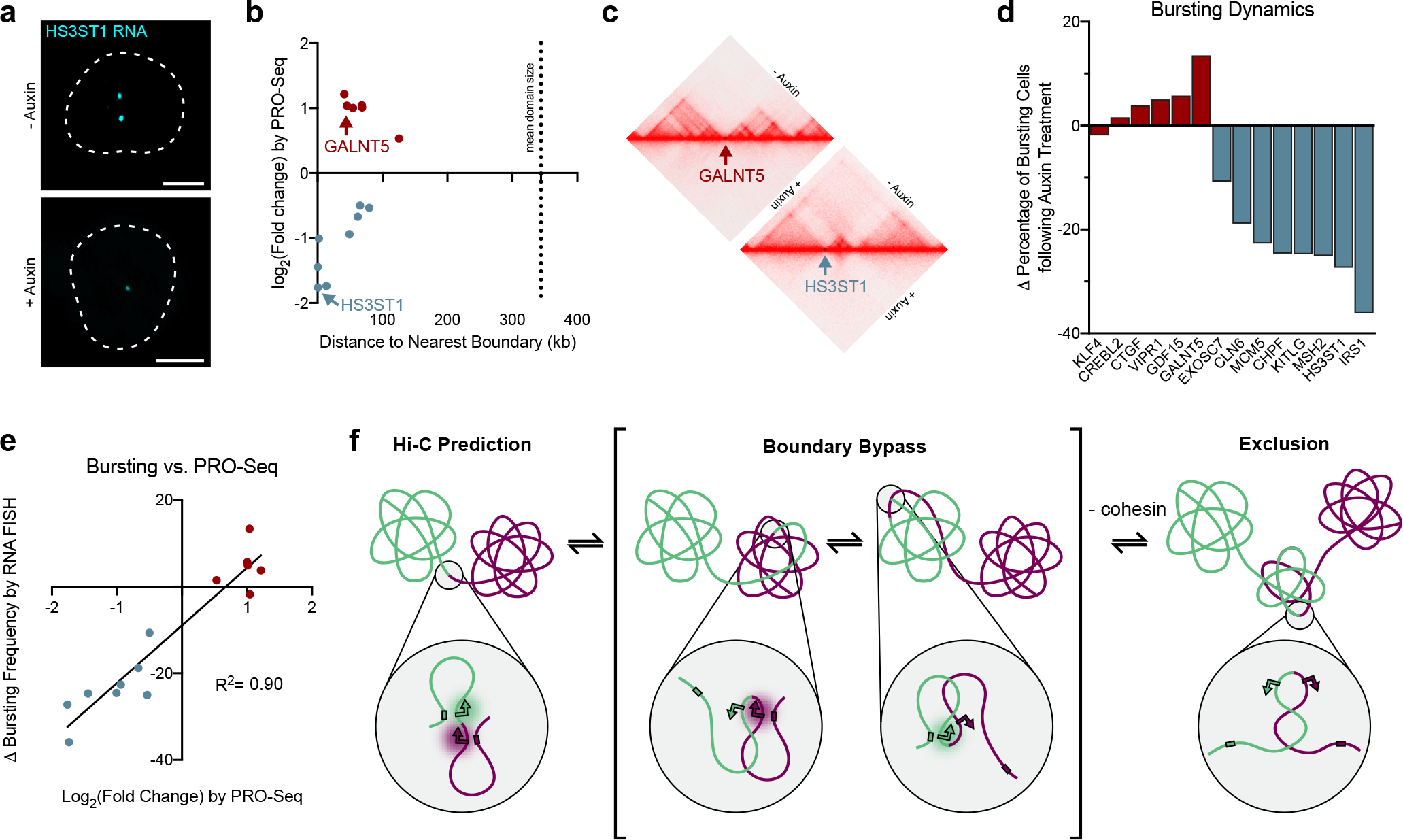
a, Representative images of intronic RNA FISH to the HS3ST1 transcript before or after auxin treatment. Dashed lines represent nuclear edges. Scale bar equals 5 μm. b, Scatterplot indicating the gene expression changes previously reported by PRO-seq⁸ and distance to nearest boundary for genes assayed by RNA FISH. The mean domain size denoted by a hashed line is 343.9 kb. c, Hi-C contact matrices of the loci surrounding GALNT5 and HS3ST1. Hi-C maps shown for HCT-116 cells before or after auxin treatment to degrade RAD21.

d, Change in bursting frequency of each gene following auxin treatment by intronic RNA FISH. n > 227 chromosomes. Average of 3 biological replicates per gene. e, Change in gene expression previously reported by PRO-seq⁸ versus change in bursting frequency detected by intronic RNA FISH (R² = 0.9047, two-sided Pearson correlation). P < 0.0001, n = 14 boundaries. f, Model of single-cell variability in domain formation. Two architectural domains are depicted in green and magenta, with arrows indicating a boundary-proximal promoter in each domain. Colored rectangles represent the appropriate enhancer for each gene. Cohesin promotes variable boundary bypass such that the boundary-proximal chromatin is asymmetrically incorporated with the neighboring domains in a large fraction of cells. The boundary-proximal promoters thus alternate their contact with regulatory elements in their respective domains, which can result in a transcriptional burst. In the absence of cohesin, the boundary-proximal region is more often excluded from either domain such that promoters in this region are less frequently exposed to their regulatory elements. This could explain both downregulation and upregulation of DEGs if a boundary-proximal gene were looped out away from a distal enhancer or silencer, respectively.

With the exception of KLF4, we observed altered bursting frequency in all genes following RAD21 degradation with a large range of effect sizes (Fig. 6d). A few upregulated DEGs, including KLF4, exhibited moderate increases in burst size (Extended Data Fig. 10). In contrast, all eight downregulated genes exhibited significant decreases in burst frequency, but the burst size was largely unaffected. Overall, the shifts in bursting frequency across all 14 DEGs were consistent with their directionality and relative changes in expression as shown by PRO-seq with a correlation of R² = 0.90 (Fig. 6e). Based on these data, we propose that cohesin promotes proper gene expression at the level of transcriptional bursting frequency at genes near domain boundaries.

Discussion

Subsequent to their discovery, early models suggested that TADs are functional regulons, which spatially separate into 3D structures to insulate gene regulation. Using Oligopaint FISH technology to precisely target population-defined domains, our data add to an emerging theme from recent single-cell based assays that genome packaging is extremely dynamic and heterogeneous across a cell population^{27–29,44,45}. We find that, on average, ~45% of alleles show some degree of intermingling between adjacent population-defined domains. We also show that interactions are enriched near their shared boundaries with ~2-fold less contact across the strongest versus weakest elements (Fig. 1f). Using three-color FISH, we show that boundary-proximal chromatin is asymmetrically incorporated with neighboring domains. Thus, our data are consistent with variable boundary positions between population-defined domains as reported by Bintu et al.²⁷ (Fig. 6f). The simplicity of our domain FISH assay allowed us to extend this conclusion to many loci of different chromatin types, suggesting boundaries flanked by domains of the same or different compartments are similarly permissible. While we cannot rule out the possibility that some boundaries in the genome remain invariable, our data suggest that interactions across population-defined boundaries are a widespread feature of the human genome.

The loop extrusion model, in which cohesin complexes extrude DNA until halted by a convergent pair of CTCF motifs, has been proposed to explain the formation of loops and domains at the population average level^17,18. Indeed, we find that cohesin promotes intermingling within and between population-defined domains in single cells as has been predicted from polymer simulations⁴⁶. We also find increased interactions between domains following WAPL or CTCF knockdown, consistent with their role in restricting cohesin-based chromatin extrusion^4,47. Combined with the dynamic nature of cohesin and CTCF binding^4,8, we propose that cohesin-mediated stochastic boundary bypass toggles boundary incorporation between neighboring domains across a single cell cycle (Fig. 6f).

Finally, we consider our results in the context of gene expression and the role TADs are proposed to play in transcriptional regulation. In particular, if population-defined domains contain the appropriate regulatory elements for the genes that lie within, why would cells permit such variability in boundary positions? This might be a consequence of cohesin processivity and CTCF binding dynamics, which, based on recent estimates⁴, are too rapid to facilitate such precise and prolonged chromatin interactions. Alternatively, shifting boundary positions may offer advantages over an invariable system. We identified a signature of RAD21 loss in which genes near population-defined boundaries are more likely to be misexpressed and to a larger extent. We find a similar signature in cells derived from NIPBL-deficient CdLS patients, suggesting this is a general feature of cohesin dysfunction.

It is not entirely clear why boundary-proximal genes would be more sensitive to cohesin loss. However, cohesin-mediated incorporation of boundary-proximal chromatin with either of its neighboring domains would ensure a high probability of contact between all portions of a regulatory domain over time. This would be especially important for boundary-proximal genes, as these genes may need to travel up to twice the maximum distance a gene near the TAD center would to contact a distal regulatory element. Indeed, increased exclusion of these genes from neighboring domains following cohesin loss could explain both downregulation and upregulation of DEGs if a boundary-proximal gene were looped out away from a distal enhancer or silencer, respectively (Fig. 6f). Excitingly, a recent preprint reported that long-range enhancer-promoter interactions anchored at domain boundaries are preferentially dissolved in the absence of cohesin, which is accompanied by decreased nascent transcription at these loci⁴⁸. This is supported by our finding that cohesin regulates genes at the level of transcriptional bursting, which may be attributed to altered enhancer-promoter engagement⁴⁹. Thus, our results suggest a paradigm in which cohesin dynamically bypasses boundaries to create stochastic domain structures that help regulate gene expression.

Methods

TopDom insulation score calculation

Published Hi-C data were downloaded from GEO database (GSE104334, GSE63525) and the 25-kb window contact matrix was extracted with the Juicebox tools (v1.9.8, “dump observed KR”). TopDom (v0.0.2) was then used to identify topological domains and define insulation scores from the contact matrix, with the optimization parameter window.size set to be 10 (including data within 10 windows when computing local topological domains). Domains were further processed to include only those between 250 kb and 2 Mb in size.

Compartment analysis

To designate compartments in the HCT-116-RAD21-AID cell line, we determined eigenvectors from Hi-C data reported in Rao et al.⁸. We applied the eigenvector feature annotation package included in the Juicer software (https://github.com/aidenlab/juicer/wiki/Eigenvector) with KR normalization at 500-kb resolution⁵⁰. While the sign of the eigenvector typically reflects the A or B compartment designation, we further confirmed compartment designations by comparing the eigenvector coordinates with ChIP-seq data for various histone modifications marking active and inactive chromatin from previously published data⁸ (Extended Data Fig. 1).

Oligopaint design and synthesis

To label domains in the HCT-116-RAD21-AID cell line, we first applied the TopDom TAD algorithm to Hi-C data reported in Rao et al.⁸ to define insulation scores. We then identified RAD21 and CTCF colocalized sites at the boundaries between domains from ChIP-seq data available on ENCODE (ENCSR000BSB and ENCSR000DTO, respectively). We defined the domain and sub-domain boundary coordinates by the center of the corresponding RAD21 ChIP-seq peak. We then applied the OligoMiner design pipeline to design DNA FISH probes to the coordinates found in Supplementary Table 1³². Oligopaints were designed to have either 42 or 80 bases of homology with an average of five probes per kb and were purchased from CustomArray (42-mers) or Twist Bioscience (80-mers). Additional bridge probes were designed to the sub-domains and boundary-proximal genes to amplify their signal³⁰. Oligopaints were synthesized as previously described^51,52.

Cell culture

HCT-116-RAD21-AID cells were obtained from Natsume et al.³⁹. The cells were cultured in McCoy’s 5A medium supplemented with 10% FBS, 2 mM L-glutamine, 100 U/ml penicillin, and 100 μg/ml streptomycin at 37°C with 5% CO₂. Cells were selected with 100 μg/ml G418 and 100 μg/ml HygroGold prior to experiments.

To avoid heterogeneity due to cell cycle, HCT-116-RAD21-AID cells were synchronized at the G1/S transition. First, to arrest cells in the S-phase, cells were grown in medium supplemented with 2 mM thymidine (Sigma-Aldrich T1895) for 12 hours. Cells were then resuspended in medium and allowed to grow for 12 hours to exit S-phase. To arrest at the G1/S transition, we grew cells in medium supplemented 400 μM mimosine (Sigma-Aldrich M025) for 12 hours. Lastly, we replaced medium with either 400 μM mimosine + 500 μM indole-3-acetic acid (auxin; Sigma-Aldrich I5148)-supplemented medium to degrade RAD21 or 400 μM mimosine-supplemented medium alone as an untreated control; cells were incubated with or without auxin for 6 hours then harvested for experiments. Synchronization was confirmed by IF (Extended Data Fig. 2a).

RNAi

HCT-116 cells were cultured in McCoy’s 5A medium supplemented with 10% FBS, 2 mM L-glutamine, 100 U/ml penicillin, and 100 μg/ml streptomycin at 37°C with 5% CO₂. The following siRNAs (Dharmacon) were used: Non-targeting control, NIPBL, WAPL, CTCF. siRNA sequences can be found in Supplementary Table 2. Duplex siRNA were incubated for 20 minutes at room temperature with RNAiMAX transfection reagent (Thermo Fisher) in Opti-MEM reduced serum medium (Thermo Fisher) and seeded into wells. HCT-116 were trypsinized and resuspended in antibiotic-free medium, then plated with medium containing siRNA for a final siRNA concentration of 50 nM (non-targeting control, NIPBL, or WAPL) or 150 nM (CTCF). For CTCF knockdowns, cells were retreated with 150nM CTCF siRNAs 24 hours after initial treatment. After 72 h (NIPBL, WAPL, non-targeting control) or 96 h from the initial RNAi treatment (CTCF), cells were harvested for experiments. For the CTCF and RAD21 double-knockdown experiments, cells were grown in medium supplemented with 500 μM indole-3-acetic acid (auxin; Sigma-Aldrich I5148) for 6 hours following RNAi treatments, and then harvested for experiments.

DNA fluorescence in situ hybridization (FISH)

Cells were settled on poly-L-lysine-treated glass slides for 2 hours, or uncoated high-precision 22 × 22 mm coverslips for 6 hours. Cells were then fixed to the slide or coverslip for 10 minutes with 4% formaldehyde in PBS with 0.1% Tween 20, followed by three washes in PBS for 5 minutes each. Slides and coverslips were stored in PBS at 4°C until use.

For experiments imaged by widefield microscopy, FISH was performed on slides. Slides were warmed to room temperature (RT) in PBS for 10 minutes. Cells were permeabilized in 0.5% Triton-PBS for 15 minutes. Cells were then dehydrated in an ethanol row, consisting of 2 minute incubations in 70%, 90%, and 100% ethanol consecutively. The slides were then allowed to dry for about 2 minutes at room temperature. Slides were incubated 5 minutes each in 2× SSCT (0.3 M NaCl, 0.03 M sodium citrate, 0.1% Tween 20) and 2× SSCT/50% formamide at room temperature, followed by a 1 hour incubation in 2× SSCT/50% formamide at 37°C. Hybridization buffer containing primary Oligopaint probes, hybridization buffer (10% dextran sulfate/2× SSCT/50% formamide/4% polyvinylsulfonic acid (PVSA)), 5.6 mM dNTPs, and 10 μg RNase A was added to slides, covered with coverslip, and sealed with rubber cement. Fifty pmol of probe was used per 25 μl hybridization buffer. Slides were then denatured on a heat block in a water bath set to 80°C for 30 minutes, then transferred to a humidified chamber and incubated overnight at 37°C. The following day, coverslips were removed and slides were washed in 2× SSCT at 60°C for 15 minutes, 2× SSCT at RT for 10 minutes, and 0.2× SSC at RT for 10 minutes. Next, hybridization buffer (10% dextran sulfate/2× SSCT/10% formamide/4% polyvinylsulfonic acid (PVSA)) containing secondary probes conjugated to fluorophores (10 pmol/25 μl buffer) was added to slides, covered with coverslip, and sealed with rubber cement. Slides were placed in humidified chamber and incubated 2 hours at RT. Slides were washed in 2× SSCT at 60°C for 15 minutes, 2× SSCT at RT for 10 minutes, and 0.2× SSC at RT for 10 minutes. To stain DNA, slides were washed with Hoechst (1:10,000 in 2× SSC) for 5 minutes. Slides were then mounted in SlowFade Gold Antifade (Invitrogen). For experiments imaged by 3D-STORM, FISH was performed on coverslips as described above for slides, without DNA staining.

Immunofluorescence

Slides were prepared as for DNA FISH. Cells were permeabilized in 0.1% Triton-PBS for 15 minutes, then washed three times in PBS-T (PBS with 0.1% Tween 20) for 10 minutes each. Proteins were blocked in 1% bovine serum albumin (BSA) in PBS-T for 1 hour at RT. Primary antibodies diluted in 1% BSA-PBS-T were added to the slide, covered with coverslip, and sealed with rubber cement. Slides were transferred to humidified chamber and incubated overnight at 4°C. The following day, slides were washed three times in PBS-T for 10 minutes each. Secondary antibody was diluted in 1% BSA-PBS-T, added to slide, covered with coverslip, and sealed with rubber cement. Slides were transferred to humidified chamber and incubated at RT for 2 hours. Slides were then washed twice in PBS-T for 10 minutes each, and once in PBS for 10 minutes. To stain DNA, slides were washed with Hoechst (1:10,000 in 2× SSC) for 5 minutes. Slides were then mounted in SlowFade Gold Antifade (Invitrogen).

Widefield microscopy, image processing, and data analysis

Images were acquired on a Leica widefield fluorescence microscope, using a 1.4 NA 63× oil-immersion objective (Leica) and Andor iXon Ultra emCCD camera. All images were deconvolved with Huygens Essential version 18.10 (Scientific Volume Imaging, The Netherlands, http://svi.nl), using the CMLE algorithm, with SNR:20–40 and 40 iterations (DNA FISH) or SNR:40 and 2 iterations (DNA stain). The deconvolved images were segmented and measured using a modified version of the TANGO 3D-segmentation plug-in for ImageJ^37,52,53. Edges of nuclei and FISH signals were segmented using a Hysteresis-based algorithm. Contact between signals was defined by two objects with greater than ≥ 500 nm³ voxel colocalization.

3D-STORM Imaging

3D-STORM images were acquired on a Bruker Vutara 352 super-resolution microscope with an Olympus 60×/1.2 NA W objective and Hamamatsu ORCA Flash 4.0 v3 sCMOS camera. The 640 nm and 561 nm lasers were used to acquire images for TADs labeled with Alexa Fluor 647 and CF568 respectively. 3D-STORM imaging buffer contained 10% glucose, 2× SSC, 0.05 M Tris, 2% glucose oxidase solution, and 1% 2-mercaptoethanol. The glucose oxidase solution consisted of 20 mg/ml glucose oxidase and 2 mg/ml catalase from bovine liver dissolved in buffer (50 mM Tris and 10 mM NaCl).

Fields of view were selected by widefield such that each nucleus contained two distinct pairs of TADs. Z-stacks were determined such that both homologs were within the imaged space, and ranged from 3.6–9.6 μm. Localizations were then recorded in 0.1 μm steps; 150 frames were recorded per z-step, and the z-stack was cycled through 3–4 times. Imaging between channels was carried out sequentially, with the Alexa Fluor 647 probe image first. Imaging of the CF568 fluorophore was supplemented with 0.5% power of the 405 nm laser at the second to last cycle. Localization of the fluorophores was carried out using the B-SPLINE PSF interpolation spline.

Images were further filtered for localizations with < 20 nm and < 30 nm radial precision for Alexa Fluor 647 and CF568 respectively, and < 60 nm and < 80 nm axial precision for Alexa Fluor 647 and CF568 respectively. To define the largest clusters of signal, we applied the DBScan algorithm with 0.250 μm maximum particle distance, 45 minimum particles to form cluster, and 0.250 μm hull alpha shape radius.

RNA FISH

RNA FISH probes were designed as either Custom Stellaris® FISH Probes or as Oligopaint probes using oligo pools (OPools) from Integrated DNA Technologies (Coraville, Iowa). RNA FISH to the CHPF gene was performed using both probe designs and yielded comparable results. Custom Stellaris® FISH Probes were designed by utilizing the Stellaris® RNA FISH Probe Designer version 4.2 (Biosearch Technologies, Inc., Petaluma, CA). Intronic probes to CREBL2, CHPF, and GDF15 were synthesized with Quasar 670. The remaining transcripts were probed with RNA FISH Oligopaint probes designed with a similar Oligominer pipeline used for DNA FISH, with the exception of using the default 36 to 41 nucleotide length range. Cells were seeded and fixed onto Lab-Tek II 8-well chambered coverglass dishes (Thermo Fisher Scientific), using the same fixation procedures as DNA FISH. After fixation, cells were permeabilized overnight in 300 μl of 70% ethanol containing 2% SDS. With Stellaris® FISH Probes, cells were washed the next day in 2× SSC containing 10% formamide for 5 minutes, and then probes were hybridized with cells in a 200 μl mixture containing 10% dextran sulfate, 2× SSCT, 10% formamide, 4% polyvinylsulfonic acid (PVSA), 2% SDS, 2.8 mM dNTPs, and 15.6 nM of probe. 300 μl of mineral oil was added to each well to prevent evaporation, and the dishes were placed in a humidified chamber at 37°C overnight. The next day, cells were washed in 2× SSC containing 10% formamide twice for 30 minutes each, with the last wash containing 0.1 μg/ml of Hoechst 33342 stain. Cells were then washed with 2× SSC (no formamide) for 5 minutes before mounting in 300 μl of buffer containing glucose oxidase (37 μg/ml), catalase (100 μg/ml), 2× SSC, 0.4% glucose, and 10 mM Tris-HCl prior to imaging.

For RNA FISH with Oligopaint probes, cells were treated with the same overnight permeabilization step, followed by washes the next day in 2× SSC containing 10% formamide for 5 minutes. Probes were hybridized with cells in a 200 μl mixture containing 10% dextran sulfate, 2× SSCT, 50% formamide, 4% PVSA, 2% SDS, 2.8 mM dNTPs, and 31.2 nM of probe. An incubation step at 60°C for 3 minutes was done prior to the overnight incubation at 37°C, as suggested by Kishi et al.⁵⁴. The next day, cells were washed once with room temperature 2× SSCT, then four times with 2× SSCT pre-warmed at 65°C. Fluorescent secondary probes were hybridized with cells in a 200 μl mixture containing 10% dextran sulfate, 2× SSCT, 10% formamide, 4% polyvinylsulfonic acid (PVSA), 2% SDS, 2.8 mM dNTPs, and 50 nM of secondary probe. Samples were incubated with the hybridization mix at 37°C for 1 hour, then washed three times for 5 minutes each with 2× SSCT pre-warmed at 37°C, with the first wash containing 0.1 μg/ml of Hoechst 33342 stain. Cells were then mounted with 100 μl of SlowFade™ Gold Antifade Mountant (Thermo Fisher Scientific) prior to imaging.

Subcellular Protein Fractionation and Western Blots

Cells were trypsinized and resuspended in fresh medium, washed once in cold DPBS, and then spun for 1,200×g for 5 minutes at 4°C. The cell pellet was then either processed with the Subcellular Protein Fractionation Kit for Cultured Cells kit (Thermo Scientific, 78840), or resuspended in 1× RIPA buffer with protease inhibitors to extract whole cell lysate. The sample was nutated for 30 minutes at 4°C, and then spun for 16,000×g for 20 minutes at 4°C. Supernatant containing protein was extracted and stored at −80°C.

For western blots, protein was mixed with NuPAGE LDS sample buffer and sample reducing agent (Thermo Fisher Scientific), denatured at 70°C for 10 minutes, then cooled on ice. Benzonase was added to the sample (final concentration 8.3 U/μl), followed by a 15 minute incubation at 37°C. 30 μl of each sample were run on Mini-PROTEAN TGX Stain-Free Precast Gels (Bio-Rad) for 25 to 40 minutes at 35 mA per gel. Gel was then activated on ChemiDoc MP Imaging System (Bio-Rad) for 5 minutes. Protein was then transferred to 0.2 μm nitrocellulose filter at 100V for 45 minutes. Nitrocellulose filter was then washed twice in TBS (150 nM NaCl, 20 mM Tris) for 5 minutes, and blocked in 5% milk in TBS-T (TBS with 0.05% Tween 20) for 30 minutes. Nitrocellulose filter was washed again twice in TBS-T, then incubated with primary antibody diluted in 5% milk in TBS-T overnight at 4°C. The following day, the nitrocellulose filter was washed twice in TBS-T for 5 minutes each, then incubated with secondary antibodies diluted in 5% milk in TBS-T for 1 hour at room temperature. The nitrocellulose filter was then washed twice in TBS-T for 15 minutes each, followed by a final 15 minute wash in TBS. For blots probed with secondary antibodies conjugated to HRP, stain-free image was acquired then blot was incubated in 1:1 mixture of Clarity Western ECL Substrate reagents (Bio-Rad). Blots were then imaged on ChemiDoc MP Imaging System and analyzed with Bio-Rad Image Lab software (v5.2.1).

Antibodies

Immunofluorescence was performed using the following primary antibodies: RAD21 (Santa Cruz sc-166973, 1:100), PCNA (Santa Cruz sc-56, 1:100), CENPF (Novus Biologicals NB500–101, 1:100). Secondary antibodies used: Goat anti-Rabbit (Jackson ImmunoResearch 111-165-003, 1:200), Sheep anti-Mouse (Jackson ImmunoResearch 505-605-003, 1:100).

Western blots were performed with the following primary antibodies: RAD21 (Abcam ab992, 1:500 or 1:1000), NIPBL (Santa Cruz sc-374625, 1:400), WAPL (Santa Cruz sc-365189, 1:250), alpha tubulin (Sigma T6074, 1:1,000), Histone H3 (Abcam ab1791, 1:40,000), and CTCF (Santa Cruz sc-271474, 1:500). Secondary antibodies used: Goat anti-Rabbit (Jackson ImmunoResearch 111-165-003, 1.3:7,000 - 1.3:10,000), Goat anti-Mouse (Jackson ImmunoResearch 115-545-003, 1.3:7,000 - 1.3:10,000), Anti-mouse IgG HRP-linked Antibody (Cell Signaling Technologies #7076, 1:5,000), Anti-rabbit IgG HRP-linked Antibody (Cell Signaling Technologies #7074, 1:5,000).

Statistics and Reproducibility

The total number of samples (n) noted in each experiment is the sum of a single replicate. Each FISH experiment performed in this study was repeated with at least two biological replicates and three additional technical replicates. Biological replicates involved an independent isolation of cells including any relevant treatment whereas technical replicates were defined as independent FISH reactions to different slides from the same cell preparation. We used publicly available data in this study with accession codes GSE104334 and GSE63525. Gene ontology (GO) enrichment analyses were carried out using the WebGestalt (WEB-based Gene SeT AnaLysis Toolkit⁵⁵). Over-representation of GO terms relating to biological processes were determined with the genome as the reference set and the top ten categories ranked by FDR were reported. All other statistical tests are discussed in the context of the analysis for which they were applied, in the corresponding methods subsection or figure legend. Statistical analyses were performed using either R or Prism 7 software by GraphPad (version 8.3.0).

Reporting Summary

Further information on research design is available in the Nature Research Reporting Summary linked to this article.

Extended Data

Extended Data Fig. 1. Genomic landscapes at Oligopaint target regions.

Genomic profiles of loci imaged by FISH. Hi-C contact matrices visualized by Juicebox (v1.9.0)⁵⁶. Data from HCT-116-RAD21-AID⁸ cells. Solid and dashed lines indicate domains and subdomains, respectively. The gene density, eigenvectors, and insulation score (computed by the TopDom) are noted below. Insulation score computed prior to (solid) and following 6 hours of auxin treatment (dashed). Published ChIP-seq tracks⁸ depict protein binding and histone modifications in the HCT-116-RAD21-AID cell line prior to and following 6 hours of auxin treatment (−/+ Auxin). Genomic tracks visualized using Integrative Genomics Viewer⁵⁷.

Extended Data Fig. 2. Additional information related to Figure 1.

a, HCT-116-RAD21-AID cells were synchronized at the G1/S transition. Immunofluorescence for CENPF (green) to indicate cells in G2 and PCNA (grey) to mark cells in S phase. DNA (Hoescht stain) is shown in grey in first column. Dashed lines represent nuclear edges. Scale bar equals 5 μm. b, Cumulative frequency distribution of spatial overlap between neighboring domains on chr12:11.6Mb-13.6Mb (n = 716 chromosomes) and chr22:33.2Mb-36.8Mb (n = 1410 in asynchronous HCT-116 cells. Overlap normalized to the volume of the upstream domain. n > 716 chromosomes. c, Hi-C contact matrix and Oligopaint designs corresponding to (c-e). d, Representative FISH images of each subdomain and the downstream D2. Scale bar equals 1 μm. Corresponding 3D segmentation of FISH signals below each image. e, Cumulative distribution plot of spatial overlap between the subdomains [S1 (n = 1932); S2 (n = 2283); S3 (n =1977)] and D2, normalized to the volume of D2. *** P < 0.001, two-tailed Mann-Whitney test. f, Frequency of contact between each subdomain and D2 from data in e. Contact defined as > 500 nm³ overlap. **** P < 0.0001, two-tailed Fisher’s exact test. g, Scatterplot of spatial overlap volume across the strong and weak boundaries on the same allele at the chr22:33.2–36.8Mb locus. n = 1060 chromosomes. See Fig. 2e for corresponding Oligopaint design.

Extended Data Fig. 3. Boundary permissibility is a widespread feature of the human genome (additional loci).

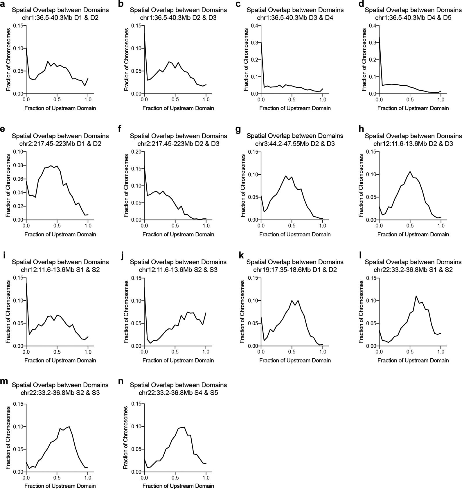
a, Distribution of spatial overlap between neighboring domains (D1 & D2) at chr1:36.5–40.3Mb. Overlap normalized to the volume of the upstream domain. n = 2294 chromosomes. b, Distribution of spatial overlap between neighboring domains (D2 & D3) at chr1:36.5–40.3Mb. Overlap normalized to the volume of the upstream domain. n = 2553 chromosomes. c, Distribution of spatial overlap between neighboring domains (D3 & D4) at chr1:36.5–40.3Mb. Overlap normalized to the volume of the upstream domain. n = 2502 chromosomes. d, Distribution of spatial overlap between neighboring domains (D4 & D5) at chr1:36.5–40.3Mb. Overlap normalized to the volume of the upstream domain. n = 9443 chromosomes. e, Distribution of spatial overlap between neighboring domains (D1 & D2) at chr2:217.45–223Mb. Overlap normalized to the volume of the upstream domain. n = 1850 chromosomes. f, Distribution of spatial overlap between neighboring domains (D2 & D3) at chr2:217.45–223Mb. Overlap normalized to the volume of the upstream domain. n = 1903 chromosomes. g, Distribution of spatial overlap between neighboring domains (D2 & D3) at chr3:44.2–47.55Mb. Overlap normalized to the volume of the upstream domain. n = 1657 chromosomes. h, Distribution of spatial overlap between neighboring domains (D2 & D3) at chr12:11.6–13.6Mb. Overlap normalized to the volume of the upstream domain. n = 1606 chromosomes. i, Distribution of spatial overlap between neighboring domains (S1 & S2) at chr12:11.6–13.6Mb. Overlap normalized to the volume of the upstream domain. n = 1479 chromosomes. j, Distribution of spatial overlap between neighboring domains (S2 & S3) at chr12:11.6–13.6Mb. Overlap normalized to the volume of the upstream domain. n = 1912 chromosomes. k, Distribution of spatial overlap between neighboring domains (D1 & D2) at chr19:17.35–18.6Mb. Overlap normalized to the volume of the upstream domain. n = 1406 chromosomes. l, Distribution of spatial overlap between neighboring domains (S1 & S2) at chr22:33.2–36.8Mb. Overlap normalized to the volume of the upstream domain. n = 1634 chromosomes. m, Distribution of spatial overlap between neighboring domains (S2 & S3) at chr22:33.2–36.8Mb. Overlap normalized to the volume of the upstream domain. n = 1640 chromosomes. n, Distribution of spatial overlap between neighboring domains (S4 & S5) at chr22:33.2–36.8Mb. Overlap normalized to the volume of the upstream domain. n = 1494 chromosomes.

Extended Data Fig. 4. Additional information related to Figure 2.

a, Localization density per domain quantified from 3D-STORM images. Chr12.D1 (median = 0.0002707, n = 91); Chr12.D2 (median = 0.0002076, n = 91); Chr22.D1 (median = 0.0002376, n = 95); Chr22.D2 (median = 0.0002245, n = 95). b, Scatterplot depicting the relationship between domain volumes on the same chromosome by 3D-STORM on chr12:11.6Mb-13.6Mb. n = 91 chromosomes. c, Scatterplot depicting the relationship between domain volumes between homologs by 3D-STORM on chr12:11.6Mb-13.6Mb. n = 82 chromosomes. d, Scatterplot depicting the relationship between domain volumes on the same chromosome by 3D-STORM on chr22:33.2Mb-36.8Mb. n = 95 chromosomes. e, Scatterplot depicting the relationship between domain volumes between homologs by 3D-STORM on chr22:33.2Mb-36.8Mb. n = 86 chromosomes. f, Scatterplot of overlap volume (x-axis) versus domain density (y-axis) by 3D-STORM for the chr22:33.2Mb-36.8Mb locus. n = 95 chromosomes.

Extended Data Fig. 5. Confirmation and quantification of RAD21 degradation.

a, Immunofluorescence for RAD21 (cyan). DNA (Hoescht stain) is shown in grey. Dashed lines represent nuclear edges. Scale bar equals 5 μm. b, Western blot to RAD21 protein in the chromatin-bound fraction of HCT-116-RAD21-AID cells with no auxin treatment (−) or following 6 hours of auxin treatment (+). Histone H3 as loading control. Protein was labeled using fluorescent secondary antibodies. c, Fluorescence quantification of RAD21 and H3 isolated from the chromatin-bound fraction of protein corresponding to blot in b using Image Lab v5.2.1. Protein intensity normalized to total protein per well (via stain-free technology) and presented as fraction of protein observed in untreated (− auxin) conditions; we observe a 96% reduction in chromatin-bound RAD21 following auxin treatment.

Extended Data Fig. 6. Cohesin promotes interactions across domain boundaries (additional loci).

Hi-C contact matrix and corresponding cumulative distribution of spatial overlap between the neighboring domains prior to or after auxin treatment. Overlap normalized to the volume of the upstream domain. a, Map of chr1:36.5–40.3Mb for b-e. b, D1 & D2 (−aux n = 2294, +aux n = 2175). c, D2 & D3 (−aux n = 2553, +aux n = 2353). d, D3 & D4 (−aux n = 2502, +aux n = 2488), e. D4 & D5 (−aux n = 9443, +aux n = 8695). f, Map of chr2:217.45–223Mb for g-h. g, D1 & D2 (−aux n = 1850, +aux n = 1665). h, D2 & D3 (−aux n = 1903, +aux n = 1717). i, Map of chr3:44.2–47.55Mb for j-k. j, D1 & D2 (−aux n = 1643, +aux n = 2186). k, D2 & D3 (−aux n = 1657, +aux n = 2181). l, Map of chr12:11.6–13.6Mb for m-o. m, D2 & D3 (−aux n = 1606, +aux n = 1570). n, S1 & S2 (−aux n = 1479, +aux n = 1220). o, S2 & S3 (−aux n = 731, +aux n = 678). p, Map of chr19:17.35–18.6Mb for q. q, D1 & D2 (−aux n = 1406, +aux n = 1419). r, Map of chr22:33.2–36.8Mb for s-u. s, S1 & S2 (−aux n = 1634, +aux n = 1703). t, S2 & S3 (−aux n = 1640, +aux n = 1702). u, S4 & S5 (−aux n = 1494, +aux n = 1718). P < 0.001, two-tailed Mann-Whitney test for all domain pairs.

Extended Data Fig. 7. Additional information related to Figure 3.

a, Minimum distances between localizations contained within each domain on chr12:11.6–13.6Mb as measured from 3D-STORM data (prior to auxin: median = 0.008292 μm, n = 91; after auxin: median = 0.01234 μm, n = 76). P < 0.001, two-tailed Mann-Whitney test. b, Minimum distances between localizations contained within each domain on chr22:33.2Mb-36.8Mb as measured from 3D-STORM data (prior to auxin: median = 0.009470 μm, n = 95; after auxin: median = 0.01563 μm, n = 105). P < 0.001, two-tailed Mann-Whitney test. c, Violin plots of domain volumes as measured from 3D-STORM data prior to [Chr12.D1 (median = 0.2629 μm³, n = 91); Chr12.D2 (median = 0.1830 μm³, n = 91); Chr22.D1 (median = 0.2749 μm³, n = 95); Chr22.D2 (median = 0.2320 μm³, n = 95)] or after auxin treatment [Chr12.D1 (median = 0.1703 μm³, n = 91); Chr12.D2 (median = 0.1671 μm³, n = 76); Chr22.D1 (median = 0.2284 μm³, n = 105); Chr22.D2 (median = 0.2213μm³, n = 105)]. Chr12.D1 P = 0.008; Chr12.D2 P = 0.368; Chr22.D1 P = 0.076, Chr22.D2 P = 0.907; two-tailed Mann-Whitney test. d, Violin plots of domain densities as measured from 3D-STORM data prior to [Chr12.D1 (median = 0.0002707, n = 91); Chr12.D2 (median = 0.0002076, n = 91); Chr22.D1 (median = 0.0002376, n = 95); Chr22.D2 (median = 0.0002245, n = 95)] or after auxin treatment [Chr12.D1 (median = 0.0003080, n = 76); Chr12.D2 (median = 0.0002385, n = 76); Chr22.D1 (median = 0.0002651, n = 105); Chr22.D2 (median = 0.0002353, n = 105)]. Chr12.D1 P = 0.247; Chr12.D2 P = 0.014; Chr22.D1 P = 0.025, Chr22.D2 P = 0.602; two-tailed Mann-Whitney test.

Extended Data Fig. 8. Additional information related to Figure 4.

a, Western blot of NIPBL, WAPL, and CTCF protein of HCT-116 cells following RNAi. H3 as loading control. b, Representative FISH images of neighboring domains on chr12:11.6Mb-13.6Mb in RNAi control, NIPBL-, WAPL-, or CTCF-depleted cells. Dashed lines represent nuclear edges. Scale bar equals 5 μm (left) or 1 μm (zoomed images, below). c, Spatial overlap between neighboring domains on chr12:11.6Mb-13.6Mb in control (n = 643), NIPBL- (n = 636), WAPL- (n = 819) or both NIPBL and WAPL- (n = 922) depleted cells. ***P < 0.001, two-tailed Mann-Whitney test. d, Spatial overlap between neighboring domains on chr22:33.2Mb-36.8Mb in control (n = 1722), NIPBL- (n = 1440), WAPL- (n = 1769) or both NIPBL and WAPL- (n = 1762) depleted cells. Overlap normalized to the volume of the upstream domain. ***P < 0.001, two-tailed Mann-Whitney test. e, Western blot to RAD21 and CTCF in whole cell lysate of HCT-116 cells following RNAi to CTCF and/or 6 hours auxin to degrade RAD21. Alpha tubulin as loading control. Spatial overlap between neighboring domains across six loci (f-k). f, D4 and D5 on chr1:36.5–40.3Mb in control (n = 2362) or CTCF- (n = 1611) depleted cells. ***P < 0.001. two-tailed Mann-Whitney test. g, D1 and D2 on chr2:217.45–223Mb in control (n = 1484) or CTCF- (n = 1466) depleted cells. P = 0.604 (ns). two-tailed Mann-Whitney test. h, D2 and D3 on chr2:217.45–223Mb in control or CTCF-depleted cells prior to (control n = 1145; CTCF n = 1133) or after auxin treatment (control n = 1039; CTCF n = 877). P < 0.001 (***), P = 0.008 (**). two-tailed Mann-Whitney test. i, D1 and D2 on chr3:44.2–47.55Mb in control or CTCF-depleted cells prior to (control n = 1272; CTCF n = 1215) or after auxin treatment (control n = 1254; CTCF n = 1090). P < 0.001 (***) or P = 0.996. two-tailed Mann-Whitney test. j, D1 and D2 on chr12:11.6Mb-13.6Mb in control or CTCF-depleted cells prior to (control n = 1236; CTCF n = 1250) or after auxin treatment (control n = 1174; CTCF n = 1231). P < 0.001 (***) or P = 0.314. two-tailed Mann-Whitney test. k, D1 and D2 on chr22:33.2–36.8Mb in control or CTCF-depleted cells prior to (control n = 1258; CTCF n = 1370) or after auxin treatment (control n = 1170; CTCF n = 1157). P < 0.001 (***) or P = 0.89, two-tailed Mann-Whitney test.

Extended Data Fig. 9. Additional information related to Figure 5.

a, Hi-C contact matrix chr12:11.6–13.6Mb and corresponding Oligopaint design for (b-c). Blue represents the boundary proximal gene, CREBL2. b, Cartoon representations for three possible interactions between boundary-proximal genes and their neighboring domains: domain maintenance, switching, and exclusion (top). Representative images of three-color FISH to the chr12:11.6–13.6Mb locus illustrating the three domain configurations (middle); scale bar equals 1 μm. Corresponding 3D segmentation of FISH signals below each image. c, Frequencies of domain configurations at chr12:11.6–13.6Mb prior to (n = 1074) or after auxin treatment (n = 979). P < 0.0001 (***) or P = 0.0046 (**), two-sided Fisher’s exact test.

Extended Data Fig. 10. Additional information related to Figure 6.

a, Distribution of domain sizes that harbor either a significantly differentially expressed (median = 183734, n = 4196) or non-differentially expressed genes (median = 194447, n = 8026) in the HCT-116 cell line following auxin treatment. P = 0.102, two-tailed Mann-Whitney test. b, Scatterplot of log₂(fold change)] of HCT-116 differentially expressed genes (DEGs) versus the distance between their TSS and the center of the nearest domain boundary. c, Distance to nearest super enhancer defined by H3K27ac signal⁵⁸ in HCT-116 cells for DEGs with >30% fold change in expression following auxin treatment. Genes were categorized by their proximity to a domain boundary (< 5kb or > 5kb away) and whether they were up or down regulated following auxin treatment. d, Gene ontology enrichment analysis for HCT-116 differentially expressed genes (> 30% fold change, n = 68) within 5kb of a domain boundary. e, Gene ontology enrichment analysis for HCT-116 differentially expressed genes (> 30% fold change, n = 1593) not within 5kb of a domain boundary. f, Scatterplot of [fold change] of differentially expressed genes (DEGs) associated with CdLS versus the distance between their TSS and the center of the nearest domain boundary in GM12878 cells. n = 1569, P = 0.0017, Spearman correlation. g, Fraction of genes that are up or down regulated in CdLS at binned distances from the nearest domain boundary. h, Fold change in burst volume by RNA FISH in HCT-116 cells following auxin treatment. Each dot represents the fold change in average burst volume per biological replicate; horizonal line indicates mean.

References

- 1.Bickmore WA The spatial organization of the human genome. Annu Rev Genomics Hum Genet 14, 67–84 (2013). [DOI] [PubMed] [Google Scholar]
- 2.Gibcus JH & Dekker J The hierarchy of the 3D genome. Mol Cell 49, 773–82 (2013). [DOI] [PMC free article] [PubMed] [Google Scholar]
- 3.Cremer T & Cremer M Chromosome territories. Cold Spring Harbor perspectives in biology 2, a003889 (2010). [DOI] [PMC free article] [PubMed] [Google Scholar]
- 4.Hansen AS, Pustova I, Cattoglio C, Tjian R & Darzacq X CTCF and cohesin regulate chromatin loop stability with distinct dynamics. Elife 6(2017). [DOI] [PMC free article] [PubMed] [Google Scholar]
- 5.Kim YH et al. Rev-erbalpha dynamically modulates chromatin looping to control circadian gene transcription. Science 359, 1274–1277 (2018). [DOI] [PMC free article] [PubMed] [Google Scholar]
- 6.Phillips-Cremins JE et al. Architectural protein subclasses shape 3D organization of genomes during lineage commitment. Cell 153, 1281–95 (2013). [DOI] [PMC free article] [PubMed] [Google Scholar]
- 7.Rao SS et al. A 3D map of the human genome at kilobase resolution reveals principles of chromatin looping. Cell 159, 1665–80 (2014). [DOI] [PMC free article] [PubMed] [Google Scholar]
- 8.Rao SSP et al. Cohesin Loss Eliminates All Loop Domains. Cell 171, 305–320 e24 (2017). [DOI] [PMC free article] [PubMed] [Google Scholar]
- 9.Dixon JR et al. Topological domains in mammalian genomes identified by analysis of chromatin interactions. Nature 485, 376–80 (2012). [DOI] [PMC free article] [PubMed] [Google Scholar]
- 10.Nora EP et al. Spatial partitioning of the regulatory landscape of the X-inactivation centre. Nature 485, 381–5 (2012). [DOI] [PMC free article] [PubMed] [Google Scholar]
- 11.Zhan Y et al. Reciprocal insulation analysis of Hi-C data shows that TADs represent a functionally but not structurally privileged scale in the hierarchical folding of chromosomes. Genome Res 27, 479–490 (2017). [DOI] [PMC free article] [PubMed] [Google Scholar]
- 12.Sexton T et al. Three-dimensional folding and functional organization principles of the Drosophila genome. Cell 148, 458–72 (2012). [DOI] [PubMed] [Google Scholar]
- 13.Le Dily F et al. Distinct structural transitions of chromatin topological domains correlate with coordinated hormone-induced gene regulation. Genes Dev 28, 2151–62 (2014). [DOI] [PMC free article] [PubMed] [Google Scholar]
- 14.Sun F et al. Promoter-Enhancer Communication Occurs Primarily within Insulated Neighborhoods. Mol Cell 73, 250–263 e5 (2019). [DOI] [PMC free article] [PubMed] [Google Scholar]
- 15.Dowen JM et al. Control of cell identity genes occurs in insulated neighborhoods in mammalian chromosomes. Cell 159, 374–387 (2014). [DOI] [PMC free article] [PubMed] [Google Scholar]
- 16.Lupianez DG et al. Disruptions of topological chromatin domains cause pathogenic rewiring of gene-enhancer interactions. Cell 161, 1012–1025 (2015). [DOI] [PMC free article] [PubMed] [Google Scholar]
- 17.Sanborn AL et al. Chromatin extrusion explains key features of loop and domain formation in wild-type and engineered genomes. Proc Natl Acad Sci U S A 112, E6456–65 (2015). [DOI] [PMC free article] [PubMed] [Google Scholar]
- 18.Goloborodko A, Marko JF & Mirny LA Chromosome Compaction by Active Loop Extrusion. Biophys J 110, 2162–8 (2016). [DOI] [PMC free article] [PubMed] [Google Scholar]
- 19.Mirny LA, Imakaev M & Abdennur N Two major mechanisms of chromosome organization. Curr Opin Cell Biol 58, 142–152 (2019). [DOI] [PMC free article] [PubMed] [Google Scholar]
- 20.Wendt KS et al. Cohesin mediates transcriptional insulation by CCCTC-binding factor. Nature 451, 796–801 (2008). [DOI] [PubMed] [Google Scholar]
- 21.Splinter E et al. CTCF mediates long-range chromatin looping and local histone modification in the beta-globin locus. Genes Dev 20, 2349–54 (2006). [DOI] [PMC free article] [PubMed] [Google Scholar]
- 22.Lieberman-Aiden E et al. Comprehensive mapping of long-range interactions reveals folding principles of the human genome. Science 326, 289–93 (2009). [DOI] [PMC free article] [PubMed] [Google Scholar]
- 23.Nora EP et al. Targeted Degradation of CTCF Decouples Local Insulation of Chromosome Domains from Genomic Compartmentalization. Cell 169, 930–944 e22 (2017). [DOI] [PMC free article] [PubMed] [Google Scholar]
- 24.Schwarzer W et al. Two independent modes of chromatin organization revealed by cohesin removal. Nature 551, 51–56 (2017). [DOI] [PMC free article] [PubMed] [Google Scholar]
- 25.Wutz G et al. Topologically associating domains and chromatin loops depend on cohesin and are regulated by CTCF, WAPL, and PDS5 proteins. EMBO J 36, 3573–3599 (2017). [DOI] [PMC free article] [PubMed] [Google Scholar]
- 26.Nagano T et al. Single-cell Hi-C reveals cell-to-cell variability in chromosome structure. Nature 502, 59–64 (2013). [DOI] [PMC free article] [PubMed] [Google Scholar]
- 27.Bintu B et al. Super-resolution chromatin tracing reveals domains and cooperative interactions in single cells. Science 362(2018). [DOI] [PMC free article] [PubMed] [Google Scholar]
- 28.Finn EH et al. Extensive Heterogeneity and Intrinsic Variation in Spatial Genome Organization. Cell 176, 1502–1515 e10 (2019). [DOI] [PMC free article] [PubMed] [Google Scholar]
- 29.Flyamer IM et al. Single-nucleus Hi-C reveals unique chromatin reorganization at oocyte-to-zygote transition. Nature 544, 110–114 (2017). [DOI] [PMC free article] [PubMed] [Google Scholar]
- 30.Beliveau BJ et al. Single-molecule super-resolution imaging of chromosomes and in situ haplotype visualization using Oligopaint FISH probes. Nat Commun 6, 7147 (2015). [DOI] [PMC free article] [PubMed] [Google Scholar]
- 31.Beliveau BJ et al. Versatile design and synthesis platform for visualizing genomes with Oligopaint FISH probes. Proc Natl Acad Sci U S A 109, 21301–6 (2012). [DOI] [PMC free article] [PubMed] [Google Scholar]
- 32.Beliveau BJ et al. OligoMiner provides a rapid, flexible environment for the design of genome-scale oligonucleotide in situ hybridization probes. Proc Natl Acad Sci U S A 115, E2183–E2192 (2018). [DOI] [PMC free article] [PubMed] [Google Scholar]
- 33.Beliveau BJ, Apostolopoulos N & Wu CT Visualizing genomes with Oligopaint FISH probes. Curr Protoc Mol Biol 105, Unit 14 23 (2014). [DOI] [PMC free article] [PubMed] [Google Scholar]
- 34.Beliveau BJ et al. In Situ Super-Resolution Imaging of Genomic DNA with OligoSTORM and OligoDNA-PAINT. Methods Mol Biol 1663, 231–252 (2017). [DOI] [PMC free article] [PubMed] [Google Scholar]
- 35.Shin H et al. TopDom: an efficient and deterministic method for identifying topological domains in genomes. Nucleic Acids Res 44, e70 (2016). [DOI] [PMC free article] [PubMed] [Google Scholar]
- 36.Consortium EP An integrated encyclopedia of DNA elements in the human genome. Nature 489, 57–74 (2012). [DOI] [PMC free article] [PubMed] [Google Scholar]
- 37.Ollion J, Cochennec J, Loll F, Escude C & Boudier T TANGO: a generic tool for high-throughput 3D image analysis for studying nuclear organization. Bioinformatics 29, 1840–1 (2013). [DOI] [PMC free article] [PubMed] [Google Scholar]
- 38.Chang LH, Ghosh S & Noordermeer D TADs and Their Borders: Free Movement or Building a Wall? J Mol Biol (2019). [DOI] [PubMed] [Google Scholar]
- 39.Natsume T, Kiyomitsu T, Saga Y & Kanemaki MT Rapid Protein Depletion in Human Cells by Auxin-Inducible Degron Tagging with Short Homology Donors. Cell Rep 15, 210–218 (2016). [DOI] [PubMed] [Google Scholar]
- 40.Nasmyth K & Haering CH Cohesin: its roles and mechanisms. Annu Rev Genet 43, 525–58 (2009). [DOI] [PubMed] [Google Scholar]
- 41.Eisenberg E & Levanon EY Human housekeeping genes, revisited. Trends Genet 29, 569–74 (2013). [DOI] [PubMed] [Google Scholar]
- 42.Dorsett D & Krantz ID On the molecular etiology of Cornelia de Lange syndrome. Ann N Y Acad Sci 1151, 22–37 (2009). [DOI] [PMC free article] [PubMed] [Google Scholar]
- 43.Liu J et al. Transcriptional dysregulation in NIPBL and cohesin mutant human cells. PLoS Biol 7, e1000119 (2009). [DOI] [PMC free article] [PubMed] [Google Scholar]
- 44.Nir G et al. Walking along chromosomes with super-resolution imaging, contact maps, and integrative modeling. PLoS Genet 14, e1007872 (2018). [DOI] [PMC free article] [PubMed] [Google Scholar]
- 45.Cardozo Gizzi AM et al. Microscopy-Based Chromosome Conformation Capture Enables Simultaneous Visualization of Genome Organization and Transcription in Intact Organisms. Mol Cell 74, 212–222 e5 (2019). [DOI] [PubMed] [Google Scholar]
- 46.Nuebler J, Fudenberg G, Imakaev M, Abdennur N & Mirny LA Chromatin organization by an interplay of loop extrusion and compartmental segregation. Proc Natl Acad Sci U S A 115, E6697–E6706 (2018). [DOI] [PMC free article] [PubMed] [Google Scholar]
- 47.Haarhuis JHI et al. The Cohesin Release Factor WAPL Restricts Chromatin Loop Extension. Cell 169, 693–707 e14 (2017). [DOI] [PMC free article] [PubMed] [Google Scholar]
- 48.Thiecke MJ et al. Cohesin-dependent and independent mechanisms support chromosomal contacts between promoters and enhancers. bioRxiv (2020). [DOI] [PMC free article] [PubMed] [Google Scholar]
- 49.Bartman CR, Hsu SC, Hsiung CC, Raj A & Blobel GA Enhancer Regulation of Transcriptional Bursting Parameters Revealed by Forced Chromatin Looping. Mol Cell 62, 237–247 (2016). [DOI] [PMC free article] [PubMed] [Google Scholar]
- 50.Durand NC et al. Juicer Provides a One-Click System for Analyzing Loop-Resolution Hi-C Experiments. Cell Syst 3, 95–8 (2016). [DOI] [PMC free article] [PubMed] [Google Scholar]
- 51.Moffitt JR & Zhuang X RNA Imaging with Multiplexed Error-Robust Fluorescence In Situ Hybridization (MERFISH). Methods Enzymol 572, 1–49 (2016). [DOI] [PMC free article] [PubMed] [Google Scholar]
- 52.Rosin LF, Nguyen SC & Joyce EF Condensin II drives large-scale folding and spatial partitioning of interphase chromosomes in Drosophila nuclei. PLoS Genet 14, e1007393 (2018). [DOI] [PMC free article] [PubMed] [Google Scholar]
- 53.Ollion J, Cochennec J, Loll F, Escude C & Boudier T Analysis of nuclear organization with TANGO, software for high-throughput quantitative analysis of 3D fluorescence microscopy images. Methods Mol Biol 1228, 203–22 (2015). [DOI] [PubMed] [Google Scholar]
- 54.Kishi JY et al. SABER amplifies FISH: enhanced multiplexed imaging of RNA and DNA in cells and tissues. Nat Methods 16, 533–544 (2019). [DOI] [PMC free article] [PubMed] [Google Scholar]
- 55.Liao Y, Wang J, Jaehnig EJ, Shi Z & Zhang B WebGestalt 2019: gene set analysis toolkit with revamped UIs and APIs. Nucleic Acids Res 47, W199–W205 (2019). [DOI] [PMC free article] [PubMed] [Google Scholar]
- 56.Durand NC et al. Juicebox provides a visualization system for Hi-C contact maps with unlimited zoom. Cell Syst. 3, 99–101 (2016). [DOI] [PMC free article] [PubMed] [Google Scholar]
- 57.Robinson JT et al. Integrative genomics viewer. _Nat. Biotechnol_29, 24–26 (2011). [DOI] [PMC free article] [PubMed] [Google Scholar]
- 58.Hnisz D, Day DS & Young RA Insulated neighborhoods: structural and functional units of mammalian gene control._Cell_167, 1188–1200 (2016). [DOI] [PMC free article] [PubMed] [Google Scholar]
Associated Data
This section collects any data citations, data availability statements, or supplementary materials included in this article.