sMRT: Multi-Resident Tracking in Smart Homes with Sensor Vectorization

Abstract

Smart homes equipped with anonymous binary sensors offer a low-cost, unobtrusive solution that powers activity-aware applications such as building automation, health monitoring, behavioral intervention and home security. However, when there are multiple residents living in the smart home, the data association between sensor events and residents can pose a major challenge. Previous approaches to multi-resident tracking in smart homes rely on extra information, such as sensor layout, floor plan and annotated data, which may not be available or inconvenient to obtain in practice. To address those challenges in real-life deployment, we introduce the sMRT algorithm that simultaneously tracks the location of each resident and estimates the number of residents in the smart home, without relying on ground-truth annotated sensor data or other additional information. We evaluate the performance of our approach using two smart home datasets recorded in real-life settings and compare sMRT with two other methods that rely on sensor layout and ground truth-labeled sensor data.

1. Introduction

SMART homes offer a promising technology that combines sensor networks and artificial intelligence algorithms to improve the living experience and productivity of residents. With the ability to comprehend and predict the daily activities of residents, smart homes can offer context-aware services such as home automation and health monitoring. Home automation services can reduce energy consumption and improve living comfort for residents by anticipating their behavior inside the smart home. In the case of health monitoring, smart homes are capable of detecting behavior patterns that indicate sudden or gradual changes in cognitive, mobility, and physical health states. Because a majority of existing smart home research is limited to single-resident environments, there remains a challenge of how to extend this work to encompass multi-resident scenarios.

In this paper, we introduce a method to tackle the multi-resident tracking problem in smart homes. This includes both estimating the number of active residents in the environment as well as associating sensor data with residents. One of the major challenges in multi-resident scenarios is associating sensor data with the corresponding individuals who caused the change in state. One solution to this data association problem, and to resident tracking in general, is attaching tracking devices, including mobile phones or smart watches, to smart home residents. In these cases, the residents are responsible for correctly wearing the devices at all times and they cannot share their devices with other residents. Those additional constraints on the residents are usually inconvenient in practice and not reliable in real-life deployment. Moreover, such user-specific sensor devices are tailored toward monitoring one persons movements rather than all of the activities that occur within the space, which represents valuable information for recognition and analysis of daily activities. Surveillance cameras, on the other hand, offer rich information that can be used to recognize the resident in the video as well as infer the activity that is being performed. Multiple data fusion and tracking algorithms have been proposed in the literature to identify and track each resident in multiple video streams [1], [2], [3], [4]. However, in addition to facing challenges with lighting and obstruction, cameras are often considered too intrusive to be used in homes due to privacy concerns.

Ambient sensors, which include motion sensors, door sensors, temperature/light sensors, and contact-based item sensors, offer a low-cost and less-intrusive solution for smart home applications. As the data collected by these sensors are not associated with any specific resident, the data association problem presents a major challenge when multiple people are present in the smart home at the same time. Association can be simplified by assuming that the number of residents in the space is constant. Another simplification is to take advantage of additional information that may be available, such as the floor plan of the smart home and the position of sensors in the space. However, in reality, the number of residents in the smart home may change when neighbors, friends or family members come to visit and information about floor plans and sensor layouts may be impractical to obtain in real-life deployments. In contrast to prior approaches, our proposed multi-resident analysis strategy focuses on tracking residents and associating the residents with the sensor data they trigger in the smart home without additional information such as the floorplan or sensor layout, while at the same time estimating the number of residents that currently inhabit the smart home.

Here we introduce sMRT, an algorithm that performs multi-resident tracking in smart environments. Instead of requiring a floorplan and sensor map, sMRT learns the spatiotemporal relationship between ambient sensors from available unlabeled sensor data. Based on the learned relationships, sMRT then applies a multi-target Gaussian mixture probability hypothesis density (GM-PHD) filter to estimate the number of residents that are currently present in the smart home, track their locations, and associate each of them with triggered sensor events.

To validate the approach, we evaluate sMRT using data collected from actual smart homes with ground truth-labeled resident data associations. We compare the performance of sMRT with both a local nearest neighbor tracker and a global nearest neighbor tracker, both of which utilize a hand-crafted actual sensor layout of the smart home. We evaluate performance both for tracking accuracy and accuracy of estimating the number of residents present in the smart home at any given time. The result shows that the sMRT algorithm achieves a comparable accuracy than alternative approaches. Additionally, sMRT offers the ability to concurrently estimate the number of residents.

2. Related Work

Passive ambient sensors offer an unobtrusive technology for monitoring the daily routine of smart home residents. Past research has shown that these sensors provide the information needed for activity recognition [5], [6], [7], [8], [9], activity forecasting [10], [11], [12], and activity-aware applications. Example activity-aware applications include health monitoring [13], [14], [15], [16], [17], [18], [19], behavior intervention [20], home security [21], [22], [23], and building automation [24], [25], [26], [27], [28]. However, in a multi-resident scenario, the sensor events recorded in a smart home need to be segregated into multiple tracks before being consumed by the activity-aware applications. Each track is composed of a series of sensor events corresponding to one of the residents inhabiting the smart home.

Past related research has built a foundation for multi-resident tracking in smart homes. The multi-resident tracking problem is usually formulated as a data association problem between sensor events and the residents inhabiting the smart home. The tracking approaches proposed in the literature vary depending on the assumptions of information availability. Some work assumes that the floor plan and location of sensors deployed in the smart homes are readily available. Other work assumes that the activity and motion model of each resident or all residents in the smart home can be constructed using annotated data or through controlled experiments. The multi-resident tracking problem can be greatly simplified if the number of residents in the smart home is known a priori. In this section, we provide a discussion of each of these research directions.

Both Wilson et. al. [29] and Hsu et. al. [30] focus on the design and training of a behavioral model to solve the resident tracking and activity recognition problems simultaneously in a smart home inhabited with multiple residents. In both works, the number of residents in the smart home is specified a priori and remains constant. Provided annotated data, Wilson et. al. [29] train a hidden Markov model (HMM) in which the hidden states represent both the activity and the location of all residents while the observable states map to all the sensors deployed in the smart home. The data association problem is thus equivalent to the HMM inference problem and is solved using a Rao-Backwellised particle filter (RBPF). Similarly, based on annotated data Hsu et. al. [30] train three conditional random fields (CRF) to model the relationship between activities, residents, and sensor events. The data association problem is solved using an iterative inference algorithm.

Crandall and Cook [31], [32], on the other hand, formulate the problem of associating sensor events with the residents in smart home as a multi-class classification problem. Given annotated data and a fixed number of residents to track, a naïve Bayes classifier and a Markov model classifier are trained to predict the associated resident with a series of sensor events as the input. Their work concludes that there are subtle differences between multiple people performing the same activity in the same environment and such differences can be detected using machine learning algorithms.

Other work focuses on estimating the transition probabilities between sensors deployed in the smart home. This represents a valuable pre-processing step for multi-resident tracking. The graph model that encodes the transition probabilities, also referred to as a Bayes updating graph [33], sensor graph [34], or accessibility graph [35], is equivalent to a Markov chain where states are mapped directly to all the sensors deployed in the smart home. The structure and parameters of the model are derived based on the smart home sensor layout as well as annotated sensor data. The models are used in combination with a rule-based tracker [33] and a multi-hypothesis tracker [34] to solve the data association problem. These multi-resident tracking solutions also have the ability to estimate the number of residents in the smart home, although they rely on the availability of a hand-crafted sensor graph that is based on known locations of sensors in the floorplan as well as annotated data to derive transition probabilities.

Provided with the sensor layout and the floorplan of the smart home, Amri et. al. [36] and Song and Wang [37] solve the data association problem by modeling the sensor coverage as well as the spatial relationships between deployed sensors in the smart home. Amri et. al. [36] overlay a square box on the floorplan to model the coverage of motion sensors, and formulate the motion sensor-based multi-resident tracking problem within a set-membership estimation framework. Song and Wang [37] introduce a unit disk graph to represent the field of focus of all sensors and propose a multi-color particle filter to associate sensor events with the residents.

De et. al. [38] and Wang et. al. [39] propose the idea of mining possible motion trajectories of smart home residents directly from the recorded sensor events. Various data association hypotheses are created by fitting the mined trajectories to the incoming sensor events. The best hypothesis is chosen so that the average velocity variance among all residents is minimized. In order to calculate the average velocity variance, the adjacency and distance between sensors are considered as available information. The algorithm performs better if the number of residents is known during the trajectory mining phase.

3. Smart Home Datasets and Multi-Resident Tracking in Smart Homes

The multi-resident tracking algorithm proposed in this work analyzes sensor events recorded in smart homes equipped with passive ambient sensors. These ambient sensors generate information about the location of the residents in the smart home or the interaction between the residents and the objects of interest in the home. The states of the sensors are usually binary, as they are either “active” or “inactive” at any given moment. The state transition of these sensors is usually triggered by resident activity. A sensor will send an “activate” message when the state transitions from “inactive” to “active”, followed by a “deactive” message when the state transitions to “inactive” again. However, these sensors are all anonymous, as they lack the ability to directly identify the resident that triggers the messages. As a result, a tracking algorithm is needed to pair sensor messages with the associated residents in a smart home occupied by multiple residents.

We introduce sMRT, an algorithm to automate multi-resident tracking in smart environments. To illustrate our methods and evaluate the approach implemented in sMRT, we utilize two multi-resident smart home datasets created by the Center of Advanced Studies in Adaptive Systems (CASAS) at Washington State University. The floor plan and the layout of deployed sensors for these two smart home datasets are shown in Figure 1. The dataset named TM004¹ (in Figure 1a) contains December 2016 data recorded in a two-bedroom apartment with two older adult residents monitored by 25 ambient sensors distributed among 8 rooms. Occasionally, their child will come and stay in their house for a couple of days. The site is coarsely monitored with an average of 2–3 PIR motion sensors per room. Residents can enter the house from the garage on the bottom left, from the back yard through the door on the right, and through the main entrance located at the bottom middle.

Fig. 1.

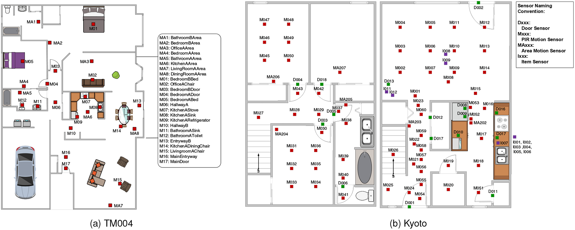
Floor plan and the locations of sensors deployed in CASAS smart homes. (a) Smart home TM004 with 25 motion sensors. (b) Smart home site Kyoto with 65 motion sensors, 15 door sensors and 11 item sensors.

Figure 1b shows a second smart home named Kyoto, a two-story town house¹. Compared with TM004, Kyoto contains a denser grid of sensors. Both scripted and unscripted data has been collected in Kyoto and is associated with a number of studies including earlier approaches to multi-resident tracking [31]. We analyze data collected in 2009 while two residents lived in the apartment and performed their normal, unscripted daily routines. Occasionally, friends would visit for a few days, increasing the number of residents in the home. Data are collected from 91 sensors installed in 6 rooms: bedrooms, bathroom, kitchen, dining room, and living room as well as along hallways. Additionally, magnetic door sensors are positioned on front and back exterior doors as well as cabinets, closets and refrigerator doors. A few items of interest are equipped with contact sensors where the information about resident interaction with these items can provide insights into the activity they are performing at the time. Due to limitations of this earlier smart home technology, an increased number of false-positive sensor events and out-of-order sensor event sequences occur in Kyoto as compared with TM004. This issue has been documented in prior work [33].

In both datasets, local PIR motion sensors (sensors with a 1 meter diameter) and area motion sensors (sensors that monitor an entire room or large area) send an “ON” message when resident motion is detected within the sensor’s field of view (“active” state), and an “OFF” message when the motion is no longer detected (“inactive” state). The magnetic door sensor sends an “OPEN” message when the door is opened (“active” state) and a “CLOSE” message when the door is closed (“inactive” state). Contact-based item sensors produce an “ABSENT” message when the item is removed from the sensor (“active” state) and a “PRESENT” message when the item is put back into place (“inactive” state). Messages are sent to the smart home server which tags them with the time when the messages are received. Throughout this paper, we use sensor event to refer to the subset of sensor messages that contain an “active state” (or “activate”) message. We do not include the corresponding “inactive state” (or “deactivate”) messages as sensor events. The goal of multi-resident tracking is to associate each sensor event with the resident who activates the sensor.

Table 1 shows a series of sensor messages recorded at Kyoto. Each sensor message is a 3-tuple consisting of the message timestamp, the sensor ID, and the message content. To provide ground-truth information for evaluating multi-resident tracking solutions, external annotators label each sensor event with an identifier for the resident(s) who triggers the sensor message, as shown in the “Residents” column. Annotators generate labels based on information from raw sensor data and a visualization of sensor observations superimposed on the smart home floorplan, provided by the ActViz tool². External annotators prevent interrupting resident reports to self-report such labels. This process also improves label consistency. As shown in Figure 2, ActViz maps each sensor event to the smart home floorplan. Thus, human annotators can examine the motion of each resident alongside their previous behavior when annotating each sensor message with the associated resident identifiers and associated activity labels. The TM004 dataset used in our evaluation contains 9 days of annotated data containing 98,506 sensor events. The Kyoto dataset contains 3 days of annotated data containing 28,923 sensor events.

TABLE 1.

An example of sensor messages recorded in the Kyoto dataset. Each sensor message is a three-tuple consisting of the timestamp, sensor ID and message content. The resident and activity columns are labels provided by annotators. These serve as ground truth for performance evaluation of multi-resident tracking algorithms. The messages highlighted in bold font also represent sensor events.

Timestamp	Sensor ID	Message		Resident
02/06/2009 17:52:28	M025	ON		R2,R3
02/06/2009 17:52:32	M025	OFF		R2,R3
02/06/2009 17:52:35	M025	ON		R2,R3
02/06/2009 17:52:36	M025	OFF		R2,R3
02/06/2009 17:52:37	M045	ON		R1
02/06/2009 17:52:38	M025	ON		R2,R3
02/06/2009 17:52:44	M045	OFF		R1
02/06/2009 17:53:31	M024	ON		R3
02/06/2009 17:53:32	M019	ON		R2
02/06/2009 17:53:33	M021	ON		R2
02/06/2009 17:53:33	M025	OFF		R2,R3
02/06/2009 17:53:34	M021	OFF		R2
02/06/2009 17:53:34	M018	ON		R2
02/06/2009 17:53:36	M051	ON		R2
02/06/2009 17:53:36	M024	OFF		R3
02/06/2009 17:53:38	M019	OFF		R2
02/06/2009 17:53:39	M018	OFF		R2
02/06/2009 17:53:57	M051	OFF		R2
02/06/2009 17:54:03	M051	ON		R2
02/06/2009 17:54:27	M045	ON		R1

Fig. 2.

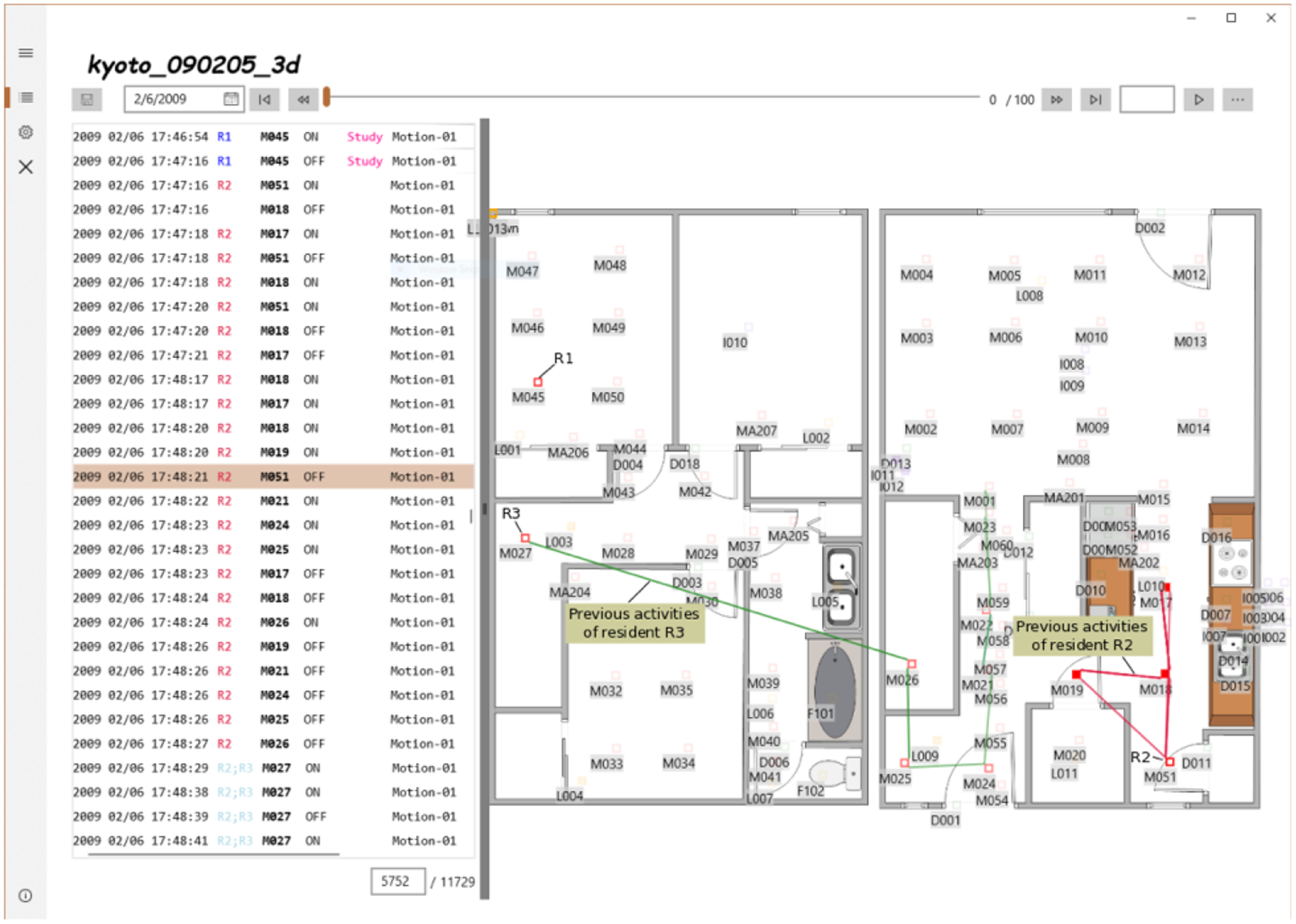
A screen shot of the ActViz annotation software used in this research to generate the ground truth of the association between sensor events and the residents in the smart home.

In sMRT, we first extract a sensor sequence by ignoring the deactivate messages, as shown in Table 2. Each sensor sequence entry is a two-tuple consisting of the sensor ID and the time when the sensor event is generated. By focusing on the activate messages, the sensor sequence captures the spatiotemporal relationships between the sensors deployed in the smart home. In a single resident environment, mutual information (MI) represents the likelihood that two sensors generate consecutive events [8] and thus quantizes the spatiotemporal relationship between sensors. In a multi-resident scenario, we assume that sensor pairs with a stronger MI relationship occur close to each other in the sensor event stream. As a result, we can estimate the MI of two sensors by mining the sensor co-occurrence.

TABLE 2.

Sensor sequence extracted from sensor messages shown in Table 1.

Time Tag	Sensor ID
02/06/2009 17:52:35	M025
02/06/2009 17:52:37	M045
02/06/2009 17:52:38	M025
02/06/2009 17:53:31	M024
02/06/2009 17:53:32	M019
02/06/2009 17:53:33	M021
02/06/2009 17:53:34	M018
02/06/2009 17:53:36	M051
02/06/2009 17:54:03	M051
02/06/2009 17:54:27	M045

Whenever a sensor is activated, we take a snapshot of the states of all sensors deployed in the smart home. Each active sensor in the snapshot represents an observation of a resident activity. Thus, we use the term sensor observation to refer to each active sensor in the snapshot. Table 3 shows a series of sensor observations extracted from the sensor messages in Table 1. Figure 3 demonstrates the relationship between sensor messages, sensor events and sensor observations. In the graph, each vertical grid line represents the time a sensor in the smart home is activated. The dots in the figure represent the sensor observations that are extracted from the sensor messages and the shaded rectangles represent a sensor being in the active state. The blue, red and green arrows in the figure connect the sensor observations into three sensor tracks associated with three residents (R1, R2, and R3, respectively). The figure shows that at any time step when the sensor observations are taken, a resident may be associated with multiple sensor events and a sensor event may be associated with multiple residents. Some sensor observations, such as sensors “I001” and “D012” in the figure, are not associated with any resident. In the context of resident tracking, we use the terms false alarms or clutter process to refer to sensor observations that are not associated with any resident. The goal of this work is to determine the number of residents in the home (3 during this time period) and to associate sensor events with the (three) corresponding tracks.

TABLE 3.

Sensor observations, recorded each time a sensor is activated.

Time Tag	Observation
02/06/2009 17:52:35	M025, I012, I011
02/06/2009 17:52:37	M045, I012, I011
02/06/2009 17:52:38	M045, M025, I012, I011
02/06/2009 17:53:31	M024, M025, I012, I011
02/06/2009 17:53:32	M019, M024, M025, I012, I011
02/06/2009 17:53:33	M021, M019, M024, M025, I012, I011
02/06/2009 17:53:34	M019, M018, M024, I012, I011
02/06/2009 17:53:36	M019, M051, M018, M024, I012, I011
02/06/2009 17:54:03	M051, I012, I011
02/06/2009 17:54:27	M045, M051, I012, I011

Fig. 3.

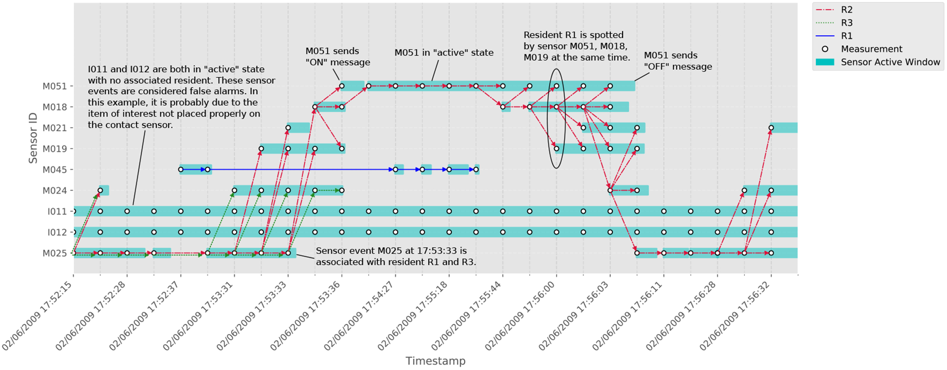
Multi-resident tracking graph showing the association between residents and sensor events and the relationship between sensor messages, sensor events and sensor observations. The figure is generated using the sensor messages recorded in the Kyoto dataset from the same time period as Tables 1–3. The arrows in the graph show the movement of all the active residents with respect to sensor observations.

4. sMRT: A Formal Framework of Multi-target Tracking

The objective of this research is to find a solution for multi-resident tracking (MRT) in smart homes with anonymous binary sensors that performs robustly in real homes with complex everyday behavior conditions. In addition to finding the association between sensor events and the corresponding residents, the proposed sMRT algorithm also estimates the number of active residents currently in the smart home and relaxes constraints of previous algorithms by not requiring additional information such as floor plans, sensor layouts, or resident-labeled training data.

We formulate the MRT problem as a sequential Bayes estimation (or filtering) problem in the framework of finite set statistics (FISST) [40]. We represent the state of each resident in the smart home as a random vector x that belongs to a state space $\mathcal{X}$. Thus, the state of all residents that are currently in the smart home at time step k can be modeled as a random finite set (RFS) $X_k=\left\{x_1,x_2,\dots ,x_n\right\}\in \mathcal{F}(\mathcal{X})$, where $\mathcal{F}(\mathcal{X})$ is the collection of all finite subsets of the state space $\mathcal{X}$. Each element x_i((1 ≤ i ≤ n) of the RFS X is a state vector of an active resident. The total number of active residents in the smart home, n (i.e., the cardinality |X_k| of the RFS X_k), is a random variable defined on ${\mathbb{Z}}_0^{+}$. Given a sequence of sensor events, sMRT calculates a Bayes optimal probability density, f(X_k), of the RFS X_k at time step k. The number of active residents, or the cardinality of the RFS X_k, is simultaneously derived.

To identify the relationship between the input (a series of sensor events) and the output (the probability density of the states of all active residents in the smart home), there are two challenges that we address. First, we will construct a dynamic model that predicts the state of each resident at the following time step given the current state. This dynamic model will serve as the corpus of information for the Bayes estimation process. The construction of such a dynamic model should be based solely on a series of recorded sensor events with no additional information that raises privacy concerns or is impractical to acquire for real homes. Second, we will derive a mathematically rigorous method to estimate the probability density of resident states and derive the association between each resident and sensor observations in real-time. sMRT addresses these challenges through two phases. First, a learning phase constructs the dynamic model by mining the co-occurrence of sensor events. Second, a tracking phase predicts the number of residents in the smart home as well as their association with the sensor events.

4.1. Learning Phase: Construction of Dynamic Model

In previous work, the dynamic model that encapsulates resident movement in a smart home was represented as a Markov chain, or a sensor graph, where the states of the Markov chain are mapped directly to the smart home sensors [33], [34]. In a smart home with q sensors, a total of q² transition matrix parameters, each representing the probability of a resident moving from one state (sensor location) to another, are estimated through counting [33],[34] or a conditional least squares method [35]. However, in those approaches, annotated sensor events and additional sensor layout information are required to make an accurate prediction. By mapping the states directly to sensors, these dynamic model would perform state prediction based solely on the current resident state without taking into account resident states in any of the previous steps.

In contrast, during the sMRT learning phase, we represent each sensor as a m × 1 vector in a m-dimensional space $\mathcal{Z}$. The space $\mathcal{Z}$. represents the measurement space. The dimensionality m of the measurement space is a hyper-parameter that can be chosen depending on the number and density of the sensors that are deployed in the smart home. The conditional probability of a resident transitioning from one sensor to another can be estimated using the distance between their vector representations in the measurement space $\mathcal{Z}$. In a smart home with q sensors, a total of q · m parameters must be estimated. Selecting m < q effectively injects dependencies between the conditional probabilities of a resident transiting between two sensors, a departure from earlier work in multi-resident tracking. By injecting these dependencies, a lesser amount of sensor data is needed to accurately learn the dynamic model parameters. Additionally, the model parameters are learned without the need for additional information such as the number of residents or sensor layout. With inspiration from word embedding used in natural language processing applications [41], we adopt a similar skip-gram model to leverage the co-occurrence of sensor events and train a generative model to learn the vector mapping between the sensors deployed in the smart home and the measurement space $\mathcal{Z}$. (see Section 4.1.1).

On the other hand, rather than mapping resident states directly to smart home sensors, we hypothesize that each resident’s movement can be represented as a point target maneuvering at constant velocity in the measurement space $\mathcal{Z}$. This hypothesis can be considered as a relaxation of the Markov assumption in sensor graphs, where the velocities along all m axes represent the information related to the resident states in all previous time steps and can be estimated during the tracking.

4.1.1. Sensor Vectorization

Consider a smart home where a total of q binary sensors (s₁, s₂, …, s_q) are deployed. Sensors s_i and s_j are adjacent if a resident can travel from s_i to s_j without triggering another sensor s_k (I ≠ j ≠ k). The goal of sensor vectorization is to find the corresponding vector representation $z_1,z_2,\dots ,z_q\in \mathcal{Z}$ such that if two sensors are adjacent (they can be activated in sequence without activating other sensors), they are mapped to two vectors close to each other in the measurement space. In other words, the closer z_i and z_j are, the higher is the conditional probability of triggering sensor s_i after sensor event s_j. As a result, we can further hypothesize that resident movement in the smart home is equivalent to a point target maneuvering in the measurement space.

In a smart home with a single resident, adjacent sensors always show up next to each other in the sensor sequence. In a multi-resident scenario, the recorded sensor sequence is a time-ordered collection of the active sensor messages associated with all residents in the smart home, possibly moving through different parts of the home. As a result, adjacent sensors are not necessarily next to each other in the sensor event sequence. However, they are more likely to show up within c sensor messages apart, where c is an integer that can be selected based on the expected number of smart home residents. Thus, we construct a generative model that predicts the probability of two sensors being adjacent parameterized by their vector representations in measurement space. This probability needs to fit the sensor pair’s co-occurrence observed in the recorded sensor sequence within a window of c sensor messages.

Formally, given a sensor sequence containing M sensor messages, ((t⁽¹⁾, s⁽¹⁾), …, (t^(M), s^(M))), where t⁽ⁱ⁾ is the time of the i^th sensor message and s⁽ⁱ⁾ is the corresponding sensor ID, we generate a training set where each sensor pair is observed within a window of c sensor messages in the sensor sequence, as shown in (1).

$$\mathit{\text{training set}}=\left\{\left(s^{(i)},s^{(j)}\right)|0<j-i\le c\right\}$$ (1)

We construct a generative model (as shown in Figure 4) that predicts the probability of a sensor pair, s and s′, being adjacent, denoted as P (s|s′) = P (s′|s). The training objective of the model is to map sensors s₁, …, s_q into vectors $z_1,\dots ,z_q\in \mathcal{Z}$ so that the average log likelihood $\mathcal{L}$, as shown in (2), is maximized in the training set.

$$\mathcal{L}=\frac{1}{M}\sum _{i=1}^M\sum _{0<j-i\le c}\text{log}P\left(s^{(j)}|s^{(i)}\right)$$ (2)

Fig. 4.

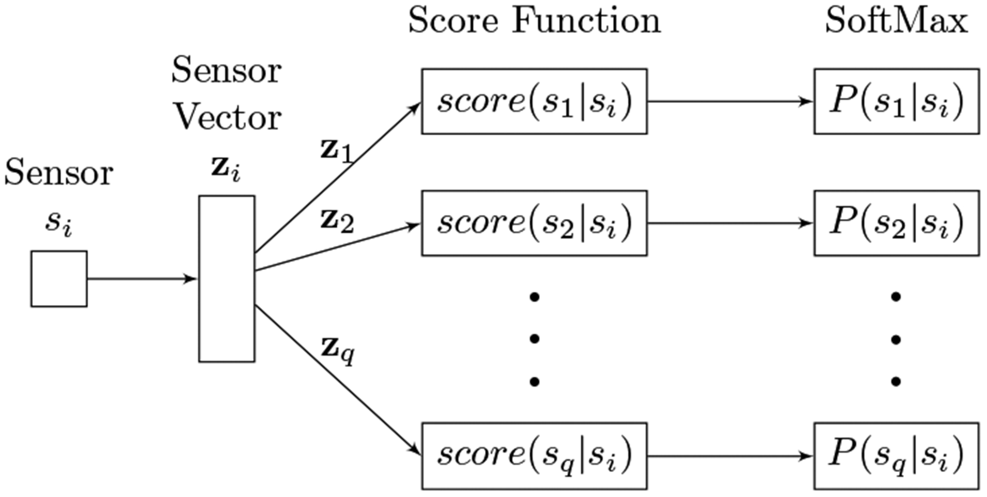
The generative model of sensor vectorization.

The probability of sensor s_i being adjacent to sensor s_j can be defined using a SoftMax function based on a score assigned to them, as shown in (3).

$$P\left(s_j|s_i\right)=\frac{exp\left(\mathit{\text{score}}\left(s_j|s_i\right)\right)}{{\sum }_{k=1}^{q}exp\left(\mathit{\text{score}}\left(s_k|s_i\right)\right)}$$ (3)

The score value score(s_j|s_i) needs to be larger when the distance between the corresponding vectors is smaller. We use a dot product as the similarity measure that defines the score function, as shown in (4).

$$\mathit{\text{score}}\left(s_j|s_i\right)=\mathit{\text{score}}\left(s_i|s_j\right)=z_i\cdot z_j^T$$ (4)

In a smart home containing a small number of sensors, the vector representations of sensors in the measurement space can be learned directly using SoftMax cross-entropy loss. To reduce the large computational cost of directly learning vector representations for a large number of sensors, noise contrast estimation (NCE) [42] is employed.

4.1.2. Linear Gaussian Dynamic Model

With each sensor in the smart home mapped into the measurement space, we use a constant velocity model of a point target maneuvering in the measurement space to approximate the movement of each resident in the smart home. The state vector of each resident is a (2m + 1) × 1 vector x = [x^T v^T r]^T, where x is an m × 1 vector representing the location of the resident in space $\mathcal{Z}$, v is an m × 1 vector representing the velocity of the resident, and r is an integer representing the resident ID. Given the state of the resident, x′, the resident state x at the next time step can be estimated using the linear equation as shown in (5). Here, F represents the linear motion multiplier, G represents the linear error multiplier, and w represents the velocity error.

$$x=F\cdot x^{\prime }+G\cdot w$$ (5)

If w can be modeled using a Gaussian distribution, the probability distribution of the resident state at the next time step can be expressed using a linear Gaussian model as in (6). Here, Q is the resulting covariance matrix. (The equation derivation is found in the supplemental material.)

$$f\left(x|x^{\prime }\right)=\mathcal{N}\left(x;F{x}^{\prime },Q\right)$$ (6)

Residents maneuver in the measurement space. Thus, sensor observations (represented by the corresponding sensor vectors) offer a noisy measurement of true resident states. If we assume that such measurement errors can be modeled as a Gaussian distribution with zero mean and a covariance matrix R, the relationship between a sensor observation z and the state vector x of the resident can be represented using a linear Gaussian model as shown in (7) with linear multiplier H.

$$f(z|x)=\mathcal{N}(z\text{;}H\cdot x,R)$$ (7)

Movement mapped from resident actual trajectories to the measurement space may not strictly follow the constant velocity assumption. However, with the help of the GM-PHD filter and track maintenance algorithm introduced in Section 4.2, errors between reality and the constant velocity assumption can be captured by the Gaussian noise in the dynamic and measurement models shown in (6) and (7). Thus, the GM-PHD filter can correct these errors based on new sensor observations obtained at each step.

4.2. Tracking Phase: GM-PHD Filter and Track Maintenance

During the tracking phase, a series of sensor observations is extracted from the sensor event stream by taking a snapshot of active sensors in the smart home every time a sensor is activated. Each active sensor is a measurement of a resident in the smart home. By replacing each active sensor with its vector representation in the measurement space, we define an observation set as $Z_k=\left\{z_1,\dots ,z_{n_z}\right\}$ at time step k, where n_z is the number of active sensors and each element z_i is the vector representation of the corresponding sensor. Among these n_z sensor observations, some are accurate measurements of active residents and some are false alarms (or clutter) due to communication errors or sensor failures. Alternatively, some residents may still be at home but may not be currently detected by the sensors. Thus, instead of creating a one-to-one mapping between each sensor observation and the corresponding resident, we also need to consider the possibilities of a new resident entering the home, an existing resident leaving the home, residents not being detected, sensor observations not being associated with any resident, and one-to-many or many-to-one associations between sensor observations and residents. The steps of the tracking phase are illustrated in Figure 5.

Fig. 5.

The sMRT tracking phase.

To model all of these possibilities, we use a Gaussian mixture probability density (GM-PHD) filter [43] that propagates the first-order moment of the multi-target probability density, or the probability hypothesis density (PHD), based on the dynamic and measurement models constructed during the learning phase. Additionally, we propose clustering-based track maintenance to associate the PHD predicted by the GM-PHD filter with resident identifiers to detect new residents while maintaining the traces of existing residents. Finally, each sensor observation, represented as a vector in the measurement space, is associated with the resident that is most likely to generate the observation.

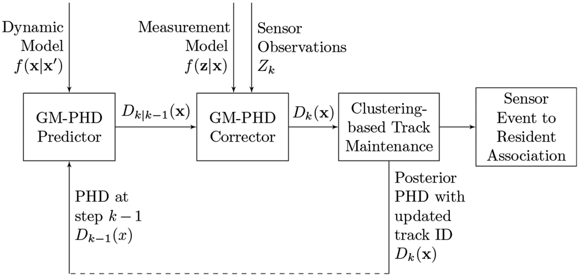
The GM-PHD filter is composed of a predictor and a corrector, as shown in Figure 5. Given the PHD of multiple residents at time step k − 1, D_k−1(x), the predictor estimates the multi-resident PHD at time step k, or D_k|k−1(x), based on the linear Gaussian dynamic model in (6). The corrector then refines the predicted PHD, D_k|k−1(x), based on the measurement model and sensor observations, Z_k. The output of the corrector is the Bayes optimal estimation of the posterior multi-resident PHD at time step k, D_k(x), which can be used to associate sensor events with residents in the smart home. If the multi-resident PHD at time step k − 1, D_k−1(x), is in the form of a Gaussian mixture, and the dynamic model and the measurement model are both linear Gaussian, the resulting posterior multi-resident PHD, D_k(x), is guaranteed to be in the form of a Gaussian mixture, as shown in (8), where J_k is the number of Gaussian components in the mixture and $w_k^{(i)}$, $m_k^{(i)}$ and $P_k^{(i)}$ are the weight, mean vector and covariance matrix of the i^th Gaussian component, respectively. (The derivation of (8) is included the supplementary material.)

$$D_k(x)=\sum _{i=1}^{J_k}{w}_k^{(i)}\mathcal{N}\left(x;m_k^{(i)},P_k^{(i)}\right)$$ (8)

Given the posterior PHD at time step k, we propose a clustering-based track maintenance algorithm that estimates the state of each resident, assigns identifiers to the newly-identified residents, and associates sensor observations with each resident based on the state probability distribution of each identified resident. According to the definition of PHD, the expected number of residents in the smart home can be calculated by integrating the PHD over the entire state space, as shown in (9).

$$N_k=\int \sum _{i=1}^{J_k}{w}_k^{(i)}\mathcal{N}\left(x;m_k^{(i)},P_k^{(i)}\right)dx=\sum _{i=1}^{J_k}{w}_k^{(i)}$$ (9)

We first assume that, at any time step, there is at most one newly-detected resident. Thus, during the predictor step, we can assign a new resident identifier to the resident ID field of the Gaussian mean state vectors for the target birth PHD. Given the measurement model and the dynamic model defined in Section 4.1.2, the resident identifier in the mean vector of each Gaussian component will remain unchanged while the Gaussian components are propagated in time through the GM-PHD filter. By grouping the Gaussian components that share the same resident identifier in the mean vector, the state probability distribution of each resident can be derived.

We now consider the case that multiple residents, $R_1^{(k)}\dots R_{n_r^{(k)}}^{(k)}$, enter the smart home at time k. As we assign a single resident identifier, r^(k), to all Gaussian components in the target birth PHD, the Gaussian components of the PHD, representing the states of all residents entering the smart home, share the same resident identifier r^(k). As the residents move through time, the cardinality of the PHD will eventually approximate the actual number of residents, N^(k), who enter the home. As a result, when tracking each resident $R_i^{(k)}$, the Gaussian components representing the PHD of those N^(k) residents need to be separated into N^(k) clusters with a unique resident identifier assigned to the Gaussian components for each cluster.

In sMRT, we introduce a clustering-based track maintenance algorithm that monitors the integral of the PHD associated with each resident identifier. The track maintenance algorithm is an iterative six-step process as follows.

1. Given the PHD with resident identifier r in the form of a Gaussian mixture as shown in (10), calculate the number of expected residents $N_{k,r}^{\prime }$ as shown in (11).

   $$D_{k,r}(x)=\sum _{i=1}^{J_{k,r}}{w}_{k,r}^{(i)}\mathcal{N}\left(x;m_{k,r}^{(i)},P_{k,r}^{(i)}\right)$$ (10)

   $$N_{k,r}^{\prime }=\lceil N_{k,r}-0.5\rceil =\lceil \sum _{i=1}^{J_{k,r}}{w}_{k,r}^{(i)}-0.5\rceil$$ (11)

2. Initialize the center of $N_{k,r}^{\prime }$ clusters randomly as ${\alpha }_1,\dots ,{\alpha }_{N_{k,r}^{\prime }}$.

3. For each cluster, find the Gaussian components in D_k,r(x) with the smallest distance between the mean of the Gaussian component and the center of the corresponding cluster. Assign those Gaussian components to the cluster so that the summation of the weights of all those Gaussian components does not exceed $N_{k,r}/N_{k,r}^{\prime }$. If there are Gaussian components left not assigned to any cluster, assign each of these to the nearest cluster determined by the distance between the center of the cluster and the mean of the Gaussian component.

4. Update the cluster center α_j to be the weighted mean of all Gaussian components assigned to the cluster, as shown in (12).

   $${\alpha }_j=\frac{1}{{\sum }_{i=1}^{J_{k,r,j}}{w}_{k,r,j}^{(i)}}\sum _{i=1}^{J_{k,r,j}}{w}_{k,r,j}^{(i)}{m}_{k,r,j}^{(i)}$$ (12)

   In (12), J_k,r,j represents the number of Gaussian components assigned to cluster j. The $w_{k,r,j}^{(i)}$, $m_{k,r,j}^{(i)}$ terms represent the weight and mean of those Gaussian components.

5. Repeat steps 3 and 4 until there are no further changes to the association between Gaussian components and clusters, or a maximum number of iterations is reached.

6. With the Gaussian components segregated into $N_{k,r}^{\prime }$ clusters, a new resident identifier is assigned to each cluster and is inserted into the resident ID field in the mean vector of each Gaussian component assigned to that cluster.

Finally, each sensor observation z_i ∈ Z_k is associated with the resident ID r so that the likelihood of producing the sensor observation z_i is maximized, as shown in (13).

$$\begin{gathered} r=\underset{r}{\text{argmax}}\int f\left(z_i|x\right)\sum _{i=1}^{J_{k,r}}{w}_{k,r}^{(i)}\mathcal{N}\left(x;m_{k,r}^{(i)},P_{k,r}^{(i)}\right)dx \\ =\underset{r}{\text{argmax}}\sum _{i=1}^{J_{k,r}}{w}_{k,r}^{(i)}\mathcal{N}\left(z;H{m}_{k,r}^{(i)},R+H{P}_{k,r}^{(i)}{H}^T\right) \end{gathered}$$ (13)

5. Evaluation of sMRT

To evaluate the performance of sMRT, we implement two other methods as baseline for comparison. The first method, denoted NN-sg, tracks the residents in the smart home using a sensor graph handcrafted according to the sensor layout of the smart home. The sensor graph, generated using the GR/ED method proposed by Crandall and Cook [33], determines the spatial adjacency between sensors. Whenever a new sensor message arrives, it is associated with an existing resident who was last spotted by an adjacent sensor. If no such resident can be found, the NN-sg method assumes that a new resident enters the space and a new resident identifier is assigned. On the other hand, if a resident has not been detected by any sensors for a period of 50 sensor events (this parameter is used by GR/ED [33]), the resident is assumed to have left the home or become “inactive”, and thus is removed from the list of existing residents. Unlike GR/ED, the NN-sg method only processes active sensors.

We also introduce a second method, denoted GNN-sg, as an alternative baseline method. GNN-sg further modifies the GR/ED algorithm. Specifically, GNN-sg uses a weighted directed sensor graph where the adjacency between any two sensors is determined manually according to the sensor layout in the smart home. Each weight, representing the probability of a resident triggering two sensors consecutively, is estimated from annotated sample data. The association between sensor observation and resident is determined using a global nearest neighbor method. At every time step, GNN-sg generates a list of all possible associations between sensor observations and all existing active residents. A score is assigned to each association hypothesis by accumulating the probabilities of each resident moving from the sensor location in previous time step to the new sensor location associated. The association with the highest score is selected and any sensor observation that is not associated with any resident is considered the start of a new resident track.

The objective of sMRT is to associate smart home sensor events with the residents who trigger them. To evaluate the ability of the algorithm to accomplish this task, we use the following two metrics to evaluate the performance of sMRT in comparison with the NN-sg and GNN-sg methods. First, we evaluate the association accuracy between sensor events and residents. An event association is considered correct if it matches the ground truth resident label.

Second, we evaluate whether the tracking algorithm correctly identifies the number of residents in the smart home. Evaluation is conducted using the TM004 and the Kyoto datasets introduced in Section 3. In the experiment, we require that each valid resident identifier be associated with at least three sensor events. In earlier activity recognition research, the shortest detectable activities contained at least three events (the “enter home” and “leave home” activities) [8]. Thus, if a resident identifier is associated with fewer than three sensor events, we consider those sensor events to be false alarms because those events are isolated incidents that are not related with any other sensors in the space. Because both GNN-sg and NN-sg use the physical sensor location in the smart home as a basis for building the sensor graph while sMRT uses an unsupervised sensor vectorization procedure to extract the spatiotemporal relationship between sensors from the unannotated sensor data directly, we expect GNN-sg and NN-sg to represent performance upper bounds for sMRT.

We define association accuracy as the fraction of total sensor events, D, in which the ground truth Y ⁽ⁱ⁾ equals the set of predicted resident IDsŶ⁽ⁱ⁾, as shown in (14). Resident IDs include the empty set (no resident) or a set of identifiers for one or more residents.

$$\mathit{\text{accuracy}}=\frac{1}{D}\sum _{i=1}^D\mathbf{1}\left(Y^{(i)}={\widehat{Y}}^{(i)}\right)$$ (14)

A second performance measure uses Hamming loss to give credits to partial matches between Y⁽ⁱ⁾ and Ŷ⁽ⁱ⁾. The definition of Hamming loss is shown in (15). In (15), N_R represents the total number of residents in the dataset.

$$\mathit{\text{hamming loss}}=\frac{1}{D}\cdot \frac{1}{N_R}\sum _{i=1}^D\sum _{j=1}^{N_R}\mathbf{1}\left(y_j^{(i)}={\widehat{y}}_j^{(i)}\right)$$ (15)

Moreover, if we focus on each resident that is annotated in the ground truth, we can also view sensor event to resident association as a binary classification problem. The two classes are events that are associated with a particular resident (+) and events not associated with that resident (−). In this approach, we can measure the precision, recall and F1-score for each resident.

The multi-label accuracy and Hamming loss values for both the TM004 and the Kyoto datasets are shown in Table 4. Performance using per-resident classification metrics for the TM004 and Kyoto datasets are shown in Tables 5 and 6, respectively. While macro averages are commonly reported when the classes are imbalanced, we are also interested in results on a per-datapoint bases. Thus, we provide micro and macro averages in Tables 5 and 6.

TABLE 4.

Multi-label accuracy and Hamming loss of sMRT, NN-sg and GNN-sg measured using the TM004 and Kyoto datasets. Best performance values are shown in bold. The best performance values that are statistically significant (p < 0.5) are marked with an asterisk.

Dataset	TM004			Kyoto
Methods	sMRT	NN-sg	GNN-sg	sMRT	NN-sg	GNN-sg
Accuracy	0.80	0.80	0.83*	0.76	0.82	0.86*
Hamming loss	0.08	0.09	0.07	0.18	0.11	0.07*
# Tracks	2834	569	1441	2266	330	969
# Sensor Events	51358			14409

TABLE 5.

Performance of sMRT, NN-sg and GNN-sg using the TM004 dataset, measured based on binary classification accuracy on a per-resident basis.

Metrics	Precision			Recall			F1-Score			# Events
Methods	sMRT	NN-sg	GNN-sg	sMRT	NN-sg	GNN-sg	sMRT	NN-sg	GNN-sg
R1	0.94	0.89	0.92	0.84	0.85	0.91	0.89	0.87	0.91	32272
R2	0.86	0.80	0.86	0.76	0.73	0.78	0.81	0.77	0.82	17873
R3	0.85	0.77	0.76	0.71	0.79	0.85	0.77	0.78	0.80	1202
R4	0.00	0.00	0.67	0.00	0.00	0.73	0.00	0.00	0.70	11
Average (Micro)	0.91	0.85	0.90	0.81	0.81	0.86	0.86	0.83	0.88	51358
Average (Macro)	0.66	0.61	0.80	0.58	0.59	0.82	0.62	0.60	0.81

TABLE 6.

Performance of sMRT, NN-sg and GNN-sg using the Kyoto dataset, measured based on binary classification accuracy on a per-resident basis.

Metrics	Precision			Recall			F1-Score			# Events
Methods	sMRT	NN-sg	GNN-sg	sMRT	NN-sg	GNN-sg	sMRT	NN-sg	GNN-sg
R1	0.74	0.92	0.91	0.72	0.83	0.94	0.73	0.88	0.93	5409
R2	0.65	0.83	0.90	0.79	0.91	0.94	0.71	0.87	0.92	6966
R3	0.68	0.76	0.82	0.59	0.53	0.75	0.63	0.62	0.78	2034
Average (Micro)	0.69	0.85	0.90	0.73	0.83	0.91	0.71	0.84	0.90	14409
Average (Macro)	0.69	0.84	0.88	0.70	0.76	0.88	0.69	0.79	0.88

For TM004, sMRT’s accuracy is 0.80, similar to the performance of NN-sg, and 0.03 lower than GNN-sg method. Using the Hamming loss metrics, sMRT scores 0.08, which is 0.01 better than the NN-sg method and 0.01 higher than the GNN-sg method. The Hamming loss of sMRT shows that only 8% of the associations are not identified by the sMRT algorithm. Unlike NN-sg and GNN-sg, the sMRT results are achieved without using annotated data or sensor topologies.

When we consider each separate resident in the TM004 dataset, as shown in Table 5, sMRT achieves a higher precision but a lower recall compared to the other two methods. Among the four residents labeled in the TM004 dataset, residents R1 and R2 are in the smart home most of the time, associated with 32,272 and 17,873 sensor events respectively. Residents R3 and R4 are likely visitors who trigger only 1,202 and 11 sensor events, respectively. However, the 11 sensor events associated with R4 are separated by sensor events triggered by other residents. As a result, those 11 sensor events are regarded as isolated sensor events by both NN-sg and sMRT and no resident identifier is produced.

However, in the Kyoto dataset where the sensors are more densely deployed with greater noise and less reliability, sMRT has a difficult time reliably tracking the residents compared to NN-sg and GNN-sg. By analyzing the sensor vectors learned by sMRT and the tracking results, we find that the main cause of the decrease in the performance of sMRT is that some sensors that are not physically adjacent to each other according to the sensor layout have a relatively short distance in the measurement space. The sensors exhibiting such an error either generate events only a few times in the dataset (recorded within 3 days) or have a higher probability of noise. For example, on one of the days, the bathroom door on the second floor was not closed properly, resulting in sensor D005 continually sending “OPEN” and “CLOSE” messages while another resident is downstairs in the living room triggering motion sensor M004. As a result, sMRT identifies sensors D005 and M004 as being close to each other in the measurement space while they are actually far from each other in the home.

Figures 6 and 7 show the accuracy and Hamming loss values of sMRT, NN-sg and GNN-sg when there are different numbers of residents in the smart home using the TM004 dataset. As the number of active residents in the smart home increases, the performances of sMRT and NN-sg decrease. However, baseline GNN-sg achieves a better accuracy when there are 4 resident in the smart home. One explanation for this anomaly is the small sample size for 4 residents. There are only 11 time steps when 4 residents are in the home, as shown in Table 5. In contrast, there are > 1, 000 sensor events for the other cases. According to the Hamming loss shown in Figure 7, we find that sMRT is more accurate in grouping the sensor events triggered by the same resident than NN-sg, though the performance is 0.01 lower than GNN-sg when there are two or three residents.

Fig. 6.

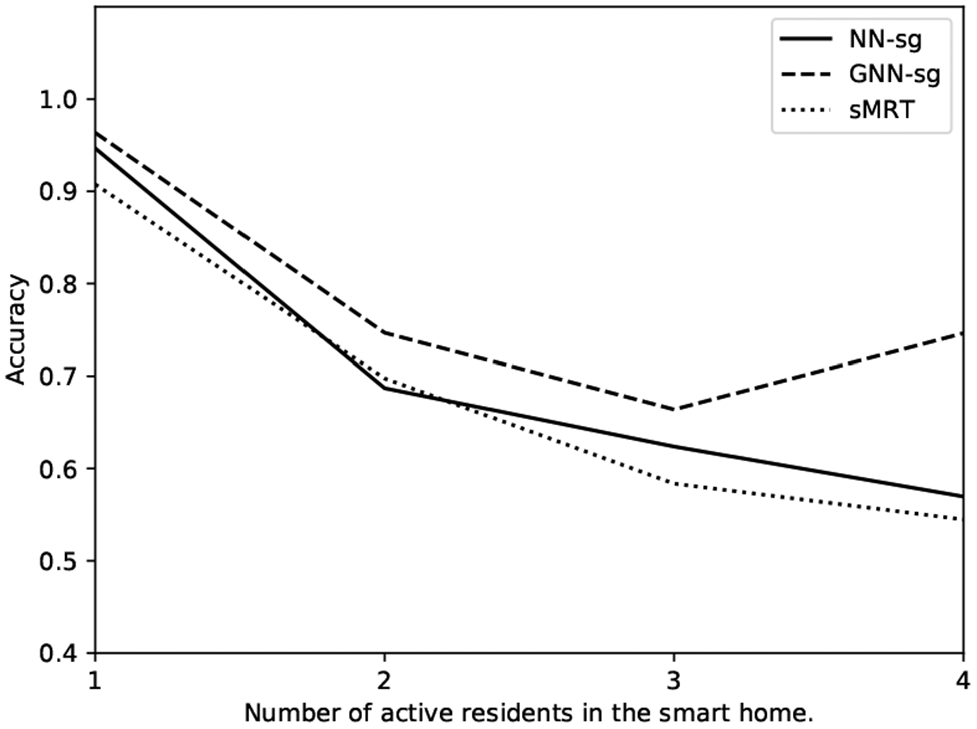
Accuracy score as a function of number of active residents for sMRT, NN-sg and GNN-sg using the TM004 dataset.

Fig. 7.

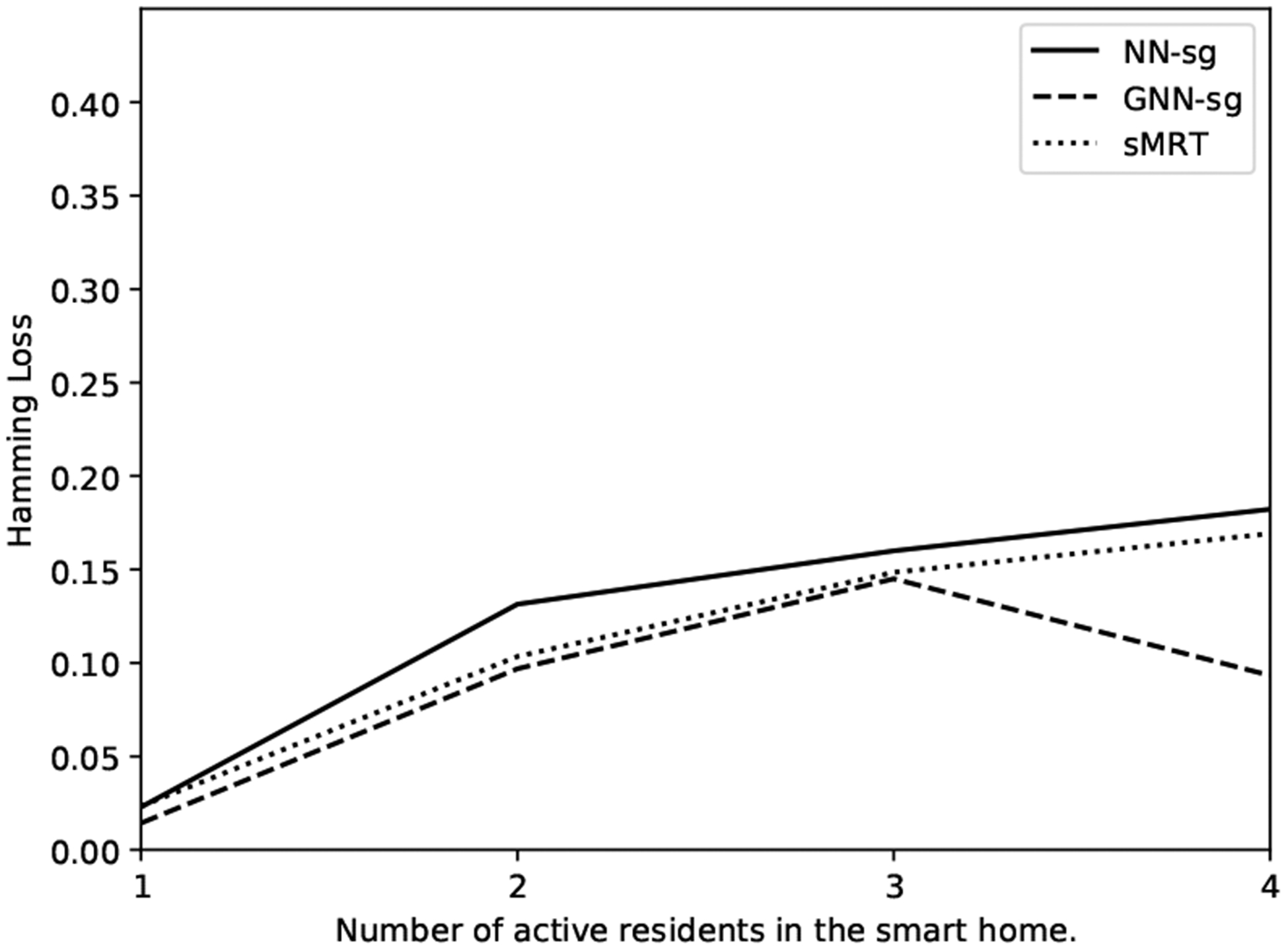
Hamming loss as a function of number of active residents for sMRT, NN-sg and GNN-sg using the TM004 dataset.

We also evaluate these methods based on their ability to estimate the number of active residents currently present in the smart home. In earlier multi-resident tracking research, a resident is considered to be inactive if the resident has not been detected by any sensors for over 100 seconds, or 50 consecutive sensor events on average [33]. Since sMRT and both baseline methods operate based on discrete time steps, we count an existing resident as active when a sensor event is triggered within the next 50 time steps. This rule is applied to both the ground truth and the result of NN-sg to determine the number of active residents in the smart home. In the case of sMRT, the likelihood of a resident being active at any time step, or present in the home, can be calculated by integrating the PHD distribution as shown in (9). If the likelihood > 0.5, we consider the resident to be active.

Table 7 shows the average absolute value of the error between the number of active residents identified by three candidate algorithms and the ground truth. As indicated by these results, both the sMRT and NN-sg methods, on average, are accurate for resident cardinality estimation as the average errors of both methods are smaller than 1, while GNN-sg generates a higher number of resident identifiers and fails to estimate the number of active residents as accurately as the other methods.

TABLE 7.

Average error of sMRT, NN-sg and GNN-sg in estimation of the number of active residents in the smart homes. Best performance values are shown in bold. The best performance values that are statistically significant (p < 0.5) are marked with an asterisk.

Dataset	TM004			Kyoto
Methods	sMRT	NN-sg	GNN-sg	sMRT	NN-sg	GNN-sg
Average Error	0.59	0.41*	1.27	0.85	0.63*	4.56

Ideally, we want the sensor events associated with the same residents to match the resident identifier predicted by the tracking algorithm. However, in the experiments, we find the segmentation errors, where the sensor events that are associated with the same resident are split into multiple tracks with different resident identifiers, may affect the real-life performance when the tracking algorithm is used for activity-aware applications. By counting the number of valid resident identifiers generated by each method, as shown in Table 4, both sMRT and GNN-sg results in a higher number of valid resident identifiers compared to the NN-sg method. The result indicates that both sMRT and GNN-sg tend to generate more resident identifiers and associate the sensor events that are triggered by same resident associated with those identifiers.

During the propagation of PHD in sMRT, a one-to-one relationship between sensor observations and residents is still assumed. sMRT handles the many-to-one relationship between sensor observations and residents by properly setting the parameters for the clutter process, namely λ_c and c(z). These two parameters serve as counterweights to prevent the rapid increase of cardinality estimation when a resident triggers two sensor observations at the same time. However, when a resident is at a location where the sensors are more densely populated, the chances that a many-to-one association between sensor observations and residents may be higher than what the clutter process parameters can handle. As a result, sMRT will spawn a new resident track. Not long afterward, the original track may terminate itself. The behavior of sMRT may thus lead to a higher count of valid resident identifiers while still maintaining an accurate estimation of the number of active residents in the smart home. However, adjacent sensor events that are associated to the same resident are likely to still be adjacent, even when a new resident identifier is assigned.

In contrast, the segmentation errors observed for GNN-sg are caused by keeping multiple resident identifiers valid at the same time. In similar cases where a resident is spotted by multiple sensor observations, GNN-sg simultaneously creates multiple resident identifiers associated with each of those sensor observations. Based on the GNN policy, the sensor events are separated into different tracks in an interleaved fashion. It is more likely, compared to sMRT, that the adjacent sensor events associated with the same resident are assigned to different resident identifiers. This behavior causes an increase in the predicted number of valid resident identifiers and an inaccurate estimation of the number of active residents in the smart home. Moreover, even though GNN-sg results in a better accuracy and Hamming loss score (i.e., GNN-sg is more accurate in grouping the sensor events triggered by same resident together), the result is less effective in activity-aware applications where the continuity of sensor events is an important factor.

In a multi-resident smart home, the assumption of one-to-one associations between sensor events and residents may not hold, especially when multiple residents are performing joint activities and are moving together as a group (e.g., cooking together). Even though all of the tracking algorithms assume a one-to-one association, differences in enforcing this assumption results in different levels of tracking capabilities for joint-activity scenarios. Both baseline methods, NN-sg and GNN-sg, treat the one-to-one association as a rule. Therefore, if multiple residents trigger the activation of the same sensor, the algorithms can only associate the sensor observation to one of the residents. In cases when multiple residents are performing joint activities in a local area, GNN-sg will generate additional parallel tracks, leading to an over-estimation of the number of active residents in the smart home as shown in Table 7. In contrast, even though sMRT does not explicitly model joint activities, it predicts the sensor they will next jointly trigger through sensor vectorization in combination with a constant velocity model. As a result, sMRT can track resident joint activity in a local space. However, in the case of multiple residents moving together, e.g. going downstairs together to the kitchen in the morning, the performance of sMRT depends on the length of the sequence when residents move together. Since sMRT’s corrector is derived based on the assumption that there is a one-to-one association between sensor observation and resident, the integral of the PHD corresponding to each resident (i.e., the sum of weights of Gaussian components associated with each resident) will decrease. However, as there is still a sensor observation during the procedure and both residents are likely to be associated with the sensor observation, the sum of weights of both residents will decrease but their sum will still reach1. Thus, when the multiple residents go separate ways, the PHD integral of each resident may still be higher than the birth PHD and the tracks identified by the sMRT algorithm can be maintained.

Finally, we compare the computational complexity of sMRT and the baseline algorithms. NN-sg associates each existing resident with the nearest or most-likely sensor observation. Given n sensor observations, and N currently-active residents, NN-sg’s worst case runtime is O (nN). GNN-sg attempts to find the best one-to-one assignment between sensor observations and existing residents. Using an efficient method such as the Hungarian algorithm, this could be accomplished in time O(n³). The sMRT tracking is composed of a GM-PHD filter track and a clustering-based maintenance algorithm. Assuming a maximum of J Gaussian components in the mixture and a m-dimensional measurement space, GM-PHDO updating bounded by is O (nJm³). The worst-case complexity of sMRT’s track maintenance is O (N Jmi), where i is the number of iterations that lead to clustering convergence.

6. Conclusion

In this work, we introduce the sMRT algorithm that solves the multi-resident tracking problem in smart homes equipped with anonymous binary sensors. sMRT contrasts with previous work by learning the spatiotemporal relationship between sensors using un-annotated sensor data recorded. We evaluate the performance of sMRT using two smart home datasets recorded in real-life settings with human-annotated ground truth of associations between each sensor events and the residents living in the smart home. The performance of sMRT is compared with two other methods, NN-sg and GNN-sg, that rely on a provided sensor layout, smart home floor plan, and annotated sensor data.

The results support our hypothesis that sMRT is capable of tracking multiple residents with similar accuracy to the methods that are provided with additional information. sMRT can also provide a rough estimation of the number of active residents in the smart home. However, the performance of sMRT depends on the reliability of sensors that are deployed in the smart home and the accuracy of the sensor events that are recorded, as the recorded sensor data is the only source of information. The other limitation of sMRT is the higher possibility of segmentation errors when tracking residents in a location where sensors are comparatively more densely deployed.

In the future, sMRT can be refined by exploring alternatives to the simple constant velocity model presented in this paper so that a better accuracy can be achieved in predicting the next sensor event a resident will trigger. Moreover, further investigation can focus on analyzing the placement, spatial coverage and density of ambient sensors in the smart home and their impact on multi-resident tracking.

Biographies

Tinghui Wang was born in China in 1988. He received the B.E. degree in Microelectronics from Shanghai Jiaotong University, Shanghai, China. In 2009. He joined Digilent Inc, China Office and Beecube Inc, China Office after graduation. He is currently pursuing the Ph.D. in electrical and computer engineering at Washington State University. His current research involves activity recognition, multi-target tracking in smart home environments with binary sensors.

Diane J. Cook is a Huie-Rogers Chair Professor at Washington State University. She received her Ph.D. in computer science from the University of Illinois and her research interests include machine learning, pervasive computing, and designed of automated strategies for health monitoring and intervention. She is an IEEE Fellow and a Fellow of the National Academy of Inventors.

References

- [1].Mekonnen AA and Lerasle F, “Comparative evaluations of selected tracking-by-detection approaches,” IEEE Trans. Circuits Syst. Video Technol, vol. 29, no. 4, pp. 996–1010, April 2019. [Google Scholar]
- [2].Nayak NM, Zhu Y, and Roy Chowdhury AK, “Hierarchical graphical models for simultaneous tracking and recognition in wide-area scenes,” IEEE Trans. Image Process, vol. 24, no. 7, pp. 2025–2036, July 2015. [DOI] [PubMed] [Google Scholar]
- [3].Choi W and Savarese S, “Understanding collective activitiesof people from videos,” IEEE Trans. Pattern Anal. Mach. Intell, vol. 36, no. 6, pp. 1242–1257, June 2014. [DOI] [PubMed] [Google Scholar]
- [4].Brdiczka O, Crowley JL, and Reignier P, “Learning situation models in a smart home,” IEEE Trans. Syst., Man, Cybern. B, vol. 39, no. 1, pp. 56–63, 2009. [DOI] [PubMed] [Google Scholar]
- [5].Gochoo M, Tan T, Liu S, Jean F, Alnajjar FS, and Huang S, “Unobtrusive activity recognition of elderly people living alone using anonymous binary sensors and DCNN,” IEEE J. Biomed. Health Inform, vol. 23, no. 2, pp. 693–702, March 2019. [DOI] [PubMed] [Google Scholar]
- [6].Rafferty J, Nugent CD, Liu J, and Chen L, “From activity recognition to intention recognition for assisted living within smart homes,” IEEE Trans. Human-Mach. Syst, vol. 47, no. 3, pp. 368–379, 2017. [Google Scholar]
- [7].Gayathri KS, Easwarakumar KS, and Elias S, “Probabilistic ontology based activity recognition in smart homes using Markov logic network,” Knowledge-Based Syst, vol. 121, pp. 173–184, 2017. [Google Scholar]
- [8].Krishnan NC and Cook DJ, “Activity recognition on streaming sensor data,” Pervasive and Mobile Computing, vol. 10, pp. 138–154, 2014. [DOI] [PMC free article] [PubMed] [Google Scholar]
- [9].Cook DJ, “Learning setting-generalized activity models for smart spaces,” IEEE Intell. Syst, vol. 27, no. 1, pp. 32–38, 2012. [DOI] [PMC free article] [PubMed] [Google Scholar]
- [10].Minor BD, Doppa JR, and Cook DJ, “Learning activity predictors from sensor data: Algorithms, evaluation, and applications,” IEEE Trans. Knowl. Data Eng, vol. 29, no. 12, pp. 2744–2757, 2017. [DOI] [PMC free article] [PubMed] [Google Scholar]
- [11].Suryadevara NK, Mukhopadhyay SC, Wang R, and Rayudu RK, “Forecasting the behavior of an elderly using wireless sensors data in a smart home,” Eng. Appl. Artificial Intell, vol. 26, no. 10, pp. 2641–2652, 2013. [Google Scholar]
- [12].Minor B, Doppa JR, and Cook DJ, “Data-driven activity prediction: Algorithms, evaluation methodology, and applications,” in Proc. ACM SIGKDD Int. Conf. Knowledge Discovery Data Mining ACM, 2015, pp. 805–814. [Google Scholar]
- [13].Aramendi AA, Weakley A, Goenaga AA, Schmitter-Edgecombe M, and Cook DJ, “Automatic assessment of functional health decline in older adults based on smart home data,” J. Biomedical Informatics, vol. 81, pp. 119–130, 2018. [DOI] [PMC free article] [PubMed] [Google Scholar]
- [14].Akl A, Snoek J, and Mihailidis A, “Unobtrusive detection of mild cognitive impairment in older adults through home monitoring,” IEEE J. Biomed. Health Inform, vol. 21, no. 2, pp. 339–348, 2017. [DOI] [PMC free article] [PubMed] [Google Scholar]
- [15].Liu L, Stroulia E, Nikolaidis I, Miguel-Cruz A, and Rincon AR, “Smart homes and home health monitoring technologies for older adults: A systematic review,” Int. J. Medical Informatics, vol. 91, pp. 44–59, 2016. [DOI] [PubMed] [Google Scholar]
- [16].Austin J, Dodge HH, Riley T, Jacobs PG, Thielke S, and Kaye J, “A smart-home system to unobtrusively and continuously assess loneliness in older adults,” IEEE J. Transl. Eng. Health Med, vol. 4, pp. 1–11, 2016. [DOI] [PMC free article] [PubMed] [Google Scholar]
- [17].Hagler S, Austin D, Hayes TL, Kaye J, and Pavel M, “Unobtrusive and ubiquitous in-home monitoring: A methodology for continuous assessment of gait velocity in elders,” IEEE Trans. Biomed. Eng, vol. 57, no. 4, pp. 813–820, 2010. [DOI] [PMC free article] [PubMed] [Google Scholar]
- [18].Arcelus A, Jones MH, Goubran R, and Knoefel F, “Integration of smart home technologies in a health monitoring system for the elderly,” in Advanced Information Networking and Applications Workshops, 2007, AINAW’07. 21st International Conference on, vol. 2. IEEE, 2007, pp. 820–825. [Google Scholar]
- [19].Dawadi PN, Cook DJ, Schmitter-Edgecombe M, and Parsey C, “Automated assessment of cognitive health using smart home technologies,” Technol. Health Care, vol. 21, no. 4, pp. 323–343, 2013. [DOI] [PMC free article] [PubMed] [Google Scholar]
- [20].Schmitter-Edgecombe M, Cook DJ, Weakley A, and Dawadi P, “Using smart environment technologies to monitor and assess everyday functioning and deliver real-time intervention,” Role Technol. Clinical Neuropsychology, p. 293, 2017. [Google Scholar]
- [21].Dahmen J, Thomas BL, Cook DJ, and Wang X, “Activity learning as a foundation for security monitoring in smart homes,” Sensors, vol. 17, no. 4, p. 737, 2017. [DOI] [PMC free article] [PubMed] [Google Scholar]
- [22].Aran O, Sanchez-Cortes D, Do M-T, and Gatica-Perez D, “Anomaly detection in elderly daily behavior in ambient sensing environments,” in Int. Workshop Human Behavior Understanding Springer, 2016, pp. 51–67. [Google Scholar]
- [23].Ordóñez FJ, de Toledo P, and Sanchis A, “Sensor-based Bayesian detection of anomalous living patterns in a home setting,” Personal and Ubiquitous Computing, vol. 19, no. 2, pp. 259–270, 2015. [Google Scholar]
- [24].Ahmadi-Karvigh S, Ghahramani A, Becerik-Gerber B, and Soibelman L, “Real-time activity recognition for energy efficiency in buildings,” Applied Energy, vol. 211, pp. 146–160, 2018. [Google Scholar]
- [25].Park H, Hwang S, Won M, and Park T, “Activity-aware sensor cycling for human activity monitoring in smart homes,” IEEE Commun. Lett, vol. 21, no. 4, pp. 757–760, April 2017. [Google Scholar]
- [26].De Paola A, Ferraro P, Gaglio S, Re GL, and Das SK, “An adaptive bayesian system for context-aware data fusion in smart environments,” IEEE Trans. Mobile Comput, vol. 16, no. 6, pp. 1502–1515, June 2017. [Google Scholar]
- [27].Thomas BL and Cook DJ, “Activity-aware energy-efficient automation of smart buildings,” Energies, vol. 9, no. 8, p. 624, 2016. [Google Scholar]
- [28].Corno F and Razzak F, “Intelligent energy optimization for user intelligible goals in smart home environments,” IEEE Trans. Smart Grid, vol. 3, no. 4, pp. 2128–2135, December 2012. [Google Scholar]
- [29].Wilson DH and Atkeson C, “Simultaneous tracking and activity recognition (STAR) using many anonymous, binary sensors,” in Pervasive Computing. Berlin, Heidelberg: Springer, 2005, pp. 62–79. [Google Scholar]
- [30].Hsu K-C, Chiang Y-T, Lin G-Y, Lu C-H, Hsu JY-J, and Fu L-C, “Strategies for inference mechanism of conditional random fields for multiple-resident activity recognition in a smart home,” in Int. Conf. Ind. Eng. Other Appl. Appl. Intell. Syst Springer, 2010, pp. 417–426. [Google Scholar]
- [31].Crandall AS and Cook DJ, “Attributing events to individuals in multi-inhabitant environments,” in 2008 IET 4th Int. Conf. Intell. Environments, July 2008, pp. 1–8. [Google Scholar]
- [32].Crandall AS and Cook DJ, “Coping with multiple residents in a smart environment,” J. Ambient Intell. Smart Environments, vol. 1, no. 4, pp. 323–334, 2009. [Google Scholar]
- [33].Crandall AS and Cook DJ, “Tracking systems for multiple smart home residents,” in Human Behavior Recognition Technologies: Intelligent Applications for Monitoring and Security. Hershey, PA: IGI Global, 2011, pp. 111–129. [Google Scholar]
- [34].Müller SM and Hein A, “Multi-target data association in binary sensor networks for ambulant care support,” Int. J. Advances Networks Services, vol. 9, no. 1 & 2, pp. 20–29, 2016. [Google Scholar]
- [35].Ghasemi V and Pouyan AA, “Modeling users data traces in multi-resident ambient assisted living environments,” Intl. J. Computational Intell. Syst, vol. 10, no. 1, pp. 1289–1297, 2017. [Google Scholar]
- [36].Amri M-H, Becis Y, Aubry D, Ramdani N, and Fränzle M, “Robust indoor location tracking of multiple inhabitants using only binary sensors,” in 2015 IEEE Int. Conf. Automation Sci. Eng. (CASE), Aug 2015, pp. 194–199. [Google Scholar]
- [37].Song L and Wang Y, “Multiple target counting and tracking using binary proximity sensors: Bounds, coloring, and filter,” in Proc. ACM Int. Symp Mobile Ad Hoc Networking Computing ACM, 2014, pp. 397–406. [Google Scholar]
- [38].De D, Song W-Z, Xu M, Wang C-L, Cook D, and Huo X, “FindingHuMo: Real-time tracking of motion trajectories from anonymous binary sensing in smart environments,” in 2012 IEEE 32nd Int. Conf. Distributed Computing Syst., June 2012, pp. 163–172. [Google Scholar]
- [39].Wang C, De D, and Song W-Z, “Trajectory mining from anonymous binary motion sensors in smart environment,” Knowledge-Based Syst, vol. 37, pp. 346–356, 2013. [Google Scholar]
- [40].Goodman IR, Mahler RP, and Nguyen HT, Mathematics of data fusion. Springer Science & Business Media, 2013. [Google Scholar]
- [41].Pennington J, Socher R, and Manning CD, “Glove: Global vectors for word representation,” in Empirical Methods in Natural Language Processing (EMNLP), 2014, pp. 1532–1543. [Google Scholar]
- [42].Gutmann M and Hyvärinen A, “Noise-contrastive estimation: A new estimation principle for unnormalized statistical models,” in Proc. Int. Conf. Artificial Intell. Statist, 2010, pp. 297–304. [Google Scholar]
- [43].Vo B-N and Ma W-K, “The Gaussian mixture probability hypothesis density filter,” IEEE Trans. Signal Process, vol. 54, no. 11, pp. 4091–4104, 2006. [Google Scholar]
Associated Data
This section collects any data citations, data availability statements, or supplementary materials included in this article.