Abstract
The dendritic spines play a crucial role in learning and memory processes, epileptogenesis, drug addiction, and postinjury recovery. The shape of the dendritic spine is a morphological key to understand learning and memory process. The classification of the dendritic spines is based on their shapes but the major questions are how the shapes changes in time, how the synaptic strength changes, and is there a correlation between shapes and synaptic strength? Because the changes of the classes by dendritic spines during activation are time dependent, the forward-directed autoregressive hidden Markov model (ARHMM) can be used to model these changes. It is also more appropriate to use an ARHMM directed backward in time. Thus, the mixture of forward-directed ARHMM and backward-directed ARHMM (MARHMM) is used to model time-dependent data related to the dendritic spines. In this article, we discuss (1) how to choose the initial probability vector and transition and dependence matrices in ARHMM and MARHMM for modeling the dendritic spines changes and (2) how to estimate these matrices. Many descriptors to classify dendritic spines in two-dimensional or/and three-dimensional (3D) are available. Our results from sensitivity analysis show that the classification that comes from 3D descriptors is closer to the truth, and estimated transition and dependence probability matrices are connected with the molecular mechanism of the dendritic spines activation.
Keywords: ARHMM, classification, dendritic spines, machine learning, MARHMM
1. Introduction
Dendritic spines are short protrusions that harbor excitatory synapses, which are believed to play a major role in neuronal plasticity and integration through their structural reorganization (Yuste and Denk, 1995; Segal, 2002; Xu et al., 2009). Many physiological and pathological phenomena rely on brain plasticity, including learning and memory, epileptogenesis, drug addiction, and postinjury recovery. Their peculiar shape suggests that spines can serve as an autonomous postsynaptic compartment that isolates chemical and electrical signaling. How neuronal activity modifies the morphology of the spine and how these modifications affect synaptic transmission and plasticity are intriguing issues. Thus, the dendritic spine shape has been accepted for determining the strength of the synaptic connections and is thought to underlie the processes of information coding and memory storage in the brain. Indeed, the induction of long-term potentiation (LTP) or long-term depression is associated with the enlargement or shrinkage of the spine, respectively (Bosch and Hayashi, 2012).
Classification of dendritic spines, according to their shape and size, is a popular strategy to evaluate maturation and pathological changes of neurons. Spines are often classified into four morphological classes: filipodia, thin, stubby, and mushroom (Peters and Kaiserman-Abramof, 1970). It must be noted, however, that the existing categorization of dendritic spine shapes does not provide a clear definition of each group. Some researchers prefer to add two additional categories: branched and cup-shaped spines (Harris and Kater, 1994; Hering and Sheng, 2001). An important question is whether the categorization of spines according to their morphology represents a rigid classification of distinct entities or tentative labeling of transient spine states. Live-cell imaging studies clearly show that spines are very dynamic and undergo reversible transformation between thin and mushroom morphologies in a time scale of minutes to hours (Fischer et al., 1998).
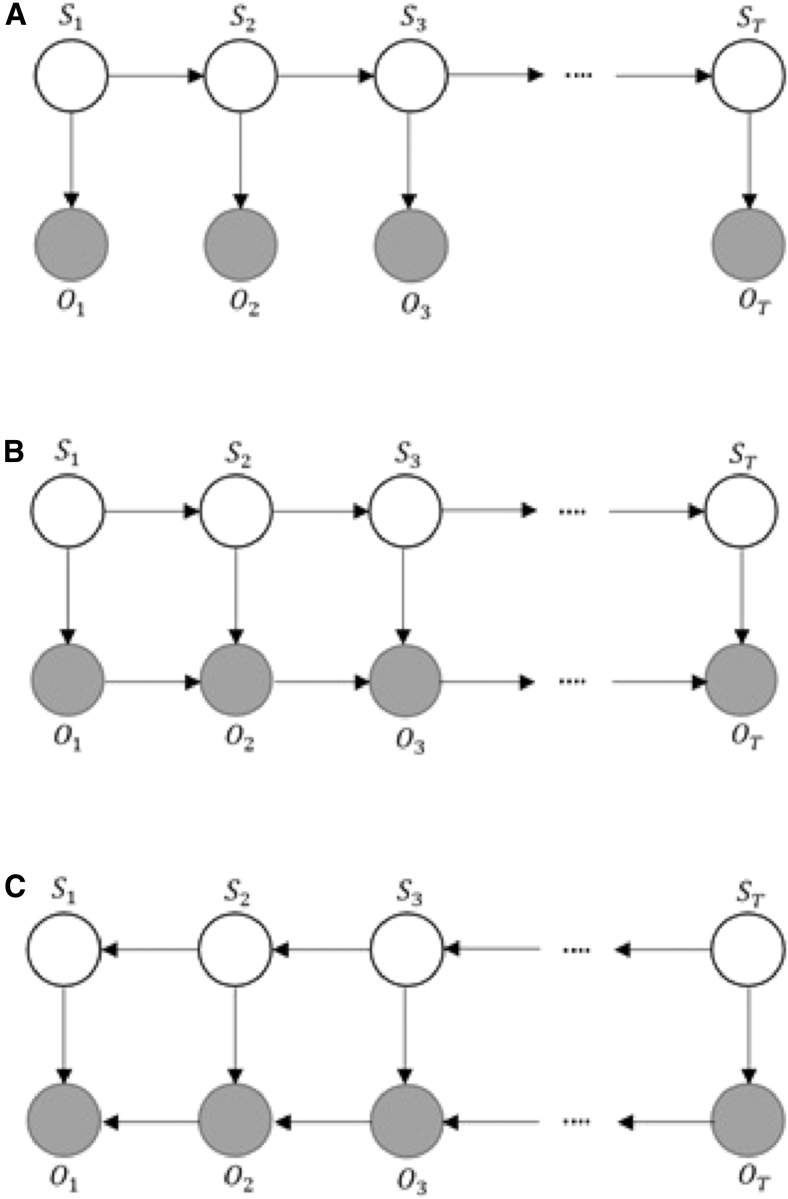
Another important question is how the changes of the shapes of the dendritic spines in time correlate with learning and memory process—is there a correlation between changes of the class of the dendritic spines and changes of the enlargement or shrinkage of the spine and changes with the synaptic strength. Another very important question is how to build a model based on the population of dendritic spines including their classification changes, synaptic strength, learning, and memory process. These questions can help us find answers to better understand the process of learning and memory and how the synaptic plasticity process works. Several neuromorphological tracing tools are available to segment and classify spines in two-dimensional (2D) and/or three-dimensional (3D). The major problem is determining which descriptors in 2D or 3D give the most accurate classification (by accurate classification we mean stable classification of dendritic spines, highest prediction accuracy, and highest biological relevance). Because of the dynamic changes of dendritic spine shapes (and, therefore, its class) in time, we should use time-dependent statistical models to answer for this problem. One of the most important models used in statistics and machine learning is hidden Markov model (HMM), which was described by Rabiner (1989) and Rabiner and Juang (1993). Figure 1A shows a sequence of states (S) and observations (O) for first-order HMM (where sequence of states is S = and sequence of observations is ).
FIG. 1.
(A) Graphical model for first-order conventional HMM. (B) Graphical model for a first-order forward-directed ARHMM. (C) Graphical model for a first-order backward-directed ARHMM. S means state, O means observation. This figure is taken from Rezaei Tabar et al. (2019). HMM, hidden Markov model; ARHMM, autoregressive HMM.
A first-order HMM instantiates two simplifying assumptions. First, as with a first-order Markov chain, the probability of a particular state depends only on the previous state:
| (1) |
Second, the probability of an output observation Oi depends only on the state that produced the observation Si and not on any other states or any other observations:
| (2) |
Unfortunately, HMM can be poor at capturing dependency between observations because of the statistical assumptions it makes. In many situations, the assumption that observation has a common effect in another observation in the future simplifies the design of the Bayesian network: directed arcs should flow forward in time. The extensions of the HMM called autoregressive HMM (ARHMM) and mixture ARHMM (MARHMM) (Fig. 1B, C) are used especially for time series data (Rezaei Tabar et al., 2019). The ARHMM can be calculated as the forward-directed ARHMM encourages correlation among observations by adding direct dependencies between them. By adding direct dependencies between observations, samples drawn from forward-directed ARHMM are thus smoother than samples from an HMM, usually making a better generative model in time series problems (Stanculescu et al., 2014; Rezaei Tabar et al., 2019). The forward-directed ARHMM is a Bayesian network and obeys the following two conditional independence relations:
| (3) |
Using these conditional independence relations, the joint distribution of a sequence of states and observations can be included as follows:
| (4) |
The backward-directed ARHMM is also known as a Bayesian network. According to D-separation concept in Bayesian network, the backward-directed ARHMM also has the following two conditional independence relations:
| (5) |
The same way, forward-directed ARHMM also has the following two conditional independence relations:
| (6) |
Also we can define the forward and backward algorithms that are to find out a recursive way to represent the variable sequence in both models. The forward probability represents the probability of the observation sequence up to time t and the state k at time t, given model (or ) as the following formulas:
| (7) |
| (8) |
For some stochastic processes, it may be more appropriate to use an ARHMM directed backward in time (Rezaei Tabar et al., 2019). The backward probability represents the probability of the partial observation sequence from to the end, given state k at time t as follows:
| (9) |
| (10) |
In Equations (7)–(10), and are set of parameters where = (the transition matrix, the initial emission matrix, the emission matrix, and vector of initial state).
Note that the index L − R is timestamp from left to right for representing the forward-directed ARHMM and R − L is timestamp from right to left for representing the backward-directed ARHMM.
For MARHMM, equation describing the model is as follows:
| (11) |
where and are the probability of the observation sequences given the forward-directed ARHMM and backward-directed ARHMM, respectively, and and are mixing weights such that and . can be computed by obtained the Baum–Welch algorithm.
The ARHMM and MARHMM parameters are estimated by the expectation-maximization (EM) algorithm (Rezaei Tabar et al., 2019). The algorithm arises in many computational biology applications that involve probabilistic models, and it also enables parameter estimation in probabilistic models with incomplete data. The EM algorithm computes probabilities for each possible completion of the missing data, using the current parameters. These probabilities are used to create a weighted training set consisting of all possible completions of the data. Finally, a modified version of maximum likelihood estimation that deals with weighted training examples provides new parameter estimates (McLachlan and Krishnan, 2007). By using weighted training examples rather than choosing the single best completion, the EM algorithm accounts for the confidence of the model in each completion of the data (Chuong and Batzoglou, 2008). In the rest of the article, we refer to a population of spines stimulated by LTP as dynamic data.
2. Data Preparation
Details about data preparation are described in Bokota et al. (2016) in section “Data preparation and analysis.” Here we describe only the differences in chemical substances that were used in experiments in dynamic data sets gathered at three time points. In this experiment, the chemical LTP was induced through the application of bath in a mixture of 50 μM forskolin, 50 μM picrotoxin, and 0.1 μM rolipram [each dissolved in dimethyl sulfoxide (DMSO)] in a maintenance medium. Subsequently, experiment was obtained from three points in time (timestamps): control (timestamp t0), 10 minutes after stimulation (timestamp ), and 40 minutes after stimulation (timestamp ).
3. Methods
Details about all four descriptors that were used to classify dendritic spines are given in Supplementary Data S1. In Supplementary Data S2, details about how we prepare the data and how the vectors and matrices should look like to run the code are described. Classification of the dendritic spines in all three timestamps was done by four descriptors. Two descriptors were used for 2D classification and two were used for 3D classification. A Viterbi algorithm that was used in machine learning is also described in Supplementary Data (Supplementary Data S1).
In Matlab (The MathWorks, 2018), we implemented the ARHMM and MARHMM algorithms, whereas Viterbi analysis was conducted in R in version 3.4 in HMM package (Development, 2010). We took dendritic spines marked by SpineMagick descriptor (Ruszczycki et al., 2012) and marked the same dendritic spines using 2D programs (2dSpAn and Spinetools) and 3D programs (3dSpAn and Neurolucida 360). Depending on the descriptor we were working on, dendritic spines were classified as stubby, filipodia, mushroom, thin, and long (combining filipodia and thin into one class) and “not existing” (i.e., after stimulation we observed that these spines did not exist anymore—this class represents spines that were absorbed by the neuron). Finally, we proceed to run the descriptor using the following parameters: data, level, transition probability matrix, initial probability vector, number of iterations, and dependence matrix As an output, the algorithm produces an estimated transition probability matrix, estimated emission probability matrix, and logarithm of probability (logarithm of likelihood) at each iteration. Also, we use methods such as principal component analysis (Jolliffe, 2002), fuzzy partition coefficient, and hierarchical clustering by k-means the same way as by Bokota et al. (2016) and Urban et al. (2019)—the results and comments are described in Supplementary Data S3.
4. Results
In this section, we describe the sensitivity analysis results of MARHMM and machine learning for various combinations of the parameters: initial probability vector, transition probability matrix, and dependence probability matrix, different values. We also show how the changes in synaptic strength over time depend on the changes in the area surface (for 2D descriptors) or volume (for 3D descriptors). Also, we show that differences in transition probabilities between states in time depend on 2D or 3D classification.
4.1. Sensitivity analysis—initial probability vector
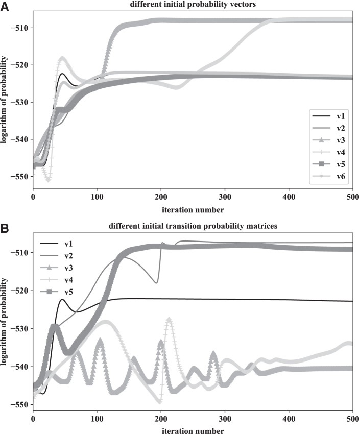
To show the impact of different initial probability vectors for the same data, we prepare six versions of the initial probability vector with a level equal to 3. We use the same transition probability matrix and dependence matrix in all six situations. Table 1 gives versions of initial probability vectors. Results of our experiment with the initial probability vector are presented in Figure 2A. We can see that version 3 (v3 in legend, gray triangle line) is better than other curves—convergence is achieved after ∼150 iterations, and the value of the logarithm of probability is lowest. In addition, version 4 (v4 in legend, light gray vline) is also good but converges only after ∼370 iterations. The remaining versions have inferior performance.
Table 1.
Vectors Used in Sensitivity Analysis for Initial Probability
| Version no. | Vector |
|---|---|
| Version 1 | [0.3;0.4;0.3] |
| Version 2 | [0.5;0.2;0.3] |
| Version 3 | [0.8;0.1;0.1] |
| Version 4 | [0.2;0.7;0.1] |
| Version 5 | [0.2;0.2;0.6] |
| Version 6 | [0.4;0.4;0.2] |
FIG. 2.
(A) Results for different initial probability vectors for the same data, transition probability matrix, and dependence matrix. (B) Results for different transition probability matrices for the same data, initial probability vector, and dependence matrix.
4.2. Sensitivity analysis—transition probability matrix
To show the impact of different input transition probability matrices for the same data, we prepare five versions of the transition probability matrix with level = 3, initial probability vector was the same in all five situations, the same with dependence matrix. Table 2 gives versions of transition probability matrices. The results are shown in Figure 2B. We can see that version 5 (v5 in legend, square dark gray line) is better than other tested versions because it converges quicker (the line representing the logarithm of probability is stable after ∼150 iterations) and has a smaller value (i.e., higher probability) than the others versions. The version 2 (v2 in legend, dark gray line) performs similarly, but more iterations are required to have convergence (∼210). Version 1 (v1 in legend, black line) converges very quickly (∼110 iterations) but it has visibly worse quality. Versions 4 and 3 (v4 [light gray vline] and v3 [triangle gray line] in the legend) have some oscillations and show intermediate quality. The estimated transition probability matrix for version 5 is given in Supplementary Data S4.
Table 2.
Matrices Used in Sensitivity of Analysis for Initial Transition Probability
| Version no. | Matrix |
|---|---|
| Version 1 | |
| Version 2 | |
| Version 3 | |
| Version 4 | |
| Version 5 |
4.3. Sensitivity analysis—dependence matrix
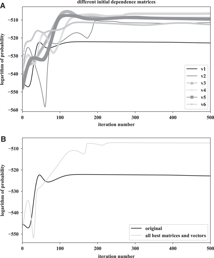
To show the impact of different dependence matrices for the same data, we prepare six versions of the dependence matrix with a level equal to 3. We use the same transition probability matrix and the initial probability vector in all six situations. Table 3 gives versions of dependence probability matrices that were used. The results are shown in Figure 3A. We can see that both version 4 (v4 in legend, light gray vline) and version 3 (v3 in legend, triangle gray line) are good. In triangle gray line after ∼150 iterations, the line is stable but in the opposite, to the triangle gray line, the light gray vline has less value of the logarithm of probability. The versions 5, 2, and 6 (v5 [square dark gray line], v2 [dark gray line], and v6 [gray dotted line] in legend) have similar performances. The worst version is 1 (v1 in legend, black line). The estimated dependence probability matrix for version 4 is given in Supplementary Data S3.
Table 3.
Matrices Used in Sensitivity Analysis for Initial Dependence Probability
| Version no. | Matrix |
|---|---|
| Version 1 | |
| Version 2 | |
| Version 3 | |
| Version 4 | |
| Version 5 | |
| Version 6 |
FIG. 3.
(A) Results for different dependence matrices for the same data, initial probability vector, and transition probability matrix. (B) Difference between choosing the best matrices and vectors than choosing it randomly. We used the same data for both lines.
4.4. Autoregressive hidden Markov model
Based on the results from Sections 4.1 to 4.3, we plot the curve for the best matrices and vectors and plot the curve for random matrices and vectors (but not the best). Figure 3B shows that after choosing random matrices and vectors, our logarithm of probability is on the level of −523 after 125 iterations. The curve that was a plot with the best matrices and vectors has logarithm of probability on level −505 after 215 iterations. That means is better to make more iterations and have better results (). Here, of course, the difference is not so big, but in other data, the difference can be bigger and can give wrong information.
4.5. Sensitivity analysis— in MARHMM
The application of the MARHMM method is similar to the ARHMM. The only difference is that we must also give initial values of mixture coefficients ( and ). Figure 4A shows the results of the different values (eight situations) for the same data set and the number of iterations as the ARHMM methods used in the previous Sections 4.1–4.4. The transition probability matrix, initial probability vector, and dependence matrix were the same. Table 4 gives versions of values used in MARHMM. Figure 4A shows that version 4 (light gray vline for and ) has a lower value of the logarithm of probability than the rest versions. For the other versions, the value of is higher, and on a similar level to each other.
FIG. 4.
(A) Results for different values for the same data, transition probability matrix, initial probability vector, and dependence matrix. (B) Logarithm of the probability for different descriptors 2D and 3D for segmentation and classification of dendritic spines into one of the classes. 2D, two-dimensional; 3D, three-dimensional.
Table 4.
Values Used in Sensitivity Analysis in Mixture Autoregressive Hidden Markov Model
| Version no. | Values |
|---|---|
| Version 1 | = 0.5, = 0.5 |
| Version 2 | = 0.4, = 0.6 |
| Version 3 | = 0.3, = 0.7 |
| Version 4 | = 0.2, = 0.8 |
| Version 5 | = 0.1, = 0.9 |
| Version 6 | = 0.6, = 0.4 |
| Version 7 | = 0.8, = 0.2 |
| Version 8 | = 0.9, = 0.1 |
4.6. The Viterbi algorithm
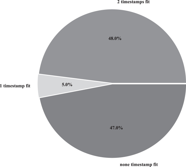
The Viterbi algorithm was used in machine learning—first our data were split into two sets: set for training (100 spines) and for the test (200 spines). We use the transition and emission probability matrices calculated by MARHMM (Supplementary Data S3). Results of our test were verified by the Viterbi algorithm. Figure 5 shows the percentage of situations in which the algorithm found all three or two/one/none of the classifications of dendritic spines (our aim was not to construct a predictive model, but to show how on time-dependent data after using MARHMM, we can use results in machine learning).
FIG. 5.
Results for machine learning for the most probable path.
4.7. Relationship between spine shape and synaptic strength
We know that the synaptic strength is correlated with the area of the dendritic spine—from 2D descriptors, we have a parameter that is called area. In 3D descriptors instead of the area we have volume parameter that will also help us in showing changes in synaptic strength. For each dendritic spine that exists in all three timestamps, we check how the area or volume changes. We focus on five situations:
-
I
n time the area/volume is growing.
-
I
n time the area/volume is decreasing.
-
I
n time the area/volume is not changing.
-
I
n time the area/volume is growing and then decreasing.
-
I
n time the area/volume is decreasing and then growing.
Table 5 gives results for two 2D descriptors (for area parameter) and for one 3D descriptor (for volume parameter). We check what kind of classes exist in different situations, and unfortunately we did not find here any correlation (e.g., in all five situations, we could find few [two or three] dendritic spines that in all three timestamps were classified as stubby).
Table 5.
Changing of the Dendritic Spines Synaptic Strength in Time, Calculated by Different Descriptors
| Synaptic strength situation | 2dSpAn (%) | Spinetools (%) | 3dSpAn (%) |
|---|---|---|---|
| Growing | 14.65 | 12.72 | 27.86 |
| Decreasing | 23.13 | 22.54 | 4.96 |
| Not changing | 0 | 0 | 0 |
| Growing and decreasing | 34.52 | 31.63 | 44.65 |
| Decreasing and growing | 27.68 | 33.1 | 22.52 |
4.8. Probabilistic model
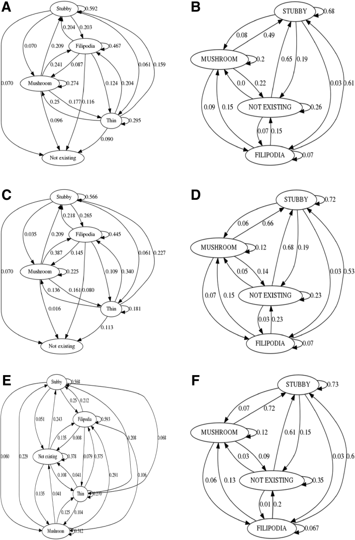
Figure 6A shows the results for 2D and 3D descriptors with the different number of classes (details about the matrices and vectors used to plot the curves are described with details given in Supplementary Data S2 and also results for estimated emission and transition probability matrix are given in Supplementary Data S3). Based on the information that classification in 3D of the dendritic spines with four classes is better than other 3D classifications, we calculate transition matrix [it was calculated the same way as by Urban et al. (2019)] in section “Transition matrix.” Figure 6 shows results for transition matrices for three situations (transitions between t0 and , t0 and , and and ) for 3D (based on 3dSpAn classification) and 2D classifications from Urban et al. (2019). The first difference is that in 3D, we do not have thin class (in 3dSpAn there are equations for each dendritic spine that can be classified as thin, but in our data, we did not match it). Second difference is in probabilities between classes, we can observe that some probabilities from 2D and 3D are the same or very close, especially in transition from time stamp t0 to time stamp (e.g., transition probability for dendritic spine classified as stubby changes to mushroom will be in 3D 0.09 and in 2D it will be 0.07). In transitions between time t0 and and between and , we could not find probabilities that will be very similar/close. This probability values between dendritic spine classes can be used in building network [e.g., our probabilities can be used in model from Barrett et al. (2009)].
FIG. 6.
(A,C,E) Probabilistic model from Urban et al. (2019); (B,D,F) Probabilistic model built on MARHMM results where (A) and (B) are time stamp t0, (C) and (D) are time stamp , and (E) and (F) are time stamp t40. MARHMM, mixture ARHMM.
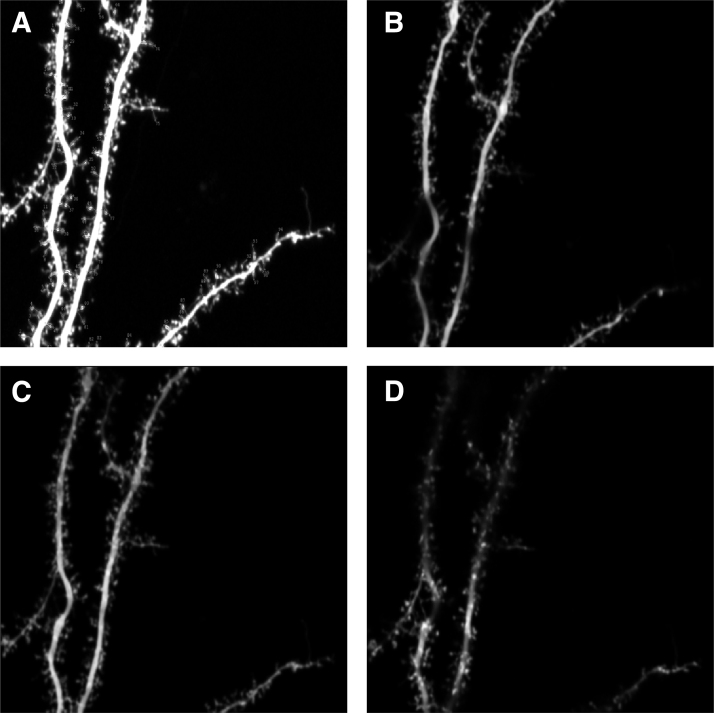
As we expected, the classification that comes from 3D descriptor is closer to the truth than a 2D descriptor. In 3D, we have more information about dendritic spine location: we know the location on the neuron (x- and y-axis) and also we have a third axis (z-axis) that shows us how the spines change depending on depth. In 2D, we do not have z-axis and because of this, we do not know exactly how the spine looks like. For example, in 2D we could see spine that looks like one big mushroom spine, but in 3D it was not one big dendritic spine, but two or three spines and depend on z-axis depth (Fig. 7). Table 6 gives the example of classification, using all the descriptors (mentioned and described in Supplementary Data S1), for the same dendritic spine. In this case, 2D descriptor gives us wrong classification and occasionally designates artifacts as dendritic spines (which are not dendritic spines—when we check it in 3D, or on another program [such as ImageJ] in which we can change point of view by changing the z-axis, thanks to it we can see how dendritic spines change during the depth on the neuron).
FIG. 7.
Example of neuron with dendritic spines. (A) 2D view but without z-axis. (B–D) 2D view with z-axis (for each subplot z-axis has different value).
Table 6.
Classification for the Same Dendritic Spine After Using Different Programs in Three Timestamps
| t0 | t10 | t40 | |
|---|---|---|---|
| 2dSpAn | M | T | F |
| Spinetools | M | M | M |
| dSpAn | S | S | S |
| Neurolucida 360 | M | M | M |
F, filipodia; M, mushroom; S, stubby; T, thin.
After showing results of the sensitivity analysis (Sections 4.1–4.3 and 4.5), it should be more clear and also how important it is to choose property matrices and/or vectors and what kind of curves to avoid. This knowledge is very important because it depends on what we put to the program will have different values of the estimated transition and dependence probability matrices as output. Figure 3B shows the difference between using all the best matrices and vectors than using random values.
As given in Table 5, results from 3D descriptors are different than those from 2D descriptors. One of the explanations of this is that the structure of the dendritic spines is tightly correlated with their function and reflects the synapse properties. At the cellular level, the most extensively studied aspect of this phenomenon is related to dendritic spine enlargement in response to stimulation (Kasai et al., 2003; Rangamani et al., 2016). Synapse strengthening or weakening along with dendritic spine formation and elimination assures correct processing and storage of the incoming information in the neuronal network.
Based on the results from estimated transition probability matrix and dependence probability matrix from 3dSpAn classification with four classes (Supplementary Data S3), we can multiply each probability from estimated dependence probability matrix by a number of spines—thanks to it we have a number of dendritic spines from each class from each timestamp. About changes, dendritic spines from one class to another MARHMM is unfortunately not good. This is because the estimated transition probability matrix is our hidden states (they are responsible for timestamps in our experiment), in estimated dependence matrix we have only information about the class (column) and timestamp (row). To build a probability model based on classification changes in time, we need, for example, some graph models (Stefanini, 2014). Of course, based on the estimated transition probability matrices, we can observe that the probabilities are the biggest between timestamps t0 and and between and , which is equivalent to changes in the dendritic spines dynamics after activation of the molecular mechanisms (Kasai et al., 2003; Szepesi et al., 2014).
Based on our results, we can support the hypothesis of Bokota et al. (2016), that the biological information is not stored in the spine shapes or sizes depending on their classes but is rather related to the dynamic changes at the spine population level.
5. Conclusion
The structure of the dendritic spines is tightly correlated with their function and reflects the synapse properties. Synapse strengthening or weakening along with dendritic spine formation and elimination assures correct processing and storage of the incoming information in the neuronal network. This plastic nature of the dendritic spines allows them to undergo activity-dependent structural modifications, which are thought to underlie learning and memory formation. At the cellular level, the most extensively studied aspect of this phenomenon is related to dendritic spine enlargement in response to stimulation (Bokota et al., 2016). The presented methods can be used not only in dendritic spines for neurobiological experiments but also in other biological branches [genetics (Kröger et al., 2017), molecular biology (Qing, 2017), immunology (Hill et al., 2017), hematology (Efficace et al., 2017)], or even in other science problems such as in medicine (diagnostic, epidemiologic) (Porcelli and Guidi, 2015; DasMahapatra et al., 2017), psychology (psychology diagnostic) (Porcelli and Guidi, 2015), or sociology (relationships between people) (Wong et al, 2017). In each instance in which we want to know about the next step, we can use the forward-directed ARHMM, if we want to know about the previous step, we can use backward-directed ARHMM, and finally the MARHMM can be used for considering both previous and next steps. Also results from MARHMM used in machine learning can be used in developing a new spice classification descriptor. Also based on results from MARHMM, we can choose the best descriptor, and by using other tools we try to build probabilistic models.
Supplementary Material
Ethics Statement
All experimental procedures were carried out in accordance with the ethical committee on animal research of the Nencki Institute, based on the Polish Act on Animal Welfare and other national laws that are in full agreement with the EU directive on animal experimentation.
Authors' Contributions
P.U. and V.R.T. conceived the project and performed the analysis based on data from experiments. P.U., M.D., G.B., and V.R.T. prepared the figures and wrote the article. N.D. aided in 3D segmentation of dendritic spines using the 3DSpAn descriptor. D.P. and S.B. were supervising the project and conducted extensive discussions during our analysis. All authors read and approved the final article.
Author Disclosure Statement
The authors declare they have no conflicting financial interests.
Funding Information
This study was supported by the Polish National Science Center (Grant No. 2014/15/B/ST6/05082), Foundation for Polish Science (TEAM to D.P.), and by the grant from the Department of Science and Technology, India, under Indo-Polish/Polish-Indo project no.: DST/INT/POL/P-36/2016. The study was cosupported by Grant No. 1U54DK107967-01 “Nucleome Positioning System for Spatiotemporal Genome Organization and Regulation” within 4DNucleome NIH program. S.B. was funded by Department of Biotechnology grant (Grant No. BT/PR16356/BID/7/596/2016).
Supplementary Material
References
- The ARHMM and MARHMM source codes are available at https://bitbucket.org/4dnucleome.marhmm
- Barrett A.B., Billings G.O., Morris R.G.M., et al. 2009. State based model of long-term potentiation and synaptic tagging and capture. PLoS Comput. Biol. 5, 1–12 [DOI] [PMC free article] [PubMed] [Google Scholar]
- Bokota G., Magnowska M., Kuśmierczyk T., et al. 2016. Computational approach to dendritic spine taxonomy and shape transition analysis. Front. Comput. Neurosci. 10, 2–3 and 9–10 [DOI] [PMC free article] [PubMed] [Google Scholar]
- Bosch M., and Hayashi Y.. 2012. Structural plasticity of dendritic spines. Curr. Opin. Neurobiol. 22, 383–388 [DOI] [PMC free article] [PubMed] [Google Scholar]
- Chuong B.D., and Batzoglou S.. 2008. What is the expectation maximization algorithm? Nat. Biol. 26, 897–899 [DOI] [PubMed] [Google Scholar]
- DasMahapatra P., Raja P., Gilbert J., et al. 2017. Clinical trials from the patient perspective: Survey in an online patient community. BMC Health Serv. Res. 17, 166. [DOI] [PMC free article] [PubMed] [Google Scholar]
- Development S.S. 2010. HMM: Hidden Markov Models. Scientific Software Development. Dr. Lin Himmelmann/HMM-HiddenMarkovModel.package.HMM
- Efficace F., Gaidano G., and Lo-Coco F.. 2017. Patient-reported outcomes in hematology: Is it time to focus more on them in clinical trials and hematology practice? Blood 130, 859–866 [DOI] [PubMed] [Google Scholar]
- Fischer M., Kaech S., Knutti D., et al. 1998. Rapid actin-based plasticity in dendritic spines. Neuron 20, 847–854 [DOI] [PubMed] [Google Scholar]
- Harris K.M., and Kater S.B.. 1994. Dendritic spines: Cellular specializations imparting both stability and flexibility to synaptic function. Annu. Rev. Neurosci. 17, 341–371 [DOI] [PubMed] [Google Scholar]
- Hering H., and Sheng M.. 2001. Dendritic spines: Structure, dynamics and regulation. Nat. Rev. Neurosci. 2, 880–888 [DOI] [PubMed] [Google Scholar]
- Hill D.A., Dudley J.W., and Spergel J.M.. 2017. The prevalence of eosinophilic esophagitis in pediatric patients with IgE-mediated food allergy. J. Allergy Clin. Immunol. 5, 369–375 [DOI] [PMC free article] [PubMed] [Google Scholar]
- Jolliffe I.T. 2002. Principal component analysis and factor analysis, 150–166. In Principal Component Analysis. Springer Verlag; New York, New York, NY [Google Scholar]
- Kasai H., Matsuzaki M., Noguchi J., et al. 2003. Structure stability function relationships of dendritic spines. Trends Neurosci. 26, 360–368 [DOI] [PubMed] [Google Scholar]
- Kröger N., Panagiota V., Badbaran A., et al. 2017. Impact of molecular genetics on outcome in myelofibrosis patients after allogeneic stem cell transplantation. Biol. Blood Marrow Transpl. 23, 1095–1101 [DOI] [PubMed] [Google Scholar]
- McLachlan G., and Krishnan T.. 2007. The EM algorithm and extensions fundamentals. In Applied Probability & Statistics, vol. 382. John Wiley & Sons, New York, NY [Google Scholar]
- Peters A., and Kaiserman-Abramof I.R.. 1970. The small pyramidal neuron of the rat cerebral cortex. The perikaryon, dendrites and spines. Am. J. Anat. 127, 321–355 [DOI] [PubMed] [Google Scholar]
- Porcelli P., and Guidi J.. 2015. The clinical utility of the diagnostic criteria for psychosomatic research: A review of studies. Psychother. Psychosom. 5, 265–272 [DOI] [PubMed] [Google Scholar]
- Qing C. 2017. The molecular biology in wound healing & non-healing wound. Chin. J. Traumatol. 20, 189–193 [DOI] [PMC free article] [PubMed] [Google Scholar]
- Rabiner L.R. 1989. A tutorial on hidden Markov models and selected applications in speech recognition. Proc. IEEE 77, 257–286 [Google Scholar]
- Rabiner L.R., and Juang B.H.. 1993. Fundamentals of speech recognition, 321–390. In Prentice-Hall Signal Processing Series. Prentice Hall PTR, Englewood Cliffs, New Jersey
- Rangamani P., Levy M.G., Khan S., et al. 2016. Paradoxical signaling regulates structural plasticity in dendritic spines. Proc. Natl. Acad. Sci. 113, 5298–5307 [DOI] [PMC free article] [PubMed] [Google Scholar]
- Rezaei Tabar V., Fathipor H., Perez S.H., et al. 2019. Mixture of forward-directed and backward-directed autoregressive hidden Markov models for time series modeling. J. Iran. Stat. Soc. 18, 139–162 [Google Scholar]
- Ruszczycki B., Szepesi Z., Wilczynski G.M., et al. 2012. Sampling issues in quantitative analysis of dendritic spines morphology. BMC Bioinformatics 13, 213. [DOI] [PMC free article] [PubMed] [Google Scholar]
- Segal M. 2002. Release of calciumform stores alters themorphology of dendritic spines in cultured hippocampal neurons. Progr. Brain Res. 138, 53–59 [Google Scholar]
- Stanculescu I., Williams C.K., and Freer Y.. 2014. Autoregressive hidden Markov models for the early detection of neonatal sepsis. IEEE J. Biomed. Health Inf. 18, 1560–1570 [DOI] [PubMed] [Google Scholar]
- Stefanini F.M. 2014. Chain graph models to elicit the structure of a Bayesian network. Sci. World J. 2014, 749150. [DOI] [PMC free article] [PubMed] [Google Scholar]
- Szepesi Z., Hosy E., Ruszczycki B., et al. 2014. Synaptically released matrix metalloproteinase activity in control of structural plasticity and the cell surface distribution of GluA1-AMPA receptors. PLoS ONE 9 [DOI] [PMC free article] [PubMed] [Google Scholar]
- The MathWorks. 2018. Matlab Software
- Urban P., Rezaei Tabar V., Bokota G., et al. , 2019. Dendritic spines taxonomy: The functional and structural classification • Time-dependent probabilistic model of neuronal activation. J. Comput. Biol. 26, 1–14 [DOI] [PMC free article] [PubMed] [Google Scholar]
- Wong A., Chau A.K.C., Fang Y., et al. 2017. Illuminating the psychological experience of elderly loneliness from a societal perspective: A qualitative study of alienation between older people and society. Int. J. Environ. Res. Public Health 14, 824. [DOI] [PMC free article] [PubMed] [Google Scholar]
- Xu T., Xinzhu Y., Perlik A.J., et al. 2009. Rapid formation and selective stabilization of synapses for enduring motormemories. Nature 462, 915–919 [DOI] [PMC free article] [PubMed] [Google Scholar]
- Yuste R., and Denk W.. 1995. Dendritic spines as basic functional units of neuronal integration. Nature 375, 682–684 [DOI] [PubMed] [Google Scholar]
Associated Data
This section collects any data citations, data availability statements, or supplementary materials included in this article.


