Three-dimensional MRI Bone Models of the Glenohumeral Joint Using Deep Learning: Evaluation of Normal Anatomy and Glenoid Bone Loss

Abstract

Purpose

To use convolutional neural networks (CNNs) for fully automated MRI segmentation of the glenohumeral joint and evaluate the accuracy of three-dimensional (3D) MRI models created with this method.

Materials and Methods

Shoulder MR images of 100 patients (average age, 44 years; range, 14–80 years; 60 men) were retrospectively collected from September 2013 to August 2018. CNNs were used to develop a fully automated segmentation model for proton density–weighted images. Shoulder MR images from an additional 50 patients (mean age, 33 years; range, 16–65 years; 35 men) were retrospectively collected from May 2014 to April 2019 to create 3D MRI glenohumeral models by transfer learning using Dixon-based sequences. Two musculoskeletal radiologists performed measurements on fully and semiautomated segmented 3D MRI models to assess glenohumeral anatomy, glenoid bone loss (GBL), and their impact on treatment selection. Performance of the CNNs was evaluated using Dice similarity coefficient (DSC), sensitivity, precision, and surface-based distance measurements. Measurements were compared using matched-pairs Wilcoxon signed rank test.

Results

The two-dimensional CNN model for the humerus and glenoid achieved a DSC of 0.95 and 0.86, a precision of 95.5% and 87.5%, an average precision of 98.6% and 92.3%, and a sensitivity of 94.8% and 86.1%, respectively. The 3D CNN model, for the humerus and glenoid, achieved a DSC of 0.95 and 0.86, precision of 95.1% and 87.1%, an average precision of 98.7% and 91.9%, and a sensitivity of 94.9% and 85.6%, respectively. There was no difference between glenoid and humeral head width fully and semiautomated 3D model measurements (P value range, .097–.99).

Conclusion

CNNs could potentially be used in clinical practice to provide rapid and accurate 3D MRI glenohumeral bone models and GBL measurements.

Supplemental material is available for this article.

© RSNA, 2020

Summary

Three-dimensional MRI bone models of the glenohumeral joint can be fully and automatically segmented using a deep convolutional neural network for assessment of glenohumeral normal anatomy and glenoid bone loss.

Key Points

• ■ The two-dimensional convolutional neural network (CNN) segmentation of the humerus achieved a Dice similarity coefficient (DSC) of 0.95, average precision of 98.6%, and sensitivity of 94.8%, while segmentation of the glenoid resulted in a DSC of 0.86, average precision of 92.3%, and sensitivity of 86.1%.

• ■ The three-dimensional (3D) CNN segmentation of the humerus achieved a DSC of 0.95, average precision of 98.7%, and sensitivity of 94.9%, while segmentation of the glenoid resulted in a DSC of 0.86, average precision of 91.9%, and sensitivity of 85.6%.

• ■ CNNs could generate rapid fully automated bone segmentations to provide accurate 3D MRI shoulder models.

Introduction

In the setting of anterior shoulder instability, surgeons use preoperative imaging to assess patients’ osseous and soft-tissue injuries to make treatment decisions. For anterior shoulder instability osseous injuries, three-dimensional (3D) models are considered the most useful as they provide improved conceptualization and accurate quantification of the injuries found at the glenoid and humeral head (1). CT of the shoulder with 3D reconstructions is considered the reference standard for the assessment of bone injuries (2,3); however, this method requires exposing the patient to radiation. Three-dimensional MRI models of the shoulder, which can be acquired and reconstructed at the time of standard two-dimensional (2D) MRI, have been shown to be an equally effective tool in the evaluation of bipolar bone loss (1,4).

At our institution, the total time for acquisition and postprocessing of MRI data into 3D reconstructions using a semiautomated segmentation method typically ranges between 10 and 120 minutes, depending on the experience and workload of the imaging technologist creating the models. While this time interval has allowed us to incorporate 3D MRI reconstructions into our current daily workflow without delaying imaging reports, there is increasing demand for this technique for patients with anterior shoulder instability that could negatively impact current imaging services. Many semiautomated techniques have been used for musculoskeletal imaging segmentation (1,4,5), but they are limited as they require a great deal of user interaction and therefore can be time‐consuming and effort‐demanding (6).

A potential way to improve the efficiency of our MRI segmentation process is with the use of deep learning techniques, which have already produced good results in the segmentation of cartilage and bone (6–8). To the best of our knowledge, fully automated glenohumeral bone segmentation to create 3D models from MRI using deep learning has not yet been explored. The purpose of this study was threefold. We wanted to (a) determine if we could create accurate fully automated segmentations of the glenohumeral joint using convolutional neural networks (CNNs); (b) evaluate the accuracy of 3D MRI glenohumeral joint models, created with our deep learning method, in terms of normal anatomy and the quantification of glenoid bone loss (GBL); and (c) determine how often a difference in GBL percentage measurement would potentially impact patient treatment selection, based on clinical practice at our institution, as a patient with equal to or less than 20% GBL would undergo arthroscopic Bankart repair, while patients with greater than 20% would undergo bone augmentation surgery (9).

Materials and Methods

Patient Data

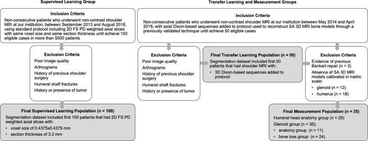
This retrospective study received institutional review board approval, under Health Insurance Portability and Accountability Act waiver of consent. There were three patient datasets involved in this study, nonconsecutive, collected through an electronic database search using keywords and examination codes (Fig 1): (a) One hundred patients (average age, 44 years; range, 14–80 years; 60 men) were included in the supervised learning group, (b) 50 patients (average age, 33 years; range, 16–65 years; 35 men) in the transfer learning group, and (c) 35 patients (average age, 33 years; range, 19–64 years; 23 men) in the measurement group.

Figure 1:

Flowchart illustrates inclusion and exclusion criteria and final study population enrolled in each part of the project. FA = fully automated segmented, FS PD = fat-suppressed proton-density, SA = semiautomated segmented, 3D = three-dimensional, 2D = two-dimensional.

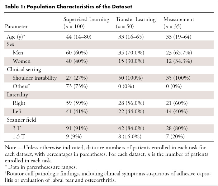
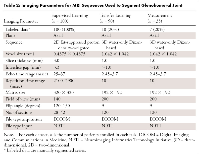
The inclusion criterion for the supervised learning group was undergoing noncontrast shoulder MRI performed between September 2013 to August 2018. For the transfer learning and measurement groups, the inclusion criterion was undergoing shoulder MRI including Dixon-based sequences performed between May 2014 and April 2019. Our dataset covered a range of common shoulder pathologic conditions, including rotator cuff and/or tendinopathy, labral tears, shoulder instability, adhesive capsulitis, and osteoarthritis. Our exclusion criteria included poor image quality, previous shoulder surgery, humeral shaft fractures, and history and/or presence of tumor. The population and the imaging characteristics of the dataset are summarized in Tables 1 and 2 (Appendix E1 [supplement]).

Table 1:

Population Characteristics of the Dataset

Table 2:

Imaging Parameters for MRI Sequences Used to Segment Glenohumeral Joint

Segmentation Model

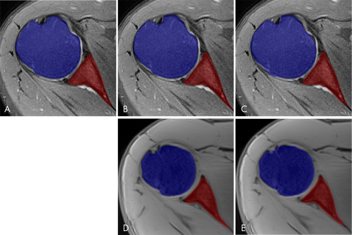
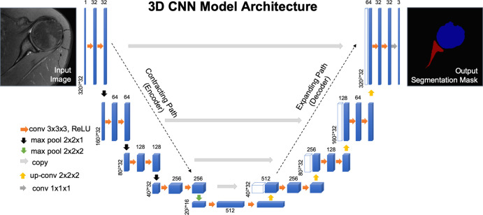
Each imaging series was manually segmented by a musculoskeletal radiologist (T.C.R., 4 years of experience) using open-source software (ITK-SNAP v3.6.0; www.itksnap.org) (10) (Fig 2, A). Both 2D and 3D CNNs based on U-Net architecture (Fig 3) (11) were used to develop a fully automated bone segmentation model for proton density–weighted images. For the 2D and 3D CNNs, 2D slices and 3D volume, respectively, and corresponding segmentation mask were used as a single training sample. Models were trained using the weighted cross-entropy loss function to overcome the imbalanced segmentation class problem. An adaptive moment estimation optimizer was used with a learning rate of 1×10⁻⁵ and batch size of 16 for the 2D CNN and one for the 3D CNN. TensorFlow software library (v1.10.0; https://www.tensorflow.org) was used to implement CNNs (Appendix E1 [supplement]).

Figure 2:

Comparison between different segmentation masks of glenohumeral joint bones. Multiple segmentation masks of the same patient where blue represents humeral head and red represents glenoid. A, Manual segmentation mask performed by a musculoskeletal radiologist using free open-source software (ITK-SNAP), overlapping an axial fat-suppressed proton density–weighted slice of shoulder, which was used as ground truth for training and to evaluate the deep learning model and fully automated segmentation masks generated by a trained deep learning algorithm using B, two-dimensional (2D) convolutional neural network (CNN) and C, three-dimensional (3D) CNN U-Net–based architecture through supervised learning of an axial 2D fat-suppressed proton density–weighted MRI dataset. D, 2D CNN and E, 3D CNN U-Net–based architectures generated fully automated segmentation masks for a different patient through transfer learning of a 3D water-only Dixon-based dataset performed by a deep learning algorithm.

Figure 3:

U-shaped architecture of the three-dimensional convolutional neural network (3D CNN) model used for supervised learning. Algorithm model where blue rectangles represent feature maps with the size and the number of feature maps indicated. White boxes represent copied feature maps. The number of feature maps doubles at each pooling. The architecture represented in this model contains 64 feature maps in the first and last layer of the network and four layers in the contracting and expanding path. The purpose of the contracting path is to capture the context of the input image to be able to do segmentation. The purpose of the expanding path is to enable precise localization combined with contextual information from the contracting path. The color-coded arrows denote different operations in this neural network. Max pool = max-pooling layer, ReLU = rectified linear unit.

Fourfold cross-validation was performed during training. Training was performed using an early stopping criterion to prevent overfitting and stopped when the accuracy on the validation set did not improve by 10⁻⁸ within the last 20 epochs. An optimal threshold for each cross-validation model and bones was identified using precision-recall curve analysis on the validation set by choosing the point on the precision-recall curve that had the smallest Euclidean distance to the maximum precision and recall (12). Then each 2D slice and 3D volume was processed in the trained 2D or 3D CNN to obtain the corresponding 2D or 3D segmentation mask using the threshold (Fig 2, B and C). For 2D CNN, the 3D segmentation mask was generated by stacking 2D segmentation masks in the slice order. Using 3D segmentation mask connectivity analysis, we identified the segmentation labels for each voxel that corresponded to the maximum connected volume for each bone.

Transfer Learning

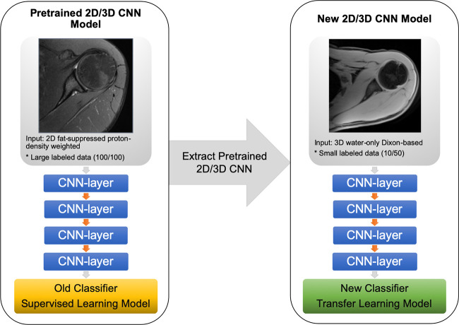
We transferred the representation learned from the proton-density images to the water-only Dixon-based sequences (Fig 4). The models developed for the proton-density images were used as a baseline model for training using a fourfold cross-validation. All the layers of baseline CNN models were retrained during transfer learning using a weighted cross-entropy loss and an adaptive moment estimation optimizer with a learning rate of 1×10⁻⁵ and batch size of 16 for the 2D CNN and one for the 3D CNN. Training was performed using an early stopping criterion to prevent overfitting and stopped when the accuracy on the validation set did not improve by 10⁻⁸ within the last 20 epochs (Appendix E1 [supplement]). Using the four transfer-learned models from fourfold cross-validation, bone segmentation masks were identified using an average probability map obtained from these models and thresholding it by 0.5 for 2D CNN. For 3D CNN, four interleaved 3D volumes of 32 slices each were processed and combined using four transfer-learned models. Thresholding the average bone probabilities from four models was used to generate segmentation masks (Fig 2, D and E).

Figure 4:

Diagram of the convolutional neural network (CNN) transfer learning models. The two- and three-dimensional (2D and 3D) CNN model used in this study was pretrained through supervised learning on axial 2D fat-suppressed proton density–weighted slices from shoulder MRI to obtain a segmentation mask classifier (yellow rectangle) using a dataset (100 total, 100 labeled). Parameters were extracted from the pretrained model and applied through transfer learning to another dataset (50 total, 10 labeled) of axial 3D water-only Dixon-based sequence slices of shoulder MRI to obtain a new segmentation mask classifier (green rectangle).

3D Model Production and Measurements

We postprocessed the fully automated segmentation masks using a medical open-source software (3DSlicer v4.11.0; www.slicer.org) to create 3D volume surface-rendered models through the volume intensity (Fig 5) (Appendix E1 [supplement]). Semiautomated 3D models, created using a previously validated method (1,4), were used as the reference standard for normal anatomy and GBL measurements.

Figure 5:

Three-dimensional (3D) MRI bone models, fully automated segmentation by 3D convolutional neural network for 3D water-only Dixon-based sequence postprocessed with 3D volume surface mask. A, 3D MRI bone model of glenohumeral joint created by the selection of a threshold range of 1.00 to 3.00 of volume intensity from a 28-year-old man with previous history of anterior shoulder instability. B, “En face” view of the 3D MRI glenoid model obtained with a range of 1.00 to 1.01 volume intensity shows no clinically significant glenoid bone loss and C, shows a Hill-Sachs lesion (dashed line) at the 3D MRI humeral head model obtained with a range of 2.99 to 3.00 of volume intensity.

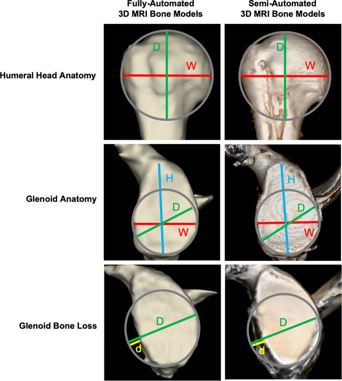
There were two separate measurement sessions using both the fully automated and semiautomated 3D models. At the first session, two musculoskeletal radiologists (E.F.A., T.C.R.; 4 years of experience each) independently, and blind to prior clinical and imaging reports, performed anatomic and GBL percentage measurements on the 3D models. Two weeks after the first session, reader 1 repeated all measurements during a second session to evaluate intrareader agreement (Fig 6) (Appendix E1 [supplement]).

Figure 6:

Comparison between the segmented fully automated and semiautomated three-dimensional (3D) MRI models. The following measurements, in millimeters, were performed on the different 3D models: red lines for width (W), blue lines for height (H), green lines for diameter (D), and yellow lines for the size of glenoid bone loss (d) using the best-fit circle method. In each row of the figure, there is a comparison between a fully automated 3D model and semiautomated 3D model for the same patient, with the first column consisting of fully automated 3D models generated by the deep learning–based method and the second column containing the semiautomated 3D models.

We also evaluated how often a difference in GBL percentage measurement on the fully automated 3D models, compared with the semiautomated 3D models, would potentially impact patient treatment selection based on clinical practice at our institution: Patients with equal to or less than 20% would typically undergo Bankart repair, while patients with greater than 20% would typically undergo bone augmentation surgery (9).

Statistical Analysis

The area under the precision-recall curve (average precision) analysis of modeled CNNs on the dataset was used as a measure of a classifier’s performance for comparing different CNNs. Manual segmentations were used to evaluate the performance of the 2D and 3D CNNs through Dice similarity coefficient (DSC), sensitivity, precision, and surface-based distance measurements (13). We defined as outliers any segmentations in which the individual DSC was below 0.8. The outliers were analyzed individually to identify causal factors.

The 3D MRI model measurements were compared using matched-pairs Wilcoxon signed rank test. All statistical tests were conducted at the two-sided 5% significance level using SAS 9.4 software (SAS Institute, Cary, NC) (Appendix E1 [supplement]).

Results

Overview of 2D and 3D CNN Segmentation Models

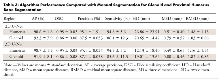
Evaluating the 100 cases in the segmentation group, the 2D CNN segmentation of the humerus achieved a DSC of 0.95, precision of 95.1%, average precision of 98.6%, and sensitivity of 94.8%. For the glenoid, there was a DSC of 0.86, precision of 87.5%, average precision of 92.3%, and sensitivity of 86.1%. The surface-based distance measurements are summarized in Table 3. We had eight outliers for the 2D CNN. They presented false-negative voxels in areas with bone marrow edema, bone marrow heterogeneity, and image artifacts (ie, motion and field inhomogeneity) (Appendix E1, Table E1 [supplement]).

Table 3:

Algorithm Performance Compared with Manual Segmentation for Glenoid and Proximal Humerus Bone Segmentation

The 3D CNN segmentation of the humerus achieved a DSC of 0.95, precision of 95.1%, average precision of 98.7%, and sensitivity of 94.9%. For the glenoid, there was a DSC of 0.86, precision of 87.1%, average precision of 91.9%, and sensitivity of 85.6%. The surface-based distance measurements are summarized in Table 3. For the 3D CNN, we had nine outliers. They presented false-negative voxels in areas with bone marrow heterogeneity, bone marrow edema, and image artifacts. They also presented partial volume effect causing false-negative and false-positive voxels, and false-positive voxels in areas of subcutaneous fat (Appendix E1, Table E1 [supplement]).

A musculoskeletal radiologist performed a visual review of the created 3D models using a 3D CNN. Patients without semiautomatic models calibrated in metric scale were excluded (12 glenoids, 18 humeri). Three patients were excluded due to evidence of previous surgery. All of the segmentation masks created by the 3D CNN were selected, as all of the 3D models were found satisfactory during the visual review. Measurements were performed on a total of 35 glenoid and 29 humerus models. The glenoid patients were divided into two groups: 11 patients without GBL to evaluate normal anatomy and 24 patients with GBL.

Humeral Head Anatomy

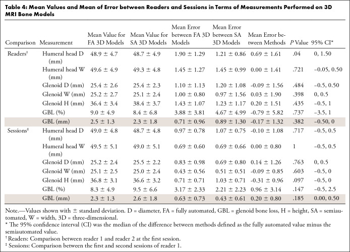
The mean humeral head diameter on the fully automated 3D models was 48.9 mm (range, 39–57 mm), while the mean width was 49.6 mm (range, 39–57 mm) for both readers at the first session. On the semiautomated 3D models, the mean diameter was 48.7 mm (range, 39–57 mm), while the mean width was 49.3 mm (range, 39–57 mm). There were no differences found when comparing the humeral head width measurements (P = .721). The mean error between humeral head diameter measurements was 0.69 mm (P = .040). The 95% confidence intervals for the difference between the fully and semiautomated models, in terms of the mean error between the diameter and width measurements between the two readers, were between 0.0% and 1.50% and −0.50% and 0.50%, respectively. The mean of the error between readers and sessions is summarized in Table 4.

Table 4:

Mean Values and Mean of Error between Readers and Sessions in Terms of Measurements Performed on 3D MRI Bone Models

Glenoid Anatomy

The mean glenoid diameter on the fully automated 3D models was 25.4 mm (range, 21–29 mm), mean width was 25.2 mm (range, 21–29 mm), and mean height was 36.4 mm (range, 32–42 mm) for both readers at the first session. On the semiautomated 3D models, the mean glenoid diameter was 25.4 mm (range, 21–29 mm), mean width was 25.1 mm (range, 20–29 mm), and mean height was 36.4 mm (range, 32–42 mm). There were no differences found when comparing the glenoid measurements (P value range, .097–.763). The 95% confidence intervals for the difference between the fully and semiautomated models in terms of the mean errors between diameter measurements, width measurements, and height measurements between the two readers were between −0.50% and 0.50%, 0% and 0.50%, and −0.50% and 1.00%, respectively. The mean of the error between readers and sessions is summarized in Table 4.

GBL Results

The mean GBL size on the fully automated 3D models was 2.5 mm (range, 0–5 mm), while the mean percentage was 9.0% (range, 0%–22%) for both readers at the first session. On the semiautomated 3D models, the mean GBL size was 2.3 mm (range, 0–6 mm), while the mean percentage was 8.4% (range, 0%–24%). There was no difference found when comparing the GBL percentage (P value range, .147–.737). The 95% confidence intervals for the difference between the fully and semiautomated models in terms of the mean error between the GBL percentage between the two readers and by the same reader in different sessions were −3.50% and 1.00% and −0.50% and 2.50%, respectively. The mean of the error between readers and sessions is summarized in Table 4.

Treatment Impact

We evaluated how often a difference in the GBL measurement generated by the fully automated model compared with the semiautomated model (reference standard) would impact treatment selection. We found that differences in GBL measurement would have impacted one of 24 patients for each reader during the first session and two of 24 patients for reader 1 during the second session. In all disagreements, the reader underestimated the amount of GBL, which would have indicated a Bankart repair instead of bone augmentation (Appendix E1 [supplement]).

Discussion

We demonstrated the feasibility of a time‐efficient, fully automated MRI segmentation method for the glenohumeral joint based on CNNs, with high accuracy (for both 2D and 3D CNNs, DSC of glenoid was 0.86 ± 0.08, P = .84; and DSC of humerus was 0.95 ± 0.03, P = .64) and an average segmentation time on the order of seconds. We were able to use this method to create accurate 3D MRI models of the glenohumeral joint and produce reliable quantifications of GBL. The accuracy of 3D MRI models for the evaluation of glenohumeral anatomy and GBL has been established (1,4).

Our study found no differences in terms of humeral head and glenoid anatomy when comparing fully automated 3D models to models produced using a previously validated semiautomated technique (P value range, .040–.99) (1,4). There was also no difference when comparing the GBL percentage estimated on the two sets of 3D models (P value range, .147–.737).

We chose to use the validation set to select the optimal threshold and to decide on an early stopping epoch number. Threshold selected by validation set resulted in similar DSC; however, when comparing 2D CNN with 3D CNN performance for transfer learning and considering the number of satisfactory 3D bone models, the 3D CNN was superior. Our results obtained with supervised learning compared favorably to a similar study on segmentation of the humerus and scapula using reinforcement learning by He et al (DSC of humerus, 0.923; scapula, 0.753) (14). The lower values for the glenoid and scapula segmentations in comparison with the humeral segmentations in both studies are likely related to the complex anatomy and morphologic variability of the glenoid and scapula (15,16).

Deep learning models have achieved relatively good results in a variety of applications (17), including musculoskeletal imaging (6,7,12,18–21). CNNs have gained great interest in medical image analysis as they result in the extraction of important information around a particular pixel or voxel, making it useful for common tasks like segmentation (17). A U-Net architecture was selected for our study as it has been shown to provide promising segmentation of medical imaging (6–8), particularly for bone segmentations using MRI (12). Our model accuracy was similar to long bone segmentation findings from recent studies that used a U-Net–shaped model algorithm for the femur (DSC range, 0.89–0.95) (12) and for the knee (residual mean square distance range, 2.01–2.20 mm) (6).

We used transfer learning parameters from a CNN pretrained on proton density images instead of training from scratch with new Dixon-based imaging datasets. This allowed us to train with a smaller dataset and reduced the amount of time that would typically be spent performing manual segmentations. Transfer learning has been used in medical image classification based on CNNs extensively, and it has been shown to improve generalization for the task where a limited number of samples exists (22).

Automated analysis of MRI is challenging, with various factors contributing to the difficulty of segmenting musculoskeletal structures, including varying image contrast, partial volume effects, inherent heterogeneity of image intensity, and image artifacts (6). Deep learning techniques improve with more data in a continuous learning process. Future work entailing the continuous addition of more patients would provide a larger, more variable dataset, which could help reduce the amount of errors at the segmentation masks and increase the likelihood of producing suitable 3D MRI models.

We also looked to see if a difference in a GBL estimate on models would impact patient clinical care based on a commonly accepted threshold of GBL (9). Using the fully automated 3D models, changes in the type of treatment indicated would have been rare based on our readers’ measurements. It is understood that there are a number of factors that impact treatment selection for patients with anterior shoulder instability. Our analysis was a hypothetical simplified algorithm that focused on the impact that GBL imaging characterization can have on treatment selection to further investigate the fully automated 3D models.

Our study had several limitations. While our dataset covered a range of common shoulder abnormalities, including shoulder instability, rotator cuff pathologic conditions, labral tears, adhesive capsulitis, and osteoarthritis, some pathologic conditions, including tumors and proximal humeral shaft fractures, and patients with prior surgery were excluded from our datasets during the training phase. Image segmentation is a fast-growing field with new training approaches for losses presented each year. Comparing our results using different loss functions (23) instead of weighted cross-entropy is beyond the scope of this work. Internal validation of our deep learning model may not be sufficient or indicative for its performance in future patients. We did not perform external validation of our CNN model, which is essential before implementing prediction models in clinical practice. Other limitations included a small sample size to evaluate the accuracy of fully automated 3D models.

Our fully automated segmentation method serves as a first step toward providing rapid and accurate 3D MRI glenohumeral bone models that can be potentially used in clinical practice. Such a model would improve our daily workflow by decreasing the likelihood of delayed imaging reports related to imaging postprocessing for this patient population. Last, CNNs could be used to produce 3D MRI bone models with smaller datasets though the use of transfer learning methods.

References

- 1.Gyftopoulos S, Yemin A, Mulholland T, et al. 3DMR osseous reconstructions of the shoulder using a gradient-echo based two-point Dixon reconstruction: a feasibility study. Skeletal Radiol 2013;42(3):347–352. [DOI] [PubMed] [Google Scholar]
- 2.Rerko MA, Pan X, Donaldson C, Jones GL, Bishop JY. Comparison of various imaging techniques to quantify glenoid bone loss in shoulder instability. J Shoulder Elbow Surg 2013;22(4):528–534. [DOI] [PubMed] [Google Scholar]
- 3.Bishop JY, Jones GL, Rerko MA, Donaldson C, MOON Shoulder Group . 3-D CT is the most reliable imaging modality when quantifying glenoid bone loss. Clin Orthop Relat Res 2013;471(4):1251–1256. [DOI] [PMC free article] [PubMed] [Google Scholar]
- 4.Gyftopoulos S, Beltran LS, Yemin A, et al. Use of 3D MR reconstructions in the evaluation of glenoid bone loss: a clinical study. Skeletal Radiol 2014;43(2):213–218. [DOI] [PubMed] [Google Scholar]
- 5.Samim M, Eftekhary N, Vigdorchik JM, et al. 3D-MRI versus 3D-CT in the evaluation of osseous anatomy in femoroacetabular impingement using Dixon 3D FLASH sequence. Skeletal Radiol 2019;48(3):429–436. [DOI] [PubMed] [Google Scholar]
- 6.Liu F, Zhou Z, Jang H, Samsonov A, Zhao G, Kijowski R. Deep convolutional neural network and 3D deformable approach for tissue segmentation in musculoskeletal magnetic resonance imaging. Magn Reson Med 2018;79(4):2379–2391. [DOI] [PMC free article] [PubMed] [Google Scholar]
- 7.Zhou Z, Zhao G, Kijowski R, Liu F. Deep convolutional neural network for segmentation of knee joint anatomy. Magn Reson Med 2018;80(6):2759–2770. [DOI] [PMC free article] [PubMed] [Google Scholar]
- 8.Liu F, Zhou Z, Samsonov A, et al. Deep Learning Approach for Evaluating Knee MR Images: Achieving High Diagnostic Performance for Cartilage Lesion Detection. Radiology 2018;289(1):160–169. [DOI] [PMC free article] [PubMed] [Google Scholar]
- 9.Di Giacomo G, de Gasperis N, Scarso P. Bipolar bone defect in the shoulder anterior dislocation. Knee Surg Sports Traumatol Arthrosc 2016;24(2):479–488. [DOI] [PubMed] [Google Scholar]
- 10.Yushkevich PA, Piven J, Hazlett HC, et al. User-guided 3D active contour segmentation of anatomical structures: significantly improved efficiency and reliability. Neuroimage 2006;31(3):1116–1128. [DOI] [PubMed] [Google Scholar]
- 11.Ronneberger O, Fischer P, Brox T. U-Net: Convolutional Networks for Biomedical Image Segmentation. CoRR: arXiv:1505.04597. [preprint] https://arxiv.org/abs/1505.04597. Posted 2015. Accessed April 2020.
- 12.Deniz CM, Xiang S, Hallyburton RS, et al. Segmentation of the Proximal Femur from MR Images using Deep Convolutional Neural Networks. Sci Rep 2018;8(1):16485. [DOI] [PMC free article] [PubMed] [Google Scholar]
- 13.Taha AA, Hanbury A. Metrics for evaluating 3D medical image segmentation: analysis, selection, and tool. BMC Med Imaging 2015;15(1):29. [DOI] [PMC free article] [PubMed] [Google Scholar]
- 14.He X, Tan C, Qiao Y, Tan V, Metaxas D, Li K. Effective 3D Humerus and Scapula Extraction using Low-contrast and High-shape-variability MR Data. eprint arXiv:1902.08527. [preprint] https://arxiv.org/abs/1902.08527. Posted 2019. Accessed June 2020. [Google Scholar]
- 15.Gray DJ. Variations in human scapulae. Am J Phys Anthropol 1942;29(1):57–72. [Google Scholar]
- 16.Strauss EJ, Roche C, Flurin PH, Wright T, Zuckerman JD. The glenoid in shoulder arthroplasty. J Shoulder Elbow Surg 2009;18(5):819–833. [DOI] [PubMed] [Google Scholar]
- 17.Shen D, Wu G, Suk HI. Deep Learning in Medical Image Analysis. Annu Rev Biomed Eng 2017;19(1):221–248. [DOI] [PMC free article] [PubMed] [Google Scholar]
- 18.Lee JG, Gumus S, Moon CH, Kwoh CK, Bae KT. Fully automated segmentation of cartilage from the MR images of knee using a multi-atlas and local structural analysis method. Med Phys 2014;41(9):092303. [DOI] [PMC free article] [PubMed] [Google Scholar]
- 19.Norman B, Pedoia V, Majumdar S. Use of 2D U-Net Convolutional Neural Networks for Automated Cartilage and Meniscus Segmentation of Knee MR Imaging Data to Determine Relaxometry and Morphometry. Radiology 2018;288(1):177–185. [DOI] [PMC free article] [PubMed] [Google Scholar]
- 20.Prasoon A, Petersen K, Igel C, Lauze F, Dam E, Nielsen M. Deep feature learning for knee cartilage segmentation using a triplanar convolutional neural network. Med Image Comput Comput Assist Interv 2013;16(Pt 2):246–253. [DOI] [PubMed] [Google Scholar]
- 21.Zeng G, Zheng G. Deep Learning-Based Automatic Segmentation of the Proximal Femur from MR Images. Adv Exp Med Biol 2018;1093:73–79. [DOI] [PubMed] [Google Scholar]
- 22.Litjens G, Kooi T, Bejnordi BE, et al. A survey on deep learning in medical image analysis. Med Image Anal 2017;42:60–88. [DOI] [PubMed] [Google Scholar]
- 23.Taghanaki SA, Abhishek K, Cohen JP, Cohen-Adad J, Hamarneh G. Deep Semantic Segmentation of Natural and Medical Images: A Review. arXiv:1910.07655. [preprint] https://arxiv.org/abs/1910.07655. Posted 2019. Accessed April 2020. [Google Scholar]
Associated Data
This section collects any data citations, data availability statements, or supplementary materials included in this article.