

Summary
We propose sensitivity analyses for publication bias in meta‐analyses. We consider a publication process such that ‘statistically significant’ results are more likely to be published than negative or “non‐significant” results by an unknown ratio, η. Our proposed methods also accommodate some plausible forms of selection based on a study's standard error. Using inverse probability weighting and robust estimation that accommodates non‐normal population effects, small meta‐analyses, and clustering, we develop sensitivity analyses that enable statements such as ‘For publication bias to shift the observed point estimate to the null, “significant” results would need to be at least 30 fold more likely to be published than negative or “non‐significant” results’. Comparable statements can be made regarding shifting to a chosen non‐null value or shifting the confidence interval. To aid interpretation, we describe empirical benchmarks for plausible values of η across disciplines. We show that a worst‐case meta‐analytic point estimate for maximal publication bias under the selection model can be obtained simply by conducting a standard meta‐analysis of only the negative and ‘non‐significant’ studies; this method sometimes indicates that no amount of such publication bias could ‘explain away’ the results. We illustrate the proposed methods by using real meta‐analyses and provide an R package: PublicationBias.
Keywords: File drawer, Meta‐analysis, Publication bias, Sensitivity analysis
1. Introduction
Publication bias can distort meta‐analytic results, sometimes justifying considerable scepticism towards meta‐analyses reporting positive findings. Numerous statistical methods, mostly falling into two broad categories, help to assess or correct for these biases. First, classical methods arising from the funnel plot (Duval and Tweedie, 2000; Egger et al., 1997) assess whether small studies have systematically larger point estimates than larger studies (see Jin et al. (2015) for a review). These methods effectively assume that publication bias does not operate on very large studies and operates on the basis of the size of the point estimates rather than their p‐values. A second class of methods, called selection models, instead assumes that publication bias selects for small p‐values rather than large point estimates and allows for publication bias that operates on all studies, not only on small studies (see Jin et al. (2015) and McShane et al. (2016) for reviews). These models specify a parametric form for the population effect distribution as well as for the dependence of a study's publication probability on its p‐value. The latter weight function may, for example, be specified as a step function such that ‘affirmative’ results (i.e. positive point estimates with a two‐tailed p<0.05) are published with higher probability than ‘non‐affirmative’ results (i.e. negative point estimates or those with p⩾0.05) (e.g. Dear and Begg (1992), Hedges (1992) and Vevea and Hedges (1995)). Then, after weighting each study's contribution to the likelihood by its inverse probability of publication per the weight function, the meta‐analytic parameters of interest and the parameters of the weight function can be jointly estimated by maximum likelihood. Some relatively recent methods can be viewed as hybrids between classical funnel plot methods and selection models (Bom and Rachinger, 2019; Stanley and Doucouliagos, 2014).
Existing selection models focus on thus estimating bias‐corrected meta‐analytic estimates as well as the severity of publication bias itself. These models, although quite valuable and informative for large meta‐analyses, often yield unstable estimates in meta‐analyses of typical sizes (Field and Gillett, 2010; Vevea and Woods, 2005), particularly when the number of upweighted studies (e.g. affirmative studies as defined above) is also small. In practice, most meta‐analyses are far too small to apply selection models; for example, the percentage of meta‐analyses comprising fewer than 10 studies probably exceeds 50% in the Cochrane database (Ioannidis and Trikalinos, 2007) and in medical journals (Sterne et al., 2000). Selection models may in fact require considerably more than 10 studies to achieve their asymptotic properties (Field and Gillett, 2010). Vevea and Woods (2005) therefore proposed to repurpose selection models to conduct sensitivity analyses across a fixed range of parameters that govern the severity of publication bias, rather than attempting to estimate these parameters jointly. If the results of a meta‐analysis are only mildly attenuated even under severe publication bias, then the results might be considered fairly robust to publication bias (Vevea and Woods, 2005), whereas if the results are severely attenuated under mild publication bias the results might be considered sensitive to publication bias. These methods, like selection models in general, require specifying a parametric form on the population effect distribution, but related work suggests that results can be highly sensitive to this specification (Johnson et al., 2017). Empirical assessment of distributional assumptions may be particularly challenging when the distribution of point estimates is already distorted because of publication bias. Additionally, the method of Vevea and Woods (2005) seems to model the sensitivity parameters as if they were observed data: an apparent vestige of the model's original purpose of estimating these parameters rather than conducting sensitivity analysis across fixed parameters (Hedges, 1992). Therefore, when the sensitivity parameters reflect more severe publication bias than actually exists, the corrected point estimate can sometimes be overcorrected.
A different approach to sensitivity analysis considers the ‘fail‐safe number’, which is defined as the minimum number of unpublished studies with a mean point estimate of 0 (or another fixed value) that would need to exist for their inclusion in the meta‐analysis to reduce the pooled point estimate to ‘statistical non‐significance’ (Rosenthal, 1979) or to a given effect size threshold (Orwin, 1983). These methods typically assume homogeneous population effects (Schmidt and Hunter, 2014) and require specification of the mean of the unpublished studies’ point estimates.
Here, we develop sensitivity analyses that advance methodologically on these existing approaches and also enable particularly simple intuitive statements regarding sensitivity to publication bias. Methodologically, the present methods relax the distributional and asymptotic assumptions that are used in existing selection models, i.e. our methods require specification of a simple weight function but do not require any distributional assumptions on the population effects, and they accommodate dependence among the point estimates that can arise when some papers contribute multiple point estimates. Our proposed methods also provide correct inference in meta‐analyses with a realistically small total number of studies, as well as with few observed non‐affirmative studies. We shall show that, for common effect meta‐analysis (also called ‘fixed effects meta‐analysis’; Rice et al. (2018)), sensitivity analyses can be conducted in closed form and, for random‐effects meta‐analysis, they can be conducted through a numerical grid search.
Additionally, our proposed methods enable conclusions that are particularly straightforward to interpret and report: a key consideration for sensitivity analyses to gain widespread use (e.g. VanderWeele and Ding (2017) and VanderWeele et al. (2019)). That is, analogously to recent work on sensitivity analysis for unmeasured confounding (VanderWeele and Ding, 2017), the present methods allow statements such as ‘For publication bias to “explain away” the meta‐analytic pooled point estimate completely (i.e. to attenuate the population effect to the null), affirmative results would need to be at least 30 fold more likely to be published than non‐affirmative results; for publication bias to attenuate the confidence interval to include the null, affirmative results would need to be at least 16 fold more likely to be published than non‐affirmative results’. Large ratios of publication probabilities would therefore indicate that the meta‐analysis is relatively robust to publication bias, whereas small ratios would indicate that the meta‐analysis is relatively sensitive to publication bias. We discuss empirical benchmarks for plausible values of these ratios based on a systematic review of existing meta‐analyses across several empirical disciplines. We also extend these sensitivity analyses to assess the amount of publication bias that would be required to attenuate the point estimate or its confidence interval to any non‐null value, which is an approach that has been used in existing sensitivity analyses for other forms of bias (e.g. Ding and VanderWeele (2016) and VanderWeele and Ding (2017)). These sensitivity analyses apply when the publication process is assumed to favour ‘statistically significant’ and positive results over ‘non‐significant’ or negative results; the analyses also accommodate some forms of additional selection on studies’ standard errors without requiring any modifications.
This paper is structured as follows. We first describe three standard meta‐analytic specifications for which we shall develop sensitivity analyses (Section 2). We describe our assumed model of publication bias (Section 2.2) and use it to incorporate bias corrections in the three meta‐analytic specifications and thus to conduct sensitivity analyses (Section 3). We discuss how to interpret the results in practice, providing evidence‐based guidelines for plausible values of the sensitivity parameters and suggesting a simple graphical aid to interpretation (Section 6). We illustrate the methods with three applied examples (Section 7) and present a simulation study demonstrating the methods’ robustness in challenging scenarios (Section 8). Last, we discuss the plausibility of our assumed model of publication bias and describe how our proposed methods could be extended to accommodate other models (Section 9).
2. Setting and notation
2.1. Common effect and robust random‐effects meta‐analysis
Throughout, we consider a meta‐analysis of k studies, in which and respectively denote the point estimate and squared standard error of the ith meta‐analysed study. We assume the mean model , where (treated as known, as usual in meta‐analysis) and var(γ i)=τ 2. As usual in meta‐analysis, we assume that the point estimates and their standard errors are uncorrelated in the underlying population of studies before selection based on publication bias. The common effect specification, arising under the additional assumption that τ 2=0 and that the errors ε i are independent, estimates μ and its variance as the weighted average of the point estimates:
| (2.1) |
(If τ 2>0, but interest lies in drawing inference only on the sample of meta‐analysed studies rather than on a broader population from which the meta‐analysed studies were drawn, the common effect estimate and variance in fact remain unbiased with correct nominal coverage (Rice et al., 2018).) Alternatively, if τ 2 may be greater than 0 and we intend to draw inference on a broader population of studies, then μ and its variance can be estimated under a random‐effects model. For this case, we consider a robust estimation approach that is similar to generalized least squares which, unlike standard parametric random‐effects meta‐analysis, yields consistent estimates of μ without requiring the usual distributional and independence assumptions on ε i or γ i (Hedges et al., 2010). Additionally, whereas standard asymptotic inference for parametric random‐effects meta‐analysis can perform poorly for small k, simple corrections enable the robust specification to perform quite well in small samples (Tipton, 2015); this will become especially important when we consider sensitivity analyses for which the effective sample size is further reduced through inverse probability weighting.
Specifically, following Hedges et al. (2010), suppose that there are M clusters with estimates in the mth cluster. For example, each cluster might represent a paper that potentially contributes to the meta‐analysis multiple, statistically independent point estimates arising from a hierarchical structure in which different papers have different mean effect sizes due, for example, to the use of different subject populations. Alternatively, each cluster might represent a paper for which there is a single population effect size, but in which point estimates are statistically dependent because they are estimated in overlapping groups of subjects (Hedges et al., 2010). Arbitrary other correlation structures are also possible, and importantly, as in generalized estimating equations with robust inference, correct prespecification of the correlation structure allows optimal efficiency but is not required to achieve correct inference asymptotically or in finite samples with a small sample correction (Hedges et al., 2010). The usual meta‐analytic assumption of independent point estimates represents the special case with M=k, for all m, and an intercluster correlation of 0; we term this the robust independent specification.
Let be the vector of point estimates for studies in cluster m. For the general case, which we shall term the robust clustered specification, the point estimates may be arbitrarily dependent within clusters but are assumed to be independent across clusters. That is, let denote the within‐cluster covariance matrix of the study level error terms, , and let Σ= diag(Σ1,…,ΣM) denote the overall covariance matrix. Let be a diagonal matrix of arbitrary positive weights for studies in cluster m, such that the ith study in cluster m has weight w mi. Let denote the 1‐vector of length . Then, as a direct special case of equations (3) and (6) of Hedges et al. (2010), a consistent estimate of μ and its exact variance are
| (2.2) |
Letting denote the vector of residuals for studies in cluster m, an asymptotic plug‐in estimate of the variance is
| (2.3) |
(This model and the corresponding sensitivity analyses that are developed below also extend readily to meta‐regression; see Hedges et al. (2010) for details. We focus on the intercept‐only model for brevity.) In all subsequent work, we shall use Tipton's (2015) finite sample correction to this variance estimator, which can be easily applied in R by fitting the model with the robumeta package (Fisher and Tipton, 2015) with the argument small=TRUE and is also implemented in our R package PublicationBias. We next describe our assumed model of publication bias and develop sensitivity analyses for the common effect, robust independent and robust clustered specifications.
2.2. Assumed model of publication bias
We consider a mechanism of publication bias in which studies are selected for publication from among an underlying population of all published and unpublished studies, and the probability of selection is higher for affirmative (defined by and p<0.05) versus non‐affirmative studies (defined by or p⩾0.05). (Throughout, we assume that publication favours point estimates in the positive direction and that the uncorrected is positive. As described in Section 4, if publication instead favours results with negative point estimates and , we can simply reverse the sign of all point estimates and of the meta‐analytic summary statistics before conducting our proposed analyses. Alternatively, if there is a strong reason to believe that publication bias operates on the basis of an α‐level other than 0.05 for a given meta‐analysis, e.g. because of disciplinary conventions, the definition of affirmative status can simply be generalized to require and p<α with no further changes to the following results.) This model of publication bias is common in existing work (see McShane et al. (2016) for a review), and in Section 9 we discuss in detail its plausibility and extensions to other models of publication bias. Suppose that the underlying population is of size k *⩾k, with the point estimate and standard error in the ith study denoted and respectively. Let denote the p‐value of underlying study i and be an indicator for whether underlying study i is affirmative. Let denote an additional unstandardized, common effect or random‐effects inverse variance weight; for example, for common effect meta‐analysis, . Let be an indicator for whether study i is in fact published. Then, we assume that the publication process arises as
| (2.4) |
| (2.5) |
| (2.6) |
i.e. we assume that the publication probability is η times higher for affirmative studies than for non‐affirmative studies, where we shall treat η as an unknown sensitivity parameter. The subsequent assumptions regarding uncorrelatedness state that, conditionally on a study's affirmative or non‐affirmative status, publication bias does not select further based on the inverse variance weights nor on the product of the point estimates with their inverse variance weights. For example, this assumption excludes the possibility that the publication process would favour studies with larger point estimates, smaller standard errors or smaller p‐values beyond its favouring of affirmative results. However, in the on‐line supplement (section 1.1), we show that these assumptions can in fact be relaxed to accommodate a publication process that additionally favours studies with smaller standard errors (for example) as long as this form of selection operates in the same way for affirmative and for non‐affirmative studies. As we show in the supplement, this additional form of selection can simply be ignored, requiring no modification to the sensitivity analyses that we present below.
Additionally, this model is agnostic to the reasons for preferential publication of affirmative studies, which probably reflects a complex combination of authors’ selective reporting of results (Chan et al., 2004; Coursol and Wagner, 1986) and selective submission of papers (Franco et al., 2014; Greenwald, 1975), as well as editors’ and reviewers’ biases (although some empirical work suggests that the latter may be a weaker influence than author decision making; see Lee et al. (2006) and Olson et al. (2002)). That is, we technically conceptualize the population as the population of all conducted hypothesis tests that would, if published, be included in the meta‐analysis. For example, suppose that various researchers conduct and publish 10 studies on the topic of the meta‐analysis, each involving two separate experiments on independent samples (all of which would be included in the meta‐analysis if published). If each paper includes or omits the results of these two experiments on the basis of the selection process that is defined by equations (2.4), (2.5), (2.6), the underlying population would comprise the 20 total hypothesis tests. For brevity, though, we refer to an underlying population of ‘studies’ and the aggregation of all selection effects conforming to the assumptions in equations (2.4), (2.5), (2.6) as ‘publication bias’.
Last, note that our definition of assumes that the publication process preferentially selects studies with point estimates that are both statistically significant and positive in direction. Studies with non‐significant point estimates and those with statistically significant negative point estimates are equally disfavoured. As in the existing literature (Vevea and Hedges, 1995), we refer to this as ‘one‐tailed selection’ in contrast with an alternative ‘two‐tailed selection’ model in which publication favours all studies with significant point estimates, regardless of direction. Note that the term ‘one tailed’ does not imply that studies report one‐tailed hypothesis tests, but rather that publication selects in a one‐tailed manner based on reported statistical results.
3. Main results
3.1. Sensitivity analysis under the common effect specification
3.1.1. Publication bias required to attenuate the point estimate or its lower confidence interval limit to a chosen value
Under publication bias as described above, the naive common effect estimate will usually be biased for μ if η>1. In this section, we first present consistent estimators and under a fixed ratio η, which we then use to derive sensitivity analyses characterizing the value of η that is required to attenuate or its lower confidence limit, , to a chosen smaller value q. When referring to the published and meta‐analysed, rather than underlying, studies, we use notation as in Section 2.2 above but without the asterisk superscript. For example, is an indicator for whether observed study i is affirmative. Let and respectively be the sets of published, meta‐analysed affirmative and non‐affirmative studies. For an arbitrary subset of studies , define and , such that is the usual common effect estimate for the studies in . Then, for a fixed η, consistent estimates of μ and its variance can be obtained under mild regularity conditions by weighting each study inversely to its publication probability (on‐line supplement, section 1.1, theorem 1.1):
| (3.1a) |
| (3.1b) |
Because η is not known in practice, we develop these estimators only as means to the end of deriving sensitivity analyses as follows. For a meta‐analytic effect estimate t (either or ), define S(t,q) as the value of η that would attenuate t to q, where q<t. For example, is the value of η that would attenuate the point estimate to , and its derivation for common effect meta‐analysis follows directly from equation (3.1a):
If, as usual, the point estimates are meta‐analysed on a scale for which the null is 0, then, for the special case of attenuating the point estimate to the null, we have . That is, to attenuate the point estimate to the null, affirmative studies would need to be more likely to be published than non‐affirmative studies by the same ratio by which the magnitude of exceeds its counterpart in the non‐affirmative studies, . For example, if is fivefold larger and in the opposite direction from , then to attenuate to the null, affirmative studies would need to be more likely to be published than non‐affirmative studies by fivefold.
To consider the severity of publication bias that is required to attenuate the lower 95% confidence limit of to q, we set q equal to the corrected confidence limit estimate by using the variance estimate in equation (3.1b). Letting c crit denote the two‐sided critical value for the t‐distribution on k−1 degrees of freedom, we thus have
where . When q=0, this simplifies to
In general, it is possible to obtain S(t,q)<1, which means that no amount of publication bias under the model that was described above, no matter how severe, could attenuate t to q. Additionally, S(t,q) can be reparameterized to provide an alternative metric in terms of the number of unpublished non‐affirmative studies. Specifically, S(t,q) can provide an approximate lower bound on a form of ‘fail‐safe number’, here defined as the number of unpublished non‐affirmative results that would be required to shift the statistic t to q (see the on‐line supplement, section 1.3).
3.1.2. Simple estimates under worst‐case publication bias
In addition to solving for the value of η that is required to attenuate and to specific values, it is also straightforward to estimate and for worst‐case publication bias under the model that we have assumed, i.e., letting η→∞ in equations (3.1a) and (3.1b), we have
Chemical Formula:
Since these expressions coincide with the usual common effect estimates within only the non‐affirmative studies (see equation (2.1)), worst‐case estimates under the model assumed can be obtained simply by meta‐analysing only the non‐affirmative studies. Of course, the presence of at least one non‐affirmative study in the meta‐analysis implies that η<∞ in practice, but these estimates may nevertheless serve as useful heuristics to approximate the effect of extreme publication bias.
3.2. Sensitivity under the robust random‐effects specifications
3.2.1. Publication bias required to attenuate the point estimate or its lower confidence interval limit to a chosen value
We first consider the robust clustered specification and then describe the robust independent specification as a special case. As in Section 2, suppose that there are M known clusters of point estimates. For the ith study in the mth cluster, assign the weight , so that the cluster m weight matrix is diagonal with entries equal to the product of the usual random‐effects inverse variance weights with the inverse probabilities of publication for each study. For defining these weights, we recommend simply obtaining a naive parametric estimate of in an initial meta‐analysis under the standard parametric random‐effects specification (e.g. Brockwell and Gordon (2001)) without correction for publication bias. Although this estimate may be biased due to publication bias, extreme clustering or non‐normality, this bias does not compromise point estimation or inference on μ, but rather it may only somewhat reduce efficiency because the robust specification provides unbiased estimation and valid inference regardless of the choice of W (Hedges et al., 2010). (To explore whether improving the initial estimate could improve efficiency in practice, we derived a parametric weighted score approach to estimate and a bias‐corrected jointly under independence. We assessed whether using this improved in the weights would improve performance of the robust specification (on‐line supplement, section 1.4). However, the resulting was quite biased except in very large samples, so its use did not noticeably affect efficiency. We therefore recommend simply using a naive ‐estimate.)
Then, from equations (2.2) and (2.3), we can consistently estimate μ and var(μ) for the robust clustered specification as (on‐line supplement, section 1.1, theorem 1.1):
| (3.2a) |
| (3.2b) |
(Recall that we have assumed that is chosen to be diagonal, so the double summation over clusters and individual studies in equation (2.2) reduces to a single summation over individual studies in equation (3.2a), and similarly for equations (2.3) and (3.2b). Potential correlation of estimates within clusters is accommodated through the non‐diagonal sandwich matrix in equation (3.2b).) For the robust independent specification, is identical, and simplifies to
| (3.3) |
As described in Section 2, these are asymptotic variance estimates, and in practice we recommend using Tipton's (2015) small sample correction. To approximate or , we can simply evaluate and over a grid of values of η, e.g. by passing user‐specified weights to the existing R package robumeta (Fisher and Tipton, 2015). Then, S(t,q) can be set to the smallest value of η such that t⩽q. Our R package PublicationBias automates this approach, and we illustrate further in the applied examples of Section 7.
As an alternative to the robust independent specification, it would be possible to conduct maximum likelihood sensitivity analyses under the standard parametric random‐effects model, invoking the additional assumptions that, among the published studies, γ i∼IID N(0,τ 2) and (e.g. Brockwell and Gordon (2001) and Viechtbauer (2005)). We considered this approach because it should, in principle, be more efficient than the robust specification, and it would also enable direct estimation of τ 2. In the on‐line supplement (section 1.4), we derive a parametric specification that is directly analogous to inverse probability weighting for survey sampling or missing data for general M‐estimators (Wooldridge, 2007). However, simulation results indicated that this model performed fairly poorly for moderate and large values of η (supplement, section 1.4).
3.2.2. Simple estimates under worst‐case publication bias
As seen for the common effect specification, corrected estimates for worst‐case publication bias under our assumed model can be obtained by conducting a standard, uncorrected meta‐analysis of only the non‐affirmative studies. For the robust clustered specification, letting η→∞ in equations (3.2a) and (3.2b) yields
Chemical Formula:
where denotes the set of non‐affirmative studies in cluster m, denotes the number of studies in that set and denotes a modified diagonal weight matrix for cluster m in which . Again, these expressions correspond to robustly meta‐analysing only the non‐affirmative studies (see equations (2.2) and (2.3)).
4. Additional practical considerations
4.1. Preparing data for analysis
For all three specifications above, the point estimates should be analysed on a scale such that, conditionally on their potentially non‐normal true population effects γ i, the point estimates are asymptotically approximately normal with variances . This is standard practice in meta‐analysis. For example, estimates on the hazard ratio scale can be transformed to the log‐hazard ratio scale for analysis, in which case the threshold q would also be chosen on the log‐scale. Additionally, our definition of affirmative studies assumes that estimates’ signs are coded such that positive estimates are favoured in the publication process. For meta‐analyses in which negative, rather than positive, estimates are assumed to be favoured (e.g. because negative estimates represent a protective effect of a candidate treatment), one can simply reverse the signs of the point estimates before conducting our sensitivity analyses and then reverse the sign of the bias‐corrected once more to recover the original sign convention. , with estimated after reversing signs for analysis, would be interpreted according to the original sign convention as the severity of publication bias required to shift the upper, rather than the lower, confidence interval (CI) limit to the null. For example, if the meta‐analytic estimate with the original sign convention is a hazard ratio of 0.79 (95% CI [0.71, 0.88]), and we expect publication bias to favour protective effects, we would first transform the hazard ratios to the log‐scale and reverse their signs to estimate . When interpreted according to the original sign convention and on the hazard ratio scale, would represent the severity of publication bias that is required to shift the upper CI limit of 0.88 to 1. We illustrate conducting sensitivity analyses with effect size transformations and sign reversals in the applied examples of Section 7.
4.2. Diagnostics regarding statistical assumptions
The possibility of certain violations of statistical assumptions that were described in Section 2.2 can be assessed as follows. To investigate the possibility that publication bias might favour significant results regardless of the sign of the point estimate, rather than only affirmative results, one could calculate one‐tailed p‐values for all studies and examine a histogram or density plot of these one‐tailed p‐values (e.g. using the R function PublicationBias::pval__plot). If publication bias favours significant results regardless of sign, we would expect to see an increased density of one‐tailed p‐values not only below 0.025 but also above 0.975 (because the latter corresponds to two‐tailed p‐values that are less than 0.05 with negative point estimates). To investigate whether publication bias might select on the basis of multiple α‐levels (e.g. α=0.10 as well as α=0.05), one could examine a similar density plot of two‐tailed p‐values for evidence of clear discontinuities at p‐values other than 0.05. The assumption that point estimates are not correlated with their standard errors in the underlying population is more difficult to assess because sufficiently strong publication bias that favours affirmative results will itself induce this correlation between the published studies, even if the assumption regarding the underlying population does hold. Thus, this assumption will generally need to be evaluated in terms of a priori plausibility than in terms of empirical evidence.
5. The significance funnel plot
As a visual supplement to the sensitivity analyses proposed, we suggest presenting a modified funnel plot, the ‘significance funnel’, which shares some features with other modified funnel plots, such as the contour‐enhanced funnel plot (Andrews and Kasy, 2019; Peters et al., 2008; Vevea et al., 1993). Like a standard funnel plot with or without contour enhancement, the significance funnel plot displays versus or σ i (e.g. Fig. 1(b)). Whereas a standard funnel helps to detect correlation between and σ i, the significance funnel helps to detect the extent to which the non‐affirmative studies’ point estimates are systematically smaller than the entire set of point estimates, which is the more relevant consideration when publication bias operates on statistical significance. The significance funnel distinguishes visually between affirmative studies (points to the right of the line) and non‐affirmative studies (points to the left of the line) and also displays the point estimates within all studies (the black diamond) and within only the non‐affirmative studies (the grey diamond). As discussed above, the latter represents the corrected estimate for worst‐case publication bias under the model assumed. Thus, as a simple heuristic, when the diamonds are close to one another, our quantitative sensitivity analyses will typically indicate that the meta‐analysis is fairly robust to publication bias. When the diamonds are distant or if the grey diamond represents a negligible effect size, then our sensitivity analyses may indicate that the meta‐analysis is not robust. Of course, conducting formal sensitivity analyses and reporting and for q=0 and possibly another non‐null value provides more precise information than presenting the significance funnel alone.
Figure 1.
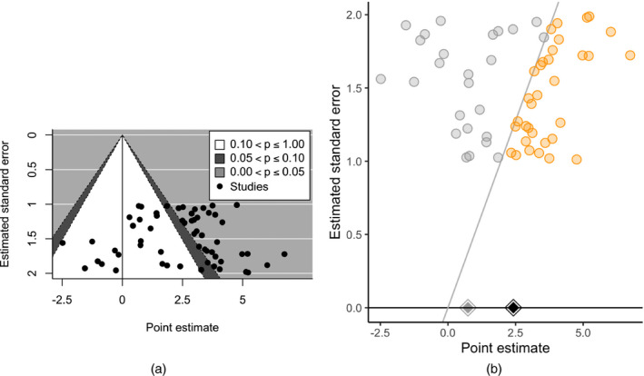
(a) Standard contour‐enhanced funnel plot (Peters et al., 2008; Viechtbauer, 2010) versus (b) significance funnel plot for data generated with publication bias and with right‐skewed population effect sizes (η=10) (studies lying on the diagonal line have exactly p=0.05):  , non‐affirmative;
  , affirmative;
  , robust independent point estimate within all studies;
  , robust independent point estimate within only the non‐affirmative studies
Even though the standard funnel and the significance funnel display the same data, the latter better complements sensitivity analyses for publication bias. Indeed, the standard funnel can be quite misleading when publication bias operates on statistical significance. For example, the standard contour‐enhanced funnel in Fig. 1(a) shows right‐skewed point estimates generated with publication bias (η=10) but suggests little correlation between the estimates and standard errors, giving an impression of robustness to publication bias under standard criteria. Yet the significance funnel (Fig. 1(b)) shows that the non‐affirmative studies in fact have much smaller point estimates than the affirmative studies, correctly suggesting that results may be sensitive to publication bias.
6. Empirical benchmarks for interpreting S(t,q)
Interpreting our proposed sensitivity analyses ultimately involves assessing whether S(t,q) is sufficiently small that it represents a plausible amount of publication bias, in which case the meta‐analysis may be considered relatively sensitive to publication bias, or conversely whether it represents an implausibly large amount of publication bias, in which case the meta‐analysis may be considered relatively robust. To help to ground such assessments empirically, we conducted a preregistered meta‐meta‐analysis to estimate the actual value of η in an objectively chosen sample of meta‐analyses across several scientific disciplines. Detailed methods and results are provided in Mathur and VanderWeele (2020a).
We systematically searched for meta‐analyses from four sources:
-
a
Public Library of Science (PLOS) One,
-
b
four top medical journals,
-
c
three top experimental psychology journals and
-
d
Metalab, which is an on‐line unpublished repository of meta‐analyses on developmental psychology.
Metalab is a database of meta‐analyses on developmental psychology whose data sets are made publicly available and are continuously updated; these meta‐analyses are often released on line before publication in peer‐reviewed journals (Bergmann et al., 2018; Lewis et al., 2017). We selected these sources to represent a range of disciplines, particularly via the inclusion of PLOS One meta‐analyses. Our inclusion criteria were that
-
a
the meta‐analysis comprised at least 40 studies to enable reasonable power and asymptotic properties to estimate publication bias (Hedges, 1992),
-
b
the meta‐analysis included at least three affirmative studies and three non‐affirmative studies to minimize problems of statistical instability (Hedges, 1992),
-
c
the meta‐analysed studies tested a hypothesis (e.g. they were not purely descriptive) and
-
d
we could obtain study level point estimates and standard errors.
This search yielded a total of 58 analysed meta‐analyses (30 from PLOS One, six from top medical journals, 17 from top psychology journals and five from Metalab).
For each included meta‐analysis, we fit the selection model of Vevea and Hedges (1995) under one‐tailed selection, thus estimating a parameter equivalent to and its standard error. This model assumes normally distributed population effects in the underlying population, before selection due to publication bias. As a primary analysis, we robustly meta‐analysed the log‐transformed estimates, (Hedges et al., 2010), approximating their variances via the delta method. Combining all 58 meta‐analyses, we thus estimated that affirmative results were on average times more likely to be published than non‐affirmative results (95% CI [0.93, 1.47]). Estimates within each of the four sources of meta‐analyses were (95% CI [0.62, 1.11]) for meta‐analyses in PLOS One, (95% CI [0.52, 1.98]) for those in top medical journals, (95% CI [1.02, 2.34]) for those in top psychology journals and (95% CI [1.94, 11.34]) for those in Metalab (Mathur and VanderWeele (2020a), Table 1). Thus, except for Metalab, estimates of publication bias were fairly close to the null and with CIs all bounded below η=3. We conducted some sensitivity analyses to assess the effects of possible violations of modelling assumptions, all of which yielded similar results (Mathur and VanderWeele, 2020a).
Table 1.
Uncorrected and worst‐case point estimates (Pearson's r) for the video games meta‐analysis of Anderson et al. (2010)
| Model |
|
CI for
|
|
CI for
|
||||
|---|---|---|---|---|---|---|---|---|
| Uncorrected | ||||||||
| Common effect | 0.15 | [0.14, 0.17] | — | — | ||||
| Standard† | 0.17 | [0.15, 0.19] | 0.05 | [0.02, 0.07] | ||||
| Robust (independent) | 0.17 | [0.15, 0.19] | — | — | ||||
| Robust (clustered) | 0.18 | [0.15, 0.20] | — | — | ||||
| Worst case | ||||||||
| Common effect | 0.08 | [0.05, 0.11] | — | — | ||||
| Robust (independent) | 0.08 | [0.06, 0.10] | — | — | ||||
| Robust (clustered) | 0.08 | [0.05, 0.12] | — | — | ||||
†Standard: parametric random‐effects meta‐analysis assuming independence, included for comparison. and its CI are presented on Fisher's z‐scale, the scale on which the data were analysed.
For informing our proposed sensitivity analyses for publication bias, the upper tail of the distribution of true η‐values is particularly relevant as an indicator of the most severe publication bias that can be considered plausible in a meta‐analysis similar to those included in our sampling frame. For this, we additionally estimated the 95th quantile of the true selection ratios by using a non‐parametric shrinkage method that accounts for sampling error (Wang and Lee, 2019). In contrast with simply considering the empirical 95th quantile of the estimates , this approach accounts for statistical error in estimating each . The estimated 95th quantiles of the distributions of true η‐values were 3.51 for all meta‐analyses combined, 1.70 for PLOS One, 1.62 for top medical journals, 4.84 for top psychology journals and 9.94 for Metalab. These results may serve as useful approximate benchmarks for the severity of publication bias.
These estimates of severity of publication bias were lower than we had expected. We speculated that publication bias might operate primarily on individual studies published in higher tier journals, or alternatively on the chronologically first few studies published on a topic. If so, publication bias might have been relatively mild in meta‐analyses because, in principle, high quality meta‐analyses include all studies published in any journal and at any time, so, even if elite journals and nascent fields induce severe publication bias by excluding nearly all non‐affirmative results, it is possible that these non‐affirmative results are still eventually published, perhaps in lower tier journals, and hence are still included in the meta‐analysis. However, additional analyses did not support these hypotheses (Mathur and VanderWeele, 2020a). Instead, preliminary evidence suggested that the key alleviator of publication bias in the meta‐analyses may have been their inclusion of ‘non‐headline’ results, i.e. results that are reported in published papers but that are de‐emphasized (e.g. those reported only in secondary or supplemental analyses) and those that meta‐analysts obtain through manual calculation or by contacting authors (Mathur and VanderWeele, 2020a).
7. Applied examples
We now use the proposed methods to conduct sensitivity analyses for three existing meta‐analyses for which the effects of publication bias have been controversial or difficult to assess by using existing methods. Our re‐analyses will suggest that, by shifting the focus from estimating the severity of publication bias to conducting sensitivity analyses and by relaxing asymptotic and distributional assumptions, our proposed methods can sometimes lead to clearer conclusions than do existing methods.
7.1. Video games and aggressive behaviour
First, the meta‐analysis of Anderson et al. (2010) assessed, among several outcomes, the association of playing violent video games with aggressive behaviour. For brevity, we restrict attention here to analyses of 75 studies (27 experimental, 12 longitudinal and 36 cross‐sectional) satisfying the best‐practice criteria of Anderson et al. (2010) for internal validity and that adjusted for sex, a suspected confounder. The 75 studies were contributed by 40 papers. (Throughout, we use ‘studies’ to refer to point estimates and ‘papers’ to refer to papers that potentially contribute multiple studies.) The experimental studies measured aggressive behaviour in laboratory tasks that incentivized subjects to administer various aversive stimuli to other subjects, whereas the observational studies typically used standardized self‐ or peer report measures. Anderson et al. (2010) estimated a common effect pooled point estimate of Pearson's r= 0.15 (95% CI [0.14, 0.17]), such that playing violent video games was associated with a small increase in aggressive behaviour. (Throughout the applied examples, our reanalyses sometimes yielded point estimates and CIs that differed negligibly from those reported in the meta‐analyses, often reflecting our use of restricted maximum likelihood estimation and Knapp–Hartung adjusted standard errors.) Debate ensued regarding whether the results could be explained away by publication bias; other researchers suggested that publication bias might largely explain these results (Ferguson and Kilburn, 2010; Hilgard et al., 2017), whereas the original authors argued that the results were in fact robust to publication bias (Kepes et al., 2017).)
We performed our proposed sensitivity analyses for the common effect specification as reported in Anderson et al. (2010) as well as both random‐effects specifications. We conducted analyses on Fisher's z‐scale but present results transformed to Pearson's r, except where otherwise stated. Throughout the applied examples, we use prime superscripts to denote estimates (e.g. ) and effect size thresholds (q ′) that have been transformed back to the original scale, such as Pearson's r. For the robust clustered specification, we defined clusters as point estimates extracted from a single paper, resulting in 40 clusters (23 of these contained a single point estimate, whereas the remaining 17 contained between two and nine point estimates). The first fours rows of Table 1 show uncorrected meta‐analytic point estimates and CIs along with the standard parametric random‐effects specification for comparison. The last three rows show the worst‐case estimates from meta‐analyses of only the 27 non‐affirmative studies.
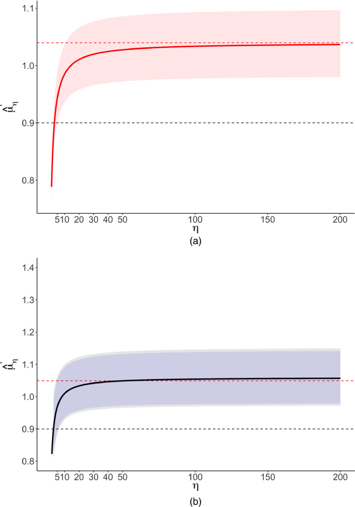
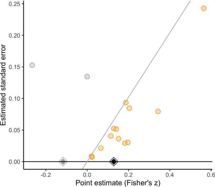
Fig. 2 shows a significance funnel plot, which suggests a positive correlation between the point estimates and their standard errors. Our methods apply under the assumption that such correlation arises from selection due to publication bias rather than to correlation between the point estimates and standard errors in the underlying population. To estimate the severity of publication bias that is required to attenuate or to the null and to a non‐null correlation of 0.10, we used the analytic results in Section 3.1 for the common effect specification. For the two random‐effects specifications, we conducted a grid search across values of η between 1 and 200 (Fig. 3). The second and third columns of Table 2 indicate that, for all three model specifications, no amount of publication bias under the assumed model could attenuate the observed point estimate or even its lower CI limit to the null. The last two columns indicate that, when considering the non‐null value q ′=0.10, extreme publication bias (η=11 or η=28 depending on whether common effect or robust meta‐analysis is used) or substantial publication bias (from η=3 to η=5) would be capable of attenuating the estimate or the lower bound of its CI, , to a correlation of 0.10. Thus, overall, we might conclude that, regardless of the severity of publication bias, this meta‐analysis provides strong evidence for an average effect in the observed direction, albeit possibly of small size.
Figure 2.
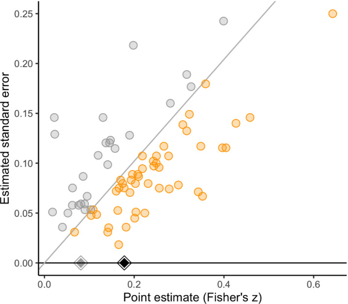
Significance funnel plot for the video games meta‐analysis of Anderson et al. (2010) (point estimates are on Fisher's z‐scale, the scale on which p‐values were computed; studies lying on the diagonal line have p=0.05): , non‐affirmative; , affirmative; , robust clustered estimate in non‐affirmative studies only; , robust clustered estimate in all studies
Figure 3.
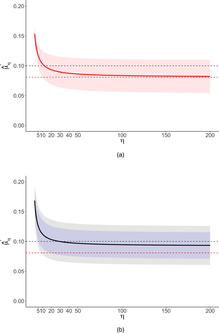
Corrected point estimates and CIs for the video games meta‐analysis of Anderson et al. (2010) as a function of η ( , non‐null value q
′;
, non‐null value q
′;  , worst‐case estimates): (a) common effect specification; (b) robust specifications (
 , CI assuming independence;
  , CI allowing for clustering)
Table 2.
Severity of publication bias, S, in Anderson et al. (2010) required to attenuate or to the null or to q ′=0.10 on Pearson's r‐scale†
| Model |
|
|
|
|
||||
|---|---|---|---|---|---|---|---|---|
| Common effect | Not possible | Not possible | 11 | 4 | ||||
| Robust (independent) | Not possible | Not possible | 28 | 5 | ||||
| Robust (clustered) | Not possible | Not possible | 28 | 3 |
†‘Not possible’ indicates that no value of η could sufficiently attenuate the statistic. Values are conservatively rounded down to the nearest integer.
7.2. PI3K/AKT/mTOR inhibitors and progression‐free cancer survival
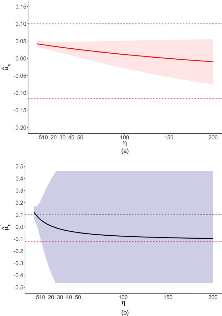
A second meta‐analysis assessed the effect of PI3K/AKT/mTOR inhibitors on progression‐free survival from advanced solid cancers (Li et al., 2018). The meta‐analysis comprised 50 randomized controlled studies contributed by 39 papers and found that PI3K/AKT/mTOR inhibitors improved progression‐free survival compared with various control therapies (hazard ratio HR = 0.79; 95% CI [0.71, 0.88]). To conduct our sensitivity analyses, we assumed that publication bias would favour studies showing a protective effect of PI3K/AKT/mTOR inhibitors, so, as described in Section 4, we first reversed the signs of all point estimates on the log‐hazard scale. We transformed the results back to the hazard ratio scale and took inverses so that, in all results that we report, HR<1 indicates a protective effect of PI3K/AKT/mTOR inhibitors as in the original meta‐analysis. When conducting sensitivity analyses with a non‐null effect size threshold, we set q=− log (0.90)≈ log (1.1) in analysis to consider attenuating the point estimate on the original scale ( ) to a hazard ratio of q ′=0.90.
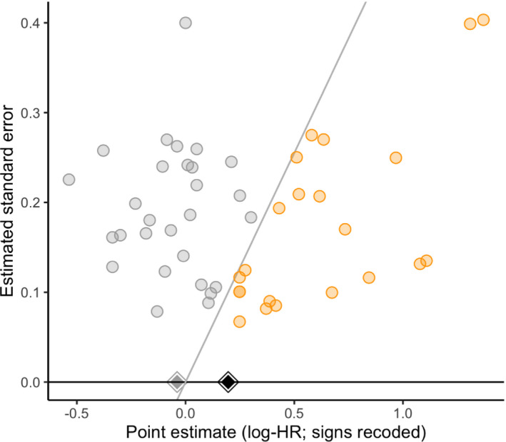
Fig. 4 shows a significance funnel plot, Table 3 shows uncorrected and worst‐case point estimates, Table 4 shows and for two choices of q, and Fig. 5 shows as a function of η. The worst‐case point estimates were close to the null and in the opposite direction from the original estimate for all three model specifications (e.g. 1.03 with 95% CI [0.94, 1.12] for the robust clustered specification). Considerable publication bias would be required to shift the point estimate of 0.79 to the null ( for the robust clustered specification). However, only moderate publication bias would be required to shift the upper CI limit to the null ( ) or to shift the point estimate to a non‐null value of 0.90 ( ).
Figure 4.
Significance funnel plot for the cancer meta‐analysis of Li et al. (2018) (studies lying on the diagonal line have p=0.05): , non‐affirmative; , affirmative; , robust clustered estimate in non‐affirmative studies only; , robust clustered estimate in all studies
Table 3.
Uncorrected and worst‐case point estimates (HR) for the cancer meta‐analysis of Li et al. (2018)
| Model |
|
CI for
|
|
CI for
|
||||
|---|---|---|---|---|---|---|---|---|
| Uncorrected | ||||||||
| Common effect | 0.79 | [0.76, 0.82] | — | — | ||||
| Standard† | 0.79 | [0.71, 0.89] | 0.36 | [0.26, 0.44] | ||||
| Robust (independent) | 0.80 | [0.71, 0.89] | — | — | ||||
| Robust (clustered) | 0.82 | [0.74, 0.91] | — | — | ||||
| Worst case | ||||||||
| Common effect | 1.04 | [0.98, 1.10] | ||||||
| Robust (independent) | 1.05 | [0.97, 1.14] | ||||||
| Robust (clustered) | 1.03 | [0.94, 1.12] | ||||||
†Standard: parametric random‐effects meta‐analysis assuming independence, included for comparison. and its CI are presented on the log(HR)‐scale, the scale on which the data were analysed.
Table 4.
Severity of publication bias, S, in Li et al. (2018) required to attenuate or (the upper limit of the CI for ) to the null or to q ′=0.90†
| Model |
|
|
|
|
||||
|---|---|---|---|---|---|---|---|---|
| Common effect | 14 | 5 | 3 | 2 | ||||
| Robust (independent) | 8 | 2 | 2 | 1 | ||||
| Robust (clustered) | 8 | 2 | 2 | 1 |
†‘1’ indicates that the statistic is already greater than or equal to q ′. Values are conservatively rounded down to the nearest integer.
Figure 5.
Corrected point estimates (HR) and CIs for the cancer meta‐analysis of Li et al. (2018) as a function of η (, non‐null value q
′; , worst‐case estimates): (a) common effect specification; (b) robust specifications (, CI assuming independence; , CI allowing for clustering)
Li et al. (2018) had concluded that there was ‘no significant publication bias’ (p=0.23) on the basis of Egger's test, which assumes that publication bias operates on point estimate size rather than statistical significance and does not affect the largest studies, and that effects are not heterogeneous. However, our sensitivity analyses suggest that the conclusions may be sensitive to plausible degrees of publication bias, such as publication bias in which affirmative studies are twice as likely to be published as non‐affirmative studies. The significance funnel plot in Fig. 4 helps to clarify the discrepancy: although the point estimates do not appear to be correlated with their standard errors (as Egger's test assesses), the estimates in the non‐affirmative studies are typically close to the null or even in the unexpected direction, so publication bias that favours affirmative results could potentially attenuate the meta‐analytic estimate considerably.
7.3. Optimism and dietary quality
A third meta‐analysis assessed the association between optimism and several health behaviours (Boehm et al., 2018). We focus here on the meta‐analysis for dietary quality, which included 15 studies (eight cross‐sectional and seven longitudinal) contributed by 13 papers and found that optimism was associated with a small improvement in dietary quality (r=0.12; 95% CI [0.08, 0.16]). Boehm et al. (2018) reported that a standard trim‐and‐fill sensitivity analysis left the estimate and its CI unchanged, yet applying a selection model (Andrews and Kasy, 2019) reversed its direction (Pearson's r,−0.11; 95% CI [−0.30, 0.09]). This meta‐analysis also serves as an interesting test case because its small size (and, in particular, its inclusion of only two non‐affirmative studies) warrants considerable circumspection about the results of both trim‐and‐fill and standard selection models.
We conducted our sensitivity analyses as for the meta‐analysis on video games of Anderson et al. (2010). Fig. 6 shows a significance funnel plot. Like the results of Boehm et al. (2018) by using a standard selection model, our worst‐case estimates (−0.12 for all specifications; Table 5) are in the opposite direction from the observed point estimate. However, because these worst‐case estimates are based on meta‐analysing only two non‐affirmative studies, the robust CIs are, quite reasonably, almost completely uninformative (e.g. [−0.95, 0.92] for both random‐effect specifications); this suggests that the narrower asymptotic CI from the selection model (i.e. 95% CI [−0.30, 0.09]) may be anticonservative for this small meta‐analysis. Sensitivity analyses across multiple values of η (Table 6 and Fig. 7) suggested that, under the two random‐effects specifications, fairly considerable publication bias (η=3 or η=4) could attenuate and its lower CI limit to the null or to a correlation of 0.10.
Figure 6.
Significance funnel plot for the optimism meta‐analysis (studies lying on the diagonal line have p=0.05): , non‐affirmative; , affirmative; , robust clustered estimate in non‐affirmative studies only; , robust clustered estimate in all studies
Table 5.
Uncorrected and worst‐case point estimates (Pearson's r) for the optimism meta‐analysis of Boehm et al. (2018)
| Model |
|
CI for
|
|
CI for
|
||||
|---|---|---|---|---|---|---|---|---|
| Uncorrected | ||||||||
| Common effect | 0.04 | [0.03, 0.05] | — | — | ||||
| Standard† | 0.12 | [0.06, 0.18] | 0.08 | [0.00, 0.11] | ||||
| Robust (independent) | 0.12 | [0.06, 0.17] | — | — | ||||
| Robust (clustered) | 0.13 | [0.07, 0.19] | — | — | ||||
| Worst case | ||||||||
| Common effect | −0.12 | [−0.30, 0.08] | ||||||
| Robust (independent) | −0.12 | [−0.95, 0.92] | ||||||
| Robust (clustered) | −0.12 | [−0.95, 0.92] | ||||||
†Standard: parametric random‐effects meta‐analysis assuming independence, included for comparison. and its CI are presented on Fisher's z‐scale, the scale on which the data were analysed.
Table 6.
Severity of publication bias, S, in Boehm et al. (2018) required to attenuate or to the null or to q ′=0.10 on Pearson's r‐scale†
| Model |
|
|
|
|
||||
|---|---|---|---|---|---|---|---|---|
| Common effect | 148 | 49 | 1 | 1 | ||||
| Robust (independent) | 22 | 4 | 3 | 1 | ||||
| Robust (clustered) | 22 | 4 | 3 | 1 |
†‘1’ indicates that the statistic is already less than or equal to q ′. Values are conservatively rounded down to the nearest integer.
Figure 7.
Corrected point estimates (Pearson's r) and CIs for the optimism meta‐analysis as a function of η (, non‐null value q
′; , worst‐case estimates): (a) common effect specification; (b) robust specifications ( CI assuming independence; , CI allowing for clustering)
These analyses therefore indicate that, although we can draw some conclusions regarding the sensitivity of these results to mild publication bias, considerable uncertainty remains regarding the effect of severe publication bias. However, unlike inference for standard selection models, our proposed methods of inference perform nominally even for small meta‐analyses with few non‐affirmative studies (see Section 8 for simulation results). Thus, the wide CIs for large values η may nevertheless be informative; they indicate that there simply is not enough information in this meta‐analysis to provide any reasonable assurance that the results are robust to moderate or severe publication bias.
8. Simulation study
We assessed the performance of our proposed sensitivity analyses under the three model specifications and in a variety of realistic and extreme scenarios, including those with quite small sample sizes. We considered three categories of scenarios:
-
a
those with homogeneous population effects, for which we applied the common effect specification,
-
b
those with heterogeneous independent population effects, for which we used the robust independent specification and
-
c
those with heterogeneous clustered population effects, for which we used the robust clustered specification.
For each of 1000–1500 simulation iterates per scenario, we first generated an underlying population of studies before introducing publication bias. The underlying population comprised M * clusters (potentially with no intercluster heterogeneity, depending on the scenario) of five studies each; note that 5M * represents the number of studies in the underlying population, but the number of published studies that were actually meta‐analysed was often much smaller after the introduction of publication bias, as described below. We generated studies’ point estimates according to either a normal or an exponential random‐intercepts specification such that the total heterogeneity across studies was τ 2, comprising an intercluster heterogeneity of var(ζ) and an intracluster heterogeneity of τ 2−var(ζ). Continuing our convention of using asterisks to denote study‐specific variables and parameters in the underlying population,
In a full factorial design, we varied the parameters M *, μ, τ 2 and var(ζ), as well as the distribution of the study level random effects ( ), across the values in Table 7. We simulated a scenario for each combination of values in Table 7 except those with both τ 2=0 and var(ζ)=0.5, which would have had τ 2−var(ζ)<0. Thus, scenarios with τ 2=0 and var(ζ)=0 were common effect specifications, those with τ 2=1 and var(ζ)=0 were independent random‐effects specifications and those with τ 2=1 and var(ζ)=0.5 were clustered random‐effects specifications.
Table 7.
Possible values of simulation parameters
| η | M * | μ | τ 2 | var(ζ) | γ‐distribution | Additional | |
|---|---|---|---|---|---|---|---|
| selection | |||||||
|
on
|
|||||||
| 1 | 20 | 0.20 | 0 | 0 | Normal | No | |
| 10 | 40 | 0.80 | 1 | 0.50 | Exponential | Yes | |
| 20 | 80 | ||||||
| 50 | 200 | ||||||
| 100 |
We then introduced publication bias as in Section 2.2, varying η from 1 (no publication bias) to 100 (extreme publication bias). The effective sample size on which the precision of our methods depends most strongly is the number of published non‐affirmative studies, so we ensured that our choices of M * and η resulted in numerous scenarios in which the median number of published non‐affirmative studies was less than 10 and sometimes as small as 1. On the basis of τ 2 and var(ζ), we fit the correctly specified fixed or random‐effects model, using the true η to estimate and its 95% CI. Additionally, as described in Section 2.2, our proposed sensitivity analyses can be applied without modification in certain situations in which the publication process not only favours affirmative studies but also favours both affirmative and non‐affirmative studies with small standard errors. To confirm this result, we also ran all the above simulation scenarios with this more complicated publication process.
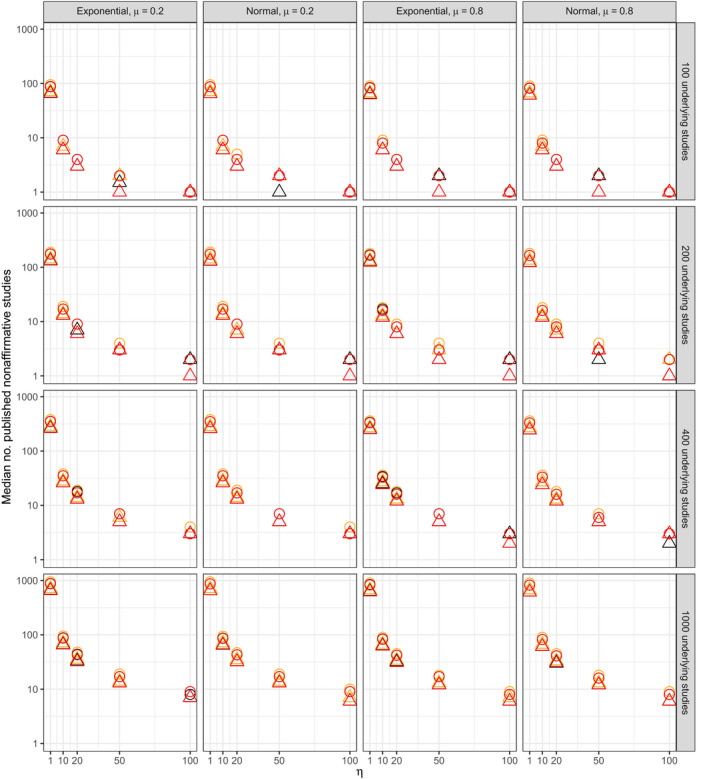
Figs 8 and 9 respectively show the median numbers of published studies and of published non‐affirmative studies for all 480 simulation scenarios. Fig. 10 shows that was approximately unbiased for scenarios with η⩽20. The bias increased somewhat under extreme publication bias (e.g. η=100), though the coverage remained nominal for all scenarios (mean 96% and minimum 93% across all scenarios). Table 8 shows the median width of 95% CIs for , showing the expected patterns of dependence on the number of published non‐affirmative studies and on the severity of publication bias. Also as expected theoretically, results from scenarios in which the publication process also favoured small standard errors yielded results comparable with those of scenarios in which the publication process favoured only affirmative studies, except in so far as the former publication process resulted in smaller numbers of published studies.
Figure 8.
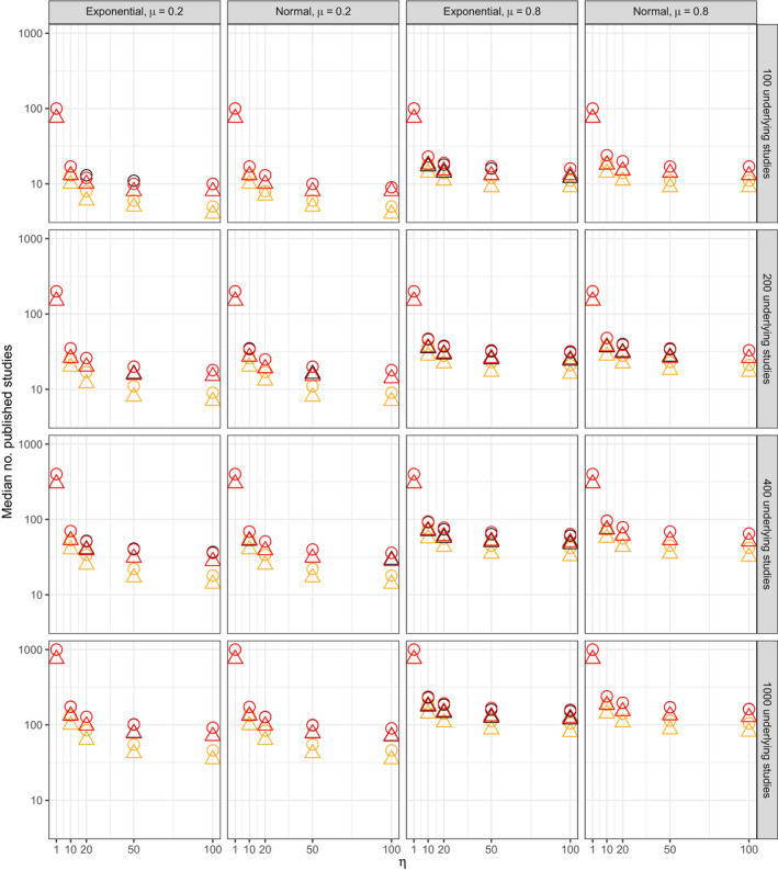
Median number of published studies across all simulation iterates (rows, numbers of studies in the underlying population before publication bias (5M
*); columns, distributions of study level random effects and true mean μ):  , not selected on standard error;
  , selected for small standard error;
  , common effect;
  , robust clustered;
  , robust independent
Figure 9.
Median number of published non‐affirmative studies across all simulation iterates (rows, numbers of studies in the underlying population before publication bias (5M
*); columns, distribution of study level random effects and true mean μ): , not selected on standard error; , selected for small standard error; , common effect; , robust clustered; , robust independent
Figure 10.
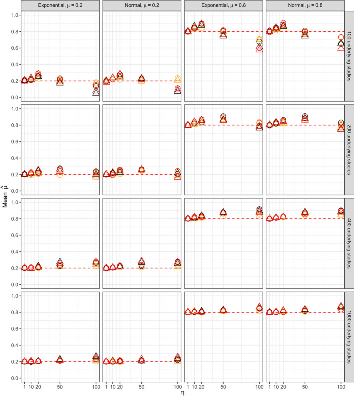
Mean point estimate across simulation iterates (rows, number of studies in the underlying population before publication bias (5M
*); columns, distribution of study level random effects and true mean μ): , μ; , not selected on standard error; , selected for small standard error; , common effect; , robust clustered; , robust independent
Table 8.
Median width of CI for by the median number of published non‐affirmative studies in the simulation scenario ( ) and η
|
Median
|
η | Median CI width | |
|---|---|---|---|
| ⩾10 | 1† | 0.40 | |
| 10 | 0.86 | ||
| 20 | 0.96 | ||
| 50 | 1.19 | ||
| 100 | 1.49 | ||
| <10 | 10 | 1.97 | |
| 20 | 2.30 | ||
| 50 | 3.33 | ||
| 100 | 4.23 |
†Among scenarios with η=1, all had a median of 10 or more published non‐affirmative studies.
9. Alternative models of publication bias
Throughout, we have considered a one‐tailed model of publication bias in which ‘significant’ results with positive point estimates are favoured, whereas significant results with negative point estimates and ‘non‐significant’ results are equally disfavoured. We have also assumed that results are selected for publication based on a single p‐value cut‐off at p=0.05. This section discusses our rationale for these modelling choices and describes how our results could be easily extended to accommodate other models of publication bias.
Whereas we assumed one‐tailed selection, it is possible instead that significant results are favoured regardless of direction, whereas only non‐significant results are disfavoured (called ‘two‐tailed’ selection). Although our methods can be trivially modified for two‐tailed selection, as described below, we speculate that one‐tailed selection is more realistic in many scientific contexts. For many research questions, only effects in the positive direction are scientifically marketable, whereas both negative and null results are interpreted as a failure to support the marketable hypothesis (e.g. Vevea et al. (1993)). Even in controversial realms, in which some investigators try to prove a given hypothesis while others try to disprove it, non‐significant and negative results may be comparably interpreted as failing to support the hypothesis at stake. For example, we suspect that this may be so for the literature on violent video games, which has tended to interpret results suggesting beneficial effects of violent video games primarily as failures to support hypothesized detrimental effects, rather than as support for a priori less plausible benefits. Indeed, the distributions of p‐values in the meta‐analyses that were included in the empirical study of Section 6 usually appeared to conform well to one‐tailed selection (Mathur and VanderWeele, 2020a).
Some areas of research may, however, exhibit two‐tailed selection. For example, if there are two scientifically marketable hypotheses at stake, each predicting results in a different direction, then perhaps publication bias would equally favour significant positive results and significant negative results. In such cases, one could conduct our proposed sensitivity analyses under two‐tailed selection simply by redefining , such that all significant studies, regardless of direction, receive weights of 1, whereas only non‐significant studies receive weights of η. However, we nevertheless recommend by default conducting sensitivity analyses under a one‐tailed selection model, even when there is reason to suspect some degree of two‐tailed selection, because assuming one‐tailed selection is often (though not always) conservative in the sense that it leads to smaller than assuming two‐tailed selection. Specifically, conservatism holds when the inverse‐probability‐weighted, meta‐analytic estimate among only the non‐significant studies and affirmative studies combined is at least as large as the meta‐analytic estimate among only the significant negative studies, for which a sufficient condition is that the common effect mean in the non‐significant studies is positive (on‐line supplement, section 1.2). (However, this conservatism does not necessarily hold for the analogous metric pertaining to the lower bound of the CI for the pooled estimate, .)
Note also that we modelled selection by using a single cut‐off at p=0.05 both for ease of interpretation and because it conforms well to empirical findings on how applied researchers and statisticians interpret and report p‐values (Head et al., 2015; Masicampo and Lalande, 2012; McShane and Gal, 2017). In principle, other cut‐offs might also be relevant; for example, ‘marginally significant’ findings with 0.05<p<0.10 might have an intermediate publication probability. However, in practice, experimental evidence suggests that researchers do not distinguish much between two different p‐values both falling above or below the major 0.05 cut‐off (McShane et al., 2016). Our proposed sensitivity analyses could be modified for multiple cut‐offs simply by defining more than two groups of studies, each with a distinct publication probability, and again weighting each study by its inverse publication probability (as in, for example, Hedges (1992)). However, by introducing multiple free sensitivity parameters, this approach would less readily yield straightforward single‐number summaries of the severity of publication bias that are required to explain away the results.
10. Discussion
This paper has proposed sensitivity analyses for bias due to selective publication and reporting in meta‐analyses. These sensitivity analyses shift the focus from estimating the severity of publication bias to quantifying the amount of publication bias that would be required to attenuate the observed point estimate, or its lower CI limit, to the null or to a chosen non‐null value. This shift in focus enables particularly simple statements regarding sensitivity to publication bias that would be easy to report in meta‐analyses. Our metric S(t,q) describes the amount of publication bias that is required to attenuate the meta‐analytic statistic t (i.e. either the pooled point estimate or its lower CI limit) to a smaller value q. If this sensitivity parameter is sufficiently small that it represents a plausible amount of publication bias (perhaps informed by the empirical benchmarks that we have provided), then the meta‐analysis may be considered relatively sensitive to publication bias. In contrast, if S(t,q) represents an implausibly large amount of publication bias, then one might consider the meta‐analysis to be relatively robust. The methods proposed can sometimes indicate that no amount of publication bias under the model assumed could explain away the results of a meta‐analysis, providing a compelling argument for robustness. In contrast with existing methods for sensitivity analysis, the present methods can accommodate non‐normal population effects, small meta‐analyses and non‐independent point estimates. All methods are implemented in the R package PublicationBias (described in the on‐line supplement, section 2).
These methods have limitations. Although they relax distributional assumptions on the population effects, they do assume a particular model of publication bias that is chosen to align with empirical evidence on how researchers interpret p‐values. We have suggested some simple diagnostics to assess the plausibility of some of these assumptions (Section 4). If publication bias departs considerably from this model, e.g. because studies with large effects rather than merely p<0.05 are favoured, the analyses proposed may be compromised. However, for perhaps the most plausible violation of our modelling assumptions (namely, two‐tailed instead of one‐tailed selection), we have shown that our assumptions are often, though not always, conservative at least when considering the point estimate. Additionally, some meta‐analyses may not contain any non‐affirmative studies because, for example, the population effects are very large or publication bias is extremely severe; in these cases, our methods cannot be applied because there would be no non‐affirmative studies to upweight. Also, it is important to note that sensitivity to publication bias does not imply that publication bias is actually severe in practice; nor the converse. Last, our sensitivity analyses characterize evidence strength by using the standard meta‐analytic point estimate and its CI, but these metrics alone do not fully characterize evidence strength in a potentially heterogeneous distribution of effects (Mathur and VanderWeele, 2018). Other metrics may be useful additional targets of sensitivity analysis (Mathur and VanderWeele, 2018, 2020b) but would require bias correction for as well as, which proved challenging under publication bias in meta‐analyses of realistic sizes (on‐line supplement, section 3).
In summary, we have proposed sensitivity analyses for publication bias in meta‐analyses that are straightforward to conduct and intuitive to interpret. These methods can be easily implemented by using the R package PublicationBias, and we believe that their widespread reporting would help to calibrate confidence in meta‐analysis results.
11. Reproducibility
All code required to reproduce the applied examples and simulation study is publicly available and documented (https://osf.io/7wc2t/). Data from the Boehm et al. (2018) and Li et al. (2018) meta‐analyses are publicly available (linked at https://osf.io/7wc2t/). Data from the meta‐analysis of Anderson et al. (2010) cannot be made public at the author's request, but they will be made available on request to individuals who have secured permission from Craig Anderson.
Supporting information
‘Supplement: Sensitivity analysis for publication bias in meta‐analyses’.
Acknowledgements
Craig Anderson provided raw data for reanalysis and answered analytic questions. Zachary McCaw contributed to the proof of theorem 1.1 (supplement, section 1.1). Zachary Fisher provided helpful discussion regarding his R package robumeta. The participants of the Harvard University Applied Statistics Workshop provided many insightful comments and suggestions. This research was supported by National Institutes of Health grant R01 CA222147 and John E. Fetzer Memorial Trust grant R2020‐16; the funders had no role in the conduct or reporting of this research.
References
- Anderson, C. A. , Shibuya, A. , Ihori, N. , Swing, E. L. , Bushman, B. J. , Sakamoto, A. , Rothstein, H. R. and Saleem, M. (2010) Violent video game effects on aggression, empathy, and prosocial behavior in Eastern and Western countries: a meta‐analytic review. Psychol. Bull., 136, 151–173. [DOI] [PubMed] [Google Scholar]
- Andrews, I. and Kasy, M. (2019) Identification of and correction for publication bias. Am. Econ. Rev., 109, 2766–2794. [Google Scholar]
- Bergmann, C. , Tsuji, S. , Piccinini, P. E. , Lewis, M. L. , Braginsky, M. , Frank, M. C. and Cristia, A. (2018) Promoting replicability in developmental research through meta‐analyses: insights from language acquisition research. Chld Devlpmnt, 89, 1996–2009. [DOI] [PMC free article] [PubMed] [Google Scholar]
- Boehm, J. K. , Chen, Y. , Koga, H. , Mathur, M. B. , Vie, L. L. and Kubzansky, L. D. (2018) Is optimism associated with healthier cardiovascular‐related behavior?: Meta‐analyses of 3 health behaviors. Circuln Res., 122, 1119–1134. [DOI] [PubMed] [Google Scholar]
- Bom, P. R. and Rachinger, H. (2019) A kinked meta‐regression model for publication bias correction. Res. Synth. Meth., 10, 497–514. [DOI] [PubMed] [Google Scholar]
- Brockwell, S. E. and Gordon, I. R. (2001) A comparison of statistical methods for meta‐analysis. Statist. Med., 20, 825–840. [DOI] [PubMed] [Google Scholar]
- Chan, A.‐W. , Hróbjartsson, A. , Haahr, M. T. , G⊘tzsche, P. C. and Altman, D. G. (2004) Empirical evidence for selective reporting of outcomes in randomized trials: comparison of protocols to published articles. J. Am. Med. Ass., 291, 2457–2465. [DOI] [PubMed] [Google Scholar]
- Coursol, A. and Wagner, E. E. (1986) Effect of positive findings on submission and acceptance rates: a note on meta‐analysis bias. Professnl Psychol. Res. Pract., 17, no. 2, 136–137. [Google Scholar]
- Dear, K. B. and Begg, C. B. (1992) An approach for assessing publication bias prior to performing a meta‐analysis. Statist. Sci., 7, 237–245. [Google Scholar]
- Ding, P. and VanderWeele, T. J. (2016) Sensitivity analysis without assumptions. Epidemiology, 27, no. 3, 368–377. [DOI] [PMC free article] [PubMed] [Google Scholar]
- Duval, S. and Tweedie, R. (2000) Trim and fill: a simple funnel‐plot-based method of testing and adjusting for publication bias in meta‐analysis. Biometrics, 56, 455–463. [DOI] [PubMed] [Google Scholar]
- Egger, M. , Smith, G. D. , Schneider, M. and Minder, C. (1997) Bias in meta‐analysis detected by a simple, graphical test. Br. Med. J., 315, 629–634. [DOI] [PMC free article] [PubMed] [Google Scholar]
- Ferguson, C. J. and Kilburn, J. (2010) Much ado about nothing: the misestimation and overinterpretation of violent video game effects in eastern and western nations; Comment on Anderson et al. (2010). Psychol. Bull., 136, 174–178. [DOI] [PubMed] [Google Scholar]
- Field, A. P. and Gillett, R. (2010) How to do a meta‐analysis. Br. J. Math. Statist. Psychol., 63, 665–694. [DOI] [PubMed] [Google Scholar]
- Fisher, Z. and Tipton, E. (2015) Robumeta: an R‐package for robust variance estimation in meta‐analysis. Preprint arXiv:1503.02220. University of North Carolina at Chapel Hill, Chapel Hill.
- Franco, A. , Malhotra, N. and Simonovits, G. (2014) Publication bias in the social sciences: unlocking the file drawer. Science, 345, 1502–1505. [DOI] [PubMed] [Google Scholar]
- Greenwald, A. G. (1975) Consequences of prejudice against the null hypothesis. Psychol. Bull., 82, 1–20. [Google Scholar]
- Head, M. L. , Holman, L. , Lanfear, R. , Kahn, A. T. and Jennions, M. D. (2015) The extent and consequences of p‐hacking in science. PLOS Biol., 13, no. 3, article e1002106. [DOI] [PMC free article] [PubMed] [Google Scholar]
- Hedges, L. V. (1992) Modeling publication selection effects in meta‐analysis. Statist. Sci., 7, 246–255. [Google Scholar]
- Hedges, L. V. , Tipton, E. and Johnson, M. C. (2010) Robust variance estimation in metaregression with dependent effect size estimates. Res. Synth. Meth., 1, 39–65. [DOI] [PubMed] [Google Scholar]
- Hilgard, J. , Engelhardt, C. R. and Rouder, J. N. (2017) Overstated evidence for short‐term effects of violent games on affect and behavior: a reanalysis of Anderson et al. (2010). Psychol. Bull., 143, no. 7. [DOI] [PubMed] [Google Scholar]
- Ioannidis, J. P. and Trikalinos, T. A. (2007) The appropriateness of asymmetry tests for publication bias in meta‐analyses: a large survey. Can. Med. Ass. J., 176, 1091–1096. [DOI] [PMC free article] [PubMed] [Google Scholar]
- Jin, Z.‐C. , Zhou, X.‐H. and He, J. (2015) Statistical methods for dealing with publication bias in meta‐analysis. Statist. Med., 34, 343–360. [DOI] [PubMed] [Google Scholar]
- Johnson, V. E. , Payne, R. D. , Wang, T. , Asher, A. and Mandal, S. (2017) On the reproducibility of psychological science. J. Am. Statist. Ass., 112, 1–10. [DOI] [PMC free article] [PubMed] [Google Scholar]
- Kepes, S. , Bushman, B. J. and Anderson, C. A. (2017) Violent video game effects remain a societal concern: Reply to Hilgard, Engelhardt, and Rouder (2017). Perspect. Psychol. Sci., 143, no. 7, 775–782. [DOI] [PubMed] [Google Scholar]
- Lee, K. P. , Boyd, E. A. , Holroyd‐Leduc, J. M. , Bacchetti, P. and Bero, L. A. (2006) Predictors of publication: characteristics of submitted manuscripts associated with acceptance at major biomedical journals. Med. J. Aust., 184, 621–626. [DOI] [PubMed] [Google Scholar]
- Lewis, M. , Braginsky, M. , Tsuji, S. , Bergmann, C. , Piccinini, P. E. , Cristia, A. and Frank, M. C. (2017) Quantitative synthesis of early language acquisition using meta‐analysis. Preprint (Available from https://psyarxiv.com/htsjm.)
- Li, X. , Dai, D. , Chen, B. , Tang, H. , Xie, X. and Wei, W. (2018) Efficacy of PI3K/AKT/mTOR pathway inhibitors for the treatment of advanced solid cancers: a literature‐based meta‐analysis of 46 randomised control trials. PLOS One, 13, no. 2, article e0192464. [DOI] [PMC free article] [PubMed] [Google Scholar]
- Masicampo, E. and Lalande, D. R. (2012) A peculiar prevalence of p values just below .05. Q. J. Exptl Psychol., 65, 2271–2279. [DOI] [PubMed] [Google Scholar]
- Mathur, M. B. and VanderWeele, T. J. (2018) New metrics for meta‐analyses of heterogeneous effects. Statist. Med., 38, 1336–1342. [DOI] [PMC free article] [PubMed] [Google Scholar]
- Mathur, M. B. and VanderWeele, T. J. (2020a) Estimating publication bias in meta‐analyses: a meta‐meta‐analysis across disciplines and journal tiers. Preprint Quantitative Sciences Unit, Stanford University, Stanford. (Available from https://osf.io/p3xyd/.)
- Mathur, M. B. and VanderWeele, T. J. (2020b) Robust metrics and sensitivity analyses for meta‐analyses of heterogeneous effects. Epidemiology, 31, 356–358. [DOI] [PMC free article] [PubMed] [Google Scholar]
- McShane, B. B. , Böckenholt, U. and Hansen, K. T. (2016) Adjusting for publication bias in meta‐analysis: an evaluation of selection methods and some cautionary notes. Perspect. Psychol. Sci., 11, 730–749. [DOI] [PubMed] [Google Scholar]
- McShane, B. B. and Gal, D. (2017) Statistical significance and the dichotomization of evidence. J. Am. Statist. Ass., 112, 885–895. [DOI] [PMC free article] [PubMed] [Google Scholar]
- Olson, C. M. , Rennie, D. , Cook, D. , Dickersin, K. , Flanagin, A. , Hogan, J. W. , Zhu, Q. , Reiling, J. and Pace, B. (2002) Publication bias in editorial decision making. J. Am. Med. Ass., 287, 2825–2828. [DOI] [PubMed] [Google Scholar]
- Orwin, R. G. (1983) A fail‐safe n for effect size in meta‐analysis. J. Educ. Statist., 8, no. 2, 157–159. [Google Scholar]
- Peters, J. L. , Sutton, A. J. , Jones, D. R. , Abrams, K. R. and Rushton, L. (2008) Contour‐enhanced meta‐analysis funnel plots help distinguish publication bias from other causes of asymmetry. J. Clin. Epidem., 61, 991–996. [DOI] [PubMed] [Google Scholar]
- Rice, K. , Higgins, J. P. T. and Lumley, T. (2018) A re‐evaluation of fixed effect(s) meta‐analysis. J. R. Statist. Soc. A, 181, 205–227. [Google Scholar]
- Rosenthal, R. (1979) The file drawer problem and tolerance for null results. Psychol. Bull., 86, 638–641. [Google Scholar]
- Schmidt, F. L. and Hunter, J. E. (2014) Methods of Meta‐analysis: Correcting Error and Bias in Research Findings. New York: Sage. [Google Scholar]
- Stanley, T. D. and Doucouliagos, H. (2014) Meta‐regression approximations to reduce publication selection bias. Res. Synth. Meth., 5, 60–78. [DOI] [PubMed] [Google Scholar]
- Sterne, J. A. , Gavaghan, D. and Egger, M. (2000) Publication and related bias in meta‐analysis: power of statistical tests and prevalence in the literature. J. Clin. Epidem., 53, 1119–1129. [DOI] [PubMed] [Google Scholar]
- Tipton, E. (2015) Small‐sample adjustments for robust variance estimation with meta‐regression. Psychol. Meth., 20, no. 3, 375–393. [DOI] [PubMed] [Google Scholar]
- VanderWeele, T. J. and Ding, P. (2017) Sensitivity analysis in observational research: introducing the E‐value. Ann. Intern. Med., 167, 268–274. [DOI] [PubMed] [Google Scholar]
- VanderWeele, T. J. , Mathur, M. B. and Ding, P. (2019) Correcting misinterpretations of the e‐value. Ann. Intern. Med., 170, 131–132. [DOI] [PubMed] [Google Scholar]
- Vevea, J. L. , Clements, N. C. and Hedges, L. V. (1993) Assessing the effects of selection bias on validity data for the general aptitude test battery. J. Appl. Psychol., 78, 981–987. [Google Scholar]
- Vevea, J. L. and Hedges, L. V. (1995) A general linear model for estimating effect size in the presence of publication bias. Psychometrika, 60, 419–435. [Google Scholar]
- Vevea, J. L. and Woods, C. M. (2005) Publication bias in research synthesis: sensitivity analysis using a priori weight functions. Psychol. Meth., 10, 428–443. [DOI] [PubMed] [Google Scholar]
- Viechtbauer, W. (2005) Bias and efficiency of meta‐analytic variance estimators in the random‐effects model. J. Educ. Behav. Statist., 30, 261–293. [Google Scholar]
- Viechtbauer, W. (2010) Conducting meta‐analyses in R with the metafor package. J. Statist. Softwr., 36, no. 3, 1–48. [Google Scholar]
- Wang, C.‐C. and Lee, W.‐C. (2019) A simple method to estimate prediction intervals and predictive distributions: summarizing meta‐analyses beyond means and confidence intervals. Res. Synth. Meth, 10, 255–266. [DOI] [PubMed] [Google Scholar]
- Wooldridge, J. M. (2007) Inverse probability weighted estimation for general missing data problems. J. Econmetr., 141, 1281–1301. [Google Scholar]
Associated Data
This section collects any data citations, data availability statements, or supplementary materials included in this article.
Supplementary Materials
‘Supplement: Sensitivity analysis for publication bias in meta‐analyses’.