Abstract
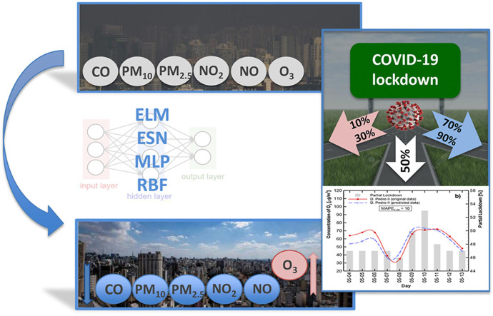
Studies have reported significant reductions in air pollutant levels due to the COVID-19 outbreak worldwide global lockdowns. Nevertheless, all of the reports are limited compared to data from the same period over the past few years, providing mainly an overview of past events, with no future predictions. Lockdown level can be directly related to the number of new COVID-19 cases, air pollution, and economic restriction. As lockdown status varies considerably across the globe, there is a window for mega-cities to determine the optimum lockdown flexibility. To that end, firstly, we employed four different Artificial Neural Networks (ANN) to examine the compatibility to the original levels of CO, O3, NO2, NO, PM2.5, and PM10, for São Paulo City, the current Pandemic epicenter in South America. After checking compatibility, we simulated four hypothetical scenarios: 10%, 30%, 70%, and 90% lockdown to predict air pollution levels. To our knowledge, ANN have not been applied to air pollution prediction by lockdown level. Using a limited database, the Multilayer Perceptron neural network has proven to be robust (with Mean Absolute Percentage Error ∼ 30%), with acceptable predictive power to estimate air pollution changes. We illustrate that air pollutant levels can effectively be controlled and predicted when flexible lockdown measures are implemented. The models will be a useful tool for governments to manage the delicate balance among lockdown, number of COVID-19 cases, and air pollution.
Keywords: Artificial neural networks, SARS-CoV-2, Air pollution, Lockdown flexibility
Graphical abstract
Highlights
-
•
COVID-19 cases, air pollution and lockdown level inter-dependency can be predicted.
-
•
First time ANN application to predict air quality change as a function of lockdown.
-
•
MLP has proven to be robust, with mean absolute percentage error around 30%.
-
•
Hypothetical lockdown (10–90%) predicted CO, O3, NO2, NO, PM2.5 and PM10 levels.
Artificial Neural Networks showed to be robust predictive tools to estimate the best equilibrium among COVID-19 cases, lockdown percentage, and air pollutants level.
1. Introduction
The World Health Organization (WHO) stated that South America is the new epicenter of the coronavirus pandemic (CNBC, 2020), and Brazil, one of the countries with the highest incidence of new cases and the second highest total number of cases in the world. A study done by scientists from Imperial College, London, showed that Brazil had the highest rate of transmission (R0 of 2.81) among the 48 countries they investigated (The Lancet, 2020). To date (September 3, 2020), 6.6% of Brazil’s total cases (3,997,865) were recorded in São Paulo city (262,570). This number constitutes more than 30% of the cases reported in São Paulo state (826,331). On September the 3rd the number of deaths in São Paulo city was 11,554 (4.4% of confirmed cases of COVID-19 led to death), higher than the global (3.3%) (SEADE, 2020).
Due to the rapid person-to-person transmission of COVID-19, São Paulo state government ordered lockdown on March 24, 2020, closing all (Secondary schools, Universities, Shopping Malls and, other commercial entities) but essential services (Nakada and Urban, 2020). As expected, beyond the efficiency to suppress the R0 (Wilder-Smith and Freedman, 2020), these actions led to the scaling down in traffic, industrial and trade activities, and consequent reduction in air pollution levels, therefore improving air quality as a whole (Dutheil et al., 2020).
In response to the exponential increase in infection rates of the virus worldwide, local and national governments relaxed environmental legislation. For instance, the US EPA allowed industries and other facilities autonomy to decide and report if they meet the legislated requirements (Wu et al., 2020). Similarly, the Brazilian government has largely negated enforcement of environmental legislation during the coronavirus outbreak (The Guardian, 2020), which resulted in additional industrial air pollution emission, as well as, an increase in deforestation in the Amazon (de Oliveira et al., 2020). The danger is that reduced enforcement will continue past virus’s peak to stimulate the economy and therefore put the population at risk.
Various scientists reported decreased air pollutant levels, comparing pre- and post COVID-19 air pollution levels using different methods and scales (Chauhan and Singh 2020; Dantas et al., 2020; Le et al., 2020; Li et al., 2020; Muhammad et al., 2020; Nakada and Urban, 2020; Sharma et al., 2020; Shehzad et al., 2020; Tobías et al., 2020). However, the available air pollution studies related to the COVID-19 situation are based on satellite images, air quality modeling and generally comparing lockdown period data with monthly means over the past few years. Worldwide, most studies reported in the literature indicated reductions in NOx and PM2.5 levels and an increase in O3 concentration during lockdown (Nakada and Urban, 2020; Sharma et al., 2020; Sicard et al., 2020; Siciliano et al., 2020; Tobías et al., 2020). The following are a few examples of studies using these approaches.
Many researchers worldwide reported a reduction in NO2 concentration levels (Chauhan and Singh, 2020; Muhammad et al., 2020; Zambrano-Monserrate et al., 2020). Zambrano-Monserrate et al. (2020) reported reductions in China, USA, Italy, and Spain, when Copernicus Atmosphere Monitoring Service data for PM2.5 and NO2 were compared to the previous three years. Rodríguez-Urrego and Rodríguez-Urrego (2020) studied PM2.5 profiles of the 50 most polluted countries and reported an average reduction of 12% worldwide. They used the World Air Quality Index platform to obtain data and compared it to the previous 2 years.
Closer to home, Dantas et al. (2020) and Nakada and Urban (2020) compared various air pollutants (including CO, O3, NO2, NO, PM2.5, PM10, and SO2) over different time scales (one year to five-year trend) in Rio de Janeiro and São Paulo, respectively. In both cases, local data were used. Both studies indicated a reduction of all pollutants investigated, except for ozone, which increased.
These approaches (using satellite images, air quality modeling and generally comparing lockdown period data with monthly means over the past few years) are limited as it provides mainly an overview of past events, with no future predictions.
Artificial Neural Networks (ANN), on the other hand, is a nonlinear methodology capable of mapping a set of inputs into an output, which is important to support decisions regarding preventive measures. This approach has been used in air pollution epidemiological studies (Araujo et al., 2020; Kachba et al., 2020; Kassomenos et al., 2011; Tadano et al., 2016; Polezer et al., 2018). In Araujo et al. (2020) and Kassomenos et al. (2011), the ANN showed a better performance than linear approaches as Generalized Linear Models. Kassomenos et al. (2011) also concluded that ANN is a more flexible and adaptive mathematical approach.
In this context, as lockdown status varies considerably across the globe, there is a window of opportunity for mega-cities to determine the optimum level of lockdown to ensure effective management of transmission rates, air quality, and a healthy economy. To our knowledge, ANN have not been applied to air pollution prediction by lockdown level.
To that end, we used four Artificial Neural Networks (ANN) (Extreme Learning Machine – ELM; Echo State Network – ESN; Multilayer perceptron – MLP and Radial Basis Function Networks – RBF) to estimate the influence that newly reported COVID-19 cases and lockdown level may have on the local air pollution (CO, O3, NO2, NO, PM2.5, and PM10 levels) in São Paulo city. After checking compatibility, we simulated four hypothetical partial lockdown scenarios (10, 30, 70, and 90%) to investigate the relationship between reduced activities and air quality.
In the light of evidence that poor air quality may exacerbate COVID-19 symptoms (Wu et al., 2020), and potentially lead to higher mortality rates, the ANN showed to be a useful predictive tool for governments. Using this approach, resumption of industrial and other activities can be managed to ensure a sustainable balance among economic health, air quality, and transmission rate.
2. Materials and methods
The data of São Paulo city was selected to examine the robustness of our approach. São Paulo is the most populous city of Latin America, with around 12.25 million inhabitants (IBGE, 2020), the main hotspot of COVID-19 in Brazil, and one of the most polluted cities in Latin America. The inputs were: daily number of COVID-19 cases, partial lockdown level, and meteorological variables; the outputs were the daily concentration of each air pollutant (CO [ppm], O3 [μg/m3], NO2 [μg/m3], NO [μg/m3], PM2.5 [μg/m3], and PM10 [μg/m3]).
Data on the daily number of newly reported COVID-19 cases and lockdown percentages was collected from March 17, 2020 to May 13, 2020 from the Statistical Portal of São Paulo State (SEADE, 2020). The Intelligence Monitoring System of São Paulo has an agreement with mobile phone companies to track people’s movement. This georeferenced anonymised information is available on the SEADE website and has been used in this study.
Meteorological variables were extracted from the Environmental Company of São Paulo State database (CETESB). These included: relative humidity – RH [%]; maximum temperature – MT [oC]; atmospheric pressure – AP [hPA]; wind speed – WS [m/s] and global solar radiation–GSR [W/m2]) (CETESB, 2020).
The data on target pollutant levels of CO [ppm], O3 [μg/m3], NO2 [μg/m3], NO [μg/m3], PM2.5 [μg/m3], and PM10 [μg/m3] concentrations were selected from January 01, 2020 to May 13, 2020 (134 samples). As a matter of comparison and to improve the ANN performance, we included the data for a period with zero COVID-19 cases and no lockdown (data from January 01, 2020 to March 16, 2020).
Daily concentrations were extracted from the CETESB. More than sixty-six percent of the hourly averages were similar to the daily average. The data were ratified by the CETESB, who follows the quality assurance/quality control (QA/QC) procedure approved by the State Council of Environment (CONSEMA) of the State of São Paulo. Beta radiation is used for PM10 and PM2.5 measurements, chemiluminescence for NO2 and NO, non-dispersive infrared for CO, and ultraviolet analysis for O3 (CETESB, 2020).
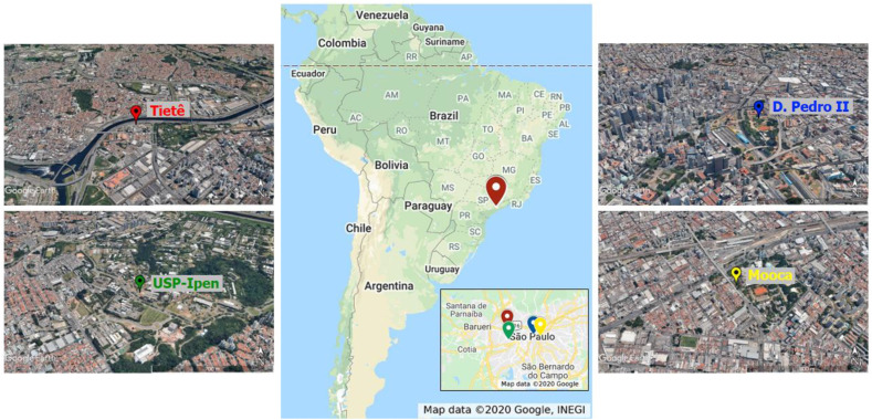
Data from four CETESB air quality monitoring stations (AQMS) were used due to their locations (Fig. 1 ). The largest data sets could be obtained from D. Pedro II station (blue spot - located in a high demographic density area) and Tietê station (red spot located near a busy ring road). D. Pedro II station is located downtown – high demographic density area; influenced mainly by a light-duty fleet, and Tietê station is near a ring road, characterized mainly by heavy-duty emissions.
Fig. 1.
Locations of the air quality monitoring stations in São Paulo. The satellite map is from Google Maps (Map data©2020 Google; https://www.google.com/maps/place/Brazil/); the satellite is from Google Earth Pro (Map data©2020 Google; www.google.com/maps/@-23.6815315,-46.8754814,10z). The maps were edited with Microsoft Power Point (version 16.28–19081202). Note: AQMS: Air Quality Monitoring Station; Tietê: ring road; D. Pedro II: downtown; ∗Tietê station has no O3 data and was replaced by data from USP-Ipen station.
Table 1 shows that even at these two stations, some data is lacking. PM2.5 data from D. Pedro II station had several gaps in the data set for consecutive days, and these were replaced by data from Mooca station (yellow spot) (CETESB, 2020), as the linear correlation of the data with those from D. Pedro II station is 0.95. For missing data from non-consecutive days, the previous day’s values were used. Tietê station had no ozone data, and it was supplemented by data from a nearby location USP-Ipen station (green spot).
Table 1.
Number of days with no data for each studied AQMS.
| AQMS | CO | O3 | NO2 | NO | PM10 | PM2.5 |
|---|---|---|---|---|---|---|
| Tietê∗ | 2 | 0∗ | 0 | 0 | 1 | 2 |
| D. Pedro II | 4 | 1 | 0 | 0 | 0 | 10 |
Note: AQMS: Air Quality Monitoring Station; Tietê: ring road; D. Pedro II: downtown; ∗ Tietê station has no O3 data and was replaced by data from USP-Ipen station.
2.1. Artificial Neural Networks
The four ANN used in this study are described below (further details in Araujo et al. (2020)).
2.1.1. Multilayer Perceptron overview
The Multilayer Perceptron (MLP) is a neural model able to map any nonlinear, continuous, limited, and differentiable function with arbitrary precision, which confers a characteristic of a universal approximator (Haykin, 2008). The basic structure of an ANN is the artificial neurons, functional units responsible for processing the information, and providing the output response (de Castro, 2007).
In an MLP, the neurons are distributed in three kinds of layers. The input layer transmits the data to the intermediate (hidden) layers, where the neurons perform a nonlinear transformation, mapping the input signal to another space. Then, the signal is sent to the output layer, in which the output signal is generated based on a linear combination, in most cases. Neurons from the same layer are disconnected, while those from disjoint layers fully exchange information since this is a feed forward model (Siqueira and Luna, 2019).
Training a neural model means using an algorithm to determine its free parameters or adjust the neurons’ weights. The most known way to solve this task in an MLP is to use the backpropagation algorithm, a general iterative tool based on the steepest descent, a first order unrestricted linear optimization method. In this case, the method reduces the mean square error between the desired response and the output of the network (Haykin, 2008). However, in this work, we address a second-order method that presents computational cost similar to the first: The Modified Scaled Conjugate Gradient (MSCG) (dos Santos and Von Zuben, 1999).
We highlight the maximum number of iterations as the stop criterion in training. We also use the hold-out cross-validation method to determine the topology (number of neurons in the hidden layer) and avoid overfitting (Haykin, 2008).
2.1.2. Radial basis function
The Radial Basis Function networks (RBF) are a well-known ANN model. Like the MLP, they are feed forward architectures, and universal approximators, but present only two layers of neurons (Siqueira and Luna, 2019). The first, intermediate, perform a nonlinear input-output mapping using radial basis functions, like the Gaussian function. The second – output layer –performs the model’s response, similarly to the MLP (Haykin, 2008).
The hidden neurons present two parameters: a centre c i (with the same dimension of the number of inputs), and a dispersion σ i Therefore, the output of each neuron is higher to inputs that are spatially closer to the current centre. The dispersion is responsible for modulating the decay of the response concerning the distance between the inputs and the centers. Usually, the Gaussian function is addressed as RBF. A linear combinator is used to perform the output response (Siqueira and Luna, 2019).
The training process of an RBF is performed in two steps. The first is the adjustment of the hidden neurons (centers and dispersions), a task performed by the unsupervised clustering method. In this work, we addressed the K-Medoids algorithm. Also, we assumed that all dispersions are the same (Haykin, 2008). The second step is the adjustment of the output neurons. A simple and efficient tool found in the literature is the use of the Moore–Penrose inverse operator (Haykin, 2008).
2.1.3. Extreme Learning Machines
Extreme Learning Machines (ELM) are feed forward neural models, with a single hidden layer (Huang et al., 2006, 2015). This structure is quite similar to the classic MLP, the training process being the main difference (Siqueira et al., 2018).
In an ELM, the intermediate neurons have weights randomly generated, and they are not adjusted during the running time. The insertion of new neurons in the hidden layer leads to a decrease in the output error (Siqueira et al., 2012a).
Then, an ELM training is summarized in finding the best set of weights of the output layer. The main manner to overcome this task is to use a minimum square solution, especially the Moore–Penrose generalized inverse operation (Siqueira et al., 2018).
2.1.4. Echo State Networks
The Echo State Networks (ESN) are architectures of ANN, which present high similarity with the ELM, regarding the structure and training process. However, unlike the previously mentioned networks, this is a recurrent model since it presents feedback loops of information. In this case, the hidden layer, named dynamic reservoir, has such recurrence (Jaeger, 2001, 2002).
Jaeger (2001, 2002) demonstrated that the reservoir is a nonlinear transformation, which is influenced by the recent samples of the input signal, so that we can choose the weights in advance if specific conditions are respected. In this work, we used the reservoir design by (Jaeger, 2001).
As in the ELM, the training is responsible for determining the weights of the output layer, which may be done using the Moore–Penrose generalized inverse operation, as in the ELM case (Siqueira et al., 2018).
2.2. Computational details
The computational step involved the seven input variables mentioned above: number of COVID-19 new cases, partial lockdown level, maximum temperature, relative humidity, atmospheric pressure, wind speed, and global solar radiation. The desired signals (target) were each air pollutant’s (CO, O3, NO2, NO, PM2.5, and PM10) concentration.
We evaluated the performance considering all the inputs at the same time; without the number of new COVID-19 cases; and without the number of new COVID-19 cases and partial lockdown, to analyze the robustness of the neural networks on predicting air quality according to COVID-19 variables and using a small database. All cases included the meteorological variables.
To perform the computational analysis, we separated the dataset in three subsets:
-
•
Training: from January 01 to April 23, 2020 (114 samples);
-
•
Validation: April 24 to May 03, 2020 (10 samples);
-
•
Test: May 04 to May 13, 2020 (10 samples).
The training subset is used to adjust the models, and the validation is applied to verify the overtraining and define the number of neurons in the intermediate layer. Finally, the test subset is used to evaluate the performance of the models. We also verified if the use of the Z-score may bring some performance gain. It is a mathematical treatment that transforms the series of data into approximately stationary. Some studies have presented the importance of using such an approach (Kachba et al., 2020; Siqueira et al., 2018).
To apply the Z-score, the value of each sample is subtracted from the mean and divided by the standard deviation. At the end of the ANN execution, the process is reversed to analyze the performances in the original domain.
The number of neurons in the hidden layer was defined by empirical tests, varying from 3 to 100 neurons. The best number for each case was chosen based on the lower Mean Square Error (MSE) in the test set. The number of neurons in the hidden layer of each neural model is in Table A1, Table A2 in Appendix A.
We followed the premises from the literature of adopting the MSE as the most important error metric because this is reduced during the training (adjustment) of the neural models (Araujo et al., 2020; Kachba et al., 2020; Siqueira et al., 2014, 2018, 2020).
The artificial neurons in the intermediate layer of the MLP, ELM, and ESN, use the hyperbolic tangent as an activation function. In the RBF, the Gaussian function is used. The MLP training addressing the Modified Scaled Conjugate Gradient (MSCG) and uses as stop criterion the maximum number of 500 iterations. Also, the K-Medoids in RBF achieved the stop criterion after 10 iterations without modification in the position of the centroids (Figueiredo et al., 2019).
3. Results and discussion
For simplicity, we divided this section into three parts. Firstly, the descriptive analysis of the databases, followed by the ANN prediction results, and lastly, the results for the hypothetical scenarios of 10%, 30%, 70%, and 90% of lockdown.
3.1. Descriptive analysis
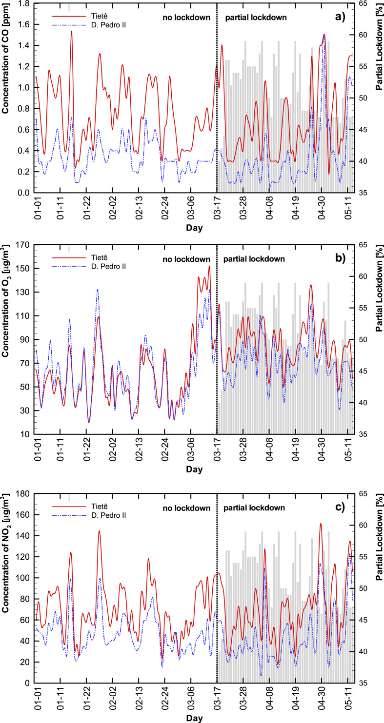
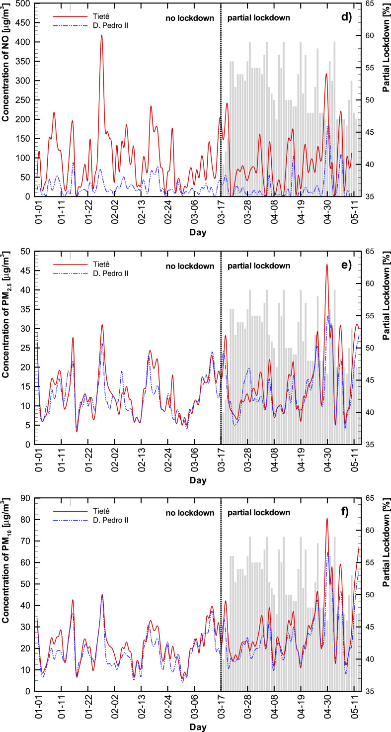
The daily concentrations during the studied period, together with the partial lockdown level, are shown in Appendix A - Figure A1. The São Paulo state government officially ordered lockdown on March 24, 2020, however, the population started to self-isolate voluntarily the week before (first available social isolation data – March 17, 2020). From March 17, 2020 to May 13, 2020, the lockdown varied between 38 and 59%, with an average of 51%.
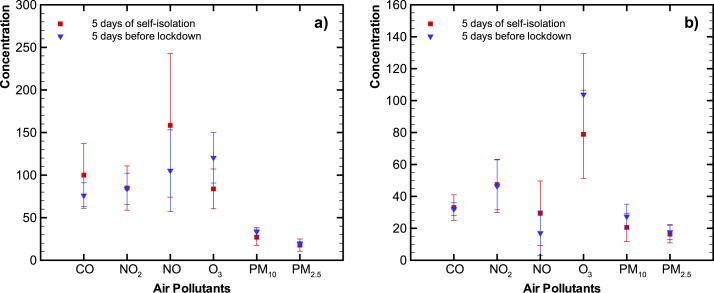
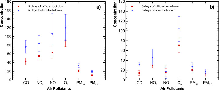
To visualize changes in air pollution levels due to voluntary self-isolation and/or lockdown, we compared the five-day average before (12–16 March 2020) voluntary self-isolation with a five-day average during self-isolation (17–21 March 2020) (Fig. 2 ). There is no distinctive change in pollutant levels within experimental error, as may be expected due to a lag in response and a low level of reduced activities. However, comparing a five-day average during the first lockdown period (54–56% lockdown from 24 to 28 of March 2020) with the period before lockdown or self-isolation, we do observe a general decrease in pollutant levels for all pollutants at Tietê and for most at D. Pedro II as is shown in Fig. 3 . As this period would reflect the changes in the self-isolation period’s activities with additional reduction of activities, this finding is not surprising.
Fig. 2.
Five-day average pollutant levels before and during the voluntary self-isolation period at Tietê station (a) and D. Pedro II station (b) (CO concentration were multiplied by 100).
Fig. 3.
Averages comparison between five days of official lockdown with five days before lockdown for Tietê station (a) and D. Pedro II station (b) (CO concentration were multiplied by 100).
From Figure A1 we observe that this trend continues until around the 24th of April, after which relaxation in lockdown rules corresponds to a steady increase in most of the pollutant levels. It does seem as though not all the pollutants are similarly influenced by the lockdown. The particulate matter concentration appears to be influenced by other factors as well, and reaches much higher values towards the end of the lockdown period discussed here than what it was before. The ozone levels generally increased with a lockdown percentage increase.
Using a neural network to study atmospheric ozone formation in the Metropolitan Area of São Paulo (MASP), Guardani et al. (1999) found that temperature was the main factor affecting ozone formation and observed higher ozone levels in regions characterized by lower emission levels of ozone precursors. Martins and Andrade (2008) evaluated VOC s’ potential for ozone formation using a three-dimensional air quality model and found that ozone in the MASP is VOC-limited, as commonly observed in urban areas (Li et al., 2019; Siciliano et al., 2020; Tobías et al., 2020). Under these conditions, a decrease of NOx can reduce the removal of O3 through NOx titration and/or the effect of radical terminating reactions, and thereby increasing O3 formation (Seinfeld and Pandis, 2016; Sillman, 1999, 2003). Furthermore, Andrade et al. (2017), studying the MASP, explain that decreasing NOx and CO emissions simultaneously contribute to higher ozone levels. This behavior is also affirmed in (Gentner et al., 2009; Harley et al., 2005; Marr and Harley, 2002; Stedman, 2004).
Table 2 presents the linear correlations between the lockdown level (varying from 38 to 59%) and air pollutant concentrations at Tietê and D. Pedro II stations for March 17, 2020 (first day of available data of social isolation) to May 13, 2020. Bar ozone, all the pollutants correlated negatively (ranging from −0.14 for CO at D. Pedro II to −0.60 for NO at Tietê) with the lockdown.
Table 2.
Linear correlations between lockdown and studied air pollutant concentrations for March 17, 2020 to May 13, 2020.
| CO | O3∗ | NO2 | NO | PM10 | PM2.5 | |
|---|---|---|---|---|---|---|
| Tietê | −0.45 | 0.15 | −0.57 | −0.60 | −0.34 | −0.38 |
| D. Pedro II | −0.14 | 0.11 | −0.42 | −0.33 | −0.23 | −0.26 |
Note: ∗Data from USP-Ipen station.
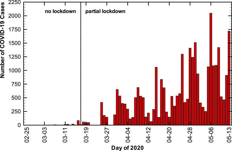
Finally, Appendix A - Figure A2 shows the number of daily COVID-19 newly reported cases. The first day of registered COVID-19 cases was February 25, 2020 and an exponential increase is observed from the beginning of April onwards.
3.2. ANN estimation analysis
Table 3, Table 4 contain the average and standard deviation for each pollutant level obtained from the 3 subsets (training, validation, and test) at the two sites. Although the two monitoring sites are in the same city, the descriptive statistics show significant differences. Tietê station (near highways) has higher average concentrations for all pollutants in comparison to D. Pedro II station (populated city area). The different statistical profiles of the two sites are indicative of robust evaluation of the data, as the model could provide a MAPE of ∼30%, despite two dissimilar data sets.
Table 3.
Average and standard deviation for each studied pollutant for the 3 subsets (Tietê Station).
| Training |
Validation |
Test |
||||
|---|---|---|---|---|---|---|
| Pollutant | Average | Standard Deviation | Average | Standard Deviation | Average | Standard Deviation |
| CO [ppm] | 0.69 | 0.29 | 0.93 | 0.46 | 0.85 | 0.34 |
| O3[μg/m3] | 70 | 28 | 98 | 21 | 74 | 14 |
| NO2[μg/m3] | 68 | 24 | 86 | 31 | 88 | 31 |
| NO [μg/m3] | 91 | 69 | 124 | 89 | 151 | 84 |
| PM2.5[μg/m3] | 13 | 5.5 | 24 | 12 | 20 | 9.7 |
| PM10[μg/m3] | 22 | 8.2 | 43 | 19 | 38 | 19 |
Table 4.
Average and standard deviation for each studied pollutant for the 3 subsets (D. Pedro II Station).
| Training |
Validation |
Test |
||||
|---|---|---|---|---|---|---|
| Pollutant | Average | Standard Deviation | Average | Standard Deviation | Average | Standard Deviation |
| CO [ppm] | 0.30 | 0.15 | 0.62 | 0.40 | 0.50 | 0.36 |
| O3[μg/m3] | 65 | 24 | 81 | 19 | 59 | 14 |
| NO2[μg/m3] | 43 | 17 | 60 | 33 | 64 | 31 |
| NO [μg/m3] | 21 | 19 | 51 | 63 | 75 | 76 |
| PM2.5[μg/m3] | 12 | 4.7 | 20 | 8.8 | 16 | 7.8 |
| PM10[μg/m3] | 19 | 7.3 | 37 | 14 | 31 | 16 |
Table A1, Table A2 (Appendix A) display the ANN computational results for AQMS Tietê (ring road station) and AQMS D. Pedro II (densely populated city area station), respectively. For this purpose, the best (lower Mean Square Error - MSE) of 30 independent executions were considered (de Castro, 2007; Haykin, 2008; Siqueira et al., 2018). The shaded values indicate results with the best performance (lower MSE). The MLP neural model achieved the best results (i.e., lowest MSE) in almost all cases, except for O3 at D. Pedro II station. The latter was best estimated using the ELM neural model. It is an important observation, as there is no consensus about which ANN is the best. It corroborates with the results achieved by Polezer et al. (2018) and Araujo et al. (2020), both applied to air pollution epidemiological studies.
It is important to highlight that the best overall ANN results were achieved when the variables “number of new COVID-19 cases” and “partial lockdown” were included (8 out of 12 cases). The remaining 4 cases (NO2 and PM2.5 at Tietê, and NO2 and O3 at D. Pedro II) showed the best result considering only “partial lockdown”. In both scenarios the meteorological variables were included.
To establish if the Z-Score application could result in performance gain, the ANN was also performed with the Z-score (Results shown in Table A1, Table A2). The Z-score’s use proved to be beneficial in 2 cases at the Marginal Tietê station, and four cases at the D. Pedro II site. Therefore, it can be considered in addition to increasing the quality of the results of the ANN.
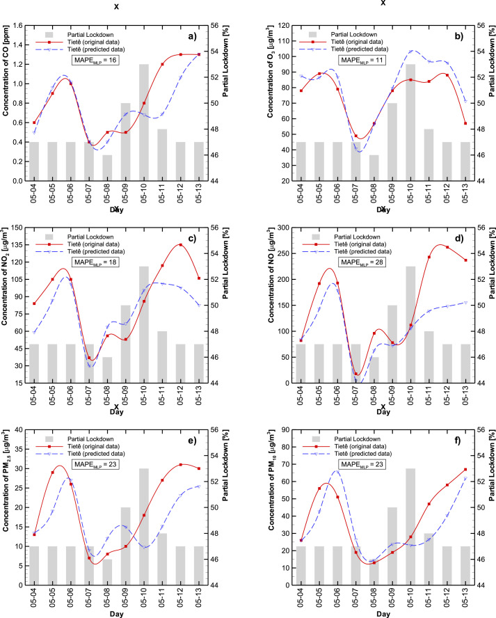
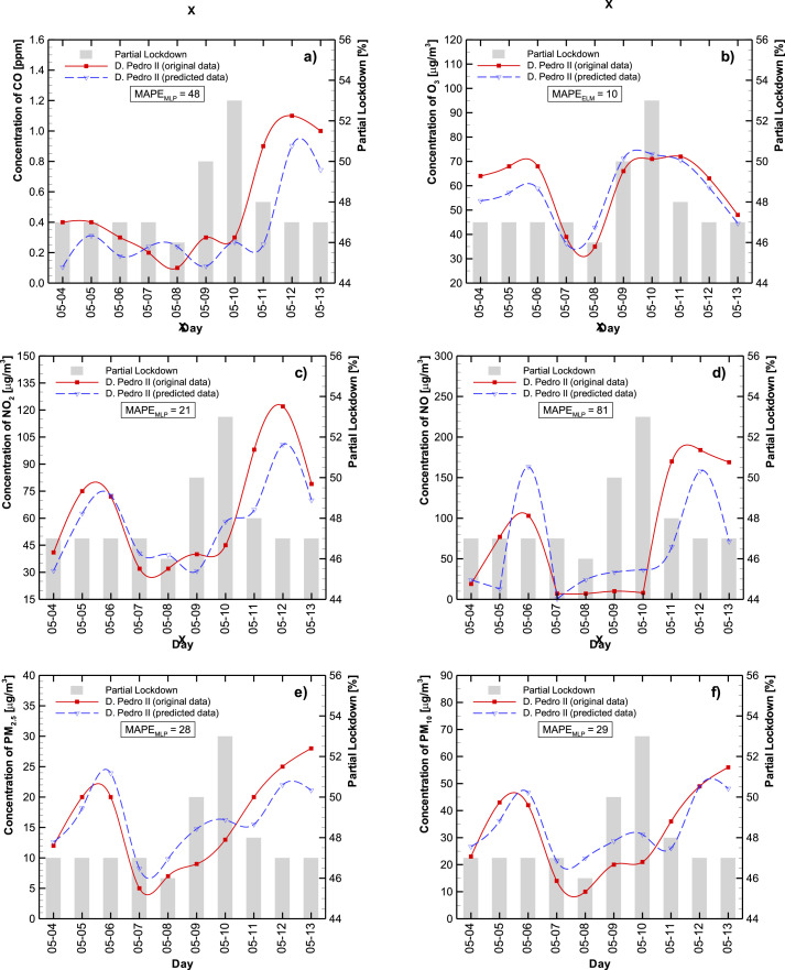
Fig. 4, Fig. 5 represent the observed (continuous red line) and best estimation (dashed blue line) concentration levels for CO (a), O3 (b), NO2 (c), NO (d), PM2.5 (e), and PM10 (f) at Tietê and D. Pedro II stations, respectively during the period 4–13 May 2020. The lockdown level is indicated as shaded bars.
Fig. 4.
Best estimation to predict CO (a), O3 (b), NO2 (c), NO (d), PM2.5 (e), and PM10 (f) levels for Tietê station. Predictions are in dashed lines and observed levels in solid lines. The bars are the partial lockdown.
Fig. 5.
Best estimation to predict CO (a), O3 (b), NO2 (c), NO (d), PM2.5 (e), and PM10 (f) levels for D. Pedro II station. Predictions are in dashed lines and observed levels in solid lines. The bars are the partial lockdown.
In general, the predicted results, using this approach, captured the original data tendencies reasonably well, with a mean absolute percentage error (MAPE) of 30% for almost all cases. The exceptions were at D. Pedro II station (CO – 48% and NO - 81%) (see Table A1, Table A2 – Appendix A).
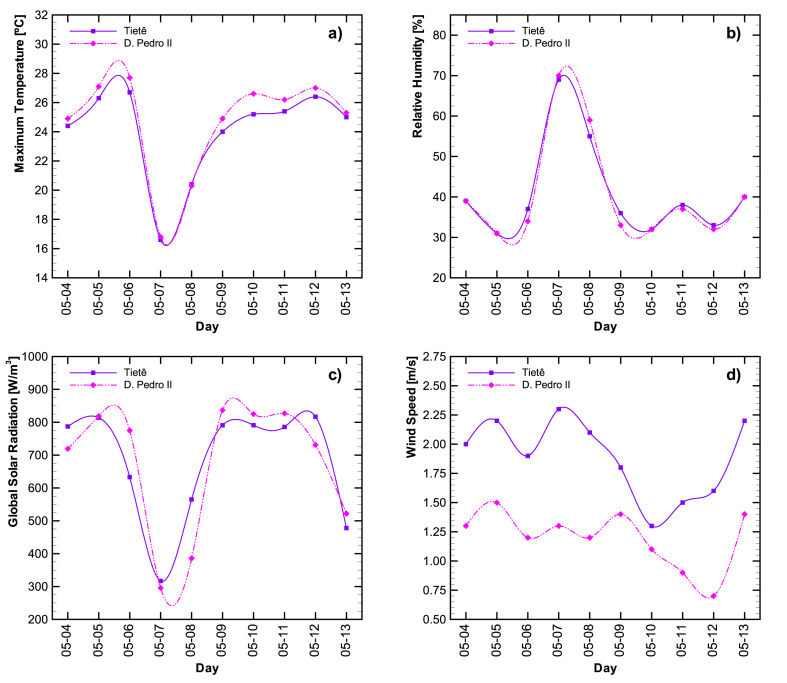
It is important to notice two distinct behaviors during the lockdown to the test set period (see Fig. 4, Fig. 5). When the lockdown level remains unchanged (first 5 days), the main influence can be ascribed to the meteorological variables (Figure A3 – shows the meteorological raw data for the test period). But after five days in the test set, the percentage lockdown jumps from 46% to 53% in two days. As the temperature and relative humidity were relatively stable in the last five days, one can say that the lockdown is the main contributor to the change in air pollutant level. Observe that ozone concentration has a consistent relation with solar irradiation, with similar profiles. This behavior is in accordance with those observed at the beginning of lockdown (March 17, 2020), as mentioned in section 3.1. The importance of maintaining continuous and consistent interventions to curb air pollution is evident from the data displayed here. It is particularly important during extreme air pollution events, and there is enough evidence that lockdown measures will nearly instantly reduce air pollution levels.
Each ANN architecture has positive and negative points. As discussed in Section 2.1, the ESN is a recurrent model, presenting feedback loops of information in its hidden layer. This characteristic may be relevant when dealing with data processing since more information is available to form the output response. Additionally, together with the ELM, their training processes require less computational effort than the RBF and MLP, since there are no iterative processes to adjust their weights because the hidden layer is not modified. In addition, other works have presented the capability of such models to overcome traditional, fully trained architectures (Araujo et al., 2020; Siqueira et al., 2012a, 2014, 2018).
Despite the advantage and good results found in the literature for ESN, ELM, and RBF (Siqueira et al., 2012b, 2018), the MLP errors were smaller than the others. It seems clear that adjusting the hidden weights is an important step in nonlinear mapping applications, as is presented in this investigation. In this case, there are a set of inputs of variable nature (for example, temperature, humidity, and partial lockdown), and mapping these values to another variable is not a trivial task (Kachba et al., 2020; Polezer et al., 2018).
3.3. Hypothetical scenarios
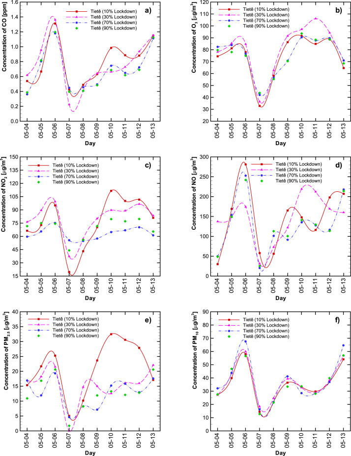
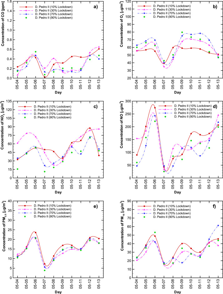
To predict the impact that the partial lockdown has on air quality, four hypothetical scenarios were modeled: a minimum lockdown level (10%); possible vertical isolation (only for COVID-19 high-risk groups – over-60s and people with chronic disease, diabetics, among others) (30%); the considered ideal lockdown percentage (70%); and an extreme isolation action (90%). The results are compared in Fig. 6, Fig. 7 , with results for AQMS Tietê D. Pedro II, respectively. The red lines correspond to 10% lockdown, the pink lines to 30% lockdown, the blue lines to 70% lockdown, and the green lines to 90% lockdown. The pollutant designation (a -f) is the same as for Fig. 4, Fig. 5.
Fig. 6.
Hypothetical scenarios considering the impact that 10% (red line), 30% (pink like), 70% (blue line), and 90% (green line) lockdown would have on CO (a), O3 (b), NO2 (c), NO (d), PM2.5 (e), and PM10 (f) levels for AQMS Tietê. (For interpretation of the references to colour in this figure legend, the reader is referred to the Web version of this article.)
Fig. 7.
Hypothetical scenarios considering the impact that 10% (red line), 30% (pink like), 70% (blue line), and 90% (green line) lockdown would have on CO (a), O3 (b), NO2 (c), NO (d), PM2.5 (e), and PM10 (f) levels for AQMS D. Pedro II. (For interpretation of the references to colour in this figure legend, the reader is referred to the Web version of this article.)
The data in Fig. 6 (Tietê station) indicates that in general higher concentrations are predicted for all pollutants at 10 (red line) and 30 (pink line) % lockdown. A different pattern is observed for May 07 and May 08, whereby the lower lockdown also predicted low pollutant concentrations. During these two days, the meteorological conditions changed abruptly (low temperature and solar irradiation, and high relative humidity - see Figure A3). This scenario exemplifies the complex interdependency of air pollutant levels on several variables. These findings suggest that when abrupt weather conditions are forecasted, lockdown interventions should happen a few days earlier. Our data corroborate with the recent publication of Hong et al. (2019) who reported that extreme weather events might be a crucial mechanism by which air quality is influenced.
The predicted ozone concentration at Tietê station (Fig. 6b) for the 30% lockdown showed an unexpected behavior, presenting higher concentrations than 70% and 90% lockdown. It may have been a consequence of the complexity of the variables that influence air quality. Although this may be seen as a poor fit for the model, we need to emphasize that this is one case out of twelve.
Although the same abrupt change in meteorological conditions was observed for 7 and 8 May at the D. Pedro II station (Fig. 7), the ANN could estimate the response more coherently than for the Tietê station. This may be due to other factors at play, influencing the air pollutant level at this station. Observe that the ozone profiles are as expected, especially for a 10% lockdown. It is important to highlight that the ANN prediction was good as only one of the seven inputs were changed.
We also observe that the particulate matter levels are not greatly influenced by lockdown (as reported by Nakada and Urban, 2020), especially the PM10 concentration. At the D. Pedro II station, the PM2.5 levels also stay very similar regardless of the lockdown level.
We acknowledge that air pollutant levels have a complex set of variables that determine it, and that even a powerful tool such as ANN cannot always accurately predict the level. However, the data presented here provides adequate evidence that ANN can be used successfully to estimate the impact of different levels of lockdown will have on the air quality.
4. Conclusion
Artificial Neural Networks were able to predict how changes in the level of lockdown affected air quality in São Paulo City. We have shown that even when using a restricted data set of pollutant levels together with meteorological information, the ANN results showed Mean Absolute Percentage Error (MAPE) around 30%.
The result of the ANN approach to four hypothetical scenarios of lockdown (i.e., 10%, 30%, 70%, and 90%) showed evidence of the complexity of the calculation problem as a consequence of the abrupt meteorological changes.
For the first time, ANN were used as a tool to describe the equilibrium between air pollution, COVID-19 cases, and the partial lockdown, which can be employed in several national contexts. This approach’s predictive power allows governmental bodies and policy makers to manage lockdown responsibly ensuring minimal economic impact. This method will lead to improved air pollution control measures (and potentially COVID-19 mortality) by enforcing a lockdown level that will still sustain sufficient economic activities. Furthermore, in the light of the global drive to improve air quality and work towards zero emissions, this approach could also be used in the future to reach emission target levels.
CRediT author statement
Yara S. Tadano, Conceptualization, Methodology, Data curation, Investigation, Validation, Formal analysis, Writing - original draft, Writing - review & editing. Sanja Potgieter-Vermaak: Writing - review & editing. Yslene R. Kachba, Conceptualization, Data curation. Daiane M.G. Chiroli, Writing - original draft. Luciana Casacio, Writing - review & editing. Jéssica C. Santos-Silva, Data curation, Writing - original draft. Camila A.B. Moreira, Data curation, Investigation. Vivian Machado, Visualization, Validation. Thiago Antonini Alves, Data curation, Visualization, Writing - original draft. Hugo Siqueira, Conceptualization, Methodology Software, Investigation, Validation, Formal analysis, Writing – original draf. Ricardo H.M. Godoi, Formal analysis, Writing – review.
Declaration of competing interest
The authors declare that they have no known competing financial interests or personal relationships that could have appeared to influence the work reported in this paper.
Acknowledgement
The authors would like to thank the Brazilian National Council for Scientific and Technological Development (CNPq), process number 40558/2018-5, the Araucaria Foundation, process number 51497, for their financial support, and Environmental Company of São Paulo State (CETESB) to the availability of meteorological and air quality data.
Footnotes
This paper has been recommended for acceptance by Prof. Pavlos Kassomenos.
APPENDIX A.
Figure A1 shows the behavior of each target (air pollutant concentration) before any modeling. A black line was included on the first day of partial lockdown available data (March 17, 2020). The shaded bars are the lockdown daily levels.
Fig. A1.
Concentrations of CO [ppm] (a), O3 [μg/m3] (b), NO2 [μg/m3] (c), NO [μg/m3] (d), PM2.5 [μg/m3] (e), and PM10 [μg/m3] (f) according to the date.
Fig. A2.
Number of COVID-19 new cases by day.
Table A1, Table A2 show the ANN computational results at the AQMS Tietê (ring road station) and AQMS D. Pedro II (downtown station), respectively. The addressed scenarios involves the errors based on the Mean Square Error (MSE); Mean Absolute Error (MAE); and Mean Absolute Percentage Error (MAPE); with all inputs, without the number of COVID-19 new cases (without COVID), and also without the number of COVID-19 new cases and the partial lockdown (without COVID and lockdown). Also, the results considering or not the use of Z-Score are presented. The shade of gray values are the results showing the best performances (lower MSE).
Table A1.
Computational results for Tietê Station
| CO |
PM10 |
PM2.5 |
|||||||||||||||||||||||
|---|---|---|---|---|---|---|---|---|---|---|---|---|---|---|---|---|---|---|---|---|---|---|---|---|---|
| NN | MSE | MAE | MAPE | NN | MSE | MAE | MAPE | NN | MSE | MAE | MAPE | ||||||||||||||
| Without Z-Score | All Inputs | ELM | 3 | 0.082 | 0.241 | 27.336 | 55 | 302.983 | 14.792 | 41.053 | 40 | 118.040 | 9.379 | 68.917 | |||||||||||
| ESN | 3 | 0.104 | 0.275 | 35.007 | 10 | 226.953 | 12.543 | 36.529 | 70 | 84.089 | 8.198 | 60.844 | |||||||||||||
| MLP | 5 | 0.056 | 0.189 | 21.054 | 35 | 125.516 | 89.970 | 22.795 | 7 | 58.597 | 6.129 | 32.043 | |||||||||||||
| RBF | 90 | 0.107 | 0.290 | 41.937 | 90 | 361.600 | 17.400 | 71.145 | 7 | 116.624 | 8.700 | 82.812 | |||||||||||||
| Without COVID | ELM | 3 | 0.074 | 0.229 | 29.136 | 25 | 363.393 | 16.372 | 47.747 | 25 | 121.795 | 9.633 | 71.572 | ||||||||||||
| ESN | 3 | 0.068 | 0.227 | 29.313 | 17 | 355.852 | 16.807 | 55.639 | 17 | 73.759 | 7.760 | 54.564 | |||||||||||||
| MLP | 7 | 0.054 | 0.189 | 20.939 | 3 | 228.692 | 12.619 | 32.008 | 5 | 54.020 | 5.728 | 25.911 | |||||||||||||
| RBF | 90 | 0.107 | 0.290 | 41.912 | 90 | 361.758 | 17.414 | 71.173 | 90 | 116.684 | 8.708 | 82.843 | |||||||||||||
| Without COVID and Lockdown | ELM | 15 | 0.196 | 0.355 | 41.284 | 20 | 441.157 | 18.462 | 59.690 | 80 | 142.555 | 10.548 | 76.858 | ||||||||||||
| ESN | 5 | 0.072 | 0.216 | 24.928 | 30 | 447.592 | 19.187 | 62.825 | 60 | 124.008 | 9.233 | 68.624 | |||||||||||||
| MLP | 5 | 0.106 | 0.248 | 24.881 | 5 | 274.828 | 12.145 | 29.001 | 50 | 73.181 | 5.655 | 22.787 | |||||||||||||
| RBF | 90 | 0.107 | 0.291 | 42.002 | 90 | 361.429 | 17.544 | 71.302 | 90 | 116.337 | 8.720 | 82.882 | |||||||||||||
| With Z-Score | All Inputs | ELM | 20 | 0.139 | 0.334 | 37.919 | 50 | 332.813 | 16.294 | 55.894 | 45 | 98.053 | 8.778 | 59.417 | |||||||||||
| ESN | 3 | 0.090 | 0.243 | 27.409 | 20 | 274.429 | 13.738 | 54.822 | 35 | 110.166 | 8.710 | 67.406 | |||||||||||||
| MLP | 5 | 0.039 | 0.135 | 16.132 | 50 | 172.991 | 11.027 | 30.508 | 3 | 56.984 | 6.054 | 32.115 | |||||||||||||
| RBF | 50 | 0.107 | 0.290 | 41.937 | 90 | 361.600 | 17.400 | 71.145 | 3 | 116.628 | 8.705 | 82.814 | |||||||||||||
| Without COVID | ELM | 3 | 0.084 | 0.242 | 26.932 | 35 | 472.051 | 19.277 | 65.402 | 30 | 118.146 | 9.505 | 69.580 | ||||||||||||
| ESN | 3 | 0.091 | 0.250 | 27.321 | 45 | 361.426 | 17.398 | 61.243 | 25 | 113.501 | 8.461 | 71.963 | |||||||||||||
| MLP | 5 | 0.072 | 0.214 | 23.736 | 3 | 229.299 | 12.624 | 32.513 | 5 | 43.484 | 5.494 | 23.216 | |||||||||||||
| RBF | 90 | 0.106 | 0.290 | 41.855 | 90 | 361.762 | 17.414 | 71.173 | 10 | 115.453 | 8.930 | 82.345 | |||||||||||||
| Without COVID and Lockdown | ELM | 55 | 0.226 | 0.389 | 45.342 | 25 | 445.110 | 18.727 | 58.367 | 35 | 140.325 | 9.701 | 72.964 | ||||||||||||
| ESN | 3 | 0.095 | 0.267 | 31.366 | 60 | 326.904 | 16.261 | 51.552 | 8 | 88.244 | 8.180 | 51.650 | |||||||||||||
| MLP | 5 | 0.096 | 0.237 | 24.660 | 5 | 268.293 | 12.734 | 30.227 | 12 | 69.210 | 5.750 | 24.045 | |||||||||||||
| RBF | 90 | 0.109 | 0.292 | 42.106 | 60 | 364.251 | 17.591 | 71.336 | 70 | 116.452 | 8.750 | 82.979 | |||||||||||||
| NO2 | NO | O3 | |||||||||||||||||||||||
| NN | MSE | MAE | MAPE | NN | MSE | MAE | MAPE | NN | MSE | MAE | MAPE | ||||||||||||||
| Without Z-Score | All Inputs | ELM | 3 | 570.143 | 18.949 | 26.896 | 5 | 5078.089 | 59.080 | 50.701 | 3 | 152.666 | 9.651 | 14.731 | |||||||||||
| ESN | 3 | 523.303 | 17.204 | 27.192 | 12 | 15628.355 | 107.259 | 111.761 | 3 | 175.935 | 8.487 | 14.828 | |||||||||||||
| MLP | 70 | 608.078 | 19.198 | 19.419 | 70 | 3433.167 | 42.272 | 27.680 | 3 | 99.301 | 8.259 | 11.462 | |||||||||||||
| RBF | 5 | 886.859 | 25.285 | 36.021 | 5 | 8659.767 | 76.705 | 156.927 | 3 | 302.236 | 11.996 | 20.629 | |||||||||||||
| Without COVID | ELM | 3 | 510.554 | 19.691 | 24.813 | 3 | 49881.516 | 137.964 | 1172.231 | 3 | 276.657 | 13.781 | 18.821 | ||||||||||||
| ESN | 3 | 627.172 | 21.815 | 32.491 | 3 | 78881.981 | 219.920 | 827.994 | 15 | 586.099 | 20.913 | 30.830 | |||||||||||||
| MLP | 55 | 353.000 | 16.116 | 18.310 | 25 | 9192.320 | 42.764 | 66.788 | 70 | 123.546 | 8.233 | 13.090 | |||||||||||||
| RBF | 7 | 867.116 | 24.994 | 35.427 | 3 | 111554.876 | 285.136 | 2637.350 | 80 | 301.881 | 11.907 | 20.519 | |||||||||||||
| Without COVID and Lockdown | ELM | 3 | 749.904 | 24.518 | 33.485 | 3 | 6961.111 | 72.554 | 73.985 | 3 | 131.299 | 9.394 | 12.071 | ||||||||||||
| ESN | 15 | 1861.376 | 36.211 | 58.479 | 45 | 25439.828 | 123.837 | 229.898 | 3 | 269.781 | 13.052 | 16.959 | |||||||||||||
| MLP | 3 | 851.311 | 25.370 | 26.479 | 50 | 4811.999 | 53.290 | 37.489 | 90 | 101.570 | 6.857 | 11.121 | |||||||||||||
| RBF | 90 | 898.970 | 25.540 | 36.594 | 3 | 9205.445 | 81.435 | 160.595 | 90 | 301.796 | 11.914 | 20.527 | |||||||||||||
| With Z-Score | All Inputs | ELM | 3 | 487.354 | 18.486 | 21.649 | 3 | 6057.239 | 63.555 | 91.520 | 3 | 136.731 | 9.546 | 15.309 | |||||||||||
| ESN | 3 | 495.247 | 17.895 | 26.537 | 8 | 13938.590 | 98.401 | 127.912 | 7 | 238.876 | 13.117 | 18.446 | |||||||||||||
| MLP | 40 | 582.091 | 18.977 | 18.885 | 80 | 4080.494 | 49.610 | 28.741 | 17 | 113.758 | 8.885 | 12.352 | |||||||||||||
| RBF | 10 | 889.713 | 25.358 | 36.396 | 3 | 8805.067 | 77.825 | 158.019 | 3 | 302.235 | 11.985 | 20.620 | |||||||||||||
| Without COVID | ELM | 3 | 474.979 | 15.936 | 20.734 | 3 | 60013.692 | 214.782 | 1084.430 | 8 | 264.538 | 13.597 | 18.703 | ||||||||||||
| ESN | 3 | 842.937 | 25.159 | 36.858 | 3 | 80788.855 | 203.875 | 1247.237 | 5 | 241.888 | 14.196 | 18.513 | |||||||||||||
| MLP | 45 | 533.281 | 16.090 | 15.524 | 3 | 7461.860 | 40.342 | 65.189 | 90 | 127.865 | 9.106 | 14.463 | |||||||||||||
| RBF | 12 | 804.605 | 24.276 | 35.628 | 3 | 109705.490 | 283.427 | 2652.255 | 90 | 302.142 | 11.933 | 20.552 | |||||||||||||
| Without COVID and Lockdown | ELM | 3 | 695.472 | 18.534 | 27.748 | 3 | 5391.007 | 57.438 | 58.166 | 3 | 131.299 | 9.394 | 12.071 | ||||||||||||
| ESN | 60 | 1887.730 | 36.051 | 58.700 | 40 | 25912.029 | 124.420 | 240.393 | 3 | 347.065 | 15.199 | 19.339 | |||||||||||||
| MLP | 5 | 763.582 | 23.187 | 22.621 | 80 | 4334.745 | 49.248 | 33.712 | 90 | 134.022 | 8.179 | 12.276 | |||||||||||||
| RBF | 90 | 898.803 | 25.535 | 36.590 | 90 | 9225.294 | 78.847 | 160.696 | 90 | 300.184 | 11.808 | 20.385 | |||||||||||||
NN: Number of neurons; MSE: Mean Square Error; MAE: Mean Absolute Error; MAPE: Mean Absolute Percentage Error; ∗With COVID means including the number of COVID-19 new cases and the partial lockdown.
Table A2.
Computational results for D. Pedro II Station
| CO |
PM10 |
PM2.5 |
|||||||||||||||||||||||||
|---|---|---|---|---|---|---|---|---|---|---|---|---|---|---|---|---|---|---|---|---|---|---|---|---|---|---|---|
| NN | MSE | MAE | MAPE | NN | MSE | MAE | MAPE | NN | MSE | MAE | MAPE | ||||||||||||||||
| Without Z-Score | All Inputs | ELM | 5 | 0.145 | 0.274 | 46.448 | 3 | 201.221 | 11.965 | 49.041 | 3 | 51.303 | 5.935 | 39.177 | |||||||||||||
| ESN | 3 | 0.236 | 0.446 | 175.795 | 3 | 71.156 | 7.847 | 32.640 | 3 | 57.354 | 6.088 | 69.635 | |||||||||||||||
| MLP | 3 | 0.133 | 0.257 | 45.423 | 5 | 62.832 | 6.936 | 28.881 | 3 | 18.305 | 3.323 | 19.678 | |||||||||||||||
| RBF | 3 | 0.206 | 0.420 | 175.738 | 90 | 232.000 | 13.800 | 67.802 | 90 | 61.650 | 6.700 | 71.874 | |||||||||||||||
| Without COVID | ELM | 3 | 0.088 | 0.220 | 60.253 | 3 | 167.635 | 10.469 | 34.639 | 3 | 67.776 | 6.738 | 42.641 | ||||||||||||||
| ESN | 12 | 0.303 | 0.467 | 206.963 | 15 | 417.394 | 17.723 | 93.584 | 5 | 88.044 | 8.547 | 79.455 | |||||||||||||||
| MLP | 45 | 0.101 | 0.242 | 42.666 | 15 | 73.638 | 7.079 | 26.922 | 60 | 18.683 | 3.579 | 23.942 | |||||||||||||||
| RBF | 3 | 0.204 | 0.419 | 174.983 | 90 | 232.206 | 13.805 | 67.810 | 90 | 61.697 | 6.702 | 71.883 | |||||||||||||||
| Without COVID and Lockdown | ELM | 3 | 0.119 | 0.251 | 59.499 | 3 | 378.428 | 15.714 | 44.049 | 3 | 66.176 | 6.592 | 41.157 | ||||||||||||||
| ESN | 7 | 0.313 | 0.478 | 185.849 | 3 | 252.998 | 13.814 | 68.271 | 3 | 82.455 | 7.507 | 75.413 | |||||||||||||||
| MLP | 45 | 0.111 | 0.276 | 55.548 | 40 | 79.912 | 8.113 | 33.120 | 40 | 27.414 | 4.675 | 25.319 | |||||||||||||||
| RBF | 5 | 0.198 | 0.414 | 172.176 | 94 | 232.421 | 13.810 | 67.819 | 90 | 61.713 | 6.703 | 71.886 | |||||||||||||||
| With Z-Score | All Inputs | ELM | 3 | 0.096 | 0.227 | 39.350 | 3 | 127.320 | 9.337 | 33.624 | 3 | 33.077 | 5.200 | 48.258 | |||||||||||||
| ESN | 7 | 0.340 | 0.511 | 201.290 | 3 | 218.389 | 12.568 | 60.732 | 3 | 54.302 | 6.176 | 67.292 | |||||||||||||||
| MLP | 3 | 0.069 | 0.200 | 48.480 | 80 | 76.843 | 7.220 | 24.859 | 3 | 15.806 | 3.582 | 28.000 | |||||||||||||||
| RBF | 5 | 0.205 | 0.420 | 175.627 | 90 | 232.000 | 13.800 | 67.802 | 60 | 61.650 | 6.700 | 71.874 | |||||||||||||||
| Without COVID | ELM | 5 | 0.123 | 0.268 | 67.011 | 3 | 101.629 | 8.641 | 35.393 | 3 | 54.781 | 6.227 | 42.818 | ||||||||||||||
| ESN | 20 | 0.392 | 0.543 | 239.621 | 3 | 294.932 | 14.778 | 73.650 | 3 | 88.592 | 7.841 | 62.774 | |||||||||||||||
| MLP | 25 | 0.117 | 0.240 | 48.976 | 10 | 100.519 | 7.814 | 30.358 | 80 | 18.872 | 3.395 | 22.804 | |||||||||||||||
| RBF | 3 | 0.203 | 0.419 | 174.831 | 90 | 232.206 | 13.805 | 67.810 | 90 | 61.697 | 6.702 | 71.883 | |||||||||||||||
| Without COVID and Lockdown | ELM | 3 | 0.106 | 0.281 | 47.589 | 3 | 280.543 | 13.438 | 54.251 | 3 | 42.747 | 5.443 | 38.441 | ||||||||||||||
| ESN | 15 | 0.390 | 0.550 | 239.796 | 3 | 325.950 | 14.608 | 66.276 | 5 | 120.188 | 8.986 | 96.500 | |||||||||||||||
| MLP | 12 | 0.101 | 0.269 | 53.239 | 80 | 79.421 | 8.156 | 33.803 | 12 | 26.396 | 4.350 | 28.352 | |||||||||||||||
| RBF | 3 | 0.199 | 0.416 | 171.079 | 90 | 232.429 | 13.810 | 67.820 | 90 | 61.713 | 6.703 | 71.886 | |||||||||||||||
| NO2 | NO | O3 | |||||||||||||||||||||||||
| NN | MSE | MAE | MAPE | NN | MSE | MAE | MAPE | NN | MSE | MAE | MAPE | ||||||||||||||||
| Without Z-Score | All Inputs | ELM | 5 | 785.090 | 20.353 | 30.175 | 10 | 4839.146 | 50.450 | 153.333 | 7 | 467.375 | 15.322 | 34.491 | |||||||||||||
| ESN | 5 | 907.308 | 24.263 | 40.671 | 10 | 4772.463 | 58.378 | 373.840 | 3 | 353.385 | 15.163 | 32.252 | |||||||||||||||
| MLP | 70 | 557.778 | 17.589 | 23.740 | 50 | 2657.192 | 38.072 | 81.015 | 7 | 138.893 | 9.422 | 16.985 | |||||||||||||||
| RBF | 5 | 854.313 | 25.362 | 51.069 | 5 | 5416.426 | 68.009 | 486.657 | 17 | 454.931 | 17.020 | 36.846 | |||||||||||||||
| Without COVID | ELM | 3 | 445.282 | 17.293 | 23.027 | 7 | 4340.598 | 57.558 | 348.301 | 5 | 63.055 | 5.997 | 12.454 | ||||||||||||||
| ESN | 3 | 822.075 | 25.260 | 52.416 | 3 | 5996.855 | 71.571 | 445.188 | 3 | 260.122 | 12.669 | 26.255 | |||||||||||||||
| MLP | 35 | 464.065 | 17.072 | 21.113 | 8 | 3924.373 | 45.396 | 86.404 | 45 | 120.824 | 9.143 | 16.909 | |||||||||||||||
| RBF | 5 | 854.784 | 25.517 | 51.092 | 5 | 5461.894 | 68.337 | 488.802 | 3 | 391.845 | 15.011 | 33.241 | |||||||||||||||
| Without COVID and Lockdown | ELM | 7 | 1064.275 | 27.726 | 57.589 | 3 | 3991.357 | 54.068 | 113.379 | 3 | 137.191 | 9.229 | 17.298 | ||||||||||||||
| ESN | 10 | 1555.614 | 31.140 | 75.076 | 15 | 8592.139 | 80.821 | 675.729 | 40 | 1214.000 | 29.877 | 59.143 | |||||||||||||||
| MLP | 40 | 295.496 | 14.269 | 22.207 | 12 | 4320.338 | 48.815 | 91.635 | 3 | 206.566 | 12.420 | 21.391 | |||||||||||||||
| RBF | 90 | 868.487 | 25.612 | 51.959 | 90 | 5472.401 | 68.400 | 490.933 | 3 | 358.350 | 12.872 | 29.566 | |||||||||||||||
| With Z-Score | All Inputs | ELM | 3 | 663.132 | 16.812 | 19.980 | 7 | 4307.805 | 50.687 | 159.321 | 3 | 115.769 | 9.348 | 18.562 | |||||||||||||
| ESN | 3 | 1070.911 | 26.303 | 35.021 | 30 | 5849.480 | 67.123 | 420.655 | 3 | 489.524 | 18.494 | 37.389 | |||||||||||||||
| MLP | 60 | 493.319 | 18.015 | 23.994 | 35 | 3274.156 | 46.066 | 84.661 | 40 | 86.199 | 7.354 | 13.290 | |||||||||||||||
| RBF | 7 | 864.579 | 25.509 | 51.690 | 3 | 5402.146 | 67.809 | 477.883 | 20 | 456.534 | 17.058 | 36.916 | |||||||||||||||
| Without COVID | ELM | 5 | 394.529 | 16.522 | 29.060 | 5 | 3768.178 | 54.428 | 120.683 | 3 | 43.501 | 5.673 | 10.074 | ||||||||||||||
| ESN | 3 | 902.434 | 26.099 | 51.690 | 3 | 5501.005 | 68.838 | 471.550 | 3 | 260.471 | 11.801 | 25.214 | |||||||||||||||
| MLP | 20 | 228.207 | 12.518 | 20.777 | 7 | 3911.060 | 47.170 | 76.890 | 5 | 89.321 | 7.703 | 14.095 | |||||||||||||||
| RBF | 12 | 859.824 | 25.425 | 52.147 | 3 | 5401.730 | 67.974 | 478.234 | 3 | 391.500 | 14.998 | 33.216 | |||||||||||||||
| Without COVID and Lockdown | ELM | 3 | 782.711 | 24.452 | 39.246 | 3 | 5041.661 | 61.826 | 202.719 | 3 | 107.910 | 7.838 | 16.488 | ||||||||||||||
| ESN | 40 | 1871.582 | 36.537 | 83.638 | 12 | 8067.633 | 80.195 | 594.801 | 3 | 389.735 | 14.920 | 28.355 | |||||||||||||||
| MLP | 55 | 346.735 | 16.076 | 26.940 | 7 | 4490.207 | 51.747 | 87.543 | 3 | 161.224 | 10.402 | 19.405 | |||||||||||||||
| RBF | 90 | 868.484 | 25.612 | 51.959 | 40 | 5471.100 | 68.391 | 490.941 | 5 | 369.729 | 13.681 | 31.046 | |||||||||||||||
NN: Number of neurons; MSE: Mean Square Error; MAE: Mean Absolute Error; MAPE: Mean Absolute Percentage Error; ∗With COVID means including the variables number of COVID-19 new cases and the partial lockdown.
Fig. A3.
Meteorological variables raw data for the test set.
References
- Andrade M. de F., Kumar P., de Freitas E.D., Ynoue R.Y., Martins J., Martins L.D., Nogueira T., Perez-Martinez P., de Miranda R.M., Albuquerque T., Gonçalves F.L.T., Oyama B., Zhang Y. Air quality in the megacity of São Paulo: evolution over the last 30 years and future perspectives. Atmos. Environ. 2017;159:66–82. doi: 10.1016/j.atmosenv.2017.03.051. [DOI] [Google Scholar]
- Araujo L.N., Belotti J.T., Antonini Alves T., Tadano Y. de S., Siqueira H. Ensemble method based on Artificial Neural Networks to estimate air pollution health risks. Environ. Model. Software. 2020;123:104567. doi: 10.1016/j.envsoft.2019.104567. [DOI] [Google Scholar]
- CETESB . 2020. Environmental Companyof São Paulo State.http://cetesb.sp.gov.br/ar/qualar/ (in Portuguese: Companhia Ambiental do Estado de São Paulo) [Google Scholar]
- Chauhan A., Singh R.P. Decline in PM2.5 concentrations over major cities around the world associated with COVID-19. Environ. Res. 2020;187:109634. doi: 10.1016/j.envres.2020.109634. [DOI] [PMC free article] [PubMed] [Google Scholar]
- CNBC . 2020. South America Is a ‘new Epicenter’ of the Coronavirus Pandemic.https://www.cnbc.com/2020/05/22/south-america-is-a-new-epicenter-of-the-coronavirus-pandemic-who-says.html WHO says. [Google Scholar]
- Dantas G., Siciliano B., França B.B., da Silva C.M., Arbilla G. The impact of COVID-19 partial lockdown on the air quality of the city of Rio de Janeiro, Brazil. Sci. Total Environ. 2020;729:139085. doi: 10.1016/j.scitotenv.2020.139085. [DOI] [PMC free article] [PubMed] [Google Scholar]
- de Castro L.N. Fundamentals of natural computing: an overview. Phys. Life Rev. 2007;4(1):1–36. doi: 10.1016/j.plrev.2006.10.002. [DOI] [Google Scholar]
- de Oliveira G., Chen J.M., Stark S.C., Berenguer E., Moutinho P., Artaxo P., Anderson L.O., Aragão L.E.O.C. Smoke pollution’s impacts in Amazonia. Science. 2020;369(6504):634–635. doi: 10.1126/science.abd5942. [DOI] [PubMed] [Google Scholar]
- dos Santos E.P., Von Zuben F.J. Proceedings of the International Joint Conference on Neural Networks. 1999. Improved second-order training algorithms for globally and partially recurrent neural networks. [DOI] [Google Scholar]
- Dutheil F., Baker J.S., Navel V. COVID-19 as a factor influencing air pollution? Environ. Pollut. 2020;263, Par A:114466. doi: 10.1016/j.envpol.2020.114466. [DOI] [PMC free article] [PubMed] [Google Scholar]
- Figueiredo E., Macedo M., Siqueira H.V., Santana C.J., Gokhale A., Bastos-Filho C.J.A. Swarm intelligence for clustering — a systematic review with new perspectives on data mining. Eng. Appl. Artif. Intell. 2019;82:313–329. doi: 10.1016/j.engappai.2019.04.007. [DOI] [Google Scholar]
- Gentner D.R., Harley R.A., Miller A.M., Goldstein A.H. Diurnal and seasonal variability of gasoline-related volatile organic compound emissions in Riverside, California. Environ. Sci. Technol. 2009;43(12):4247–4252. doi: 10.1021/es9006228. [DOI] [PubMed] [Google Scholar]
- Guardani R., Nascimento C.A.O., Guardani M.L.G., Martins M.H.R.B., Romano J. Study of atmospheric ozone formation by means of a neural network-based model. J. Air Waste Manag. Assoc. 1999;49(3):316–323. doi: 10.1080/10473289.1999.10463806. [DOI] [PubMed] [Google Scholar]
- Guardian The. 2020. Brazil Scales Back Environmental Enforcement amid Coronavirus Outbreak.https://www.theguardian.com/world/2020/mar/27/brazil-scales-back-environmental-enforcement-coronavirus-outbreak-deforestation [Google Scholar]
- IBGE . 2020. The Brazilian Institute of Geography and Statistics (in Portuguese: Instituto Brasileiro de Geografia e Estatística). (Accessed 15 May 2020). [Google Scholar]
- Harley R.A., Marr L.C., Lehner J.K., Giddings S.N. Changes in motor vehicle emissions on diurnal to decadal time scales and effects on atmospheric composition. Environ. Sci. Technol. 2005;39(14):5356–5362. doi: 10.1021/es048172+. [DOI] [PubMed] [Google Scholar]
- Haykin S. Pearson Prentice Hall New Jersey USA 936 pLinks; 2008. Neural Networks and Learning Machines. https://doi.org/978-0131471399. [Google Scholar]
- Hong C., Zhang Q., Zhang Y., Davis S.J., Tong D., Zheng Y., Liu Z., Guan D., He K., Schellnhuber H.J. Impacts of climate change on future air quality and human health in China. Proc. Natl. Acad. Sci. U. S. A. 2019;116(35):17193–17200. doi: 10.1073/pnas.1812881116. [DOI] [PMC free article] [PubMed] [Google Scholar]
- Huang G. Bin, Zhu Q.Y., Siew C.K. Neurocomputing; 2006. Extreme Learning Machine: Theory and Applications. [DOI] [Google Scholar]
- Huang Gao, Huang Guang Bin, Song S., You K. 2015. Trends in Extreme Learning Machines: A Review. Neural Networks. [DOI] [PubMed] [Google Scholar]
- Jaeger H. The “echo state” approach to analysing and training recurrent neural networks. GMD Rep. 2001;148(34):13. [Google Scholar]
- Jaeger H. 2002. Short Term Memory in Echo State Networks. GMD Report 152. [Google Scholar]
- Kachba Y., de Genaro Chiroli D.M., Belotti J.T., Antonini Alves T., de Souza Tadano Y., Siqueira H. Artificial neural networks to estimate the influence of vehicular emission variables on morbidity and mortality in the largest metropolis in South America. Sustain. Times. 2020;12(7):2621. doi: 10.3390/su12072621. [DOI] [Google Scholar]
- Kassomenos P., Petrakis M., Sarigiannis D., Gotti A., Karakitsios S. Identifying the contribution of physical and chemical stressors to the daily number of hospital admissions implementing an artificial neural network model. Air Qual. Atmos. Heal. 2011;4:263–272. doi: 10.1007/s11869-011-0139-2. [DOI] [Google Scholar]
- Le T., Wang Y., Liu L., Yang J., Yung Y.L., Li G., Seinfeld J.H. Unexpected air pollution with marked emission reductions during the COVID-19 outbreak in China. Science. 2020;369(6504):702–706. doi: 10.1126/science.abb7431. [DOI] [PMC free article] [PubMed] [Google Scholar]
- Li K., Jacob D.J., Liao H., Shen L., Zhang Q., Bates K.H. Anthropogenic drivers of 2013–2017 trends in summer surface ozone in China. Proc. Natl. Acad. Sci. U. S. A. 2019;116(2):422–427. doi: 10.1073/pnas.1812168116. [DOI] [PMC free article] [PubMed] [Google Scholar]
- Li L., Li Q., Huang L., Wang Q., Zhu A., Xu J., Liu Ziyi, Li H., Shi L., Li R., Azari M., Wang Y., Zhang X., Liu Zhiqiang, Zhu Y., Zhang K., Xue S., Ooi M.C.G., Zhang D., Chan A. Air quality changes during the COVID-19 lockdown over the Yangtze River Delta Region: an insight into the impact of human activity pattern changes on air pollution variation. Sci. Total Environ. 2020;732:139282. doi: 10.1016/j.scitotenv.2020.139282. [DOI] [PMC free article] [PubMed] [Google Scholar]
- Marr L.C., Harley R.A. Spectral analysis of weekday-weekend differences in ambient ozone, nitrogen oxide, and non-methane hydrocarbon time series in California. Atmos. Environ. 2002;36(14):2327–2335. doi: 10.1016/S1352-2310(02)00188-7. [DOI] [Google Scholar]
- Martins L.D., Andrade M.D.F. Ozone formation potentials of volatile organic compounds and ozone sensitivity to their emission in the megacity of São Paulo, Brazil. Water. Air. Soil Pollut. 2008;195:201–213. doi: 10.1007/s11270-008-9740-x. [DOI] [Google Scholar]
- Muhammad S., Long X., Salman M. COVID-19 pandemic and environmental pollution: a blessing in disguise? Sci. Total Environ. 2020;728:138820. doi: 10.1016/j.scitotenv.2020.138820. [DOI] [PMC free article] [PubMed] [Google Scholar]
- Nakada L.Y.K., Urban R.C. COVID-19 pandemic: impacts on the air quality during the partial lockdown in São Paulo state. Brazil. Sci. Total Environ. 2020;730:139087. doi: 10.1016/j.scitotenv.2020.139087. [DOI] [PMC free article] [PubMed] [Google Scholar]
- Polezer G., Tadano Y.S., Siqueira H.V., Godoi A.F.L., Yamamoto C.I., de André P.A., Pauliquevis T., Andrade M. de F., Oliveira A., Saldiva P.H.N., Taylor P.E., Godoi R.H.M. Assessing the impact of PM2.5 on respiratory disease using artificial neural networks. Environ. Pollut. 2018;235:394–403. doi: 10.1016/j.envpol.2017.12.111. [DOI] [PubMed] [Google Scholar]
- Rodríguez-Urrego D., Rodríguez-Urrego L. Air quality during the COVID-19: PM2.5 analysis in the 50 most polluted capital cities in the world. Environ. Pollut. 2020;266 - Part 1:115042. doi: 10.1016/j.envpol.2020.115042. [DOI] [PMC free article] [PubMed] [Google Scholar]
- SEADE . 2020. Statistical Portal of São Paulo State.https://www.seade.gov.br/coronavirus/ (in Portuguese: Portal de Estatísticas do Estado de São Paulo) [Google Scholar]
- Seinfeld J.H., Pandis S.N. John Wiley & Sons; 2016. Atmospheric Chemistry and Physics: from Air Pollution to Climate Change. [Google Scholar]
- Sharma S., Zhang M., Anshika, Gao J., Zhang H., Kota S.H. Effect of restricted emissions during COVID-19 on air quality in India. Sci. Total Environ. 2020;728:138878. doi: 10.1016/j.scitotenv.2020.138878. [DOI] [PMC free article] [PubMed] [Google Scholar]
- Shehzad K., Sarfraz M., Shah S.G.M. The impact of COVID-19 as a necessary evil on air pollution in India during the lockdown. Environ. Pollut. 2020;266 - Part 1:115080. doi: 10.1016/j.envpol.2020.115080. [DOI] [PMC free article] [PubMed] [Google Scholar]
- Sicard P., De Marco A., Agathokleous E., Feng Z., Xu X., Paoletti E., Rodriguez J.J.D., Calatayud V. Amplified ozone pollution in cities during the COVID-19 lockdown. Sci. Total Environ. 2020;735:139542. doi: 10.1016/j.scitotenv.2020.139542. [DOI] [PMC free article] [PubMed] [Google Scholar]
- Siciliano B., Dantas G., da Silva C.M., Arbilla G. Increased ozone levels during the COVID-19 lockdown: analysis for the city of Rio de Janeiro, Brazil. Sci. Total Environ. 2020;737:139765. doi: 10.1016/j.scitotenv.2020.139765. [DOI] [PMC free article] [PubMed] [Google Scholar]
- Sillman S. The relation between ozone, NO(x) and hydrocarbons in urban and polluted rural environments. Atmos. Environ. 1999;33(12):1821–1845. doi: 10.1016/S1352-2310(98)00345-8. [DOI] [Google Scholar]
- Sillman S. Treatise on Geochemistry. Vol. 9. Elsevier Science; 2003. Tropospheric ozone and photochemical smog; pp. 407–431. [Google Scholar]
- Siqueira H., Luna I. Performance comparison of feedforward neural networks applied to streamflow series forecasting. Math. Eng. Sci. Aerosp. 2019;10(1):41–53. [Google Scholar]
- Siqueira H., Boccato L., Attux R., Lyra C. Lecture Notes in Computer Science (Including Subseries Lecture Notes in Artificial Intelligence and Lecture Notes in Bioinformatics) 2012. Echo state networks and extreme learning machines: a comparative study on seasonal streamflow series prediction. [DOI] [Google Scholar]
- Siqueira H., Boccato L., Attux R., Lyra C. Lecture Notes in Computer Science (Including Subseries Lecture Notes in Artificial Intelligence and Lecture Notes in Bioinformatics) 2012. Echo state networks for seasonal stremflow series forecasting. [DOI] [Google Scholar]
- Siqueira H., Boccato L., Attux R., Lyra C. Unorganized machines for seasonal streamflow series forecasting. Int. J. Neural Syst. 2014;24(3):14300009. doi: 10.1142/S0129065714300095. [DOI] [PubMed] [Google Scholar]
- Siqueira H., Boccato L., Luna I., Attux R., Lyra C. Performance analysis of unorganized machines in streamflow forecasting of Brazilian plants. Appl. Soft Comput. J. 2018;68:494–506. doi: 10.1016/j.asoc.2018.04.007. [DOI] [Google Scholar]
- Siqueira H., Macedo M., Tadano Y.S., Antonini Alves T., Stevan S.L., Jr., Oliveira D.S., Marinho M.H.N., Neto P.S.G., de M., Oliveira, Joao F.L., deLuna I., Filho M., de A.L., Sarubbo L.A., Converti A. Selection of temporal lags for predicting riverflow series from hydroelectric plants using variable selection methods. Energies. 2020;13(16):4236. doi: 10.3390/en13164236. [DOI] [Google Scholar]
- Stedman D.H. Photochemical ozone formation, simplified. Environ. Chem. 2004;1(2):65–66. doi: 10.1071/EN04032. [DOI] [Google Scholar]
- Tadano Yara S., Siqueira Hugo, Antonini Alves Thiago. Unorganized machines to predict hospital admissions for respiratory diseases. 2016 IEEE Latin Am. Conf. Comput. Intell. (LA-CCI) 2016;1:1–6. doi: 10.1109/LA-CCI.2016.7885699. [DOI] [Google Scholar]
- The Lancet COVID-19 in Brazil: “so what?” Lancet. 2020. [DOI] [PMC free article] [PubMed]
- Tobías A., Carnerero C., Reche C., Massagué J., Via M., Minguillón M.C., Alastuey A., Querol X. Changes in air quality during the lockdown in Barcelona (Spain) one month into the SARS-CoV-2 epidemic. Sci. Total Environ. 2020;726:138540. doi: 10.1016/j.scitotenv.2020.138540. [DOI] [PMC free article] [PubMed] [Google Scholar]
- Wilder-Smith A, Freedman D.O. Isolation, quarantine, social distancing and community containment: Pivotal role for old-style public health measures in the Novel Coronavirus (2019-nCoV) outbreak. J. Travel Med. 2020;27(2):1–4. doi: 10.1093/jtm/taaa020. [DOI] [PMC free article] [PubMed] [Google Scholar]
- Wu X., Nethery R.C., Sabath B.M., Braun D., Dominici F. 2020. Exposure to Air Pollution and COVID-19 Mortality in the United States. medRxiv. [DOI] [PMC free article] [PubMed] [Google Scholar]
- Zambrano-Monserrate M.A., Ruano M.A., Sanchez-Alcalde L. Indirect effects of COVID-19 on the environment. Sci. Total Environ. 2020;728:138813. doi: 10.1016/j.scitotenv.2020.138813. [DOI] [PMC free article] [PubMed] [Google Scholar]


