Daily CO₂ Emission Reduction Indicates the Control of Activities to Contain COVID-19 in China

Summary

Lockdown measures are essential to containing the spread of coronavirus disease 2019 (COVID-19), but they will slow down economic growth by reducing industrial and commercial activities. However, the benefits of activity control from containing the pandemic have not been examined and assessed. Here we use daily carbon dioxide (CO₂) emission reduction in China estimated from statistical data for energy consumption and satellite data for nitrogen dioxide (NO₂) measured by the Ozone Monitoring Instrument (OMI) as an indicator for reduced activities consecutive to a lockdown. We perform a correlation analysis to show that a 1% day⁻¹ decrease in the rate of COVID-19 cases is associated with a reduction in daily CO₂ emissions of 0.22% ± 0.02% using statistical data for energy consumption relative to emissions without COVID-19, or 0.20% ± 0.02% using satellite data for atmospheric column NO₂. We estimate that swift action in China is effective in limiting the number of COVID-19 cases <100,000 with a reduction in CO₂ emissions of up to 23% by the end of February 2020, whereas a 1-week delay would have required greater containment and a doubling of the emission reduction to meet the same goal. By analyzing the costs of health care and fatalities, we find that the benefits on public health due to reduced activities in China are 10-fold larger than the loss of gross domestic product. Our findings suggest an unprecedentedly high cost of maintaining activities and CO₂ emissions during the COVID-19 pandemic and stress substantial benefits of containment in public health by taking early actions to reduce activities during the outbreak of COVID-19.

Graphical Abstract

Public Summary

• •Daily CO₂ emission reduction is estimated by a geographic model as an indicator for the activity control in China
• •A 1% day⁻¹ decrease in the rate of COVID-19 cases is associated with daily CO₂ emission reduction of 0.22% ± 0.02% using statistical data for energy consumption or 0.20% ± 0.02% using satellite data for nitrogen dioxide
• •The swift action of China in activity control, indicated by a 23% reduction in CO₂ emissions by the end of February 2020, is effective in limiting the number of COVID-19 cases <100,000
• •This study establishes an integrated modeling approach to quantify both the costs and benefits of activity control, and therefore could provide timely and comprehensive information for the global crisis management during the COVID-19 pandemic

Introduction

China responded to the outbreak in 2019 of a novel coronavirus (2019-nCoV) in Wuhan City by enforcing restrictions on mobility and activity.¹ The actions, including a travel ban and the lockdown of most commercial and industrial activities, have caused a recession in the economy and hence reduced emissions of CO₂ and other pollutants,^2,3 while they played a key role in containing the pandemic in China.^4,5 An epidemiological model suggests that the Wuhan travel ban and the national emergency response led to a reduction in the number of coronavirus disease 2019 (COVID-19) cases outside Wuhan City in China from 744,000 to 30,000 during the first 50 days following the outbreak.⁶ The relationship between the strength of the measures taken and the containment of COVID-19, however, has not yet been addressed; it is unclear to what extent the size of the pandemic and the economic costs would have been different if these activities emitting CO₂ had been maintained to protect the economy through the COVID-19 pandemic.

Evaluating the containment's efficacy is critical to designing effective measures curbing the spread of COVID-19 infection.⁷ Efforts have been made to estimate CO₂ emission reduction during the pandemic using statistical activity data as a bottom-up method,^8,9 or using satellite-observed nitrogen dioxide (NO₂) retrieval data as a top-down method.^10,11 These efforts provided the first data for quantifying the impact of COVID-19 on pollutant emissions.8, 9, 10, 11 To complement these studies, we investigate the relationship between the daily rate of COVID-19 cases and the daily CO₂ emission reduction as an indicator for activity control. We examine and confirm the hypothesis that the stronger the control measures are, the greater is the reduction of daily CO₂ emissions, and the lower is the daily rate of new COVID-19 cases. Although our correlation analysis is performed by province in China, an analysis at a higher spatial resolution is possible when the finer data for COVID-19 cases are released (e.g., at a county level), given that our data for daily CO₂ emissions are available at a resolution of 0.25° × 0.25° in space. We answer the questions of what would have been the number of COVID-19 cases if we had taken stronger (or weaker) measures to produce a greater (or lower) reduction in CO₂ emissions, or if these measures had been taken earlier (or later). We address the public-health costs of maintaining activities and CO₂ emissions through the COVID-19 pandemic. While awaiting comprehensive assessments from integrated models on the full impacts of COVID-19 on the economy, our study allows to estimate the public-health benefits of containing the pandemic. Our findings are important to document the efficacy of lockdown measures taken by China in limiting the spread of COVID-19, to provide guidance on the timing and strength of containment, and to elucidate the public-health benefits of measures aimed at containing COVID-19 with reduced economic activities.

Bottom-up and top-down methods are both used here to estimate the CO₂ emission reduction during the COVID-19 pandemic (see Figure S1 for a schematic of our approach, and Materials and Methods for details). Following a bottom-up method in the literature,^8,9 we compiled energy consumption data for residential, industrial, and mobile activities, and estimated the monthly CO₂ emissions from each source. However, the lack of daily energy data renders the statistical data subject to inaccuracies in fuel consumption and composition.¹² Following a top-down method in the literature,^10,11 the daily changes in CO₂ emissions were estimated to agree with the changes in the observed NO₂ column concentration. NO₂ is co-emitted with CO₂ from the combustion of fossil fuel and other fuels. In particular, the short-term variation (e.g., day to day) is dominated by anthropogenic emission activities, because the atmospheric lifetime of NO₂ is generally less than 24 h.¹³ The relatively short lifetime of NO₂ allows the use of NO₂ column concentration variations as an indicator of CO₂ emissions,^14,15 energy consumption,¹⁶ and economic activities,¹⁷ and the activity level to be linked with COVID-19.^13,18,19 The bottom-up method can estimate the activity change in each sector and is thus subject to biases if data in individual sectors are missing. By contrast, the top-down method can estimate the activity change in all sectors based on the observed NO₂ column concentration, but the activity changes in different sectors are unknown. We confront both methods to examine the impact of different data sources on our conclusion and to strengthen results compared with relying on a single data source.^8,9

Results

Reduction in CO₂ Emissions in 2020 Relative to the Same Months in 2016–2019

The official annual energy consumption is not yet available for China from 2018 to 2020, nor is the official monthly energy consumption from 2016 to 2020. To circumvent this difficulty, we predicted the monthly energy consumption and CO₂ emissions for January–May 2016–2020 and December 2015–2019 based on 420 regression models of energy consumption against activities for 1997–2017 in 14 sectors and 30 provinces (details of the sectors, types of activity, and data sources are provided in Table S2, and all data are provided in Data S1). Because the Wuhan travel ban in China was enforced on 23 January 2020,¹ we assumed that COVID-19 did not contribute to an increase in CO₂ emissions in December 2019 of 4% ± 7% (average ± standard deviation in 30 provinces) relative to 2015–2018. Monthly emissions before 2020 were detrended to match those in 2020 (Materials and Methods). We used a difference-in-difference method to define an emission confinement factor (ECF) as:

$$EC{F}_{mh}=\frac{E_{mh,2020}}{\overline{E_{mh,2016-2019}}}\cdot \frac{\overline{E_{0h,2015-2018}}}{E_{0h,2019}}$$ (Equation 1)

where m is a month and h is a province. $E_{mh,2020}$ and $\overline{E_{mh,2016-2019}}$are the monthly detrended CO₂ emissions for 2020 and the detrended average for 2016–2019, respectively. $E_{0h,2019}$ and $\overline{E_{0h,2015-2018}}$are the detrended CO₂ emissions for December 2019 and the detrended average for December 2015–2018, respectively. China's CO₂ emissions fell by 15% in January–February, 10% in March, 5% in April, and 2% in May 2020 relative to the same months in 2016–2019 (Figure 1). The emission reduction in January–February 2020 was largest in the transportation sector (36%), followed by the services (34%), power (13%), industrial (12%), and residential sectors (4%), in line with previous studies.^8,9 We estimated the reduction in China's total CO₂ emissions to be 12% ± 3% in the first quarter of 2020 relative to 2016–2019, which straddles the two previous estimates of 11.3% and 10.3%.^8,9

Figure 1.

Changes in Activity-Based Monthly CO₂ Emissions in 2020 Relative to 2016–2019

ECFs are derived from monthly CO₂ emissions in the power (A), industrial (B), transportation (C), residential (D), and services (E) sectors, with the total for all sectors (F) by province. To estimate CO₂ emissions, energy consumption is predicted by sector with a bottom-up method based on 28 activity changes and 420 regression models between energy consumption and activity (see Data S1 and S2 for data and regression models). The activity data are compiled as a total for January and February, so the data for January and February are considered together. Only 30 provinces in China are considered, and not Tibet, Hong Kong, Macau, and Taiwan due to a lack of data. The colors of the lines change from red to blue as the distance from Wuhan City increases. Our estimate is compared with two previous bottom-up estimates, which are indicated by arrows.^8,9 Many activities are constrained during the COVID-19 pandemic, but energy consumption rose in the production of medical equipment or products such as facial masks and ventilators,²⁰ which increased CO₂ emissions in the power and industrial sectors in some provinces (e.g., Shanxi, Hunan, and Guangxi).

Change in NO₂ Column Concentration in 2020 Relative to the Same Months in 2016–2019

A daily dataset of NO₂ column concentration was retrieved from the backscattered radiance and solar irradiance measured by the Ozone Monitoring Instrument (OMI) onboard the NASA Aura satellite platform at a spatial resolution of 0.25° × 0.25° (Supplemental Methods).²¹ However, the NO₂ lifetime is not constant,²² which disturbs the relationship between the retrieved NO₂ column concentration and activities, while there is an inter-annual trend in the concentration.^15,19 NO₂ column concentration is temporally correlated with precipitation, temperature, pressure, height of the boundary layer, wind speed, meridional and zonal wind speeds, relative humidity, and ozone column concentration (Figure S2). To attribute changes in NO₂ column concentrations to COVID-19, we detrended the daily NO₂ column concentrations in 2016–2019 to match those in 2020, adjusted for the impact of daily meteorology for 2016–2020, and weighted the concentrations by gridded CO₂ emissions to represent a change in a given province (Supplemental Methods). The detrended and meteorologically adjusted NO₂ column concentrations had decreased by 54% in Wuhan, 45% in Beijing, 19% in Shanghai, 61% in Guangzhou, and 47% nationally during the first 30 days immediately following the 2020 Wuhan travel ban relative to the period of 2020 before the ban (Figure S3). Therefore, we define a concentration confinement factor (CCF) as:

$$CC{F}_{hj}=\frac{\overline{C_{hj,2020}}}{\overline{C_{hj,2016-2019}}}\cdot \frac{\overline{C_{h\mathrm{0,2016}-2019}}}{\overline{C_{h\mathrm{0,2020}}}}$$ (Equation 2)

where h is a grid point or a province and j is a day. $\overline{C_{hj,2020}}$ and $\overline{C_{hj,2016-2019}}$ are the detrended and meteorologically adjusted NO₂ column concentrations as 7-day moving averages around day j in 2020 and for the same 7-day periods in 2016–2019 after excluding the minima and maxima, respectively.$\overline{C_{h\mathrm{0,2020}}}$ and $\overline{C_{h\mathrm{0,2016}-2019}}$ are the detrended and meteorologically adjusted concentrations averaged from January 1^t to January 22 before the Wuhan travel ban (23 January) in 2020 and the same days in 2016–2019 after excluding the minima and maxima. This method allows the estimation of NO₂ concentration changes due to COVID-19 after correcting for the impact of meteorology,¹³ temporal trends,¹⁹ and inter-annual variabilities.¹⁸

The NO₂ column concentration fell sharply after the Wuhan travel ban, to reach a maximum reduction during the first 30 days of 80% in Wuhan, 54% in Beijing, 60% in Shanghai, 70% in Guangzhou, and 50% nationally (Figure 2A). This reduction is close to a recent estimate of 48% over China using NO₂ tropospheric vertical column density retrieved from both the OMI and the Tropospheric Monitoring Instrument (TROPOMI), of which the latter offers a higher spatial resolution (0.05° × 0.05°) but for a shorter period (2019–present).^18,19 The stronger impacts of COVID-19 are associated with the lower CCFs in provinces closer to Wuhan (Figure 2B), with a lag effect of CCF on daily new COVID-19 cases (Figure 2C). CCF is lower in cities closer to Wuhan City or with larger populations, where the impact lasted to the end of February (Figures 2D and 2E). Considering the day-to-day variability, we defined the probability of having a given daily concentration lower in 2020 than in 2016–2019 as the percentile of the 7-day average concentration centered on this given day in 2020 among those of the same 7-day periods for 2016–2019. These probabilities are mapped onto the national emission-weighted average concentration (Figure 2A). This probability is greater than 50% for 29, 29, and 17 days out of 30 days in the first, second and third 30-day periods following the Wuhan travel ban, respectively, which is consistent with a progressive return of activity and CO₂ emissions.^8,11

Figure 2.

Changes in Satellite-Based Daily NO₂ Column Concentration in 2020 Relative to 2016–2019

(A) Fluctuations of CCFs with respect to the date of the Chinese Spring Festival (25 January) in Wuhan (blue), Beijing (red), Shanghai (purple), Guangzhou (green), and China (black). The estimate based on the original concentration is indicated by a dashed line, and the detrended estimate based on the meteorologically corrected concentration is indicated by a solid line. The probability of having a lower emission-weighted average concentration over China in 2020 than in 2016–2019 is indicated by the shaded area. The starting day of the Wuhan travel ban (23 January) and the last day of the level I emergency response in Guangzhou (24 February), Shanghai (24 March), and Beijing (30 April) are marked by arrows.

(B and C) CCFs are shown in (B), while the numbers of daily new COVID-19 cases are shown in (C) for each province and for China. The colors of the lines change from red to blue as the distance from Wuhan City increases. The black line depicts China.

(D and E) CCFs for 262 Chinese cities ranked by population (D) and the distance from Wuhan City (E), obtained from published data.⁶

Spatial Distributions of Changes in NO₂ Column Concentration and CO₂ Emissions

Figure 3 compares the spatial distribution of NO₂ column concentration changes (CCF) during the COVID-19 pandemic with that of CO₂ emission reduction (ECF) for the same months. The analysis of NO₂ column concentrations and of our bottom-up CO₂ emissions for January–February 2020 shows a decrease by >10% relative to 2016–2019 in 26 and 22 provinces respectively. CCF in January–February 2020 is lowest in Shandong (0.60), Anhui (0.62), and Henan (0.63) based on satellite retrievals. In contrast, ECF is lowest in Hubei (0.67), Zhejiang (0.70), and Guizhou (0.73) based on activity data, and the reduction in the southwest and southeast is likely due to a strong contraction of the mobile and industrial activities.¹

Figure 3.

Spatial Distribution of Changes in Satellite-Based NO₂ Column Concentration and Activity-Based CO₂ Emissions

The CCF and ECF are mapped for January–February (A and E), March (B and F), April (C and G), and May (D and H) as inputs to the bottom-up (A–D) and top-down (E–H) methods. The inset bar charts provide a comparison between CCFs and ECFs in (A–D) for the five provinces with the highest total number of COVID-19 cases (Hubei, Guangdong, Henan, Hunan, and Zhejiang) and in (E–H) for the five provinces with the lowest CCFs (Shandong, Tianjin, Shanxi, Hebei, and Anhui) in January–May 2020. The error lines in the bar charts denote the standard deviations of daily CCFs in a given month. White indicates grid points with missing data.

A comparison of CCFs and ECFs by province is provided in Table S1. The relative deviation of CCFs versus ECFs averaged −12% for 30 provinces, with a standard deviation of ±14% for January–February 2020. The likely cause for this deviation is the variable atmospheric lifetime of NO₂, which influences the relationship between NO₂ column concentration and CO₂ emissions,²² while the ratio of NO₂ emissions to CO₂ emissions differs due to different emission factor ratios by sector.¹¹ CCF in China rose from 0.74 ± 0.09 in January–February to 0.80 ± 0.13 in May as the total number of local COVID-19 cases fell to 58 cases in the whole month of May,¹ while ECF rose from 0.84 ± 0.08 to 0.98 ± 0.09. These results suggest that satellite-based NO₂ column concentration should be used together with energy consumption statistics to guide decisions related to reduced economic activities and CO₂ emissions.

Correlation between the Daily Rate of COVID-19 Cases and CO₂ Emission Reduction

We performed an analysis of the correlation between the daily rate of new COVID-19 cases and the total daily CO₂ emission reduction from 1 January to a given day (Materials and Methods). The rate of new COVID-19 cases is estimated in a 7-day moving window using a logarithmic method as (dN/dt)/N,²³ where N is the number of new daily confirmed local cases. Detailed statistics of the correlation analysis by province are listed in Table S3. We found a significantly lowered daily rate of new COVID-19 cases correlated with a greater reduction in total daily CO₂ emissions over January–May 2020. A decrease in the rate of COVID-19 cases by 1% day⁻¹ is associated with a total reduction in daily CO₂ emissions by 1%/4.57 = 0.22% relative to emissions without COVID-19 in Hubei (including Wuhan City) (R² = 0.76, p < 0.001), in Guangdong by 1%/9.29 = 0.11% day⁻¹ (R² = 0.50, p < 0.001), and in Henan by 1%/7.97 = 0.13% day⁻¹ (R² = 0.73, p < 0.001) with the bottom-up method; and by 1%/5.70 = 0.18% day⁻¹ (R² = 0.75, p < 0.001), 1%/8.05 = 0.12% day⁻¹ (R² = 0.52, p < 0.001), and 1%/6.08 = 0.16% day⁻¹ (R² = 0.74, p < 0.001), respectively, with the top-down method (Figure 4). The intercept of the regression line is highest in Hubei (including Wuhan City), and is associated with the lowest regression slope, indicating that greater efforts and further reduction in activities are necessary to halt the increase in new COVID-19 cases, consistent with the strongest control measures taken by Hubei among all provinces in China.^6,24 These relationships are used to simulate the evolution of the pandemic under a set of artificial scenarios when the strength and timing of interventions are changed relative to those under the actual scenario (Materials and Methods).

Figure 4.

Correlation between the Daily Rate of Cases and the Total Daily CO₂ Emission Reduction

The daily rate of new cases, estimated in a 7-day moving window, is plotted against the total daily CO₂ emission reduction in January–May 2020. The total daily CO₂ emission reduction from 1 January 2020 to a given day is presented as a percentage of the predicted reference emissions for January–May 2020 without COVID-19 (Equations 8 and 9) in Hubei (A), Guangdong (B), Henan (C), Beijing (D), Shanghai (E), and all provinces (F). The estimate of daily CO₂ emission reduction with a bottom-up or top-down method is shown in red and blue, respectively. The function of a least-square linear regression and the coefficient of determination (R²) are given in each plot.

Discussion

Dependence of the Number of COVID-19 Cases on the Timing of Interventions

We simulated the increase in the daily rate of new COVID-19 cases by province based on the relationships from Figure 4 under artificial scenarios with total CO₂ emissions reduced by different percentages or at different time scales (Supplemental Methods). The seasonality in CO₂ emissions is generally weak in China (~2.5% higher in December than May),²⁵ hence the relationship in Figure 4 is rather insensitive to the month in that period. We focused on analyzing the evolution of the pandemic by the end of February, because there is a significant seasonal variation in the transmission of COVID-19, which had not been modeled in this study.⁴ This should not affect our conclusion, since the number of local cases in China was low after March (Figure 2B). There are confounding factors that influence the spread of COVID-19, such as facial masking,²⁶ social distancing,²⁷ school re-opening,²⁸ and the test-trace-isolate strategy.²⁹ However, the lockdown measures in China are suggested to be a dominant factor in containing COVID-19,^6,7,30 because strict lockdown in China was taken until the number of cases was controlled to a low level nationwide by the end of February. While we cannot exclude the impact of confounding factors in our analysis, there is an acceptable agreement when the predicted daily cases are compared with the observations, with the exception of an outlier on 12 February 2020 (Figure 5). This outlier is confirmed to correspond with a change in diagnostic criteria.¹ Because there are no data to consider the impact of changing the diagnosis standard (e.g., from clinical to RNA test), it is likely that a higher number of subclinical COVID-19 cases during the early period in the outbreak^1,30,31 would lead to an underestimation of the effect of reducing CO₂ emissions on containment of COVID-19. For countries with inconsistent pandemic control policies, these confounding factors could play an important role in the pandemic and should be considered in future studies.³²

Figure 5.

Sensitivity of the Daily Rate of COVID-19 Cases to the Starting Day of Interventions

(A and B) The predicted daily rate of cases from 15 January to 29 February 2020 in China based on an estimate of total daily CO₂ emission reduction as an indicator for activity control with a bottom-up (A) or top-down (B) method is compared with the observed value on each day. To show the effect of containment, simulations are run under artificial scenarios by changing the starting day of the interventions to 1, 3, and 7 days earlier or later than 23 January (dashed lines) (Supplemental Methods). The day confirming the spread of 2019-nCoV between humans (19 January) is indicated by a yellow line, and the starting day of the Wuhan travel ban (23 January) is indicated by a green line. The outlier on 12 February (red dot) consists of a surge in cases due to a change in diagnostic criteria.¹ The shaded areas indicate the 95% CIs. (C and D) Dependence of the number of total cases in January–February 2020 on the starting day of interventions in Hubei (including Wuhan City), Guangdong, Henan, and all provinces in China based on estimate of CO₂ emissions with a bottom-up (C) or top-down (D) method.

As shown in Figure 5, the bottom-up and top-down methods returned consistent results for the increase in the number of COVID-19 cases when the interventions were delayed. For example, there would be 450 ± 1,070 cases day⁻¹ (as 95% confidence interval [CI]) under the actual scenario by the end of February 2020, compared with 280 ± 830 or 730 ± 1,410 cases day⁻¹ if the starting day of interventions had been enforced by 1 day earlier or later relative to the actual scenario, respectively (Figure 5A). The sensitivity of total COVID-19 cases in January–February 2020 to the start of interventions is 10,200 ± 5,600 cases (1-day delay)⁻¹ on 20 January, which represents one-tenth of 103,600 ± 50,000 cases (1-day delay)⁻¹ on 30 January (Figure 5C). These sensitivities agree with a previous study predicting that the number of COVID-19 cases would be more sensitive to the control measures at an earlier stage of the pandemic.²⁴ 2019-nCoV in China was clinically identified to be spreading between humans on 19 January, which was only 1 day before COVID-19 was announced to be a class B disease and 3 days before the Wuhan travel ban.¹ Our results confirm that these early actions taken by the Chinese government averted >100,000 COVID-19 cases relative to a scenario with a delay of 1 week (Figures 5C and 5D).^6,33

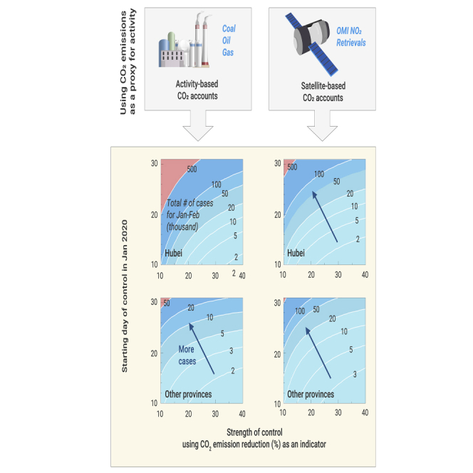
Dependence of the Number of COVID-19 Cases on the Strength of Interventions

Early action on 23 January was critical in limiting the number of COVID-19 cases in January–February 2020 to 81,106 cases, compared with our prediction of 79,000 cases as a central model estimate (45,300–137,700) with a bottom-up method or of 80,000 cases (46,700–135,500) with a top-down method under the actual scenario (Figure 6). If the interventions were taken after 24 January under the same emission reduction of 12% (bottom-up) or 23% (top-down) as the actual scenario, total COVID-19 cases in China in January–February 2020 would have exceeded 100,000. Many activities were constrained, but additional energy consumption rose from the production of medical equipment such as facial masks and ventilators.²⁰ If the interventions had been delayed by 1 week, enhancement of the strength of containment required to limit COVID-19 cases below 100,000 in January–February would have increased China's CO₂ emission reduction from 11% to 21% (as a difference between the two methods) to 26%–50% (Figures 6G and 6H), henceforth causing greater damage to the economy.

Figure 6.

Dependence of the Number of COVID-19 Cases on the Strength and Timing of Interventions

(A and B) Comparison of the simulated and observed numbers of COVID-19 cases in January–February 2020 based on an estimate of CO₂ emissions as an indicator for human activity with a bottom-up (A) or top-down (B) method. The number of cases is predicted by province, and the sum for all provinces is indicated by a red dot. (C–H) Prediction of the number of COVID-19 cases in January–February 2020 under a given starting day and the percentage of CO₂ emission reduction as an indicator of reduced human activity in Hubei (C and D), other provinces (E and F), and China (G and H). The actual starting day and percentage of CO₂ emission reduction are indicated by red pentagrams.

Economic Losses and Gains from Reducing Activities during the COVID-19 Pandemic

The social costs of CO₂ emissions are conventionally considered to stem from the economic damage caused by release of CO₂ into the atmosphere and the subsequent climate change.³⁴ We defined the public-health costs of CO₂ emissions during the COVID-19 pandemic as a sum of the health-care cost for cured cases and the mortality cost for fatal cases if activities and CO₂ emissions are maintained, which will cause an increase in the daily rate of COVID-19 cases following the relationship shown in Figure 4. It should be noted that these public-health costs only exist during the epidemic and disappear when the pandemic is terminated. We estimated the costs of health care and fatalities using a Monte Carlo approach (Materials and Methods).^35,36 The public-health costs of increased COVID-19 cases due to maintaining CO₂-emitting activities amount to $740 (95% CI, $400–$1,100) t CO₂⁻¹, per tonne of CO_2, on the first day of the Wuhan travel ban (23 January) with a top-down method, which decrease over time as the pandemic is contained (Figure 7A). These costs are lower with a bottom-up method ($600 [t CO₂]⁻¹ on 23 January), which predicted a lower sensitivity of the rate of new COVID-19 cases to the percentage of reduction in CO₂ emissions (Figure 4). These public-health costs would amount to $4.3 trillion–$5.0 trillion (when 1 trillion = 10¹²) under an artificial scenario maintaining CO₂ emissions to protect the economy, which drops to $27 billion–$28 billion under the actual scenario (Figure 7B). The cost curve becomes flatter when CO₂ emissions are further reduced, indicating a decline in the efficacy of the containment. We compared the public-health costs associated with a quintile of actual CO₂ emission reduction with the direct reduction in gross domestic product (GDP) (Figure 7C). The public-health costs associated with the first quintile of CO₂ emission reduction ($3.6 trillion–$4.0 trillion) are nearly 8-fold larger than the direct loss of GDP in the first quarter of 2020 relative to 2016–2019 ($450 billion). The public-health costs associated with the fourth quintile of CO₂ emission reduction ($50 billion–$60 billion) are less than one-fifth of the GDP loss. These results confirm that interventions, using CO₂ emissions as an indicator could have generated greater benefits than the economic loss in the short term.⁷

Figure 7.

Economic Costs and Benefits of Containment during the COVID-19 Pandemic

(A) Using an estimate of CO₂ emissions as an indicator for human activity in 2020 with a bottom-up (red) or top-down (blue) method, the marginal costs of health care for cured cases (dotted line) and of mortality for fatal cases (dashed line) in January–May are estimated when one additional tonne of CO₂ is emitted to show the impact of maintaining activity on a given day between 20 January and 29 February in each province. The average marginal costs in China are calculated as an average weighted by provincial CO₂ emissions (Materials and Methods).

(B) The total costs of health care and mortality in a set of artificial scenarios, where actual daily CO₂ emission reduction is multiplied by a constant value (e.g., 0 indicates no intervention, and 2 indicates interventions at a doubled strength) in January–May 2020.

(C) Comparison of the public-health costs associated with a quintile of the actual daily CO₂ emission reduction to the direct loss of GDP (Materials and Methods). The bar for 100%–120% indicates an artificial scenario with 20% more CO₂ emissions reduced than the actual scenario. To assess the uncertainty in our estimate, we ran 10,000 Monte Carlo simulations, of which the median is indicated as a central estimate (line or bar) and the 95% CI is indicated as the uncertainty (shaded area or error line).

Policy Implications

We perform a correlation analysis to confirm that the daily rate of new COVID-19 cases is lower when more activities and CO₂ emissions are contained in China as measured using both statistical data for energy consumption and satellite retrievals of NO₂ column concentration. These relationships lead to substantial public-health costs of maintaining activities and CO₂ emissions in the pandemic of COVID-19; avoiding these costs by the control policies in China creates substantial benefits 10-fold larger than the loss of GDP in the first quarter of 2020. The peak of the COVID-19 pandemic is likely higher in the winters of 2020 and 2021 than in 2019,³⁷ with a potential resurgence as far into the future as 2025,⁴ while the impact of COVID-19 will inevitably last for years or even decades.³⁸ Low oil prices and low interest rates during the pandemic are also likely to continue for years.³⁹ On the positive side, a rising social cost of CO₂ emissions would create an opportunity to decarbonize the energy system under a shrinking supply of carbon-emitting energy, an increasing demand for high-tech industries, and the pursuit of a lifestyle that consumes less energy. On the negative side, the expense of containing the pandemic consumes energy for medical equipment production²⁰ and competes for investments in renewable energy.⁴⁰ The pandemic caused a decline in CO₂ emissions in the first quarter of 2020, but these emissions will increase in the long term as the economy recovers and social activities are re-opened; if CO₂ emissions had been maintained during the pandemic, the emissions would be lower in the long term when the economy would collapse. The same could occur in the event of disastrous climate change.⁴¹ When considering the impact of COVID-19, an integrated approach is essential and urgently needed; public health can no longer be separated from either climate change or human society. Our study using a geographic method suggests an unprecedentedly high cost of maintaining activities and CO₂ emissions during the COVID-19 pandemic and confirms the effects of China's swift actions by saving human lives and substantial public health costs.

Materials and Methods

Daily Confirmed Local COVID-19 Cases in 30 Provinces

We constructed a dataset of daily local cases of COVID-19 by excluding the imported cases in China from 15 January to 31 May in 2020 in three steps. First, in the period from 12 March to 31 May, we compiled the imported and local cases of COVID-19 infection from the National Health Commission of the People's Republic of China (NHC) (http://www.nhc.gov.cn/xcs/xxgzbd/gzbd_index.shtml), which distinguished the local cases from the imported cases of COVID-19 on each day. Second, in the period from 1 March to 11 March, we compiled the total cases of COVID-19 infection from the NHC (http://www.nhc.gov.cn/xcs/xxgzbd/gzbd_index.shtml), without information on either imported or local cases. To identify the local cases, we compiled the imported cases of COVID-19 on each day released by the new crown epidemic daily analysis report (NCER) (https://datanews.caixin.com/interactive/2020/pneumonia-h5/#live-data). Third, in the period from 15 January to 29 February, the NHC and NCER released the local cases of COVID-19 in Hubei province. For other provinces, we compiled the local cases of COVID-19 from the Harvard dataset (https://dataverse.harvard.edu/dataverse/2019ncov). To estimate the relationship between the daily rate of new COVID-19 cases and CO₂ emission reduction, we analyzed the number of daily local cases after excluding these cases imported from regions out of China's mainland.

Monthly CO₂ Emissions by Province and Sector during 2016–2020

Because official statistical data for annual energy consumption in China has not yet been released for the years after 2017, and monthly energy consumption is not available, we needed the prediction of energy consumption by month from 2016 to 2020 to estimate the monthly CO₂ emissions as a bottom-up method. In two recent studies,^8,9 CO₂ emissions in 2020 were predicted by scaling the annual emissions in earlier years (most original data are obtained for 2017, and are extended to 2019 using preliminary or forecast data; see details in Friedlingstein et al.⁴²) with monthly sector-specified activity data to estimate CO₂ emissions globally. In these studies, the underlying assumption is that the ratio of emission rate to activity is a constant. Different from the scaling method,^8,9 we (1) developed 420 regression models between the annual energy consumption and the annual activity data over the 21 years of 1997–2017 in 14 economic and production sectors (listed in Table S2) in 30 provinces (a total of 14 × 30 = 420 regression models, of which the original data are given in Data S1); and (2) predicted the monthly energy consumption in January–May over 2016–2020 based on the monthly activity data in January–May of 2016–2020 using these 420 regression models. To compile the annual data for energy consumption and activities over the 21 years of 1997–2017, we selected 30 provinces in China by excluding Tibet, Hong Kong, Macau, and Taiwan due to lack of data. The procedures for compiling energy data are provided in the Supplemental Methods. Based on energy consumption in the 15 sectors (one sector is the remaining sectors other than the 14 sectors in Table S2) and cement production over 2016–2020, monthly bottom-up CO₂ emission (E_mt) was estimated as:

$$E_{mt}^{original}=\sum _{h=1}^{30}{E}_{mth}^{original}=\sum _{h=1}^{30}\sum _{s=1}^{16}{E}_{mths}^{original}=\sum _{h=1}^{30}\sum _{s=1}^{16}\sum _{q=1}^3\left(J_{mths}{f}_{mthsq}{e}_q{g}_q\right)$$ (Equation 3)

where m is a month, t is a year, h is a province, s is a sector, q is a type of fuel (1–3 for coal, oil, and gas, respectively), J_mths is the energy consumed or cement produced, f_mthsq is the fraction of energy q in energy consumption as an average for 2016–2017 based on the energy data released by the National Bureau of Statistics of China (1 for cement production),⁴³ e_q is the emission factor, and g_q is the oxygenation efficiency (1 for cement production). To estimate emissions, we applied an emission factor of 96.6 t CO₂ (TJ coal)⁻¹, 69.4–77.4 t CO₂ (TJ oil)⁻¹, 56.2–78.9 t CO₂ (TJ gas)⁻¹ and 0.2916 t CO₂ (t cement production)⁻¹, and oxygenation efficiency of 74%–90% for coal, 96% for oil, and 91%–98% for gas.⁴⁴ The estimated monthly CO₂ emissions over 2016–2020 in 30 provinces are provided in Data S2.

To show the impact of COVID-19 on CO₂ emissions in 2020, the estimated CO₂ emissions were detrended by removing a temporal trend over 2016–2019 that best fits the data in the least squares sense (https://ww2.mathworks.cn/help/ident/ref/detrend.html) as:

$$E_{mths}^{detrended}=E_{mths}^{original}+{\phi }_{mhs}\cdot \left(2020-t\right)$$ (Equation 4)

where t is a year, and φ_mhs is the linear regression slope of $E_{mths}^{original}$ against year t.

A Dataset of Satellite-Based NO₂ Column Concentration Corrected for the Annual Trends and Impacts of Meteorology

We compiled a dataset of daily NO₂ column concentration at a resolution of 0.25° × 0.25° from satellite retrievals and nine meteorological variables from global re-analysis data (see detailed sources of data in the Supplemental Methods). To identify the impact of COVID-19, we corrected for inter-annual trends and the impact of meteorological changes in the temporal trend of NO₂ column concentration in three steps. First, log₁₀-transformed NO₂ column concentration was detrended by removing inter-annual trends over 2016–2019 that best fit the data in the least squares sense (https://ww2.mathworks.cn/help/ident/ref/detrend.html) as:

$$lo{g}_{10}{C}_{ijt}^{detrended}=lo{g}_{10}{C}_{ijt}^{original}+{\varphi }_i\cdot \left(2020-t\right)$$ (Equation 5)

where i is a grid, j is a day, t is a year, $C_{ijt}^{original}$is NO₂ column concentration retrieved from the satellite, and ϕ_i is the coefficient in the regression of the log₁₀-transformed NO₂ column concentration against the year t.

Second, for each grid, the detrended log₁₀-transformed NO₂ column concentration was regressed against the detrended meteorological variables (M_j,itk, k = 1 to 9 for temperature, pressure, relative humidity, wind speed, zonal wind, meridional wind, atmospheric precipitable water content, boundary layer height, and ozone column concentration). Correlation coefficients between $lo{g}_{10}{C}_{ijt}^{detrended}$ and daily meteorological variables are mapped in Figure S2. Given the correlation between $lo{g}_{10}{C}_{ijt}^{detrended}$and daily meteorological variables, we adopted a partial-least-square regression using a lag model as:⁴⁵

$$lo{g}_{10}{C}_{ijt}^{detrended}=\sum _{\tau =0}^3\sum _{k=1}^9\left(c_{\tau ,ik}\cdot M_{j-\tau ,itk}\right)+b_i⋮$$ (Equation 6)

where i is a grid, j is a day, t is a year, k denotes one meteorological variable, τ is the lag day in the effect of meteorology on concentration (e.g., τ = 3 denotes the meteorological variables on 3 days before day i), c_τ,ik is a regression coefficient, and b_i is a constant.

Third, log₁₀-transformed NO₂ concentration corrected for the impact of meteorology (C_ijt) can be derived as:

$$lo{g}_{10}{C}_{ijt}=lo{g}_{10}{C}_{ijt}^{detrended}+\sum _{\tau =0}^3\sum _{k=1}^9{c}_{\tau ,ik}\cdot \left({\overline{M}}_k-M_{j-\tau ,itk}\right)$$ (Equation 7)

where ${\overline{M}}_k$ is the average meteorology over January–May in 2020. The NO₂ column concentration is log₁₀ transformed to consider a first-order change in atmospheric physical and chemical processes.⁴⁶ For each province, we calculated an average NO₂ column concentration (C_hjt, where h is a province) weighted by gridded CO₂ emissions (see detailed procedures in the Supplemental Methods).

Estimation of Daily CO₂ Emissions by a Bottom-Up Method

Because the first state-level action of the Wuhan travel ban was released on 23 January, we assumed that COVID-19 did not contribute considerably to changes in CO₂ emissions in December between 2015–2018 and 2019, which serves as a reference change in the absence of COVID-19. We took the average of daily CO₂ emissions over 2016–2019 as a reference, rather than a specific day. We estimated daily CO₂ emissions on a day in 2020 based on the change in concentration, measured as the CCF (Equation 2). We estimated changes in daily CO₂ emissions with COVID-19 relative to a reference without COVID-19 as:

$$\Delta E_{jh}=E_{jh}-E_{0jh}=E_{mh,2020}\cdot \frac{CC{F}_{hj}}{{\sum }_{j=1}^{n_m}CC{F}_{hj}}-\frac{\overline{E_{mh,2016-2019}}}{n_m}\cdot \frac{E_{0h,2019}}{\overline{E_{0h,2015-2018}}}$$ (Equation 8)

where j is a day, h is a province, m is a month, and n_m is the number of days in month m. E_jh and E_0jh are daily CO₂ emissions with and without COVID-19, respectively. E_mh,2020 and $\overline{E_{mh,2016-2019}}$are the monthly detrended CO₂ emissions in 2020 and the monthly detrended average for 2016–2019, respectively. $E_{0h,2019}$and $\overline{E_{0h,2015-2018}}$are the detrended CO₂ emissions in December 2019 and the detrended average for December 2015–2018, respectively.

Estimation of Daily CO₂ Emissions by a Top-Down Method

We used a top-down method to estimate the change in CO₂ emissions due to COVID-19 based on satellite retrievals of NO₂ column concentration. We assumed that COVID-19 did not contribute considerably to changes in NO₂ column concentration in December between 2015–2018 and 2019, which serves as a reference change in the absence of COVID-19. We estimated changes in daily CO₂ emissions with COVID-19 relative to a reference without COVID-19 as:

$$\Delta E_{jh}=E_{jh}-E_{0jh}=E_{0jh}\cdot CC{F}_{hj}-E_{0jh}=\frac{\overline{E_{mh,2016-2019}}}{n_m}\cdot \frac{\overline{E_{0h,2019}}}{\overline{E_{0h,2015-2018}}}\cdot \left(CC{F}_{hj}-1\right)$$ (Equation 9)

where j is a day, h is a province, and m is a month. E_jh and E_0jh are the daily CO₂ emission rates with and without COVID-19, respectively. $\overline{E_{mh,2016-2019}}$is the monthly detrended CO₂ emissions as an average for 2016–2019. $E_{0h,2019}$and $\overline{E_{0h,2015-2018}}$are the detrended CO₂ emissions in December 2019 and the detrended average for December 2015–2018, respectively. CCF_hj denotes the concentration change on a given day relative to an average of the same days in 2016–2019, which is calculated by Equation 2.

Relationship of the Epidemic to Daily CO₂ Emissions

To simulate the daily evolution of new COVID-19 cases by province, we developed a regression model between the percentage of CO₂ emission reduction to emissions in January–May and the daily rate of new cases as:

$$V_{j,h}=B_h+S_h\cdot {\Lambda }_{j,h}$$ (Equation 10)

where j is a day, h is a province, V_j,h is the daily rate of local new cases, Λ_j,h is total CO₂ emission reduction as a percentage of CO₂ emissions in January–May (see Equation 11), S_h is the slope of the regression, and B_h is the intercept of the regression. Provincial S_h and B_h are listed in Table S3. Λ_j,h was calculated as:

$${\Lambda }_{j,h}=\frac{\Delta TE{R}_{jh}}{TE{R}_{0h}}=\frac{{\sum }_{d=1}^j\Delta E_{dh}}{{\sum }_{d=1}^{152}{E}_{0dh}}=\frac{{\sum }_{d=1}^j\left(E_{dh}-E_{0dh}\right)}{{\sum }_{d=1}^{152}{E}_{0dh}}$$ (Equation 11)

where d is a day, and 152 denotes the last day (d) for 31 May 2020 (d = 1 for 1 January 2020). ΔTER_jh is total CO₂ emission reduction due to COVID-19. TER_0h is total CO₂ emissions in January–May without COVID-19. ΔE_dh is change in daily CO₂ emissions due to COVID-19. E_dh and E_0dh are daily CO₂ emissions with or without COVID-19, respectively (Equations 8 and 9).

For each province, the number of daily new COVID-19 cases (N) was predicted as:

$$N_{j+1,h}=N_{j,h}\cdot exp\left(V_{j+1,h}\right)$$ (Equation 12)

where j is a day. To initialize the simulation, we obtained the initial number of daily cases (N_0,h) as that from the fourth day after the first infection was reported in a province, which was estimated as the average number of daily cases during the three adjacent days with reported cases.

In Figures 5 and 6, we simulated the spread of COVID-19 under a varying starting day and percentage of emission reduction by modifying Equation 10 into:

$$V_{j,h}=B_h+S_h\cdot {\Lambda }_{j+n,h}\cdot \frac{\mu }{{\Lambda }_{152,h}}$$ (Equation 13)

where n denotes the change of the start day of interventions (n is positive to denote a delay and negative to show earlier interventions, while n is shown by the vertical axis in Figures 6C–6F), Λ_152,h is the actual percentage of emission reduction in January–May (152 denotes 31 May 2020), and μ is the tested percentage of emission reduction in January–May (μ is zero for no interventions, while μ is shown by the horizontal axis in Figures 6C–6F).

Estimation of Economic Values

We estimated the public-health costs of CO₂ emissions by considering costs of health care for cured cases and mortality costs for fatal cases during the COVID-19 pandemic. Given the difference in the costs of a cured or fatal case, we divided the population of COVID-19 cases into nine age groups (0–9, 10–19, 20–29, 30–39, 40–49, 50–59, 60–69, 70–79, and ≥80 years old). We calculated the public-health costs in January–May 2020 for each province as:

$$T_h=\sum _{d=1}^{152}d{N}_{dh}\cdot \left(c{c}_h\cdot \sum _{\eta =1}^9{\sigma }_{\eta }\cdot {\Phi }_{cc,\eta }+f{c}_h\cdot \sum _{\eta =1}^9{\delta }_{\eta }\cdot {\Phi }_{fc,\eta }\right)$$ (Equation 14)

where h is a province, d is a day, η is an age group, 152 denotes 31 May 2020, N_hd is the number of daily new cases, cc_h or fc_h is the fraction of cured or fatal cases during COVID-19 in each province,⁴⁷ σ_η or δ_η is the fraction of age group η in the confirmed or fatal cases,⁴⁸ Φ_cc,η is the unit cost in the course of infection for a cured case,³⁵ and Φ_fc,η is the unit cost in the course of infection for a fatal case.³⁶ To estimate the costs of cured or fatal cases due to maintenance of CO₂-emitting activities, we designed a set of artificial scenarios of CO₂ emissions, which are detailed in the Supplemental Methods.

In addition to the public-health costs, the loss of GDP was estimated. We used an empirical method to estimate the loss of GDP in the first quarter of 2020 based on a linear regression of GDP in the first quarter over 2016–2019 against years (GDP = 1,871.3t−3,756,238.3, where t is the year).⁴⁹ The difference between the predicted GDP in 2020 (23,787.7 billion CNY or US$3,383.7 billion) and the observed value in 2020 (206,504.3 billion CNY or US$2,937.5 billion) was considered as the direct loss of GDP due to the COVID-19 pandemic (3,383.7−2,937.5 = US$446.2 billion) (shown as the purple bar in Figure 7C). The quarterly data for GDP for 2016–2020 in 30 provinces in China were compiled from the statistics of the National Bureau of Statistics of China (NBSC) (https://datanews.caixin.com/interactive/2020/pneumonia-h5/#live-data).

Uncertainty Analyses: Monte Carlo Simulations

To assess the uncertainty in the simulation of COVID-19 spread and the costs of health care and fatalities, we ran 10,000 Monte Carlo simulations where the following parameters were varied randomly: (1) the coefficients in the regression of the daily rate of new cases against CO₂ emission reduction, of which 95% CIs were applied (see the ranges in Figure 4); (2) the number of new cases on the day with the first case confirmed with 2019-nCoV, which was taken from a normal distribution with the average and standard deviation of the numbers over the first 7 days; and (3) the costs in the course of infection for a cured or fatal case (the 95% CIs are listed in Table S5). We adopted random values for these parameters from their normal distributions in Monte Carlo simulations. We used the median to indicate the central estimate and used the 95% CI to indicate the uncertainty range.

Published: November 25, 2020

Lead Contact Website

http://homepage.fudan.edu.cn/rongwang/en.

References

- 1.The State Council Information Office of the People's Republic of China Fighting Covid-19 China in Action. 2020. http://www.scio.gov.cn/ztk/dtzt/42313/43142/index.htm
- 2.World Health Organization (WHO) Report of the WHO–China Joint Mission on Coronavirus Disease 2019 (COVID-19) 2020. https://www.who.int/publications-detail/report-of-the-who-china-joint-mission-on-coronavirus-disease-2019-(covid-19)
- 3.Wang X., Zhang R.H. How does air pollution change during COVID-19 outbreak in China? Bull. Amer. Meteorol. Soc. 2020 doi: 10.1175/BAMS-D-20-0102.1. [DOI] [Google Scholar]
- 4.Kissler S.M., Tedijanto C., Goldstein E., et al. Projecting the transmission dynamics of SARS-CoV-2 through the postpandemic period. Science. 2020;368:860–868. doi: 10.1126/science.abb5793. [DOI] [PMC free article] [PubMed] [Google Scholar]
- 5.Kraemer M.U.G., Yang C.H., Gutierrez B., et al. The effect of human mobility and control measures on the COVID-19 epidemic in China. Science. 2020;368:493–497. doi: 10.1126/science.abb4218. [DOI] [PMC free article] [PubMed] [Google Scholar]
- 6.Tian H.Y., Liu Y.H., Li Y.D., et al. An investigation of transmission control measures during the first 50 days of the COVID-19 epidemic in China. Science. 2020;368:638–642. doi: 10.1126/science.abb6105. [DOI] [PMC free article] [PubMed] [Google Scholar]
- 7.Wu Z.Y., McGoogan J.M. Characteristics of and important lessons from the coronavirus disease 2019 (COVID-19) outbreak in China: summary of a report of 72 314 cases from the Chinese Center for Disease Control and Prevention. JAMA. 2020;323:1239–1242. doi: 10.1001/jama.2020.2648. [DOI] [PubMed] [Google Scholar]
- 8.Le Quéré C., Jackson R.B., Jones M.W., et al. Temporary reduction in daily global CO2 emissions during the COVID-19 forced confinement. Nat. Clim. Change. 2020;10:647–653. [Google Scholar]
- 9.Liu Z., Deng Z., Ciais P., et al. COVID-19 causes record decline in global CO2 emissions. arXiv. 2020 https://arxiv.org/abs/2004.13614 [Google Scholar]
- 10.Zhang R.X., Zhang Y., Lin H., et al. NOx emission reduction and recovery during COVID-19 in East China. Atmosphere. 2020;11:433. [Google Scholar]
- 11.Zheng B., Geng G., Ciais P., et al. Satellite-based estimates of decline and rebound in China’s CO2 emissions during COVID-19 pandemic. arXiv. 2020 doi: 10.1126/sciadv.abd4998. https://arxiv.org/abs/2006.08196 [DOI] [PMC free article] [PubMed] [Google Scholar]
- 12.Konovalov I.B., Berezin E.V., Ciais P., et al. Estimation of fossil-fuel CO2 emissions using satellite measurements of “proxy” species. Atmos. Chem. Phys. 2016;16:13509–13540. [Google Scholar]
- 13.Goldberg D.L., Anenberg S.C., Griffin D., et al. Disentangling the impact of the COVID-19 lockdowns on urban NO2 from natural variability. Geophy. Res. Lett. 2020 doi: 10.1029/2020GL089269. [DOI] [PMC free article] [PubMed] [Google Scholar]
- 14.Berenzin E.V., Konovalov I.B., Ciais P., et al. Multiannual changes of CO2 emissions in China: indirect estimates derived from satellite measurements of tropospheric NO2 columns. Atmos. Chem. Phys. 2013;13:9415–9438. [Google Scholar]
- 15.Goldberg D.L., Lu Z.F., Oda T., et al. Exploiting OMI NO2 satellite observations to infer fossil-fuel CO2 emissions from US megacities. Sci. Total Environ. 2019;695:133805. doi: 10.1016/j.scitotenv.2019.133805. [DOI] [PubMed] [Google Scholar]
- 16.Akimoto H., Ohara T., Kurokawa J., Horii N. Verification of energy consumption in China during 1996–2003 by using satellite observational data. Atmos. Environ. 2006;40:7663–7667. [Google Scholar]
- 17.Russell A.R., Valin L.C., Cohen R.C. Trends in OMI NO2 observations over the United States: effects of emission control technology and the economic recession. Atmos. Chem. Phys. 2012;12:12197–12209. [Google Scholar]
- 18.Liu F., Page A., Strode S.A., et al. Abrupt decline in tropospheric nitrogen dioxide over China after the outbreak of COVID-19. Sci. Adv. 2020;6:eabc2992. doi: 10.1126/sciadv.abc2992. [DOI] [PMC free article] [PubMed] [Google Scholar]
- 19.Bauwens M., Compernolle S., Stavrakou T., et al. Impact of coronavirus outbreak on NO2 pollution assessed using TROPOMI and OMI observations. Geophy. Res. Lett. 2020;47 doi: 10.1029/2020GL087978. e2020GL087978. [DOI] [PMC free article] [PubMed] [Google Scholar]
- 20.Livingston E., Desai A., Berkwits M. Sourcing personal protective equipment during the COVID-19 pandemic. JAMA. 2020;323:1912–1914. doi: 10.1001/jama.2020.5317. [DOI] [PubMed] [Google Scholar]
- 21.Krotkov N.A., Lamsal L.N., Celarier E.A., et al. The version 3 OMI NO2 standard product. Atmos. Meas. Tech. 2017;10:3133–3149. [Google Scholar]
- 22.Laughner J.L., Cohen R.C. Direct observation of changing NOx lifetime in North American cities. Science. 2019;366:723–727. doi: 10.1126/science.aax6832. [DOI] [PMC free article] [PubMed] [Google Scholar]
- 23.Wang R., Saunders H., Moreno-Cruz J., Caldeira K. Induced energy-saving efficiency improvements amplify effectiveness of climate change mitigation. Joule. 2019;3:2103–2119. [Google Scholar]
- 24.Zhao S.L., Chen H. Modeling the epidemic dynamics and control of COVID-19 outbreak in China. Quant. Biol. 2020;8:11–19. doi: 10.1007/s40484-020-0199-0. [DOI] [PMC free article] [PubMed] [Google Scholar]
- 25.Oda T., Maksyutov S., Andres R.J. The Open-source Data Inventory for Anthropogenic Carbon dioxide (CO2), version 2016 (ODIAC2016): a global, monthly fossil-fuel CO2 gridded emission data product for tracer transport simulations and surface flux inversions. Earth Syst. Sci. Data. 2018;10:87–107. doi: 10.5194/essd-10-87-2018. [DOI] [PMC free article] [PubMed] [Google Scholar]
- 26.Cheng K.K., Lam T.H., Leung C.C. Wearing face masks in the community during the COVID-19 pandemic: altruism and solidarity. Lancet. 2020 doi: 10.1016/S0140-6736(20)30918-1. [DOI] [PMC free article] [PubMed] [Google Scholar]
- 27.Block P., Hoffman M., Raabe I.J., et al. Social network-based distancing strategies to flatten the COVID-19 curve in a post-lockdown world. Nat. Hum. Behav. 2020;4:588–596. doi: 10.1038/s41562-020-0898-6. [DOI] [PubMed] [Google Scholar]
- 28.Stein-Zamir C., Abramson N., Shoob H., et al. A large COVID-19 outbreak in a high school 10 days after schools’ reopening, Israel, May 2020. Euro. Surveill. 2020;25:2001352. doi: 10.2807/1560-7917.ES.2020.25.29.2001352. [DOI] [PMC free article] [PubMed] [Google Scholar]
- 29.Kendall M., Milsom L., Abeler-Dorner L., et al. COVID-19 incidence and R decreased on the Isle of Wight after the launch of the test, trace, isolate programme. medRxiv. 2020 doi: 10.1101/2020.07.12.20151753. [DOI] [PMC free article] [PubMed] [Google Scholar]
- 30.Hao X.J., Cheng S.S., Wu D.G., et al. Reconstruction of the full transmission dynamics of COVID-19 in Wuhan. Nature. 2020;584:420–424. doi: 10.1038/s41586-020-2554-8. [DOI] [PubMed] [Google Scholar]
- 31.Jia X., Chen J., Li L., et al. Modeling the prevalence of asymptomatic COVID-19 infections in the Chinese mainland. The Innovation. 2020;1:100026. doi: 10.1016/j.xinn.2020.100026. [DOI] [PMC free article] [PubMed] [Google Scholar]
- 32.Althouse B.M., Wallace B., Case B., et al. The unintended consequences of inconsistent pandemic control policies. arXiv. 2020 https://arxiv.org/abs/2008.09629 [Google Scholar]
- 33.Zhang J.J., Litvinova M., Wang W., et al. Evolving epidemiology and transmission dynamics of coronavirus disease 2019 outside Hubei province, China: a descriptive and modelling study. Lancet Infect. Dis. 2020;20:793–802. doi: 10.1016/S1473-3099(20)30230-9. [DOI] [PMC free article] [PubMed] [Google Scholar]
- 34.Nordhaus W.D. An optimal transition path for controlling greenhouse gases. Science. 1992;258:1315–1319. doi: 10.1126/science.258.5086.1315. [DOI] [PubMed] [Google Scholar]
- 35.Bartsch S.M., Ferguson M.C., McKinnell J.A., et al. The potential health care costs and resource use associated with COVID-19 in the United States. Health Aff. 2020;39:927–935. doi: 10.1377/hlthaff.2020.00426. [DOI] [PMC free article] [PubMed] [Google Scholar]
- 36.Thunström L., Newbold S.C., Finnoff D., et al. The benefits and costs of using social distancing to flatten the curve for COVID-19. J. Benefit Cost Anal. 2020;11:179–195. [Google Scholar]
- 37.Neher R.A., Dyrdak R., Druelle V., et al. Potential impact of seasonal forcing on a SARS-CoV-2 pandemic. Swiss Med. Wkly. 2020;150:w20224. doi: 10.4414/smw.2020.20224. [DOI] [PubMed] [Google Scholar]
- 38.McKibbin W.J., Fernando R. The Glob. macroeconomic impacts COVID-19: Seven scenarios. CAMA Working Paper No. 19/2020. 2020. [DOI]
- 39.Steffen B., Egli F., Pahle M., Schmidt T.S. Navigating the clean energy transition in the COVID-19 crisis. Joule. 2020;4:1137–1141. doi: 10.1016/j.joule.2020.04.011. [DOI] [PMC free article] [PubMed] [Google Scholar]
- 40.Gillingham K.T., Knittel C.R., Li J., et al. The short-run and long-run effects of Covid-19 on energy and the environment. Joule. 2020;4:1337–1341. doi: 10.1016/j.joule.2020.06.010. [DOI] [PMC free article] [PubMed] [Google Scholar]
- 41.Woodard D.L., Davis S.J., Randerson J.T. Economic carbon cycle feedbacks may offset additional warming from natural feedbacks. Proc. Natl. Acad. Sci. U S A. 2019;116:759–764. doi: 10.1073/pnas.1805187115. [DOI] [PMC free article] [PubMed] [Google Scholar]
- 42.Friedlingstein P., Jones M., O'sullivan M., et al. Global carbon budget 2019. Earth Syst. Sci. Data. 2019;11:1783–1838. [Google Scholar]
- 43.National Bureau of Statistics of China (NBSC) China Energy Statistics Yearbook. 2018. http://www.stats.gov.cn/english/Statisticaldata/AnnualData/
- 44.Shan Y.L., Huang Q., Guan D.B., Hubacek K. China CO2 emission accounts 2016-2017. Sci. Data. 2020;7:1–9. doi: 10.1038/s41597-020-0393-y. [DOI] [PMC free article] [PubMed] [Google Scholar]
- 45.Brown P.T., Caldeira K. Greater future global warming inferred from Earth’s recent energy budget. Nature. 2017;552:45–50. doi: 10.1038/nature24672. [DOI] [PubMed] [Google Scholar]
- 46.Wang R., Tao S., Wang B., et al. Sources and pathways of polycyclic aromatic hydrocarbons transported to Alert, the Canadian High Arctic. Environ. Sci. Technol. 2010;44:1017–1022. doi: 10.1021/es902203w. [DOI] [PubMed] [Google Scholar]
- 47.Report of Real Time Data of COVID-19 (RRTD). (2020), https://voice.baidu.com/act/newpneumonia/newpneumonia/?from=osari_pc_3.
- 48.Novel C.P.E.R.E. The epidemiological characteristics of an outbreak of 2019 novel coronavirus diseases (COVID-19) — China, 2020. China CDC Weekly. 2020;2:113–122. [PMC free article] [PubMed] [Google Scholar]
- 49.Burke M., Hsiang S.M., Miguel E. Global non-linear effect of temperature on economic production. Nature. 2015;527:235–239. doi: 10.1038/nature15725. [DOI] [PubMed] [Google Scholar]
Associated Data
This section collects any data citations, data availability statements, or supplementary materials included in this article.