Effect of Inter-layer Coupling on Multilayer Network Centrality Measures

Abstract

The study of networks has been evolving because of its applications in diverse fields. Many complex systems involve multiple types of interactions and such systems are better modeled as multilayer networks.The question “which are the most (or least) important nodes in a given network?”, has gained substantial attention in the network science community. The importance of a node is known as centrality and there are multiple ways to define it. Extending the centrality measure to multilayer networks is challenging since the relative contribution of intra-layer edges vs. that of inter-layer edges to multilayer centrality is not straight-forward. With the growing applications of multilayer networks, several attempts have been made to define centrality in multilayer networks in recent years. There are different ways of tuning the inter-layer couplings which may lead to different classes of centrality measures. In this article, we provide an overview of the recent works related to centrality in multilayer networks with a focus on key use cases and implications of the type of inter-layer coupling on centrality and subsequent uses of the different centrality measures. We discuss the effect of three popular interlayer coupling methods viz. diagonal coupling between adjacent layers, diagonal coupling and cross coupling. We hope the colloquial tone of this article would make it a pleasant read for understanding the theoretical as well as experimental aspects of the work.

1. Introduction

Many real-world complex systems can be modeled as networks. The interacting agents of the system are represented by nodes and interactions among them are represented by a set of edges. Study of networks is profoundly an interdisciplinary area and has different sets of problems in different domains. The importance of a node in the network, also known as the node centrality, has applications in several domains such as finding the most influential people in social networks, essential genes/proteins in biological networks, crucial infrastructures in transportation networks and hubs of information in information networks. Similar to node centrality, we can also find important edges or other structures (such as sub-networks) in the network^{12, 24, 39}. We focus on node centrality (hereafter referred to as centrality) in this work.

Centrality can be defined in multiple ways depending on the type of a network (directed/ undirected, size) or application domain. For example, PageRank is an appropriate centrality measure for ranking the web pages in response to a search query¹⁷, whereas betweenness centrality is useful for designing the packet routing strategies in computer networks¹⁴. In this section, we will introduce this term. We will not provide a thorough study of centrality measures for monoplex (i.e., single layer) networks, which can be found at³². Let A ∈ ℝ^{N × N} be the adjacency matrix of a monoplex network with N nodes, where A_ij is the strength of the ij ^th connection. Let x ∈ R ^N be the centrality vector of a network where x_i represents the centrality of node i. For a given adjacency matrix A, the corresponding centrality vector x can be calculated in the ways mentioned in Table 1. With the advent of data collection methods and superior data processing techniques, many times we have access to multiple views of the data. For example, a set of authors can have multiple types of relationships among them such as co-authorship, citation, co-citation, etc. Networks that change their structure with time can also give rise to multiple data views. In such cases, each view corresponds to the network structure at one particular time stamp. Such networks are known as temporal networks and they can be modeled by multilayer networks. Multilayer networks have found immense applications in ecological systems³⁶, biological systems¹⁹, transport systems², social network analysis⁴⁹, etc. With the abundance of applications in several domains, multilayer networks are known by different terminologies such as multiplex networks, interconnected networks, multidimensional networks, etc.²⁷. The key difference between a multilayer network and a set of monoplex (single layer) networks is the presence of inter-layer edges in the former.

Table 1.

Centrality measures for monoplex networks. For detailed description of these measures and many others, please refer³²

Centrality measure	Centrality of node i	Description
Eigenvector centrality	$$x_i={\lambda }^{-1}j{A}_{ij}{x}_j$$	λ is the leading eigenvalue
PageRank centrality	$$x_i=\alpha j{A}_{ij}\frac{x_j}{k_j}$$	α is a scalar and kj is the degree of node j
HITS centrality (authority)	$$x_i=\alpha j{A}_{ij}{y}_j$$	α is a scalar and yj is the hub centrality of node j
HITS centrality (hub)	$$y_i=\alpha j{A}_{ij}{x}_j$$	α is a scalar and xj is the authority centrality of node j
Betweenness centrality	$$x_i=st\frac{n_{\text{st}}^i}{g_{\text{st}}}$$	ni st is the # of shortest paths between sandt that go through i. gst is the total # of shortest paths between nodes sand t

Finding centrality in multilayer networks has immense applications such as the study of the emergence of congestion in transport flows⁴⁵, ranking in evolving networks²⁹, and analyzing different life stages in the species⁴¹. In multilayer networks, the local neighborhood of a node can comprise nodes from the same layer as well as nodes from other layers. To define a centrality measure for multilayer networks, one has to come up with a way to handle the multilayer neighborhood of a node. Recently there have been several attempts at defining centrality measures for multilayer networks. Most of these methods differ in the way they handle inter-layer coupling. For instance, the multiple layers can be merged to form a monoplex network, or at the other extreme, the multilayer network itself can be treated as a giant monoplex network. The coupling methods have their own implications when combined with the centrality measures. Despite the availability of several multilayer centrality measures, there is a lack of study on the applicability of these methods. In this work, we review the effect of inter-layer coupling on different centrality measures, and discuss their use cases.

In this article, we do not cover the entire spectrum of centrality measures but focus only on the study of different inter-layer coupling methods and their effect on the prominent centrality measures. Related reviews exist in the literature on multilayer networks in general^{3, 6, 25, 53}, and centrality measures in particular^{10, 21}. However, these works largely survey the centrality measures for only one particular kind of inter-layer coupling. Our work attempts to cover the centrality works involving different types of inter-layer coupling.

2. Mathematical Notations

Different centrality measures require the multilayer network to be represented in different formats and we represent two popular ways of representing a multilayer network here.

2.1. Supra-Adjacency List Representation

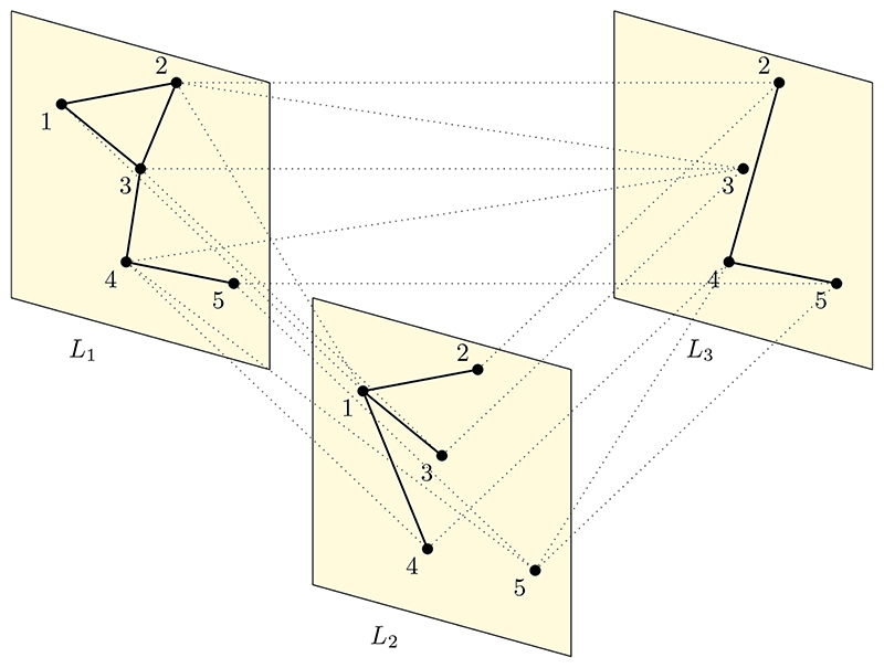
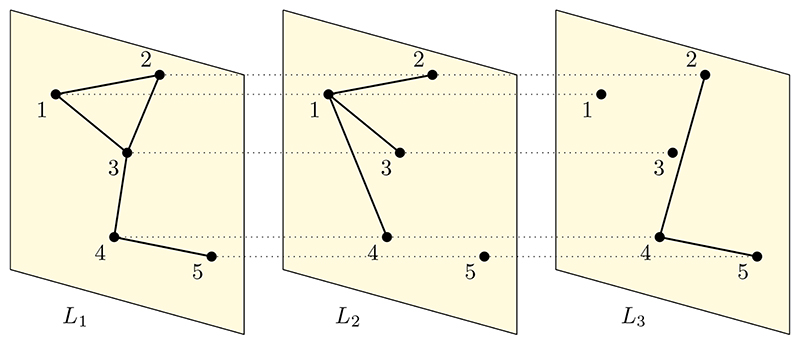
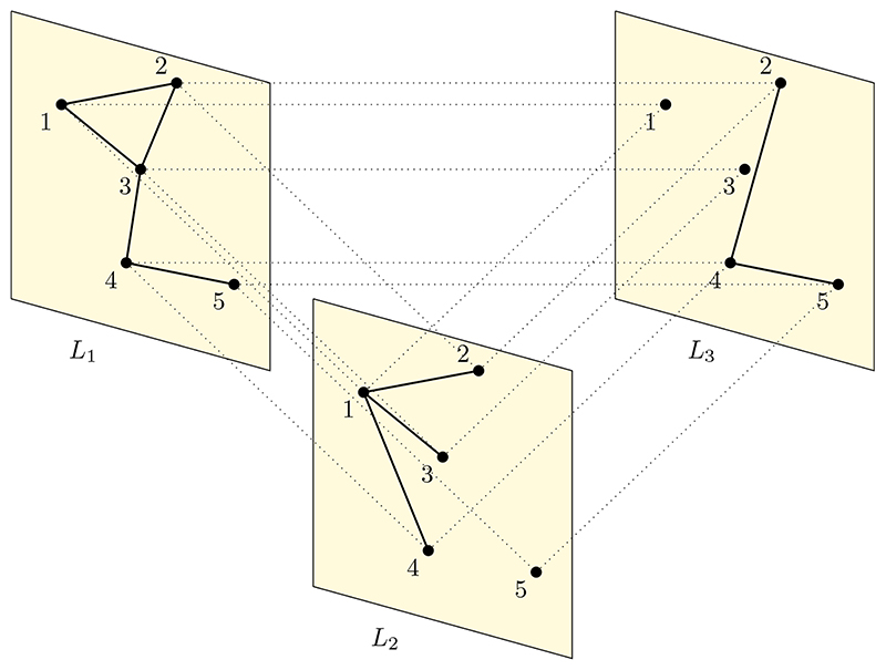
We represent a graph by G = (V, E), where V is a finite set of nodes with | V |= N and E is a set of node–node pairs representing the edges; E ⊆ V × V. Let L be the number of layers present in the multilayer network. As defined in²¹, let V_M ⊆ V × L represents the node–layer pairs such that (v, l) ∈ V_M if and only if v is present in layer l. The edge set spanning both within and across layers can be represented by E_M ⊆ V_M × V_M. A multilayer network can be represented by a quadruplet M = (V_M, E_M, V, L). For example, the multilayer network M shown in Fig. 1 has V ={1, 2, 3, 4, 5} and three layers L ={L₁, L₂, L₃}. The set of node–layer pairs can be represented as: V_M ={(1, L₁), (2,L₁), (3, L₁),(4, L₁), (5, L₁), (1,L₂),(2,L₂),(3,L₂),(4,L₂),(5,L₂),(2,L₃),(3,L₃), (4, L₃), (5, L₃)} V × L. The set of edges (intra-layer and inter-layer) can be represented as: EM = {{(1,L₁),(2,L₁)}, {(1,L₁),(3,L₁)}, {(2, L₁), (3, L₁)}, {(3,L₁),(4,L₁)}, {(4,L₁),(5,L₁)}, {(1, L₂), (2, L₂)}, {(1,L₂),(3,L₂)}, {(1,L₂),(4,L₂)}, {(2, L₃), (4, L₃)}, {(4,L₃),(5,L₃)}, {(1,L₁),(1,L₂)}, {(2, L₁), (1, L₂)}, {(3,L₁),(3,L₂)}, {(4,L₁),(4,L₂)}, {(4, L₁), (5, L₂)}, {(5,L₁),(5,L₂)}, {(2,L₁),(2,L₃)}, {(2, L₁), (3, L₃)}, {(3,L₁),(3,L₃)}, {(4,L₁),(3,L₃)}, {(5, L₁), (5, L₃)}, {(2,L₂),(2,L₃)}, {(3,L₂),(3,L₃)}, {(4, L₂), (4, L₃)}, {(5, L₂), (4, L₃)}, {(5, L₂), (5, L₃)}}.

Figure 1. A multilayer network depicting the cross inter-layer coupling.

A node is allowed to have as many connections with nodes within the layer and nodes from other layers. The node set in the layers need not be the same among all layers, as node 1 is missing in L ₃.

2.2. Supra-Adjacency Matrix Representation

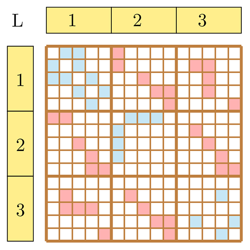
Following the convention used in¹⁸, we can flatten the multilayer network to a 2-dimensional supra-adjacency matrix. This is a special kind of matrix which has an inherent block structure. For the multilayer network shown in Fig. 1, the supra-adjacency matrix is shown in Fig. 2. Supraadjacency is an NL × NL dimensional matrix with diagonal blocks dedicated to intra-layer edges and non-diagonal blocks dedicated to interlayer edges. Presence of intra-layer edges is indicated by □ and inter-layer edges is indicated by □. Since all the edges (inter-layer and intra-layer) are undirected for this example, so the supraadjacency matrix is symmetric.

Figure 2. Supra-adjacency matrix representation M of the multilayer network shown in Fig. 1.

3. Inter-Layer Coupling Methods

There are different potential approaches for dealing with multiple layers and inter-layer edges of multilayer networks. The first approach is to ignore the layered structure of the network and treat nodes from all the layers like a giant network. One can use existing centrality measures on this entire network. This approach fails to distinguish between intra-layer and inter-layer edges, and hence not appropriate for analyzing multilayer networks. Another approach is to calculate the centrality of node i in each layer separately and get the vector c(i) = {x^[1] (i),...x^[L](i)}. Node centrality x_i can be identified by finding the mean of c(i). In addition to finding the mean, there are several other possible ways such as finding a convex combination, finding the weighted average⁴, normalizing the eigenvector relative to the largest eigenvalue⁴³, etc. This seems to be a straightforward approach; however, it ignores the inter-layer coupling of the network. Setting aside these two naive methods, we discuss the following coupling methods in greater detail in this paper.

3.1. Diagonal Coupling (Adjacent Layers)

Many real-world networks change their structure with time; such networks are known as temporal networks. Finding centrality in temporal networks has many applications such as dynamic network analysis³⁰, finding temporal node centrality²⁶, finding joint and marginal centrality⁵², etc. Network structure at different time stamps can be interpreted as multiple layers of a larger network^{16, 22}. Working with the layers independently to define temporal network centrality measures may lead to undesired results like sudden fluctuations in the university rankings from year to year⁴⁶.

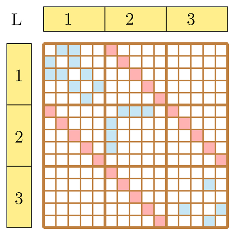
Temporal networks have a special property of having the inter-layer coupling only between adjacent layers. Which means that the network can have inter-layer edges only between layers {α, α ± 1}. This special kind of coupling leads to diagonal blocks in non-diagonal positions (adjacent to diagonal blocks) of the supra-adjacency matrix as shown in Fig. 3. To extend the existing centrality measures to temporal networks, one obvious way is to use the NL × NL supra-adjacency matrix with different attention to the interlayer edges,

$$A=\left[\begin{array}{c}{A}^{[1]}\omega (I)0\cdots \\ \omega (I)A^{[2]}\omega (I)\ddots \\ 0\omega (I)A^{[3]}\ddots \\ ⋮\ddots \ddots \ddots \end{array}\right]$$

Figure 3. Supra-adjacency matrix representation of multilayer network shown in Fig. 4 .

where ω ≥ 0 is known as the layer coupling coefficient. Traditional centrality measures can directly be applied on A which will lead to a centrality vector of size NL. The centrality vector can be interpreted to return the node centrality at each time stamp⁵. Clearly, this approach ignores the block diagonal structure of the matrix and does not distinguish between the inter-layer and intra-layer edges¹⁰. This issue can be circumvented by changing the representation of either the inter-layer edges or the intra-layer edges. We discuss both of these methods below:

3.1.1. Inter-Layer Coupling of Centrality Matrices

The idea of this approach is to find the centrality matrix for each layer and directly couple it to the centrality matrix of its adjacent temporal layers. Let C ^[α] denote the centrality matrix for the temporal network at layer α. Let ϵ = 1/ω Then the supra-centrality matrix⁴⁸ can be represented as,

$$ℂ=\left[\begin{array}{cccc}{C}^{[1]}& I& 0& \cdots \\ I& C^{[2]}& I& \ddots \\ 0& I& C^{[3]}& \ddots \\ ⋮& \ddots & \ddots & \ddots \end{array}\right]$$

The above formulation works with the assumption that C^[α] is non-negative and irreducible for every α ∈ L. Similarly, C is also non-negative and irreducible for any ε > 0, which leads to the Perron Frobenius theorem for non-negative matrices³¹ and ensures uniqueness of the largest eigenvalue and non-negativity of the corresponding eigenvector⁵². Thus, the C matrix can be viewed as an adjacency matrix to find centrality using standard methods.

3.1.2. Incorporating Inter-Layer Similarity

Let $C^{[\alpha ,\alpha +1]}=diag\left(c_1^{[\alpha ,\alpha +1]},c_2^{[\alpha ,\alpha +1]},\dots ,c_N^{[\alpha ,\alpha +1]}\right)$ be the N × N dimensional inter-layer similarity matrix for layers α and α + 1. The supra-adjacency matrix can then be formulated⁵² as:

$$A=\left[\begin{array}{cccc}{A}^{[1]}& C^{[1,2]}& 0& \dots \\ C^{[2,1]}& A^{[2]}& C^{[2,3]}& \ddots \\ 0& C^{[2,3]}& A^{[3]}& \ddots \\ ⋮& \ddots & \ddots & \ddots \end{array}\right]$$

where $c_i^{\alpha ,\alpha +1}$ denotes the similarity between the same physical node at two adjacent layers. The supra-adjacency matrix A can now be used to find the centrality. There are many similarity measures to compute $c_i^{\alpha ,\alpha +1}$ such as Adamic-Adar Index¹, Jaccard Index, Salton Index²⁰, Resource Allocation Index⁵⁶, etc. For a detailed experimental study on this method, kindly refer to⁵².

3.2. Diagonal Coupling

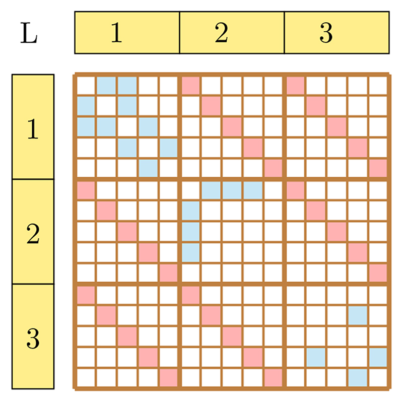
In time-independent multilayer networks, the inter-layer coupling is not limited to adjacent layers. For example, a multilayer network can represent different relationships among authors such as citation, co-authorship, co-citation, etc. In such networks, one can observe inter-layer coupling among all pairs of layers as shown in Fig. 5. Without loss of generality, one can assume the same set of vertices but a possibly different set of edges in different layers. Finding centrality in such networks has multiple applications such as node ranking⁴², finding the most versatile nodes¹¹, etc. For the same reason, multilayer centrality is also referred to as versatility. In the current section, we discuss two major approaches to find centrality— eigenvector-based and path-based.

Figure 5. Supra-adjacency matrix representation of multilayer network as shown in Fig. 6.

3.2.1. Eigenvector-Based Centrality

Network structure in layer α may get influenced by the nodes from other layers α^′. The centrality measure for multilayer network must take this influence into account. This influence among layers can be captured by a matrix W ∈ ℝ^L×L, where w_αβ denotes the influence of layer α on layer β. Once the w_αβ is fixed, we can define the local multilayer eigenvector-like centrality c_α as a leading eigenvector of the following matrix:

$$A_{\alpha }=\beta w_{\alpha \beta }{A}^{[\beta ,\beta ]}$$

Now, we can directly use this matrix to find centrality with traditional methods.

Sometimes, centrality of a node v in a layer not only depends on the other connected nodes in the same layer α but also on the nodes from other layers. In such networks, it becomes essential to consider the influence from the nodes across the layers. To find the centrality of a node in a particular layer, the following modified adjacency matrix can be used⁴³.

$$\begin{array}{c}{A}^{\otimes }=\left[\begin{array}{cccc}{w}_{11}{A}^{[1,1]}& w_{12}{A}^{[2,2]}& \dots & w_{1L}{A}^{[L,L]}\\ w_{21}{A}^{[1,1]}& w_{22}{A}^{[2,2]}& \dots & w_{2L}{A}^{[L,L]}\\ ⋮& ⋮& \ddots & ⋮\\ w_{L1}{A}^{[1,1]}& w_{L2}{A}^{[2,2]}& \dots & w_{LL}{A}^{[L,L]}\end{array}\right]\\ \in {ℝ}^{NL\times NL}\end{array}$$

Where A^⊗ is the Khatri-Rao product of the following matrices:

$$W=\left[\begin{array}{ccc}{w}_{11}& \dots & w_{1L}\\ ⋮& \ddots & ⋮\\ w_{L1}& \dots & w_{LL}\end{array}\right]\text{and}\left(A^{[1,1]}{A}^{[2,2]}\dots A^{[L,L]}\right)$$

A^⊗ can be viewed as a giant adjacency matrix and can be used to find centrality by the measures defined on monoplex networks. To read up on the existence and uniqueness of the leading eigenvector of A^⊗, please refer to⁴³.

3.2.2. Path-Based Centrality

Betweenness centrality is a prominent path-based centrality measure. To extend betweenness

centrality measure to multilayer networks, we have to accommodate the fact that a path can comprise of nodes and edges from multiple layers. Let σ_iα_jβ be the count of edge distinct shortest paths from (i, α) to (j, β). The cross betweenness centrality C(v) of a node-layer pair (v, μ) is defined as the fraction of times (v, μ) occurs on the shortest path between any origin–destination pair {(i, α), (j, β)}. Mathematically,

$$C\left(v^{\mu }\right)=i,j\in V:i\ne j\left(\alpha \in L\frac{{\sigma }_{i^{\alpha }{j}^{\alpha }}^{\nu }}{{\sigma }_{i^{\alpha }{j}^{\alpha }}}+(1-)\alpha ,\beta \in L:\alpha \ne \beta \frac{{\sigma }_{i^{\alpha }{j}^{\beta }}^{{\nu }^{\mu }}}{{\sigma }_{i^{\alpha }{j}^{\beta }}}\right)$$

where ${\sigma }_{i^{\alpha }{j}^{\beta }}^{v^{\mu }}$ is the number of times node–layer pair (v, μ) occurs on the shortest path from (i, α) to (j, β). Here ε is a tuning parameter which balances between the importance of inter-layer and intra-layer edges. Cross betweenness centrality of a node can be computed in O(NLE) ⁷.

3.3. Cross Coupling

This is the most general case of coupling among all the methods discussed in this article. A node– layer pair (i, α) can be influenced by the nodes in the same layer ((j, α) : i = j) as well as nodes of any other layer ((j, β) : α = β) as shown in Fig. 1. Note that the coupling techniques discussed in earlier sections are the special cases of this particular coupling, which makes it important to extend (or reformulate) the centrality measures for these networks. We do so by adopting as is the framework of random walk on weighted (monoplex) graphs, and only changing the graph on which this framework is applied (viz., applying this random walk framework as is to a large weighted graph constructed out of our multilayer network as described below).

To define the centrality measures first, we introduce the random walk operator for a multilayer network M = (V_M, E_M, V, L). A weighted multilayer network can have weights associated to the edges. Let wij(α, β) be the weight of the edge between (i, α) and (j, β). Let $s_{i\alpha }=j,\beta w_{ij}(\alpha ,\beta )$ be the node strength of (i, α). We can write the transition probability from (i, α) to (j, β) as

$$T_{j\beta }^{i\alpha }=\frac{w_{ij}(\alpha ,\beta )}{\max \left(s_{i\alpha },\right)}$$

where ϵ > 0 is a constant. Note that is a fourdimensional matrix (also known as tensor). At time t, let piα (t) be the probability of finding the random walker at (i, α).Then,

$$p_{j\beta }(t+1)=(i,\alpha )\in V_M{T}_{j\beta }^{i\alpha }{p}_{i\alpha }(t)$$

The steady state solution for the random walk can be given by the leading eigentensor ⁴⁴,

$$T_{j\beta }^{i\alpha }{\text{Π}}_{i\alpha }=\lambda {\text{Π}}_{j\beta }$$

Intuitively a random walker should visit the nodes with high strength more frequently than the nodes with lesser strength. This is also evident from our formulation as, ${\pi }_{i\alpha }\propto s_{i\alpha }$. The transition tensor $T_{j\beta }^{i\alpha }$ can be defined in multiple ways⁹, but in this article we focus on the one similar to a random walk on monoplex networks³⁵.

We can use this formulation to define different centrality measures on multilayer networks. Following the discussion from¹¹, in PageRank, a walker can move from one node to its neighbor with probability r and it can teleport to any other node with probability (1 - r). Considering the uniform probability of getting a node picked while teleportation, the transition tensor can be given by,

$$R_{j\beta }^{i\alpha }=r{T}_{j\beta }^{i\alpha }+\frac{(1-r)}{NL}{u}_{j\beta }^{i\alpha }$$

where $u_{j\beta }^{i\alpha }$ is the unit tensor of rank 4. PageRank centrality for multilayer networks is given by the solution of this master equation. As we discussed in Sect. 3.2.2, betweenness centrality is another important centrality measure. There we measured the betweenness centrality as the fraction of times a node j occurs on all pair shortest paths. However, in many real-world networks, information does not necessarily propagate through the shortest path. For example, packets over the internet or rumors over a social network are not always restricted to following the shortest path^{15, 47}. In such cases, the shortest path betweenness centrality is not the right choice to make. One possible proxy for the betweenness is the random-walk betweenness, which is the number of random walks between any pair of nodes that pass through a node j ³³. To analytically compute this number, it is convenient to use the absorbing random walk. Since we are interested in counting the number of times a node j appears on the random walk, we assume node v as the absorbing state. For multilayer networks, we can define an absorbing random walk by the following 4-rank tensor,

$${\left(T_{[v]}\right)}_{j\beta }^{i\alpha }=\{\begin{array}{c}0\text{if}j=v\\ T_{j\beta }^{i\alpha }\text{otherwise}\end{array}$$

Following the discussion from⁴⁴, the number of times a random walker passes through a node j in layer β, irrespective of time step, is given by,

$${\left({\tau }_{[v]}\right)}_{j\beta }^{i\alpha }={\left[{\left(\delta -T_{[d]}\right)}^{-1}\right]}_{j\beta }^{i\alpha }$$

where δ is a 4 - d tensor such that ${\delta }_{j\beta }^{i\alpha }={\delta }_j^i{\delta }_{\beta }^{\alpha }$ and δ represents the Kronecker delta. It can be noticed that the number of times the random walker visits node j depends on the layers where j and starting node are located. Let o be the starting node, the matrix representation of a random walker which can start from any layer σ and pass through j in any layer is given by,

$${\left({\tau }_{[v]}\right)}_j^o=\frac{1}{L}{\left({\tau }_{[v]}\right)}_{j\beta }^{o\sigma }{u}^{\beta }{u}_{\sigma },$$

where u^β and uσ are unit column vector and unit row vector, respectively. The final betweenness centrality vector can be obtained by averaging over all possible origin–destination pairs as follows,

$${\tau }_j=\frac{1}{N(N-1)}Nv=1{\left({\tau }_{[v]}\right)}_j^o{u}_o$$

For theoretical justification and empirical evidences kindly refer to⁴⁴. In addition to using the supra-adjacency list and supra-adjacency matrix representation of multilayer networks, there are other popular approaches such as representing the multilayer network as a collection of nodes and multilinks²³. To observe the effect of inter-layer cross-coupling on a node, one can find the centrality using the measures defined in this section and subtract it from the centrality calculated by the measures defined in the previous sections.

4. Conclusion

Multilayer networks can capture multiple types of interactions among nodes. Due to the variety of applications of multilayer networks, different aspects of these networks have been studied such as their robustness against node attacks^{13, 54, 55}, process spreading^{8, 50} and evolutionary games⁵¹. In this paper, we discussed different types of inter-layer coupling in multilayer networks, their use-cases, and their implications on centrality measures. Currently, the study of multilayer networks is confined to layers which capture homogeneous entities and their pairwise relationships to one another. Many complex systems are better modelled by other richer graph structures such as hypergraphs^{28, 38, 40}, and knowledge graphs^{34, 37}. It can be a promising future direction to extend the multilayer network framework to capture such complex graph structures and study their properties.

Figure 4. A multilayer network depicting the diagonal inter-layer coupling of adjacent layers, for example, time-series points.

Figure 6. A multilayer network depicting the diagonal inter-layer coupling. Every node in a layer is connected to its counterpart in all other layers.

Biographies

Tarun Kumar is a Ph.D. Scholar at the Department of Computer Science and Engineering, Indian Institute of Technology Madras where he is jointly co-advised by Prof. Balaraman Ravindran and Prof. Manikandan Narayanan. His research interests lie at the intersection of Machine Learning and Network Science. Specifically, he is intrigued by the dynamics of systems comprising higher order interactions. He received his M.Tech. from the Department of Computer Science and Engineering, School of Engineering Sciences, Shiv Nadar University (First Rank). Tarun enjoys giving interdisciplinary talks; for instance, he gave a presentation in the 4th IBSE workshop at IIT Madras where the audience was prominently from the Biology background and he won the best presentation award.

Manikandan Narayanan enjoys research at the interface between computer science and systems biology in his current position as an associate professor at the Indian Institute of Technology Madras. He is fascinated with using the power of computation and network/data-driven science to tease apart the molecular interactions underlying life, and his research focuses specifically on (multilayer) graph algorithms and probabilistic models to discover novel tissue–tissue communication or disease–disease interaction routes from high-dimensional genomic data. He obtained his Ph.D. in Computer Science (with an emphasis in computational and genomic biology) from the University of California at Berkeley and held a Sr. Research Scientist position at Merck Research Labs before joining National Institutes of Health (NIH) as a Staff Scientist. He is a Siebel Scholar Class of 2003, author of well-cited publications in computational/systems biology journals, and a WellcomeTrust/DBT India Alliance Intermediate Fellow starting 2017. His current research interests and contributions all started with his exposure to research as a summer JNCASR intern at the Indian Institute of Science (IISc) at Bangalore and his undergraduate computer science training at College of Engineering, Anna University, Guindy.

Balaraman Ravindran is a professor at the Department of Computer Science and Engineering and heads the Robert Bosch Centre for Data Science and AI at the Indian Institute of Technology Madras. He completed his Ph.D. at the Department of Computer Science, University of Massachusetts, Amherst. He worked with Prof. Andrew G. Barto on an algebraic framework for abstraction in reinforcement learning. His current research interests span the broader area of machine learning, ranging from spatio-temporal abstractions in reinforcement learning to social network analysis and data/text mining. Much of the work in his group is directed toward understanding interactions and learning from them.

References

- 1.Adamic LA, Adar E. Friends and neighbors on the web. Social networks. 2003;25(3):211–230. [Google Scholar]
- 2.Aleta A, Meloni S, Moreno Y. A multilayer perspective for the analysis of urban transportation systems. Sci Rep. 2017;7:44359. doi: 10.1038/srep44359. [DOI] [PMC free article] [PubMed] [Google Scholar]
- 3.Aleta A, Moreno Y. Multilayer networks in a nutshell. arXiv preprint arXiv. 2018:1804.03488 [Google Scholar]
- 4.Battiston F, Nicosia V, Latora V. The new challenges of multiplex networks: measures and models. Euro Phys J Spec Top. 2017;226(3):401–416. [Google Scholar]
- 5.Bazzi M, Porter MA, Williams S, McDonald M, Fenn DJ, Howison SD. Community detection in temporal multilayer networks, with an application to correlation networks. Multiscale Model Simul. 2016;14(1):1–41. [Google Scholar]
- 6.Boccaletti S, Bianconi G, Criado R, Del Genio CI, Gómez-Gardenes J, Romance M, Sendina-Nadal I, Wang Z, Zanin M. The structure and dynamics of multilayer networks. Phys Rep. 2014;544(1):1–122. doi: 10.1016/j.physrep.2014.07.001. [DOI] [PMC free article] [PubMed] [Google Scholar]
- 7.Chakraborty T, Narayanam R. Cross-layer betweenness centrality in multiplex networks with applications; Data engineering (ICDE), 2016 IEEE 32nd international conference on; 2016. pp. 397–408. [Google Scholar]
- 8.De Domenico M, Granell C, Porter MA, Arenas A. The physics of spreading processes in multilayer networks. Nat Phys. 2016;12(10):901. [Google Scholar]
- 9.De Domenico M, Solé A, Gómez S, Arenas A. Random walks on multiplex networks. arXiv preprint arXiv. 2013:1306.0519 [Google Scholar]
- 10.De Domenico M, Solé-Ribalta A, Cozzo E, Kivelä M, Moreno Y, Porter MA, Gómez S, Arenas A. Mathematical formulation of multilayer networks. Phys Rev X. 2013;3(4):041022 [Google Scholar]
- 11.De Domenico M, Solé-Ribalta A, Omodei E, Gómez S, Arenas A. Ranking in interconnected multilayer networks reveals versatile nodes. Nat Commun. 2015;6:6868. doi: 10.1038/ncomms7868. [DOI] [PubMed] [Google Scholar]
- 12.De Meo P, Ferrara E, Fiumara G, Ricciardello A. A novel measure of edge centrality in social networks. Knowl Based Syst. 2012;30:136–150. [Google Scholar]
- 13.Demeester P, Gryseels M, Autenrieth A, Brianza C, Cast-agna L, Signorelli G, Clemenfe R, Ravera M, Jajszczyk A, Janukowicz D, et al. Resilience in multilayer networks. IEEE Commun Mag. 1999;37(8):70–76. [Google Scholar]
- 14.Dolev S, Elovici Y, Puzis R. Routing betweenness centrality. J ACM (JACM) 2010;57(4):25. [Google Scholar]
- 15.Freeman LC, Borgatti SP, White DR. Centrality in valued graphs: A measure of betweenness based on network flow. Soc Netw. 1991;13(2):141–154. [Google Scholar]
- 16.Gallotti R, Barthelemy M. The multilayer temporal network of public transport in great britain. Sci Data. 2015;2:140056. doi: 10.1038/sdata.2014.56. [DOI] [PMC free article] [PubMed] [Google Scholar]
- 17.Gleich DF. Pagerank beyond the web. SIAM Rev. 2015;57(3):321–363. [Google Scholar]
- 18.Gomez S, Diaz-Guilera A, Gomez-Gardenes J, Perez-Vicente CJ, Moreno Y, Arenas A. Diffusion dynamics on multiplex networks. Phys Rev Lett. 2013;110(2):028701. doi: 10.1103/PhysRevLett.110.028701. [DOI] [PubMed] [Google Scholar]
- 19.Halu A, De Domenico M, Arenas A, Sharma A. The multiplex network of human diseases. bioRxiv. 2017:100370. doi: 10.1038/s41540-019-0092-5. [DOI] [PMC free article] [PubMed] [Google Scholar]
- 20.Hamers L, et al. Similarity measures in scientomet-ric research: The jaccard index versus salton’s cosine formula. Inf Process Manag. 1989;25(3):315–18. [Google Scholar]
- 21.Hilary. Centrality measures in multilayer networks. University of Oxford; 2015. https://people.mathsox.acuk/porterm/research/Flora_BEE_Submitted-032315.pdf. [Google Scholar]
- 22.Hristova D, Williams MJ, Musolesi M, Panzarasa, Mas-colo C. Measuring urban social diversity using interconnected geo-social networks; Proceedings of the 25th international conference on world wide web; 2016. pp. 2–30. [Google Scholar]
- 23.Iacovacci J, Rahmede C, Arenas A, Bianconi G. Functional multiplex pagerank. EPL (Euro Lett) 2016;116(2):28004. [Google Scholar]
- 24.Joseph A, Chen G. Composite centrality: a natural scale for complex evolving networks. Physica D. 2014;267:58–67. [Google Scholar]
- 25.Kanawati R. Multiplex network mining: a brief survey. IEEE Intell Inform Bull. 2015;16(1):24–27. [Google Scholar]
- 26.Kim H, Anderson R. Temporal node centrality in complex networks. Phys Rev E. 2012;85(2):026107. doi: 10.1103/PhysRevE.85.026107. [DOI] [PubMed] [Google Scholar]
- 27.Kivelä M, Arenas A, Barthelemy M, Gleeson JP, Moreno Y, Porter MA. Multilayer networks. J Complex Netw. 2014;2(3):203–271. [Google Scholar]
- 28.Klamt S, Haus UU, Theis F. Hypergraphs and cellular networks. PLoS Comput Biol. 2009;5(5):e1000385. doi: 10.1371/journal.pcbi.1000385. [DOI] [PMC free article] [PubMed] [Google Scholar]
- 29.Liao H, Mariani MS, Medo M, Zhang YC, Zhou MY. Ranking in evolving complex networks. Phys Rep. 2017;689:1–54. [Google Scholar]
- 30.Liu S, Chen PY, Hero A, Rajapakse I. Dynamic network analysis of the 4d nucleome. bioRxiv. 2018:268318 [Google Scholar]
- 31.Meyer CD. Matrix analysis and applied linear algebra. Society for Industrial and Applied Mathematics; Philadelphia, PA, USA: 2000. [Google Scholar]
- 32.Newman M. Networks. 2nd. Oxford University Press, Inc; New York, NY, USA: 2018. [Google Scholar]
- 33.Newman ME. A measure of betweenness centrality based on random walks. Soc Netw. 2005;27(1):39–54. [Google Scholar]
- 34.Nickel M, Murphy K, Tresp V, Gabrilovich E. A review of relational machine learning for knowledge graphs. Proc IEEE. 2016;104(1):11–33. [Google Scholar]
- 35.Noh JD, Rieger H. Random walks on complex networks. Phys Rev Lett. 2004;92(11):118701. doi: 10.1103/PhysRevLett.92.118701. [DOI] [PubMed] [Google Scholar]
- 36.Pilosof S, Porter MA, Pascual M, Kéfi S. The multilayer nature of ecological networks. Nat Ecol Evolut. 2017;1(4):0101. doi: 10.1038/s41559-017-0101. [DOI] [PubMed] [Google Scholar]
- 37.Popping R. Knowledge graphs and network text analysis. Soc Sci Inform. 2003;42(1):91–106. [Google Scholar]
- 38.Ramadan E, Tarafdar A, Pothen A. A hypergraph model for the yeast protein complex network; Parallel and distributed processing symposium, 2004. Proceedings 18th international; 2004. p. 189. [Google Scholar]
- 39.Rysz M, Pajouh FM, Pasiliao EL. Finding clique clusters with the highest betweenness centrality. Euro J Oper Res. 2018;271(1):155–164. doi: 10.1016/Jejor2018.05.006. [DOI] [Google Scholar]
- 40.Satchidanand SN, Ananthapadmanaban H, Ravindran B. In: Yang Y, Wooldridge M, editors. Extended discriminative random walk: a hypergraph approach to multi-view multi-relational transduc-tive learning; Proceedings of the 24th international conference on artificial intelligence, IJCAI’15; Buenos Aires, Argentina. 2015. pp. 3791–3797. [Google Scholar]
- 41.Shinde, Jalan S. A multilayer protein-protein interaction network analysis of different life stages in cae-norhabditis elegans. EPL (Europhys Lett) 2015;112(5):58001. [Google Scholar]
- 42.Sideris G, Katsaros D, Sidiropoulos A, Manolopoulos Y. The science of science and a multilayer network approach to scientists’ ranking; Proceedings of the 22nd international database engineering &; applications symposium; 2018. pp. 5–11. [Google Scholar]
- 43.Solá L, Romance M, Criado R, Flores J, Garcíadel Amo A, Boccaletti S. Eigenvector centrality of nodes in multiplex networks Chaos: an Interdisciplinary. J Nonlinear Sci. 2013;23(3):033131. doi: 10.1063/1.4818544. [DOI] [PubMed] [Google Scholar]
- 44.Solé-Ribalta A, De Domenico M, Gómez S, Arenas A. Random walk centrality in interconnected multilayer networks. Physica D. 2016;323:73–79. [Google Scholar]
- 45.Solé-Ribalta A, Gómez S, Arenas A. Congestion induced by the structure of multiplex networks. Phys Rev Lett. 2016;116(10):108701. doi: 10.1103/PhysRevLett.116.108701. [DOI] [PubMed] [Google Scholar]
- 46.Sorz J, Wallner B, Seidler H, Fieder M. Inconsistent year-to-year fluctuations limit the conclusiveness of global higher education rankings for university management. Peer J. 2015;3:e1217. doi: 10.7717/peerj.1217. [DOI] [PMC free article] [PubMed] [Google Scholar]
- 47.Stephenson K, Zelen M. Rethinking centrality: methods and examples. Soc Netw. 1989;11(1):1–37. [Google Scholar]
- 48.Taylor D, Myers SA, Clauset A, Porter MA, Mucha PJ. Eigenvector-based centrality measures for temporal networks. Multiscale Model Simul. 2017;15(1):537–574. doi: 10.1137/16M1066142. [DOI] [PMC free article] [PubMed] [Google Scholar]
- 49.Türker Ì, Sulak EE. A multilayer network analysis of hashtags in twitter via co-occurrence and semantic links. Int J Mod Phys B. 2018;32(04):1850029 [Google Scholar]
- 50.Wang W, Liu QH, Cai SM, Tang M, Braunstein LA, Stanley HE. Suppressing disease spreading by using information diffusion on multiplex networks. Sci Rep. 2016;6:29259. doi: 10.1038/srep29259. [DOI] [PMC free article] [PubMed] [Google Scholar]
- 51.Wang Z, Wang L, Szolnoki A, Perc M. Evolutionary games on multilayer networks: a colloquium. Euro Phys J B. 2015;88(5):124. [Google Scholar]
- 52.Yin R-R, Guo Q, Yang J-N, Liu J-G. Inter-layer similarity-based eigenvector centrality measures for temporal networks. Physica A Stat Mech Appl. 2018;512:165–173. doi: 10.1016/Jphysa.2018.08.018. [DOI] [Google Scholar]
- 53.Zhang H, Zhang H, Thai MT. Big data in complex and social networks. Chapman and Hall/CRC; 2016. A survey on multilayer networks and the applications; pp. 193–222. [Google Scholar]
- 54.Zhao D, Wang Z, Xiao G, Gao B, Wang L. The robustness of interdependent networks under the interplay between cascading failures and virus propagation. EPL (Europhys Lett) 2016;115(5):58004. [Google Scholar]
- 55.Zhao DW, Wang LH, Zhi YF, Zhang J, Wang Z. The robustness of multiplex networks under layer node-based attack. Sci Rep. 2016;6:24304. doi: 10.1038/srep24304. [DOI] [PMC free article] [PubMed] [Google Scholar]
- 56.Zhou T, Lü L, Zhang YC. Predicting missing links via local information. Euro Phys J B. 2009;71(4):623–630. [Google Scholar]