Abstract
Knowing the extent and environmental drivers of forests is key to successfully restore degraded ecosystems, and to mitigate climate change and desertification impacts using tree planting. Water availability is the main limiting factor for the development of forests in drylands, yet the importance of groundwater resources and paleoclimate as drivers of their current distribution has been neglected. Here we report that mid-Holocene climates and aquifer trends are key predictors of the distribution of dryland forests worldwide. We also updated the global extent of dryland forests to 1283 million hectares and showed that failing to consider past climates and aquifers has resulted in ignoring or misplacing up to 130 million hectares of forests in drylands. Our findings highlight the importance of a wetter past and well-preserved aquifers to explain the current distribution of dryland forests and can guide restoration actions by avoiding unsuitable areas for tree establishment in a drier world.
Dryland forests are essential for the survival of the poorest human populations on our planet, which strongly rely on woody vegetation for obtaining fuel, shelter and food1. Reductions in soil water availability2 associated with forecasted increases in aridity3 and in the number and duration of droughts4 are expected to reduce the area of drylands capable of supporting forest ecosystems5. Despite so, many dryland regions, especially in China6 and Africa7, are important candidates for global ecosystem restoration initiatives associated with the UN Decade of Ecosystem Restoration 2021-20308. Trees in drylands typically use more water than grasses or shrubs9, so afforestation may reduce water availability for essential human activities such as agriculture10, resulting in water shortages that could lead to local and regional conflicts11,12. Because of this, identifying those drylands capable of supporting forests is essential to guide current and future restoration efforts, so they can maximize the multiple benefits of forests while minimizing the risk of water scarcity in these areas.
Despite important recent advances to understand the distribution of dryland forests13, their definitive extent is far from being fully understood. For example, a recent study14 found an unexpected number of trees in the Sahel, where numerous efforts involving the restoration of complex ecosystems are underway under the umbrella of the Africa’s Great Green Wall15. We posit that current discrepancies in forest extent are based on the lack of consideration of key factors influencing the development of trees in drylands. In contrast to forests located in humid areas, the distribution dryland forests is highly constrained by their typically low water availability and high evapotranspiration rates16. However, not all current drylands have experienced the same dry climate over millennia, and many of them come from a wetter past17. Paleoclimatic conditions are known to influence the current structure and functioning of terrestrial ecosystems18,19 and may have influenced the establishment of dryland forests over millennia20. Locations with wetter past conditions might thus have allowed the establishment of dryland forests, which otherwise might not exist under today’s drier climates. However, empirical evidence supporting this is lacking. Similarly, the presence of local shallow aquifers –many of those located in drylands are a relic from a wetter past– influences 22-32% of the global land surface21, and has been found to influence the distribution of forests in particular drylands22. Remarkably, the role of past climates and groundwater resources as predictors of the current distribution of dryland forests at the global scale is poorly understood and has not been evaluated yet.
Here we combine a unique very high-resolution (<1 m/pixel) imagery dataset of 94,352 dryland plots (0.5 ha), with information on climate23, aquifer trends24, soil properties25, environmental factors, land use maps26,27, and vegetation height28 to: i) quantify the relative importance of current and past (mid-Holocene; 6000 years before present) climate, aquifers and other key environmental predictors (Supplementary Table 1) associated with the current distribution of forests across global drylands; ii) provide an accurate and updated distribution of dryland forests worldwide; iii) compare the current extent of dryland forests with the maps of tree restoration potential29; and iv) forecast the future (2081-2100) extent of dryland forests according to multiple socio-economic and climate change scenarios. These are fundamental steps to advance our knowledge about the extent and predictors of forest ecosystems across global drylands, which cover ~41% of the Earth's land surface30, to maximize the socio-economic and ecological benefits of afforestation efforts, and to inform policies to mitigate climate change and desertification.
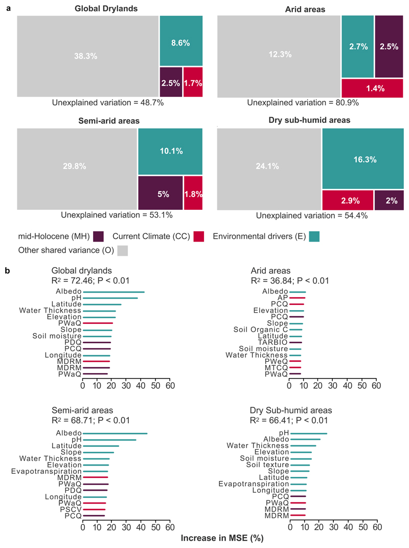
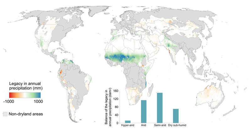
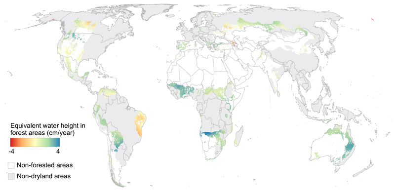
In general, mid-Holocene precipitation and temperature (Fig. 1) and climatic legacies (differences in precipitation and temperature between past and current climates) predicted a unique and significant proportion of the variation in the distribution of current forests in drylands (variation partitioning analyses, see Methods, Fig. 1a). These findings were particularly evident in semi-arid regions, which had a wetter climate in the mid-Holocene than today31 (Extended Data Fig. 1). Similar results were found when using an alternative machine learning approach (Random Forest modelling, see Methods) to quantify the importance of the variables studied (Fig. 1b). Our analyses show that locations with higher increases in precipitation since the mid-Holocene, particularly in the warmest, driest, and coldest quarters, hold more forests now than should be expected according to their current climatic conditions. Moreover, areas that have suffered from larger increases in temperature over the last 6000 years support fewer forests today. Our results thus provide new evidence on the importance of past climates as a major predictor of the current distribution of dryland forests worldwide. The presence and evolution of aquifers (measured by water thickness over the period 2002-2017, see Methods) was also a key factor explaining the current distribution of dryland forests (Fig. 1b). Almost half of the forests in drylands, 613 million hectares (Mha), are growing over aquifers where the piezometric level has declined21 (Extended Data Fig. 2). These include forests found mainly in zones of eastern Brazil, central Canada, northern Mexico, southeastern Russia, and the southwestern United States of America. These areas thus may not be able to support forests in the future, given the enhanced aridity and the increased duration and intensity of drought periods expected for many of them5.
Fig. 1. Relative contribution of past climate (mid-Holocene, 6000 years before present), current climate, and other environmental variables as drivers of the current distribution of dryland forests worldwide.
a, Results from variation partitioning modelling aiming to identify the percentage of the variance of forest distribution explained by each predictor. b, Results from random forest analysis aiming to identify the top fourteen significant (P < 0.01; for one-sided testing) variables regulating forest distribution across global drylands. An increase in the percentage of Mean Squared Error in variables equals more importance. Acronyms are available in Supplementary Table 1.
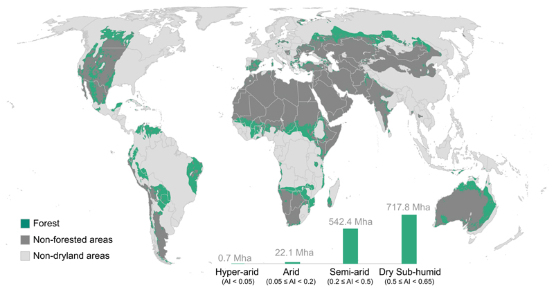
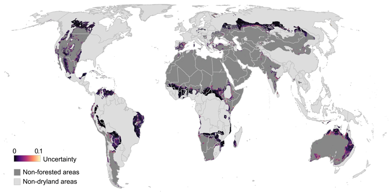
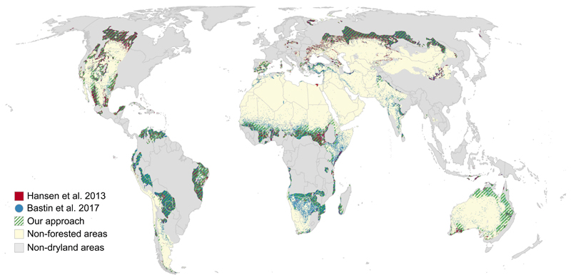
We found that drylands are covered by 1283 (±15) Mha of forests, excluding tree plantations (Fig. 2). Forests occupy 717.8, 542.4, 22.1 and 0.7 Mha of dry sub-humid, semi-arid, arid, and hyper-arid areas, respectively, and represent ~19% of the surface of global drylands. The confidence of these estimates was highest in areas with a high probability of finding forest (i.e., the models agreed on areas of bare soil or very dense forests, such as the Sahara Desert or the forests in South America). In contrast, areas with low confidence were those with low or medium probability (less than 50%, the threshold used to classify forest/non-forest; Extended Data Fig. 3). Compared with the most recent estimates available13,32, our estimates increase the global forest area in drylands by ~200 Mha. Even more importantly, our forest map changed the location of ~33% of dryland forest area compared to the most recent global estimates13,32, suggesting that ⅓ of forests were misplaced by them (Extended Data Fig. 4). The main reasons for these differences are likely related to the modelling approach we used, which combines the explicit consideration of past climate and groundwater trends with high-resolution imagery and discarded areas covered by large shrubs (see Methods).
Fig. 2. The distribution of forests across global drylands considering climate legacies (changes in climate over the last 6000 years) and aquifer trends.
Forest areas are those with a probability > 50% according to the Random Forest approach used (see Methods). AI = aridity index.
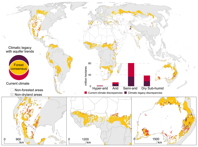
To further illustrate the importance of past climates and aquifers as drivers of the current distribution of forests in drylands, we located the extent of forest in drylands considering or not past climate and aquifer trends. The consensus between the forest maps considering or excluding climatic legacies and aquifer trends was 1225 Mha (Fig. 3). The discrepancies in these maps added up to ~130 Mha, equivalent to 3.7 billion trees14 or the equivalent of the total area of France, Italy, the United Kingdom, Switzerland, Netherlands, and Belgium together. These discrepancies were mainly located in areas where paleoclimatic legacies were especially important, which include the Sahel, south Australia, Mexico, and the Southwest of the United States of America (Fig. 3). The presence of many of these forests cannot simply be explained without considering paleoclimates and aquifer trends. The importance of past climates as drivers of the distribution of current forests was more noticeable in semi-arid regions across the globe (Fig. 3), with over 81 Mha of forests being neglected or misplaced by models based only on current climatic conditions. Over 31 Mha of these forests are moreover located in the transition between arid and semiarid regions (Aridity Index = 0.2), which has recently been reported to be a threshold driving abrupt changes33 in multiple ecosystems attributes, including a decline in vegetation cover and richness, across global drylands34. Planting trees in these transitional regions should be done with extreme caution and even avoided where it could accelerate the depletion of groundwater resources and jeopardize water availability for other organisms and human uses, as is already occurring in areas where extensive afforestation programs have been established over the last decades, such as the Chinese Loess Plateau10.
Fig. 3. Comparison between the extent of forests calculated with and without considering the effects of climatic legacies and aquifer trends.
Consensus areas are shown in yellow. Discrepancies in forest extent when considering climatic legacies (changes in climate over the last 6000 years) and aquifer trends are shown in purple. Discrepancies in forest extent when considering current climate only are shown in red.
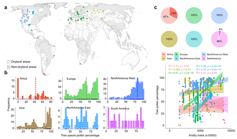
The existence of dryland forests may be explained by different causes. They can be relict forests in which recruiting is being hampered by current conditions but their survival is not. If so, the trees in these areas would be old and simply a very long transient state towards conversion into a non-forested vegetation35. However, since the trees in these areas would be at least 6000 years old and these ages are uncommon for many tree species, this cause can probably be overruled. A more plausible explanation is that forests in these areas are stable configurations that can survive and recruit under current conditions, even if they do so at the edge of their optimal environmental suitability. To check whether trees existed in the locations where forests exist today in the mid-Holocene, we explored data from LegacyPollen v.136, a harmonization of paleo-pollen databases. We found pollen samples (n=1121) of tree species aged 5000-7000 years at 119 sites located in current dryland forests from six large regions (Africa, Asia, East of North America, Europe, South America, and West of North America; Extended Data Fig. 5a). The median of the percentage of pollen from tree species was more than 40% in these regions (Extended Data Fig. 5b), and samples with more than 5% tree species pollen were found in 93% of the cases (Asia 100%, Europe 100%, North America 100%, Africa 67%, and South America 96%). We observed a significant negative relationship between the % of tree species present in the pollen samples and aridity across Europe, East of North America, and West of North America (Extended Data Fig. 5c). These findings suggest that most dryland areas sustaining forests today already had a prevalence of forest vegetation in the mid-Holocene and that the dominance of tree species decreased as aridity increased back then (as it happens today). Although these findings cannot provide a definitive proof, they suggest the presence of hysteretic behaviour in dryland forests (i.e., forests inherited from the past do not revert to non-forest states even when environmental conditions suggest that this would be the most reasonable). This type of hysteretic behaviour has already been found in tropical forests37. If true for dryland forests, this would suggest the existence of some type of forest-specific stabilizing mechanism that allows forests to thrive in drylands. Potential stabilizing mechanisms include hydroclimatic feedbacks37 and the modification of the surrounding physical environment by trees38, which create suitable conditions for tree development.
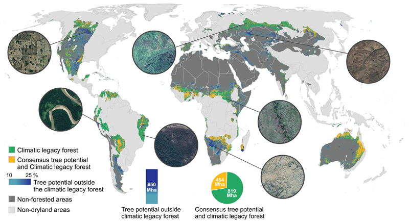
By identifying climatic legacies and aquifers as important factors explaining the current distribution of forests across global drylands, our findings have important implications for their restoration. The comparison of the current forest extent in drylands, as revealed by our results, with tree restoration potential maps provided by Bastin et al.29 results in a consensus of 464 Mha of dryland forests with suitable conditions for tree-planting (Fig. 4). These areas include, for example, the state of Texas (USA), northern Argentina, Paraguay and Bolivia, areas of central and western Sahel, north-eastern Australia, southern Angola, northern Namibia, Botswana, Zimbabwe, Mozambique, and southern Madagascar. In contrast, 819 Mha of dryland forests revealed by our results are not included in the tree restoration potential maps. This is reasonable, as in most of these areas their capacity to accommodate more trees is very limited29. These include areas in northwest Mexico, Venezuela, Peru, Bolivia, Paraguay, eastern Brazil, southern Russia, and Sudan. In addition, our results revealed 650 Mha of non-forest areas with potential for tree restoration29. These areas, which include southern Canada, northeastern Mexico, central Namibia, Argentina, and Kazakhstan, need to be carefully studied locally to verify whether they are forestless due to unfavourable environmental conditions for tree development (hence not suitable for afforestation programs) or because of deforestation (hence suitable for restoring them using trees).
Fig. 4. Comparison between the calculated forest extent considering climate legacies and aquifers (results from Fig. 2) and the potential areas for restoring trees (tree restoration potential) identified by Bastin et al.29.
Forest areas matching those with tree restoration potential are in yellow. Areas with a blue gradient show the potential for tree cover restoration in non-forested areas (between 10% and 25%). Areas with no restoration potential and already containing forests are in green. Examples of areas with different restoration potential are shown in the inlet circles. Map data: Google, Maxar Technologies.
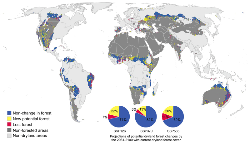
In addition to considering where forests are found today, restoration actions involving tree planting must also consider future climatic conditions, as they will largely determine suitable areas for tree development in drylands, and thus for these actions39. To gain insights about the potential future distribution of dryland forests, we rerun our model for forest extent considering both climatic legacies and projected climate data23 from the MIROC6 global climate model (GCM)40. We used a combination of three Shared Socioeconomic Pathways (SSP) and representative concentration pathways (RCP) scenarios (1-2.6, 3-7.0 and 5-8.5) for these forecasts (see Methods). To obtain a more realistic forecast, we also used projections of the extent of crop and urban land uses in the same three scenarios using the MIROC GCM model27 (see Methods). Our results indicate that about 11% of the current extent of dryland forests (~180 Mha) will be lost in the period 2081-2100 under the SSP5-8.5 projection (Extended Data Fig. 6). At the same time, a total of 309 Mha (20% of the current extent of dryland forest) of new forests will appear in places not holding forests now (Extended Data Fig. 6). Comparing current and potential future forest extent, the areas most affected by forest loss are in eastern Brazil, central Canada, and eastern Australia. The areas projected to have the greatest potential for new forests are in Africa.
In summary, our work provides novel evidence that past climates and aquifer trends are fundamental to explain the current distribution of forests in global drylands and highlights those dryland regions that could foresee future losses and gains of forests under realistic socio-economic and climatic scenarios. The updated estimations of the current and future extension and location of dryland forests provided can be used to improve the management and conservation of forests across drylands worldwide. Our results can also help to prioritize target areas for the establishment of forests in drylands, and to select alternative species (e.g., grasses or shrubs) in areas where future climatic conditions and/or depleted aquifers may not allow the establishment of trees.
Methods
Definition of Forest
We followed the definition of the Food and Agriculture Organisation of the United Nations (FAO), which considers forests as ecosystems with >10% tree cover >5 m in height over 0.5 ha located in areas not predominantly used for agriculture or urban land use41.
Datasets for climatic and other environmental drivers
To delimit the extent of global drylands, we followed the United Nations Convention to Combat Desertification and the Convention on Biological Diversity42, which defined drylands as those areas with an Aridity Index (precipitation/potential evapotranspiration, AI) < 0.65. According to this definition, drylands can be divided into four areas: hyper-arid (AI < 0.05), arid (0.05 ≤ AI < 0.2), semi-arid (0.2 ≤ AI < 0.5), and dry sub-humid (0.5 ≤ AI < 0.65). Here we used the aridity zone map created by the United Nations Environment Programme (UNEP)43.
We used a total of 19 standardized climatic variables in our study (Supplementary Table 1), which were obtained for all the sites surveyed from Worldclim Global Climate Data23. We used data at a 2.5-min resolution (~4.5 km at the equator) because they are available for both the current and past climate of the mid-Holocene (~6000 years ago), so comparisons of bioclimatic data at different periods can be done. We focused on mid-Holocene (i.e., 6000 years before present) climates because many current drylands were wetter during that period31. According to Fick and Hijmans23, the overall accuracy of the Worldclim climatic models was very high for temperature variables. These variables had an overall correlation coefficient (between estimated and observed values) ≥ 0.99 and an average root-mean-square error between 1.1°C and 1.4°C. Precipitation in drylands can be highly variable in time and space, with some regions showing abrupt changes across spatial scales. In general, the prediction error increased with station elevation and distance to the nearest neighbouring station (in the training set) for all variables. Generalized additive models of cross-validation errors showed that higher elevations tended to be associated with lower interpolation accuracy, even after accounting for the effects of isolation and spatial variation in errors, although this effect differed between variables.
We also gathered soil moisture data from TerraClimate44, which is composed of data from Worldclim23 and the Japanese 55-year Reanalysis (JRA55)45; soil organic carbon stock, texture (sand content), and pH from Soilgrids25; albedo from MODIS/Terra MCD43A3 Version 6 product at 500 m pixel resolution46; elevation and slope from the Advanced Land Observation Satellite (ALOS)47; evapotranspiration from MODIS/Terra MOD16A2 Version 6 product at 500 m pixel resolution48; and equivalent liquid water thickness of aquifers by measuring monthly changes in gravity from the Gravity Recovery and Climate Experiment (GRACE)49.
Automatic identification of forest plots
To avoid the low accuracy of classifications using coarse-resolution images13,14 and the subjectivity of using multiple human operators50 we gathered a new high-resolution image dataset and used an automatic classification system to distinguish between forest and non-forest plots based on Convolutional Neural Network (CNN) model, a type of artificial intelligence method inspired by the human brain51. This model can minimise the risk of uncertainty in results but not eliminate it, as the deep learning-based model has been trained with user-provided labels expert in identifying forests in satellite images but is not completely infallible.
We first compiled an updated, globally consistent, and accurate dataset of precise locations of forest and non-forest plots. Based on the valuable information from the 213,795 0.5-ha plots provided by the Global Drylands Assessment13, where 239 operators and FAO staff participated in this task, we selected 94,352 plots where very high-resolution Google Earth images (less than 1 m / pixel, i.e., eye altitude of ~150 m and zoom level 19) were available between 01/Dec/2017 and 13/Dec/2017. Then, the images of these selected plots were automatically classified into forest and non-forest using a CNN-based model.
To train the CNN-based model to differentiate forest from non-forest images, we built a new auxiliary training dataset by regrouping the 45 categories of the NWPU-RESISC45 benchmark database52 (e.g., farmland, forest, mountain, beach, island, lake, river, airport, bridge, church, chaparral, ship) into two classes: forest and non-forest. Our forest class was obtained by grouping together two categories of the NWPU-RESISC45 database: Forest (mainly close forest images) and Chaparral (mainly open forest images). To fulfil FAO’s definition of forest in these classes, we manually removed all images with less than 10% of canopy cover and those including some portion of evident human activity (e.g., infrastructures, tree and non-tree croplands, urban settlements, urban forests, etc.). As a result, our new forest class contained 681 images that fulfilled FAO’s criteria, and our non-forest class contained 30,100 images from all remaining 43 categories of the NWPU-RESISC45 database (e.g., 700 images per category; Supplementary Dataset 1). We used the Inception v.3 architecture53, one of the most accurate CNN models being used nowadays, and two optimization techniques: i) data-augmentation and ii) transfer learning. Data-augmentation consists in artificially increasing the number of independent samples in the training dataset by applying specific transformations to the images (e.g., flipping 180º, margin cropping 10%, scaling up the size of images by 10%, brightening pixel-level up to 50%, and darkening pixel-level up to 50%). Transfer learning consists of using the knowledge acquired from a previous problem to solve a new problem. Instead of starting the learning from scratch, with transfer learning, a pre-trained model is selected and re-trained on the new problem. We used a pre-trained CNN-based model using the ImageNet database54, which contains 1000 image categories including fauna, flora, artificial elements, and other features, with a learning rate of 0.001 and a decay factor of 16 every 30 epochs. As an optimization algorithm, we used RMSProp with momentum and decay of 0.9, and epsilon of 0.1.
Once the CNN-based model was trained, we used it to classify the 94,352 0.5-ha plots described above as forest/non-forest. The CNN-based model analyses each image and outputs two probability values (with their respective confidence intervals), one for the forest class and the other for the non-forest class. To ensure the highest accuracy of the classification (assessed as described below), we removed all plots that were classified by the CNN model with a probability lower than 99%, as well as all plots that had a vegetation height lower than 5m in the Global Vegetation Height dataset28. By doing so, plots with large shrubs would not be counted as forests. Hence, the final dataset used for further analyses contained 16,739 plots with a wide representation along the global drylands (hyper-arid n= 702, arid n= 2883, semi-arid n= 8166, and dry sub-humid areas n= 4988) (Supplementary Dataset 2 and Supplementary Fig. 1).
Assessing the accuracy of the CNN-based model
To assess the accuracy that the CNN-based model had classifying the 94,352 0.5-ha plots of our dataset into forests and non-forests, we randomly selected 705 of these plots and manually checked whether the model properly classified them using Google Earth. These validation plots were selected in a stratified way across the global drylands considering: a) four aridity levels, hyper-arid (AI < 0.05), arid (0.05 ≤ AI < 0.2), semi-arid (0.2 ≤ AI < 0.5), and dry sub-humid (0.5 ≤ AI < 0.65); b) four tree cover levels55: non-forest (<10%), open forest (10-40%), closed forest (41-65%), and dense forest (66-100%); and c) 12 regions13, (Northern Africa; Horn of Africa; The Sahel; Southern Africa; North America; South America (East); South America (West); Central Asia; Southwest Asia; Europe and Russia; Middle East; and Oceania) (Supplementary Table 2). For each combination of aridity level, cover level and region, we randomly selected five images, so the potential number of images would be 4×4×12×5 = 960; however, some strata combinations did not exist. Thus, the total number of images used were 705. The accuracy metrics used were Precision, Recall and the F1-measure (Supplementary Table 3). The F1-measure is an overall score that considers both Precision and Recall and is preferable to simpler methods (F1-measure values close to 1 is better).
Assessing the drivers of current forest distribution
We used variation partitioning56 to quantify the relative importance of bioclimatic variables at different periods and environmental drivers (see Supplementary Table 4) as predictors of the 16,739 forest/non-forest plots previously classified using the CNN model. This method is specifically recommended to deal with multicollinearity because it partitions the variance in a given response variable that is attributed to a particular group of predictors from that variance shared among all predictors. In particular, this analysis provides insights into whether climatic variables from current and mid-Holocene periods can explain a unique portion of the variance that is not explained by climate in other periods56. Variation partitioning analyses were conducted with the R package “Vegan”57.
Importance of the drivers of current forest distribution
We conducted a random forest permutation analysis58 to identify the main predictors of the 16,739 forest/non-forest plots previously classified using the CNN model. Contrary to the variation partitioning model described above, random forest analysis allowed us to identify the most important drivers of forest distribution among 19 bioclimatic variables23 from the different climatic periods studied and other environmental drivers. This method is a novel machine-learning algorithm that extends standard classification and regression tree methods by creating a collection of classification trees with binary divisions. The importance of each predictor variable is determined by evaluating the decrease in prediction accuracy when the data for that predictor is randomly permuted. This decrease is averaged over all trees to produce the final measure of importance. This accuracy importance measure was computed for each tree and averaged over the forest (999 trees). Unlike multimodel inference using linear regressions or regression tree analyses, random forest analysis alleviates multicollinearity problems in multivariate analyses by building bagged tree ensembles and including a random subset of features for each tree (999 trees).
Predicting the extent and distribution of dryland forests
To quantify the global extent and current distribution of dryland forests, we used a random forest regression analysis59 and coupled information on past climates and aquifer trends with other key environmental predictors (e.g., albedo, pH, water thickness, elevation, Precipitation of Warmest Quarter in the current climate, slope, soil moisture, Precipitation of Driest Quarter in the mid-Holocene, Precipitation of Coldest Quarter in the mid-Holocene, Mean Diurnal Range in the current climate; see Supplementary Table 1 and Table 4) that were most important in the permutation analysis58, identifying the main predictors of dryland forest at the 16,739 locations identified by the CNN-based model. This model was built by finding the set of covariate combinations that most robustly predict the training samples and 999 trees. The quality of the classification was tested and validated using a k-fold cross validation method60, where k models (k=5) were trained from k subsets of the original data and tested on k subsets of the remaining independent data (total number of plots divided by k). By combining the k iterations, we compared the original full data set with the full set of the remaining independent data. The modelling approach was then validated by returning the predicted values (x-axis) vs. the observed values (y-axis), following Piñeiro et al.61. The model had a high predictive power (R2=0.89, Supplementary Fig. 2) and the validation of the k-fold cross revealed that our model explained 71% of the variation in forest extent without bias.
To obtain the extent of forests across global drylands, we calculated a map of forest/non-forest areas considering forest as those areas with a probability of being a forest >50% (as provided by the random forest regression analysis). To provide realistic numbers, we eliminated all areas with croplands with at least 60% of the surface and small-scale cultivation mosaics, as well as urban and built-up lands with at least 30% of the surface impervious (including buildings and asphalt) as identified in the global Land Cover Type by Annual International Geosphere-Biosphere Programme (IGBP)26 classification from MOD12Q1 v.6 product by MODIS/Terra satellite sensor62.
Future projections of forest extent in drylands
To calculate future estimates of dryland forest extent globally, we reran our original model, keeping the variables elevation, slope, Precipitation of Driest Quarter in Mid-Holocene, Precipitation of Coldest Quarter in Mid-Holocene while updating the bioclimatic variables Precipitation of Warmest Quarter and Mean Diurnal Range using the estimates provided by the MIROC6 global climate model63. To generate the more reasonable future scenarios63, we chose the combination of three Shared Socio-Economic Pathways (SSP) and representative concentration pathways (RCP) scenarios: 1-2.6, 3-7.0 and 5-8.5 from the Coupled Model Intercomparison Project Phase 5 (CMIP5) over the period 2081-2100. In addition, and to obtain a more realistic extent of dryland forests, we forecasted the extent of agricultural and urban land uses in the same three scenarios using estimations from the MIROC GCM model27. SSP1 is a sustainability scenario, low population growth, high economic growth, high levels of education, good governance, a globalized society, international cooperation, technological development, and environmental awareness. Under these assumptions, this scenario represents low levels of mitigation and adaptation challenges. SSP3 is a fragmentation scenario, high population growth and low economic development, lower levels of education, and a regionalized society with low environmental awareness, thus representing a high level of adaptation and mitigation challenges. SSP5 scenario assumes a very high dependence on fossil fuels, low population growth, high economic growth, and high human development, thus representing a high level of mitigation challenge. The RCP2.6, RCP7.0, and RCP8.5 scenarios consider lower, medium, and high greenhouse gas emission rates (see ref.64 for details).
Uncertainty map
To represent the uncertainty of our predictions of dryland forest extent (Fig. 2), we used the standard deviation of the predictions obtained in the 5-fold cross-validation60 (see the Predicting the extent and distribution of dryland forests section). By stacking the predictions of forest extent, we obtained the mean of the probability to determine the extent of dryland forest and its standard deviation among the five predictive models used. In summary, the standard deviation per pixel, represents the confidence of the model in space (Extended Data Fig. 3). The higher values of this metric, the higher the uncertainty and vice versa.
Consensus and discrepancies between forests areas
We used a simple approach to quantify and locate the consensus between forest maps considering climate legacies and aquifer trends and the forest map created considering only the current climate. The forest consensus is calculated by area Ai, which identifies the i-th pixels of the forest map considering climate legacies and aquifer trends (Forest A), and area Bj, which identifies the j-th pixels of the forest map without considering climate legacies and aquifer trends (Forest B). Then we have the sets of forest areas A = {ai: i = 1, 2, …, m} and B = {bj: j = 1, 2, …, n}. Here, the subscripts i and j are sequential numbers for the pixels of Forest A and Forest B respectively. m and n indicate the total numbers of the pixels of both forest maps. Finally, the corresponding sets of areas of forest A and forest B intersect, obtaining a consensus C between Forest A and Forest B (Equation 1).
| (1) |
Where Cij is the area intersected between the area of map Forest A (areaAi) and the area of map Forest B (areaBj).
This approach generates three types of areas, the intersect of both (Forest A and B) and the exclusive area for each forest map (see Fig. 3).
Paleo-pollen analysis
To check whether trees existed in the locations where dryland forests exist today in the mid-Holocene, we explored data from those sites that are forests today included in the LegacyPollen v.136 database, a harmonization of paleo-pollen databases including a total of 1002 harmonized taxon names. It integrates the Neotoma palaeoecology database (https://www.neotomadb.org/), with additional data65,66. Age data were obtained according to the newly established LegacyAge 1.0 framework67 that includes the mid-Holocene period (5000-7000 Before Present). First, we identified all locations from the LegacyPollen v.1 database that are in areas of current dryland forests. Second, from this subset of dryland locations we identified those pollen samples coming from trees using the GlobalTreeSearch v.1.5 database68, which contains the names of 60,000 tree species. Finally, we summed the percentages of each of the tree pollen samples (n=1121 at 119 sites) and calculated how many samples have 5% or more tree pollen in the mid-Holocene period (Extended Data Fig. 5).
Groundwater balance in forest areas
To identify the extent of forest areas growing over declining aquifers, we calculated the balance (2002-2017) of the accumulated annual equivalent water height (Water Thickness expressed in cm/year) estimated from GRACE49, which has been successfully used to monitor the evolution of the piezometric level of large aquifers based on microgravimetry differences24 (Extended Data Fig. 2). The result of summing monthly values from 2002 to 2017 was classified into three categories: declining (aquifers showing a decrease in their piezometric levels), stable equilibrium (aquifers with unchanged piezometric levels), and increasing (aquifers showing an increase in their piezometric levels).
Extended Data
Extended Data Fig. 1.
Legacies in annual precipitation across global drylands. The bar graphs show the sum of the annual precipitation legacy (precipitation from 6000 years before present minus current precipitation) in dam3 for each aridity level.
Extended Data Fig. 2. Trends (2002-2017) of aquifers located beneath forest areas in drylands.
Extended Data Fig. 3.
Uncertainty map of the current extent of dryland forests. Data based on the standard deviation of predictions obtained from the 5-fold cross-validation (see Methods section).
Extended Data Fig. 4. Comparison of our estimates of forest areas in drylands with recent estimates from the literature15,36.
Extended Data Fig. 5. Results of the analyses of pollen samples of mid-Holocene tree species from the LegacyPollen v.1 database42.
a) Spatial distribution of the studied mid-Holocene pollen samples (n=1121 at 119 sites) overlapping with current dryland forest areas (Figure 2). b) Frequency histogram of the percentage of tree species pollen and its median represented as a dashed vertical line found in the samples per zone. c) Percentage of arboreal pollen found in the samples above 5% in pie charts (top) and Spearman-based correlation of the percentage of arboreal pollen with the aridity index (bottom). Significant in Europe (p-value < 2.2e-16), North America East (p-value = 2.3e-5) and North America West (p-value = 9.6e-12). Shades surrounding the lines represent 95% confidence interval.
Extended Data Fig. 6.
Future changes (potential gains and losses) in dryland forest extent. Data for the 2081-2100 time period according to Shared Socio-economic Pathways (SSP) and representative concentration pathways (RCP) scenarios 1-2.6, 3-7.0 and 5-8.5. Results represented in the map are from the SSP5-RCP8.5 scenarios (see Methods for details).
Supplementary Material
Acknowledgments
We thank Dr. Miguel Berdugo for his advice in the alternative stable states and hysteresis section. We also thank Dr. Blas M. Benito for his advise in the biogeographical analysis of the paleopollen databases. This research was funded by the European Research Council (ERC Grant agreement 647038 [BIODESERT]) and Generalitat Valenciana (CIDEGENT/2018/041). E.G. is supported by the Consellería de Educación, Cultura y Deporte de la Generalitat Valenciana, and the European Social Fund (APOSTD/2021/188). D.A-S. was partially supported by DETECTOR (grant no. A-RNM-256-UGR18, Universidad de Granada/FEDER), LifeWatch SmartEcoMountains (grant no. LifeWatch-2019-10-UGR-01, Ministerio de Ciencia e Innovación/Universidad de Granada/FEDER), RESISTE (grant no. P18-RT-1927, Consejería de Economía, Conocimiento y Universidad from the Junta de Andalucía/FEDER), and EBV–ScaleUp project (funded by Google Earth Engine and the Group on Earth Observations). M.D-B. acknowledges support from the Spanish Ministry of Science and Innovation for the I+D+i project PID2020-115813RA-I00 funded by MCIN/AEI/10.13039/501100011033. M.D-B. is also supported by a project of the Fondo Europeo de Desarrollo Regional (FEDER) and the Consejería de Transformación Económica, Industria, Conocimiento y Universidades of the Junta de Andalucía (FEDER Andalucía 2014-2020 Objetivo temático “01 - Refuerzo de la investigación, el desarrollo tecnológico y la innovación”) associated with the research project P20_00879 (ANDABIOMA). S.T. was supported by DeepL-ISCO (grant no. A-TIC-458-UGR18, Ministerio de Ciencia e Innovación/FEDER), BigDDL-CET (grant no. P18-FR-4961, Proyectos I+D+i Junta de Andalucia 2018) and LifeWatch SmartEcoMountains.
Footnotes
Author Contributions
E.G., M.D.-B. and F.T.M. developed the original idea of the analyses presented in the manuscript. E.G and D.A.-S. develop the global survey. Artificial intelligence analyses were done by E.G. Remote sensing analyses were done by E.G. Statistical modelling, mapping and data interpretations were done by E.G. and M.D-B. The manuscript was written by E.G., F.T.M. and M.D.-B., with contributions from all the co-authors.
Competing interests
The authors declare no competing interests
Data availability
All data generated or analysed during this study, which support the maps within this paper and other findings of this study, are available from Figshare, https://doi.org/10.6084/m9.figshare.13635212.
Code availability
The CNN-based code for classification forest/non-forest described in theMethods is freely available at https://github.com/EGuirado/CNN-Forest-Drylands
References
- 1.Middleton N, Stringer L, Goudie A, Thomas D. The forgotten billion: MDG achievement in the drylands. United Nations Convention to Combat Desertification; Bonn: 2011. [Google Scholar]
- 2.Soong JL, Phillips CL, Ledna C, Koven CD, Torn MS. CMIP5 Models Predict Rapid and Deep Soil Warming Over the 21st Century. Journal of Geophysical Research: Biogeosciences. 2020;125(2) [Google Scholar]
- 3.Huang J, Yu H, Guan X, Wang G, Guo R. Accelerated dryland expansion under climate change. Nat Clim Chang. 2016;6:166–171. [Google Scholar]
- 4.Williams AP, et al. Large contribution from anthropogenic warming to an emerging North American megadrought. Science. 2020;368:314–318. doi: 10.1126/science.aaz9600. [DOI] [PubMed] [Google Scholar]
- 5.Schlaepfer D, Bradford J, Lauenroth W, et al. Climate change reduces extent of temperate drylands and intensifies drought in deep soils. Nat Commun. 2017;8:14196. doi: 10.1038/ncomms14196. [DOI] [PMC free article] [PubMed] [Google Scholar]
- 6.Jiang H. The End of Desertification? Springer; Berlin, Heidelberg: 2016. Taking Down the ‘Great Green Wall’: The Science and Policy Discourse of Desertification and Its Control in China; pp. 513–536. [Google Scholar]
- 7.Gadzama NM. Attenuation of the effects of desertification through sustainable development of Great Green Wall in the Sahel of Africa. World Journal of Science, Technology and Sustainable Development. 2017;14:279–289. [Google Scholar]
- 8.United Nations Decade on Restoration. UN Decade on Restoration. [accessed January 2021]. https://www.decadeonrestoration.org/
- 9.Ellison D, et al. Trees, forests and water: Cool insights for a hot world. Glob Environ Change. 2017;43:51–61. [Google Scholar]
- 10.Feng X, et al. Revegetation in China’s Loess Plateau is approaching sustainable water resource limits. Nat Clim Chang. 2016;6:1019–1022. [Google Scholar]
- 11.Megdal SB. Transboundary Groundwater Resources: Sustainable Management and Conflict Resolution. Groundwater. 2017;55:701–702. [Google Scholar]
- 12.Jarvis WT. In: Advances in Groundwater Governance. Villholth KG, Lopez-Gunn E, Conti K, Garrido A, Van Der Gun J, editors. CRC Press; London, UK: 2017. Cooperation and conflict resolution in groundwater and aquifer management. [Google Scholar]
- 13.Bastin J-F, et al. The extent of forest in dryland biomes. Science. 2017;356:635–638. doi: 10.1126/science.aam6527. [DOI] [PubMed] [Google Scholar]
- 14.Brandt M, et al. An unexpectedly large count of trees in the West African Sahara and Sahel. Nature. 2020;587:78–82. doi: 10.1038/s41586-020-2824-5. [DOI] [PubMed] [Google Scholar]
- 15.Mbow C. The Great Green Wall in the Sahel. Oxford Research Encyclopedia of Climate Science. 2017 doi: 10.1093/acrefore/9780190228620.013.559. [DOI] [Google Scholar]
- 16.Petrie MD, et al. Climate change may restrict dryland forest regeneration in the 21st century. Ecology. 2017;98:1548–1559. doi: 10.1002/ecy.1791. [DOI] [PubMed] [Google Scholar]
- 17.Liu S, Jiang D, Lang X. Mid-Holocene drylands: A multi-model analysis using Paleoclimate Modelling Intercomparison Project Phase III (PMIP3) simulations. The Holocene. 2019;29:1425–1438. [Google Scholar]
- 18.Delgado-Baquerizo M, et al. Palaeoclimate explains a unique proportion of the global variation in soil bacterial communities. Nat Ecol Evol. 2017;1:1339–1347. doi: 10.1038/s41559-017-0259-7. [DOI] [PubMed] [Google Scholar]
- 19.Delgado-Baquerizo M, et al. Effects of climate legacies on above- and belowground community assembly. Glob Chang Biol. 2018;24:4330–4339. doi: 10.1111/gcb.14306. [DOI] [PubMed] [Google Scholar]
- 20.Hoelzmann P, et al. Mid-Holocene land-surface conditions in northern Africa and the Arabian Peninsula: A data set for the analysis of biogeophysical feedbacks in the climate system. Global Biogeochem Cy. 1998;12:35–51. [Google Scholar]
- 21.Fan Y, Li H, Miguez-Macho G. Global patterns of groundwater table depth. Science. 2013;339:940–943. doi: 10.1126/science.1229881. [DOI] [PubMed] [Google Scholar]
- 22.Smettem KRJ, Waring RH, Callow JN, Wilson M, Mu Q. Satellite-derived estimates of forest leaf area index in southwest Western Australia are not tightly coupled to interannual variations in rainfall: implications for groundwater decline in a drying climate. Glob Chang Biol. 2013;19:2401–2412. doi: 10.1111/gcb.12223. [DOI] [PubMed] [Google Scholar]
- 23.Fick SE, Hijmans RJ. Hijmans, WorldClim 2: new 1-km spatial resolution climate surfaces for global land areas. Int J Climatol. 2017;37:4302–4315. [Google Scholar]
- 24.Schmidt R, et al. GRACE observations of changes in continental water storage. Glob Planet Change. 2006;50:112–126. [Google Scholar]
- 25.Hengl T, et al. SoilGrids250m: Global gridded soil information based on machine learning. Plos One. 2017;12:e0169748. doi: 10.1371/journal.pone.0169748. [DOI] [PMC free article] [PubMed] [Google Scholar]
- 26.Friedl MA, Los SO, Brown De Colstoun E, Landis DR, et al. ISLSCP II MODIS (Collection 4) IGBP Land Cover, 2000-2001. ORNL DAAC; Oak Ridge, Tennessee, USA: 2010. [DOI] [Google Scholar]
- 27.Chen M, Vernon CR, Graham NT, et al. Global land use for 2015–2100 at 0.05° resolution under diverse socioeconomic and climate scenarios. Sci Data. 2020;7:320. doi: 10.1038/s41597-020-00669-x. [DOI] [PMC free article] [PubMed] [Google Scholar]
- 28.Los SO. National Centre for Earth Observation. Global Vegetation Height Frequency Distributions from the ICESAT GLAS instrument produced as part of the National Centre for Earth Observation (NCEO) NERC Earth Observation Data Centre; 2015. 10 Dec 2020. http://catalogue.ceda.ac.uk/uuid/85e7d70a74244c73b71446940e05cde6. [Google Scholar]
- 29.Bastin J-F, et al. The global tree restoration potential. Science. 2019;365:76–79. doi: 10.1126/science.aax0848. [DOI] [PubMed] [Google Scholar]
- 30.Cherlet M, et al. World Atlas of Desertification: Rethinking Land Degradation and Sustainable Land Management. Publications Office of the European Union; 2018. [Google Scholar]
- 31.Ganopolski A, Kubatzki C, Claussen M, Brovkin V, Petoukhov V. The influence of vegetation-atmosphere-ocean interaction on climate during the mid-holocene. Science. 1998;280:1916–1919. doi: 10.1126/science.280.5371.1916. [DOI] [PubMed] [Google Scholar]
- 32.Hansen MC, et al. High-Resolution Global Maps of 21st-Century Forest Cover Change. Science. 2013;342:850–853. doi: 10.1126/science.1244693. [DOI] [PubMed] [Google Scholar]
- 33.Scheffer M. tipping points. Princeton University Press; 2009. [Google Scholar]
- 34.Berdugo M, et al. Global ecosystem thresholds driven by aridity. Science. 2020;367:787–790. doi: 10.1126/science.aay5958. [DOI] [PubMed] [Google Scholar]
- 35.Runyan CW, D’Odorico P. Global Deforestation. Cambridge University Press; New York: 2016. p. 248. [Google Scholar]
- 36.Herzschuh U, Böhmer T, Li C, et al. Global taxonomically harmonized pollen data set for Late Quaternary with revised chronologies (LegacyPollen 1.0) PANGAEA. 2021 doi: 10.1594/PANGAEA.929773. [DOI] [Google Scholar]
- 37.Staal A, Fetzer I, Wang-Erlandsson L, et al. Hysteresis of tropical forests in the 21st century. Nat Commun. 2020;11:4978. doi: 10.1038/s41467-020-18728-7. [DOI] [PMC free article] [PubMed] [Google Scholar]
- 38.Belsky AJ, et al. The effects of trees on their physical, chemical and biological environments in a semi-arid savanna in Kenya. J Appl Ecol. 1989:1005–1024. [Google Scholar]
- 39.Li C, Fu B, Wang S, et al. Drivers and impacts of changes in China’s drylands. Nat Rev Earth Environ. 2021;2:858–873. doi: 10.1038/s43017-021-00226-z. [DOI] [Google Scholar]
- 40.Tatebe H, Ogura T, Nitta T, et al. Description and basic evaluation of simulated mean state, internal variability, and climate sensitivity in MIROC6. Geosci Model Dev. 2019;12:2727–2765. doi: 10.5194/gmd-12-2727-2019. [DOI] [Google Scholar]
- 41.Food and Agriculture Organization of the United Nations. Trees, forests and land use in drylands: the first global assessment: Full report. Food & Agriculture Org; 2019. [Google Scholar]
- 42.Diallo HA. In: The Future of Drylands. L C, S T, S, editors. Springer; Dordrecht: 2008. United Nations Convention to Combat Desertification (UNCCD) pp. 13–16. [Google Scholar]
- 43.UNEP-WCMC, A spatial analysis approach to the global delineation of dryland areas of relevance to the CBD Programme of Work on Dry and Subhumid Lands. Dataset based on spatial analysis between WWF terrestrial ecoregions (WWF-US, 2004) and aridity zones (CRU/UEA; UNEPGRID, 1991). Dataset checked and refined to remove many gaps, overlaps and slivers (July 2014)
- 44.Abatzoglou J, et al. TerraClimate, a high-resolution global dataset of monthly climate and climatic water balance from 1958–2015. Sci Data. 2018;5:170191. doi: 10.1038/sdata.2017.191. [DOI] [PMC free article] [PubMed] [Google Scholar]
- 45.Tachikawa T, Hato M, Kaku M, Iwasaki A. Characteristics of ASTER GDEM version 2; 2011 IEEE International Geoscience and Remote Sensing Symposium; 2011. [DOI] [Google Scholar]
- 46.Alibakhshi S, Crowther TW, Naimi B. Land surface black-sky albedo at a fixed solar zenith angle and its relation to forest structure during peak growing season based on remote sensing data. Data Brief. 2020;31:105720. doi: 10.1016/j.dib.2020.105720. [DOI] [PMC free article] [PubMed] [Google Scholar]
- 47.Hamazaki T. Advanced land observation satellite (ALOS). 5 Outline of ALOS satellite system. Journal of the Japan society of photogrammetry and remote sensing. 1999;38:25–26. [Google Scholar]
- 48.Mu Q, Zhao M, Running SW. Improvements to a MODIS global terrestrial evapotranspiration algorithm. Remote Sens Environ. 2011;115:1781–1800. doi: 10.1016/j.rse.2011.02.019. [DOI] [Google Scholar]
- 49.Zlotnicki V, Bettadpur S, Landerer FW, Watkins MM. Gravity Recovery and Climate Experiment (GRACE) gravity recovery and climate experiment (GRACE): Detection of Ice Mass Loss ice ice mass loss, Terrestrial Mass Changes terrestrial mass changes, and Ocean Mass Gains ocean/oceanic mass gains. Encyclopedia of Sustainability Science and Technology. 2012:4563–4584. doi: 10.1007/978-1-4419-0851-3_745. [DOI] [Google Scholar]
- 50.Schepaschenko D, et al. Comment on ‘The extent of forest in dryland biomes’. Science. 2017;358(6362) doi: 10.1126/science.aao0166. [DOI] [PubMed] [Google Scholar]
- 51.LeCun Y, Bengio Y, Hinton G. Deep learning. Nature. 2015;521:436–444. doi: 10.1038/nature14539. [DOI] [PubMed] [Google Scholar]
- 52.Cheng G, Han J, Lu X. Remote Sensing Image Scene Classification: Benchmark and State of the Art. Proc IEEE. 2017;105:1865–1883. [Google Scholar]
- 53.Xia X, Xu C, Nan B. Inception-v3 for flower classification; Proceedings of the 2nd International Conference on Image, Vision and Computing (ICIVC); Chengdu, China. 2–4 June 2017; pp. 783–787. [Google Scholar]
- 54.Fei-Fei L, Deng J, Li K. ImageNet: Constructing a large-scale image database. J Vis. 2010;9:1037 [Google Scholar]
- 55.Guirado E, et al. Tree Cover Estimation in Global Drylands from Space Using Deep Learning. Remote Sens. 2020;12:343 [Google Scholar]
- 56.Legendre P, Borcard D, Roberts DW. Variation partitioning involving orthogonal spatial eigenfunction submodels. Ecology. 2012;93:1234–1240. doi: 10.1890/11-2028.1. [DOI] [PubMed] [Google Scholar]
- 57.Dixon P. VEGAN, a package of R functions for community ecology. Journal of Vegetation Science. 2003;14:927–930. [Google Scholar]
- 58.Breiman L. Random forests. Mach Learn. 2001;45:5–32. [Google Scholar]
- 59.Lahouar A, Slama JBH. Day-ahead load forecast using random forest and expert input selection. Energy Convers Manag. 2015;103:1040–1051. [Google Scholar]
- 60.Kohavi R. A study of cross-validation and bootstrap for accuracy estimation and model selection. Ijcai. 1995;14:1137–1145. [Google Scholar]
- 61.Piñeiro G, Perelman S, Guerschman JP, Paruelo JM. How to evaluate models: Observed vs. predicted or predicted vs. observed? Ecol Model. 2008;216:316–322. [Google Scholar]
- 62.Friedl M, Sulla-Menashe D. MCD12Q1 MODIS/Terra+Aqua Land Cover Type Yearly L3 Global 500m SIN Grid V006. NASA EOSDIS Land Processes DAAC; 2019. distributed by. [DOI] [Google Scholar]
- 63.The CMIP6 landscape. Nat Clim Chang. 2019;9:727. doi: 10.1038/s41558-019-0599-1. [DOI] [Google Scholar]
- 64.Meinshausen M, et al. The RCP greenhouse gas concentrations and their extensions from 1765 to 2300. Clim change. 2011;109(1):213–241. [Google Scholar]
- 65.Cao X, Fang T, Andrei A, et al. A taxonomically harmonized and temporally standardized fossil pollen dataset from Siberia covering the last 40 kyr. Earth Syst Sci Data. 2020;12:119–135. [Google Scholar]
- 66.Cao X, Jian N, Ulrike H, et al. A late Quaternary pollen dataset from eastern continental Asia for vegetation and climate reconstructions: Set up and evaluation. Rev Palaeobot Palynol. 2013;194:21–37. [Google Scholar]
- 67.Li C, Postl A, Böhmer T, et al. Harmonized chronologies of a global late Quaternary pollen dataset (LegacyAge 1.0) PANGAEA. 2021 doi: 10.1594/PANGAEA.933132. [DOI] [Google Scholar]
- 68.BGCI. GlobalTreeSearch online database. Botanic Gardens Conservation International; Richmond, UK: [Accessed on (20/01/2022)]. Available at https://tools.bgci.org/global_tree_search.php. [Google Scholar]
Associated Data
This section collects any data citations, data availability statements, or supplementary materials included in this article.
Supplementary Materials
Data Availability Statement
All data generated or analysed during this study, which support the maps within this paper and other findings of this study, are available from Figshare, https://doi.org/10.6084/m9.figshare.13635212.
The CNN-based code for classification forest/non-forest described in theMethods is freely available at https://github.com/EGuirado/CNN-Forest-Drylands


