Weighted Manifold Alignment using Wave Kernel Signatures for Aligning Medical Image Datasets

Abstract

Manifold alignment (MA) is a technique to map many high-dimensional datasets to one shared low-dimensional space. Here we develop a pipeline for using MA to reconstruct high-resolution medical images. We present two key contributions. First, we develop a novel MA scheme in which each high-dimensional dataset can be differently weighted preventing noisier or less informative data from corrupting the aligned embedding. We find that this generalisation improves performance in our experiments in both supervised and unsupervised MA problems. Second, we use the wave kernel signature as a graph descriptor for the unsupervised MA case finding that it significantly outperforms the current state-of-the-art methods and provides higher quality reconstructed magnetic resonance volumes than existing methods.

1. Introduction

IN many machine learning applications we encounter high-dimensional datasets in which the data lie on a low-dimensional manifold. Manifold learning is a family of machine learning algorithms which aims to find this low-dimensional structure, mapping each high-dimensional point to new coordinates in a low-dimensional space. This mapping ‘unfolds’ the manifold such that, in the new coordinates, the euclidean distance between points can meaningfully describe their similarity. Many approaches have been proposed to solve this problem, including linear methods such as principal component analysis, non-linear spectral methods which can be solved by convex optimisation such as Locally Linear Embedding [19] and Laplacian Eigenmaps [7], and methods requiring non-convex optimisation such as Stochastic Neighbour Embedding [14].

Manifold alignment (MA) is an extension of manifold learning in which two or more datasets are mapped into the same low-dimensional space so that they can be compared directly [13]. MA requires some knowledge of inter-dataset correspondences, which determine which points in different datasets should lie close to each other in the low-dimensional space. In the supervised case these correspondences are given as prior information. In the unsupervised case, they must be derived from the data themselves.

MA has been used in a wide variety of machine learning applications, such as Markov decision processes [23], topical modelling of documents [24], facial recognition [11] and image classification [21].

The alignment of different datasets is a common problem in medical imaging, where two or more datasets may capture the same underlying structure, such as the movement of the body under respiratory motion, but still be difficult to compare directly. These datasets may be different anatomical views, be derived from different imaging protocols [3], [12], [22], or may come from different imaging modalities entirely [2]. By using MA to align these different datasets into a single low-dimensional space, otherwise incomparable medical images can be meaningfully related using their coordinates in the new low-dimensional space [8].

One important application of MA in medical imaging is slice-stacking of magnetic resonance (MR) images, in which dynamically acquired free-breathing high resolution 2D MR slices are retrospectively stacked to form dynamic high-resolution 3D volumes [4]. Although correspondences between the original high-dimensional 2D images are unknown, MA allows these images to be mapped to a common low-dimensional space representing the respiratory motion states at which they were acquired. This allows 2D images from similar motion states to be stacked together into consistent high-resolution 3D images.

Another important application of MA is that of using information from one imaging modality to motion correct another, such as in [2] in which MR imaging was used to correct positron emission tomography (PET) images. In this case MA was used to establish inter-modality data correspondences.

When MA maps different datasets into one common space there is a balance between retaining the structure of each individual dataset, and placing those points with strong inter-dataset correspondences close together, which deforms the shape of the separate datasets’ manifolds. In the existing literature, this deformation of the original manifolds is always bidirectional and uniform, in the sense that the different datasets are equally weighted in the alignment. However, in many cases, such as the medical imaging applications discussed above, the datasets may not be equally informative. Some imaging modalities are noisier than others, and some anatomical views are better at capturing motion information than others. Consequently, it is useful to be able to incorporate this information into the MA scheme, and the development of this methodology is our first contribution here.

As noted above, unsupervised manifold alignment requires correspondences between points in different datasets to be derived from the data. In some cases the datasets are sufficiently similar that these correspondences can be derived by directly comparing each pair of points in the two datasets using, for example, the 𝓁₂ norm [5]. However, there are cases where the data in each dataset are very different and so this type of direct comparison is less meaningful, for example, where the different datasets are medical images containing significantly different anatomy, or come from different imaging modalities entirely. How then should we estimate the inter-dataset similarities when the individual data points cannot be directly compared? One approach is by representing each dataset as a graph, and comparing data points, represented as nodes in the graph, using graph descriptors. If two nodes have similar properties in the graph representation of their respective datasets then they will have similar graph descriptors and so the correspondence between them will be strong. Our second contribution in this paper is to propose the use of the wave kernel signature (WKS) [1] for this purpose. WKS has not previously been used for estimating inter-dataset correspondences for MA, with the exception of our preliminary work in [10].

Combining these two novel contributions we propose a pipeline in which WKS descriptors are used as an input to weighted MA to surpass state-of-the-art performance in aligning medical image datasets.

We will begin with a review of the theory behind our proposed pipeline. The weighted MA principle is demonstrated with simple examples from the COIL-20 image dataset. We then demonstrate our method in three experiments on medical images including both the unsupervised and supervised cases.

2. Theory and Methods

Here we will first review the theory behind manifold alignment, and specifically the method we use here which is based on Laplacian Eigenmaps [7]. We then review the theory behind the use of the WKS graph descriptor for establishing the inter-dataset correspondences in the unsupervised case.

2.1. Manifold Alignment

Manifold learning is a tool for non-linear dimensionality reduction which aims to extract low dimensional manifolds from high-dimensional datasets. We denote the high-dimensional data by X = [x₁, x₂, … x_T], which consists of T points in ℝ^D. In general, the dimensionality D may be very large, for example, the number of pixels in an image. Assuming that the points in X each lie on or close to a manifold ℳ of dimension d, manifold learning constructs a map from ℝ^T×D to ℝ^T×d where d ≪ D. The result is a new low-dimensional dataset, Y = [y₁, y₂, …, y_T] which describes each point’s position on ℳ.

Manifold learning techniques which work by optimising a cost function can be extended to perform manifold alignment by adding terms to their cost function which represent inter-dataset alignment [13]. Here we briefly review how Laplacian Eigenmaps can be extended to perform manifold alignment.

The Laplacian Eigenmaps algorithm involves first forming a graph 𝒢 where each datapoint i has an edge with its k_𝒢 nearest-neighbours, the set of which is denoted by η_i. The edge between points i and j is weighted by:

$$W_{ij}=\{\begin{array}{cc}\text{exp}\left[\frac{-\parallel x_i-x_j{\parallel }^2}{2{\sigma }_{𝒢}^2}\right]& \text{if}j\in {\eta }_i\\ 0& \text{otherwise},\end{array}$$ (1)

where σ_𝒢 is a parameter which determines the strength of neighbourhood relations. Since the nearest-neighbour relation is not necessarily symmetric we symmetrise the adjacency matrix W, whose elements are given by $W_{[i,j]}=\frac{1}{2}\left(W_{ij}+W_{ji}\right)$. The cost term we seek to minimise is given by

$$\text{Φ}\left(\mathbf{\text{Y}}\right)=\frac{1}{2}{\displaystyle \sum _{i,j}{\mathbf{\text{W}}}_{[i,j]}{\Vert {\mathbf{y}}_i-{\mathbf{y}}_j\Vert }^2},$$ (2)

subject to the constraint that Y^TDY = I, where D is the diagonal degree matrix D_[i,i] = Σ_j W_[i,j]. Minimising Φ(Y) forces points with highly weighted connections to be close to each other, while the constraint prevents all coordinates collapsing onto a single point. This cost term can be rewritten as

$$\text{Φ}(Y)=\text{tr}\left(Y^{T}LY\right),$$ (3)

where the graph Laplacian, L is the matrix given by

$$L=D-W.$$ (4)

Note that, since the product in Equation (3) of L with the low-dimensional coordinates Y is equal to the cost term in Equation (2) which must be non-negative, L is positive semi-definite and therefore has no negative eigen-values. As shown in [7] Equation (3) is minimised by the eigenvectors of L corresponding to the d smallest non-zero eigenvalues, and so these provide the desired low-dimensional coordinates Y.

MA is achieved by extending this formulation to the case of N high-dimensional datasets. The joint cost term becomes

$${\text{Φ}}_{\text{total}}={\displaystyle \sum }_{\ell }{\text{Φ}}^{(\ell )}+\frac{\mu }{2}{\displaystyle \sum }_{\begin{array}{c}n,m\\ n\ne m\end{array}}{\displaystyle \sum }_{i,j}{U}_{[i,j]}^{(n,m)}\parallel y_i^{(n)}-y_j^{(m)}{\parallel }^2,$$ (5)

where Φ^(𝓁) is the cost term for each individual dataset, U^(n,m) is some similarity kernel between datasets X⁽ⁿ⁾ and X^(m), and μ is the parameter that weights the intra-dataset terms versus the inter-dataset terms. The values of the matrices U^(n,m) determine which points in datasets n and m should be placed close together in the aligned manifold.

We assume that the matrices U have the symmetry $U_{[i,j]}^{(n,m)}=U_{[j,i]}^{(m,n)}$. The total cost Φ_total(Y) is, as above, minimised by

$${\text{Φ}}_{\text{total}}(Y)=\text{tr}\left(Y^{T}MY\right),$$ (6)

where Y denotes the low-dimensional coordinates for each dataset concatenated together, and M is the block matrix of inter-dataset and intra-dataset terms given by

$$M=\left[\begin{array}{cccc}{L}^{(1)}+\mu D^{(1)}& -\mu U^{(1,2)}& \dots & -\mu U^{(1,N)}\\ -\mu U^{(2,1)}& L^{(2)}+\mu D^{(2)}& \dots & -\mu U^{(2,N)}\\ ⋮& ⋮& \ddots & ⋮\\ -\mu U^{(N,1)}& -\mu U^{(N,2)}& \dots & L^{(N)}+\mu D^{(N)}\end{array}\right],$$ (7)

$$D_{[i,i]}^{(\ell )}={\displaystyle \sum }_{\ell \ne n}{\displaystyle \sum }_j{U}_{[i,j]}^{(\ell ,n)}.$$ (8)

As before, this cost is minimised by the eigenvectors of M corresponding to the smallest non-zero eigenvalues.

2.2. Weighted Manifold Alignment

The joint cost function in Equation (5) balances terms that maintain the structure of each individual dataset’s manifold (the Φ^(𝓁) terms) and those aligning datasets to each other (the terms containing U). The parameter μ determines the relative strength of these two forces. This formulation implicitly assumes that the structure of each manifold ought to be maintained to the same degree. The first novel part of our pipeline is to introduce a term to weight each dataset and its relationship to the others as follows, generalising Equation (5) to:

$${\text{Φ}}_{\text{total}}={\displaystyle \sum }_{\ell }{c}_{\ell }^2{\text{Φ}}^{(\ell )}+\frac{\mu }{2}{\displaystyle \sum }_{\begin{array}{c}n,m\\ n\ne m\end{array}}{\displaystyle \sum }_{i,j}{c}_n{c}_m{U}_{[i,j]}^{(n,m)}\parallel y_i^{(n)}-y_j^{(m)}{\parallel }^2,$$ (9)

where {c_𝓁} is the set of weights. If, as in [16], we imagine the manifolds for each dataset as points connected by springs with a rest length of 0, increasing c_𝓁 increases the rigidity of manifold Y^𝓁 by proportionally increasing the spring constants, and similarly forces other manifolds to deform to more closely fit the shape of Y^𝓁. Therefore this formulation allows us to use information about the relative rigidities we would like to assign to the manifolds representing each dataset. To perform the embedding we then find the eigen-vectors of the weighted matrix:

$$M_{\text{w}}=CMC,$$ (10)

where C is the diagonal matrix of weights c_𝓁. The question of how these weights ought to be derived is one which will depend on the application at hand and what prior information is available to suggest that one dataset should be prioritised over another. We return to this question in Section 3.2.

2.3. Graph Descriptors

In unsupervised MA the inter-dataset similarities U must be derived from the data. The methods assessed here use graph descriptors to compare points in each dataset. For each dataset, a graph 𝒢 is constructed with edges weighted by parameter σ_𝒢 as in Equation (1). Descriptors are then computed for each node in each graph and compared to determine the matrices U^(n,m). Note that this formulation assumes that the graphs describing each dataset are sufficiently similar to each other to allow an unsupervised comparison but that this is a looser assumption than that made by methods which directly compare data from different datasets such as in [5].

The WKS [1] is part of a family of graph methods which use the eigenvectors of the graph’s Laplacian to compare vertices. The graph Laplacian, L, can be interpreted as a discrete version of the Laplace-Beltrami operator and so can be used to describe diffusive processes on the graph [7]. We denote the Laplacian’s eigenvalues as E_k and eigenvectors as v_k. The WKS is a function ω_i (z) for each node i in the graph, defined as

$${\omega }_i(z)=B(z){\displaystyle \sum }_k{v}_{k,i}^2\exp \left[\frac{-{(z-\log \left(E_k\right))}^2}{2{\sigma }_{\omega }^2}\right],$$ (11)

where B(z) is a normalisation term given by

$$B(z)={\left({\displaystyle \sum }_k\exp \left[\frac{-\left(z-\log \left(E_k\right)\right)}{2{\sigma }_{\omega }^2}\right]\right)}^{-1}.$$ (12)

This function is a stable and highly informative descriptor [15] which corresponds to the diffusion of a quantum mechanical particle of energy z on the graph [1]. The parameter σ_ω is a measure of the ‘smoothness’ of this descriptor which is normally constant and manually chosen for the task at hand.

The similarity between two nodes, i and j in the two graphs n and m can be assessed by measuring a distance, ${\text{Δ}}_{ij}^{(n,m)}$, between their wave kernel signatures, where

$${\text{Δ}}_{ij}^{(n,m)}={{\displaystyle \int }}_{z_{\min }}^{z_{\max }}\frac{{\omega }_i^{(n)}(z)-{\omega }_j^{(m)}(z)}{{\omega }_i^{(n)}(z)+{\omega }_j^{(m)}(z)}dz.$$ (13)

The similarity kernels are then given by

$$U_{[i,j]}^{(n,m)}=\exp \left[\frac{-{\left({\text{Δ}}_{ij}^{(n,m)}\right)}^2}{2{\sigma }_{\text{WKS}}^2}\right],$$ (14)

which ensures that vertices with similar wave kernel signatures have a high similarity in U. We set σ_WKS = 1 for our experiments using unsupervised MA.

As in [3], once a descriptor has been used to generate a similarity kernel U^(n,m), the kernel is then sparsified by using the Hungarian algorithm to establish one-to-one correspondences with maximal similarity and it is these sparsified kernels that are used for MA.

3. Experiments

We begin by illustrating the weighted MA method in the supervised case with a simple toy experiment using the COIL-20 dataset of images of small objects. Next we demonstrate our full pipeline using the WKS descriptors in three experiments using medical images. First, slice-stacking of highly realistic synthetic MR data for which we have a ground truth to quantitatively compare the quality of the reconstructed volumes. Second, slice-stacking of real MR data gathered from 8 healthy subjects, where we measure the self-consistency of the reconstructed volumes. These two experiments both demonstrate the unsupervised case. Third, we demonstrate semi-supervised MA on simultaneously acquired PET and MR images, where we measure the ability of the low-dimensional embedding to recover a respiratory signal from the low signal-to-noise ratio PET data using MA with higher quality MR images.

3.1. Supervised MA Using a Toy Model: COIL-20 Dataset

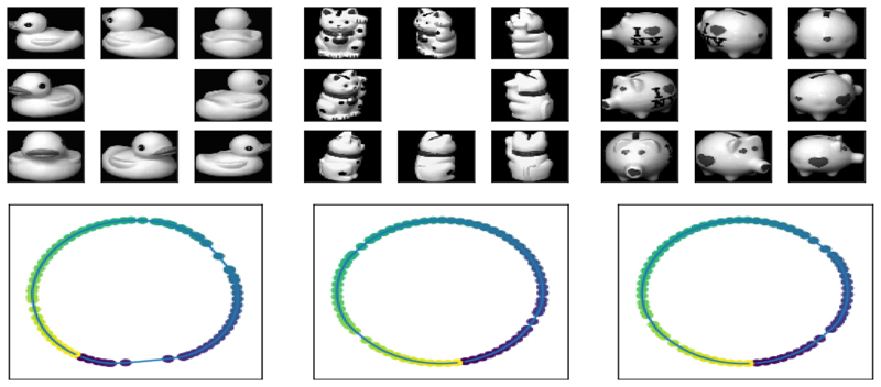
Here we demonstrate the idea of weighted MA with some simple examples from the COIL-20 dataset of small objects photographed from different views [18]. Each object is photographed from 72 different angles which form a full rotation around the object, such as in the examples shown in Fig. 1. Performing dimensionality reduction on each set of images unsurprisingly reveals that the images lie on a topologically circular manifold, representing the path taken by the camera taking the images (see Fig. 1).

Fig. 1.

Top: Example images of a toy duck, cat and pig from the COIL-20 dataset. Each object is imaged 72 times under one full rotation and images are 128 × 128 pixels. Bottom: Laplacian eigenmaps embedding for these three datasets (from left to right, the duck, cat and pig), with k_𝒢 = 4. The colour of each point corresponds to the viewing angle.

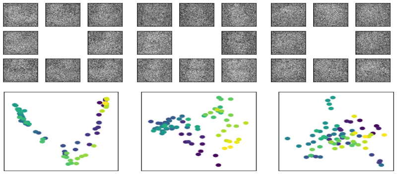
To demonstrate weighted MA in a simple context we find the joint embedding of three of these datasets in a supervised manner, where correspondences between the datasets are determined by the angle the images were taken from, meaning that the matrix U is the identity matrix (i.e., no graph descriptors are used). We perturb two sets of images with Gaussian noise (mean 0 and standard deviation 1 where the original images’ pixel intensities range from 0 to 1), as shown in Fig. 2, which in turn affects the low-dimensional embedding.

Fig. 2.

Top: The same example images from the COIL-20 dataset with significant Gaussian noise added (standard deviation of 1 where the original image pixel intensities are normalised between 0 and 1). EachBottom: Laplacian eigenmap embeddings for these datasets, with k_𝒢 = 4. Some of the structure seen in Fig. 1 is present but much has been lost.

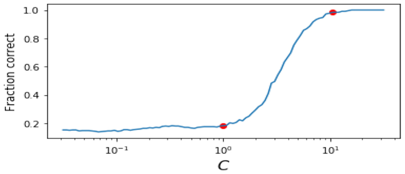
However, by weighting more heavily the set of images without noise than those with the noise we can fit the noisy dataset to the clean dataset, demonstrating how weighted MA can allow for asymmetry in the alignment step, favouring one dataset over the other. Fig. 3 shows the standard MA and three different weighted MA embeddings. We can see that more heavily weighting the clean dataset produces embeddings which appear more similar to those in Fig. 1 than is the case when the noisy datasets are weighted more heavily, or when there is no weighting at all (i.e., standard MA). We quantify this improvement by counting the fraction of points in the noisy dataset whose nearest neighbour in the aligned embedding is the correct nearest neighbour from the original dataset. Fig. 4 shows these results. Here the weights were c_𝓁 = 1 for the noisy dataset, and c_𝓁 = C for the noiseless dataset. As expected, when the weighting on the noiseless dataset is high this fraction is close to one, as the original structure is recovered. When the weighting on the noisy dataset is high it is close to zero, as the noise in the noisy datasets dominates. Note that the standard unweighted case, at the highlighted point in Fig. 4 where C = 1, performs significantly worse than the weighted case here. This is because without any weighting the noiseless manifold and noisy manifold both deform so as to align in the low-dimensional space. Weighting the noiseless dataset’s contribution more makes that manifold more rigid, forcing the noisy manifold to deform to match. We will now use this idea of weighting some datasets in the MA step in experiments on medical image alignment.

Fig. 3. Joint embeddings, using weighted MA of the three sets of images, where the noiseless dataset is used for the images of the duck, but the noisy data used for the cat and pig images.

In all cases we show all three datasets’ embedding together. Left: Applying no weighting (standard MA). Centre left: Weighting the noisy cat images by a factor of 10. Centre right: Weighting the noisy pig images by a factor of 10. Right: Weighting the noiseless duck images by a factor of 10. It is clear that only in the final case, where the noiseless dataset is weighted, is the original manifold structure cleanly recovered. The idea behind our MA scheme is that it produces joint embeddings like that on the right of this figure rather than like those on the left.

Fig. 4. The fraction of nearest neighbours correctly predicted by the results of the MA plotted against the weighting applied to the noiseless dataset.

As the weighting C increases the fraction of correct predictions goes to 1. Note that the unweighted case, C = 1, highlighted by the red marker performs significantly worse than the strongly weighted case highlighted at C =10.

3.2. Unsupervised Alignment of Synthetic MR Volumes

In this experiment we demonstrate that weighted MA, using the WKS to estimate the inter-dataset correspondence, provides state-of-the-art performance on the problem of MR slice stacking. The MR slice stacking problem can be stated as follows: we are given a series of T high resolution 2D images for each of N sagittal slices with each image labelled $x_t^{(n)}$ where t ∈ {1, 2, …, T } and n ∈ {1, 2, …, N}. In general, the images are taken at different times and so there are no prior correspondences between them. It is these correspondences which must be found in an unsupervised manner. Our aim is to take one of the sagittal slices, n*, and for each of the T images in that sequence, reconstruct a volume $V_t^{\left(n^{\ast }\right)}$ around it by choosing an image from each of the other N − 1 slices which is in the same motion state as $x_t^{\left(n^{\ast }\right)}$ and then stacking them together. This produces a dynamic sequence of 3D volumes capturing the motion of interest, which is clinically useful as the acquired 2D images can have much higher spatial resolution and better contrast than dynamically acquired 3D volumes.

This experiment uses synthetic data in which we start with synthetic high-resolution 3D volumes, so that the reconstructed images can be compared to this ground truth. This synthetic dataset is highly realistic, and is based on image registration of a real respiratory-gated high spatial resolution 3D MR volume to a series of real dynamic 3D low spatial resolution MR volumes. The high resolution volume was warped using the registration results to create a series of realistic high spatial resolution volumes at different respiratory motion states. We use a sequence of T = 250 volumes each with N = 40 sagittal slices. The generation of this dataset is described in full detail in [9].

We use MA to generate a low-dimensional manifold containing T × N points, labelled $y_t^{(n)}$, with each point representing the image $x_t^{(n)}$. We then choose a slice, n*, around which to reconstruct a volume. For each image $x_t^{\left(n^{\ast }\right)}$ in this slice, and each other slice m ≠ n*, we find the s ≠ t that minimises $\parallel y_t^{\left(n^{\ast }\right)}-y_s^{(m)}{\parallel }^2$ and stack these $x_s^{(m)}$ together into a 3D volume in which each slice should be at a consistent motion state with the initial image $x_t^{\left(n^{\ast }\right)}$. We then compute an error on the reconstructed volumes, $V_t^{\left(n^{\ast }\right)}$ by comparing them to the original ground truth volumes.

Note that the restriction that s ≠ t is required for this experiment as the data used are synthetic 3D volumes and so slices acquired at the same time would necessarily have the same motion state and so give artificially accurate reconstructed volumes. Similarly, when sparsifiying the matrices U with the Hungarian algorithm in this experiment we do not allow a datapoint in one dataset to be matched with the datapoint in another dataset if it shares the same time index. This restriction does not need to be made in cases where the data consist of 2D slices, as in the clinically relevant case (see Section 3.3).

The error for a reconstructed volume is given as the mean of the squared error in image intensities, and we report the median error over the N slices used for the reconstruction, since the error distribution over the slices is skewed. In our preliminary version of this work, [10] we found that in this experiment the WKS was more effective than other graph descriptor methods. Here we show that using weighted MA can provide further improvements.

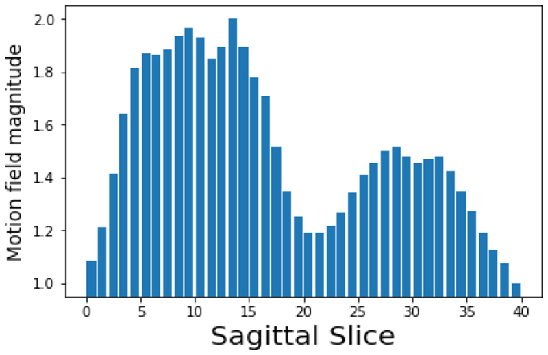
As discussed in Section 2.2 and the toy experiment in Section 3.1, it may be possible to improve the MA step in our pipeline by more heavily weighting certain datasets (in this case, certain sagittal slices) which are more informative than others. Here, we are trying to align slices such that they have consistent motion states with regard to respiratory motion. Therefore, we choose to weight those slices in which respiratory motion is most pronounced so that different respiratory states may be more clearly distinguished. To do this we perform image registration on each slice’s set of images (using the package NiftyReg [17]) to extract a motion field for each time-step. For each slice we then find the variance of the magnitude of the motion field vectors over all timesteps, and use this value as an estimate of the extent of respiratory motion in that slice. Fig. 5 shows this respiratory motion magnitude for each sagittal slice, illustrating that it is those slices in the centre of the lungs which have the most pronounced motion, which is consistent with clinical knowledge of respiratory mechanics.

Fig. 5. Normalised motion field magnitude for each sagittal slice in the high-resolution dynamic synthetic MR volumes.

The two peaks correspond to the slices through the left and right lungs, and the right lung shows more significant motion due to the heart obscuring the left lung (as in the images in Fig. 9 the volunteer’s right lung corresponds to the left of the image). Using these values as the dataset weights c_n will place more emphasis on the sagittal slices in the centre of the lungs, rather than those around the edge of the torso or around the spine. Here the weights are normalised to have a maximal value of C = 2 and a minimum of 1.

We compare our proposed pipeline of WKS and weighted MA with the unweighted case, and with weighted MA using two other graph descriptors; the random walk (RW) feature vector as used for slice stacking in [6], [9] and the commonly used heat kernel signature (HKS) [20]. In both of these alternative methods the similarity kernel is also sparsified with the Hungarian algorithm.

The random walk method involves constructing a vector π for each node in which component π_r describes the probability of a random walker on the graph being found within the r nearest neighbours of the node. These vectors are then compared by computing the euclidean difference between them, and similarities computed with a Gaussian kernel parametrised by a width σ_RW.

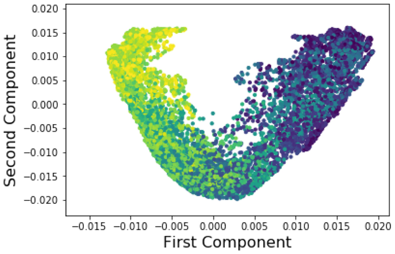
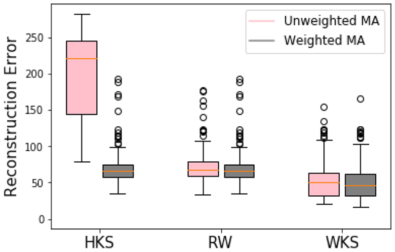
The heat kernel signature descriptor is similar to the WKS but differs in that the exponential term in (11) and (12) is replaced with exp[−E_kz], with the matrices U calculated as in Equation (14) with a free parameter σ_HKS which is analogous to σ_WKS. The parameters used here, found by grid-search, were σ_𝒢 = 1.5 for the construction of the graphs used, for the wave kernel signature method σ_ω = 0.8, σ_WKS = 1, for the heat kernel signature method σ_HKS = 1 and for the random walk method σ_RW = 0.02 and for the MA step k_𝒢 = 15, σ_𝒢 = 10. and µ = 0.05. A sample embedding produced by MA using the WKS descriptor is shown in Fig. 6. The 250 error values computed as described above are plotted for each method in Fig. 7. Using a two-tailed Wilcoxon signed rank test we found statistical significance with p < 0.01 that the weighted MA method with the WKS graph descriptor outperformed the other assessed methods. In this experiment the manifold weights were normalised with a minimum of 1 and maximum of 2, although the method is robust to changes in this maximal value as discussed in Section 4.

Fig. 6. An example of the low-dimensional embedding generated from the WKS graph descriptor and weighted MA.

All sagittal slices are shown. Colour corresponds to a respiratory navigator generated from the gold standard synthetic images. The ’v’ shape of the manifold is typical, but the strong relation between the position in the manifold and the colour of the points illustrates that the embedding places close together points which share similar respiratory motion states, as intended.

Fig. 7. Mean square difference between reconstructed volumes and ground truth volumes using the proposed wave kernel signature (WKS) graph descriptor, and the heat kernel signature (HKS) and random walk (RW) feature vector descriptors.

For each method 250 values are generated, one for each timestep of the synthetic 4D volumes. Volumes are reconstructed using every sagittal slice and the median error taken, which is shown here. The proposed weighted MA scheme reduces the reconstruction errors in each case, and the WKS + weighted MA pipeline gives the lowest error.

3.3. Unsupervised Alignment of Real MR Slices

In this experiment we demonstrate the use of MA for slice-stacking on real MR data acquired from 8 healthy volunteers. Each dataset has a field of view covering the entire thorax, including the lungs and liver. The data consist of N sagittal slices of thickness 8 mm, where N is typically around 35. The 2D images were acquired by taking one image from each slice position, iterating through the slices one by one, and then repeating this process until 40 images were obtained for each slice position, the same protocol as used in [5]. For volunteers A-D one image was acquired per heartbeat (at systole) so as to isolate respiratory motion, and for volunteers E-H there was no such cardiac gating. The acquisitions were carried out on a Philips Achieva 3T MR scanner using a T1-weighted gradient echo sequence with an acquired in-plane image resolution of 1.4 × 1.4 mm², a slice thickness of 8 mm, repetition and echo times (TR and TE) of 3.1 and 1.9 ms, a flip angle of 30 degrees, and a SENSE-factor of 2. The field of view covering the entire thorax was 400 × 370 mm², and each slice took around 180 ms to acquire.

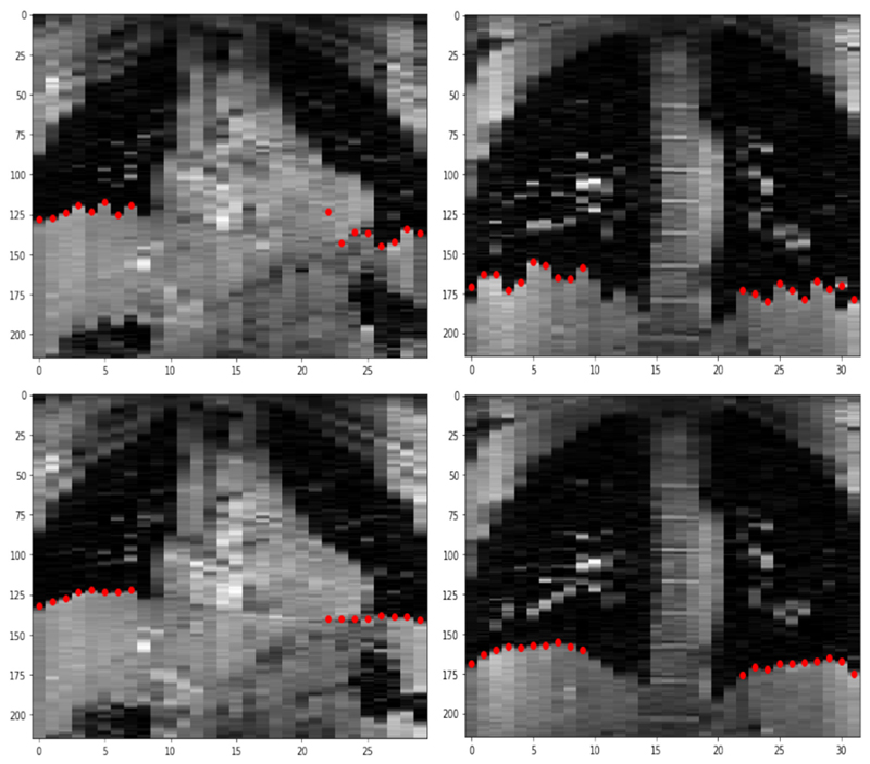
This experiment was performed similarly to that in Section 3.2 except that it resembles the slice-stacking problem in a clinical setting and so there is no ground truth volume to compare the reconstructed volume against. We therefore quantify the consistency of the reconstructed volumes by measuring the correlation of the positions of the left and right hemidiaphragms [3]. Volumes are reconstructed from the aligned manifolds as in the experiment in Section 3.2. For each volunteer, a coronal slice in which the diaphragm is visible is selected and within that coronal slice the diaphragm position in each 1D sagittal slice is automatically identified by finding the point with the greatest difference in image intensity within a manually delineated box on the inferior lung boundary. Fig. 8 shows such coronal slices from the raw data in which the sagittal slices are in different motion states, and from reconstructed volumes for two volunteers with the diaphragm positions marked. We quantify the consistency of these volumes by measuring the correlation between the diaphragm positions in the left and right hemidiaphragms - i.e., the left set of markers and right set of markers in the images in Fig. 8. If the volumes are reconstructed successfully then all sagittal slices will share respiratory states and so these markers will move up and down synchronously, giving a high measured correlation. We find that our pipeline reconstructs volumes with the highest such correlation of the methods we test, as shown in Table 1.

Fig. 8.

Top: Examples from volunteers A (left) and D (right) of a coronal slice through the original unaligned volumes. The sagittal slices are not in consistent motion states resulting in discontinuities in diaphragm positions. Bottom: Examples from a volume reconstructed by stacking sagittal slices aligned by motion state. Estimated diaphragm positions for left and right lungs are shown in red.

Table 1. Pearson’s Correlation Coefficient between Left and Right Hemidiaphragm Positions of Reconstructed Volumes.

Volunteer	Method	Hemidiaphragm correlation
		WKS	HKS	RW
A	MA	0.957	0.400	0.794
	Weighted MA	0.967	0.660	0.774
B	MA	0.868	0.393	0.720
	Weighted MA	0.935	0.515	0.657
C	MA	0.873	0.460	0.649
	Weighted MA	0.924	0.586	0.678
D	MA	0.756	0.814	0.691
	Weighted MA	0.897	0.833	0.695
E	MA	0.640	0.455	0.426
	Weighted MA	0.739	0.658	0.494
F	MA	0.613	0.312	0.250
	Weighted MA	0.775	0.512	0.431
G	MA	0.512	0.199	0.304
	Weighted MA	0.820	0.358	0.541
H	MA	0.470	0.278	0.462
	Weighted MA	0.698	0.380	0.505

A volume can be reconstructed from each sagittal slice, each giving its own correlation coefficient over all time points; here we report the median across these slices. The best result for each volunteer is shown in bold. The cardiac gating for the acquisition of data for volunteers A-D results in more accurately reconstructed volumes than is the case for E-H, but in both cases the weighted MA scheme is beneficial.

3.4. Semi-Supervised Alignment of MR and PET

This experiment demonstrates weighted MA in the semi-supervised case. We aim to mimic a realistic simultaneous PET-MR scanning scenario in which paired PET and MR data are acquired continuously, but with short gaps in MR data acquisition representing scan sequence planning [2].

The task is as follows: we have a sequence of N_𝓁 3D MR volumes, each volume coming with an associated PET sinogram with which it was simultaneously acquired (these are the labelled PET sinograms). We then have a further N_u PET sinograms with no corresponding MR volumes (these are the unlabelled PET sinograms). Each sinogram also has an associated respiratory navigator which is a 1D signal, which we consider to represent the ground truth respiratory state. The task is to estimate the respiratory navigator for the unlabelled sinograms by using semi-supervised MA to align the high quality MR data with PET data which have a low signal-to-noise ratio. Since known correspondences exist for the labelled data there is no requirement for an inter-dataset correspondence step and so we can directly analyse the effect of changing the relative weights of each dataset’s contribution to the MA loss function. Our interdataset correspondence matrix U is then a (N_𝓁 + N_u) × N_𝓁 matrix with 1 on the diagonal and zeros in the rows corresponding to the unlabelled points as in [2].

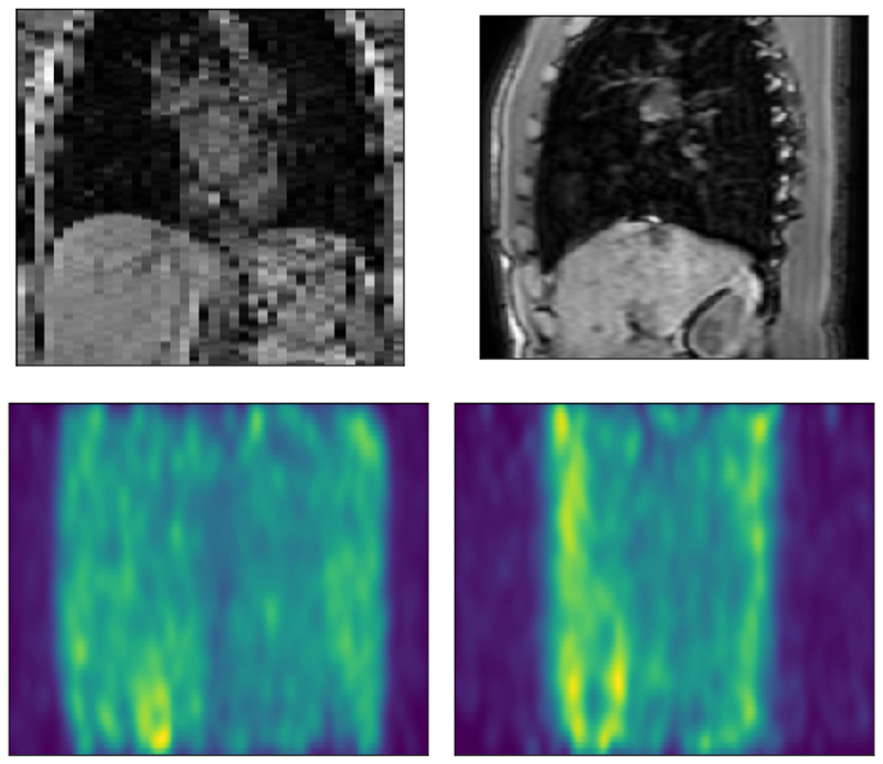
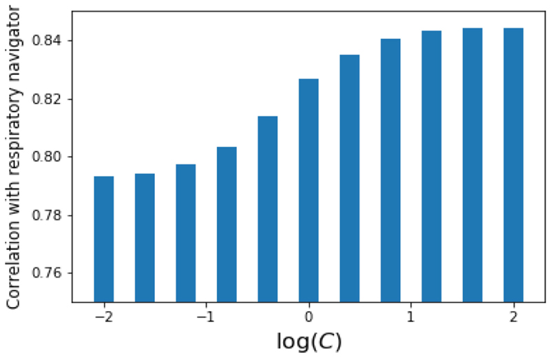
Our MR volumes are the same as those described in Section 3.2. The PET data are synthetically generated as described in [9], and we use N_𝓁 = 450 and N_u = 50 for a total of 500 PET sinograms. Examples of the high-quality MR images and the low signal-to-noise ratio PET views are given in Fig. 9. Fig. 10 shows the effect of varying the weight, C of the MR data in this semi-supervised MA approach on the correlation of the low-dimensional coordinates of the unlabelled PET data, with the ground-truth respiratory signal. The weight of the PET data is set to 1. We see that weighting more heavily the high-quality MR images forces the labelled PET data to align to the MR data, and the intra-dataset relations between the labelled and unlabelled PET data then fit the unlabelled PET points to this high quality signal. As a result, we see that the correlation with the respiratory signal increases when this weight is increased.

Fig. 9.

Top: A coronal and sagittal view of the synthetic MR volumes. Bottom: corresponding projections of a PET sinogram, which is visibly noisier than the MR image due to the stochastic nature of this imaging modality.

Fig. 10. Correlation between low-dimensional coordinates of unlabelled PET data and ground truth respiratory signal as a function of manifold weighting on the MR data with which the labelled PET sinograms are aligned.

Heavily weighting the MR images results in an embedding which more closely corresponds with respiratory motion state.

4. Discussion and Conclusions

In the preliminary version of this work [10] we found that using the WKS descriptor gave state-of-the-art performance for the MR slice stacking problem. Here, we have extended that work by developing the novel technique of weighted MA, which yields further improvements in the quality and consistency of reconstructed volumes.

The weighted MA scheme is a generalisation of MA techniques in the sense that in previous work, the parameter we call µ, which sets the relative strength of the inter-manifold and intra-manifold forces was constant across every pair of inter-manifold comparisons. There are cases where this is appropriate, and if no prior reason exists to weight one dataset more heavily than another then assuming uniform weights is the most reasonable option. But there are numerous applications where this kind of prior information is available and to not use it is to sacrifice performance in solving the MA problem. Here we have shown two domains in medical imaging in which this prior knowledge is useful. First, that sagittal MR slices with more significant motion can be more useful for matching images with consistent motion states. Second, that imaging modalities with low signal-to-noise ratio (e.g., PET) can be fitted to modalities with higher signal-to-noise ratio (e.g., MR).

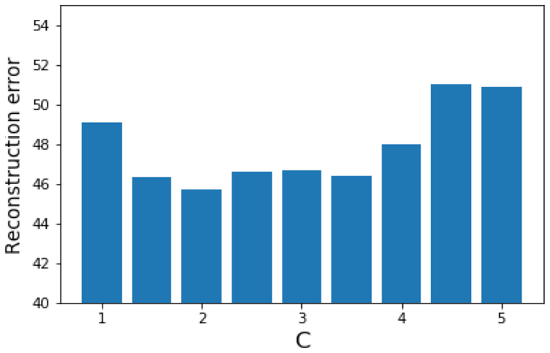
The question of how to optimise the manifold weights remains a largely open one which is dependent on the application at hand. In the simple example given in Section 3.1 we see that arbitrarily high weights are optimal, but this is just a consequence of the experimental set-up in which we know with certainty that one dataset is completely noiseless. In more complex, realistic applications such as in Section 3.2 this is no longer the case. We used the magnitude of the respiratory motion fields to determine which sagittal slices were most informative, and in our experiment normalised the maximum weight assigned. Unlike in the toy experiment it is not the case though that increasing this constant will always increase performance. Fig. 11 shows that a range of optimal weight values exist beyond which performance degrades again.

Fig. 11. The reconstruction error for the WKS method in the experiment described in Section 3.2 as function of the maximum manifold weight.

As described in that experiment using a weight larger than 1 reduces reconstruction error, but setting the weight too high degrades performance.

In our preliminary work [10] we used a novel graph descriptor we called the adaptive WKS. This graph descriptor uses the difference between the sequence of eigenvalues of two graph Laplacians to set the parameter σ_ω in the WKS descriptor. This method provided statistically significant improvements over the standard WKS descriptor in the experiments in that paper, which are similar to those presented in Sections 3.2 and 3.3 here. We found that using the weighted MA step presented here was a more effective way of incorporating prior knowledge about the reliability of information in different datasets, but that combining the two methods did not improve performance (although it does incur a computational cost). We explain this by noting that these changes are both motivated by the same intuition - that some datasets in the MA step should be considered more informative than others. In the adaptive WKS this takes the form of matching more informative (i.e., central lung sagittal slices) and less informative slices taking into account that they are dissimilar, but not in a way which specifies which of the two is the informative one. In the weighted MA this takes the form of asymmetrically fitting the less informative dataset to the informative dataset by assigning different values of the manifold weights c_𝓁 in Equation (9) - asymmetric in that the cost term for deforming the manifold structure of the highly weighted dataset is larger. When reliable information about which dataset should be considered more informative is available, the latter method accounts for this information better and thus produced dynamic MR volumes which more closely matched the ground truth. As presented here our method (in the unsupervised case) assumes that each dataset has the same number of datapoints. It is however possible to replace the one-to-one matching that results from the Hungarian algorithm with a many-to-one matching, or by leaving some points in the larger dataset unmatched. In informal testing we found that small differences in the sizes of datasets did not significantly affect the WKS method as an effective graph matching method. A more robust approach to unsupervised graph matching for datasets of significantly different sizes remains an avenue for future work.

To conclude we anticipate that this generalisation of spectral MA methods will be applicable in any use case for MA in which there are significant differences between the input datasets in their signal-to-noise ratio. In medical imaging this includes cases where the different datasets consist of different anatomy or imaging modalities, but also where imaging or motion artefacts degrade image quality. Our framework may also prove useful in alternative applications in computer vision where multiple views of the same objects or motion can be modelled with MA techniques but where, in the past, noisy views have been excluded from analysis, rather than simply assigned a low weighting, allowing them to be fit to higher quality views.

Biographies

James R. Clough received the MSci degree in theoretical physics and the PhD degree in physics from Imperial College London, in 2013 and 2017, respectively. He is a research associate at King’s College London in the Biomedical Engineering Department. His research is focused on machine learning, particularly as applied to medical image analysis, multi-modal data and graphs.

Daniel R. Balfour received the MPhys degree in physics from the University of Manchester, in 2012, and the PhD degree from King’s College London, in 2016, after which he continued as a post-doctoral research associate. As of 2018, he works as a research scientist for Mirada Medical Ltd., Oxford, United Kingdom. His research interests include applications of machine learning to medical imaging problems, image reconstruction, and physical modelling.

Gast ão Cruz received the BSc degree in physics from the University of Porto, in 2011, the MSc degree from the University College of London in physics and engineering in medicine with a focus on MRI, in 2012, and the PhD degree from King’s College London, in 2016, working in motion corrected reconstructions with applications in abdominal and cardiac MRI. His research focuses on motion correction, accelerated acquisition, reconstruction and parametric mapping for MRI.

Paul K. Marsden received the degree in physics from Oxford University, and the PhD degree in medical physics from the Institute of Cancer Research, University of London. He has been involved in PET imaging for most of his career and has worked in most aspects of the field from the production of new radionuclides through to the development of clinical and research scanning protocols. His research track record includes the early development of combined PET and MRI imaging systems, data analysis methods for clinical and research PET studies, the development of radionuclide production methods and development of PET and PET-CT image acquisition methods. Much of this work is in collaboration with other clinical researchers in oncology, radiotherapy, cardiology and neuropsychiatry. As scientific director at Guy’s and St Thomas’ PET Centre, Paul is also familiar with the various regulatory, logistical and technical issues associated with clinical and research PET studies. He contributes regularly to many PET-related international meetings and committees and is co-lead of the UK PET Core Lab.

Claudia Prieto received the PhD degree from the Pontificia Universidad Catlica de Chile, in 2007. She is currently a reader in Magnetic Resonance Imaging at the School of Biomedical Engineering and Imaging Sciences, King’s College London. Her research interests include the development of acquisition, undersampled reconstruction and motion compensation approaches for cardiovascular magnetic resonance imaging (MRI) and PET-MR. She has authored more than 50 journal publications, 6 book chapters and more than 100 conference proceedings.

Andrew J. Reader received the BSc degree in physics with computational physics from the University of Kent at Canterbury, in 1995, and the PhD degree in medical physics from the University of London, in 1999. He joined the University of Manchester (then UMIST), in 1999 as a lecturer, became a senior lecturer, in 2005, and in 2008 he became an associate professor at McGill University, Canada. In 2014 he moved to King’s College London, and became a full professor in 2015. His research interests include image reconstruction and machine learning.

Andrew P. King received the BSc degree in computer science from Manchester University, the MSc degree in cognition, computing and psychology from Warwick University, and the PhD degree in computer science from Warwick University. He is a reader in Medical Image Analysis in the Biomedical Engineering Department, King’s College London. From 2001-2005 he worked as an assistant professor in the Computer Science Department, Mekelle University in Northern Ethiopia. Since 2006 he has worked in the Biomedical Engineering Department, King’s College London, focusing on image analysis and machine learning in medical imaging, with a specific emphasis on the challenges and opportunities of repetitive motion.

References

- [1].Aubry M, Schlickewei U, Cremers D. The wave kernel signature: A quantum mechanical approach to shape analysis; Proc IEEE Int Conf Comput Vis Workshops; 2011. pp. 1626–1633. [Google Scholar]
- [2].Balfour DR, Clough JR, Chen X, Belzunce M, Prieto C, Marsden P, Reader A, King AP. PET-MR respiratory signal estimation using semi-supervised manifold alignment; Proc IEEE 15th Int Symp Biomed Imag; 2018. pp. 599–603. [Google Scholar]
- [3].Baumgartner C, Gomez A, Koch L, Housden J, Kolbitsch C, McClelland J, Rueckert D, King A. Self-aligning manifolds for matching disparate medical image datasets; Proc Int Conf Inf Process Medical Imaging; 2015. pp. 363–374. [DOI] [PubMed] [Google Scholar]
- [4].Baumgartner C, Kolbitsch C, Balfour D, Marsden P, McClelland J, Rueckert D, King A. High-resolution dynamic MR imaging of the thorax for respiratory motion correction of PET using groupwise manifold alignment. Med Image Anal. 2014;18(7):939–952. doi: 10.1016/j.media.2014.05.010. [DOI] [PubMed] [Google Scholar]
- [5].Baumgartner C, Kolbitsch C, McClelland J, Rueckert D, King A. Autoadaptive motion modelling for MR-based respiratory motion estimation. Med Image Anal. 2017;35:83–100. doi: 10.1016/j.media.2016.06.005. [DOI] [PubMed] [Google Scholar]
- [6].Baumgartner CF, Kolbitsch C, McClelland JR, Rueckert D, King AP. Groupwise simultaneous manifold alignment for high-resolution dynamic MR imaging of respiratory motion; Proc Int Conf Inf Process Med Imag; 2013. pp. 232–243. [DOI] [PubMed] [Google Scholar]
- [7].Belkin M, Niyogi P. Laplacian eigenmaps for dimensionality reduction and data representation. Neural Comput. 2003;15(6):1373–1396. [Google Scholar]
- [8].Chen X, Balfour DR, Marsden PK, Reader AJ, Prieto C, King AP. Efficient deformable motion correction for 3-D abdominal MRI using manifold regression; Proc Int Conf Med Image Comput Comput Assisted Intervention; 2017a. pp. 270–278. [Google Scholar]
- [9].Chen X, Usman M, Baumgartner C, Balfour D, Marsden P, Reader A, Prieto C, King A. High-resolution self-gated dynamic abdominal MRI using manifold alignment. IEEE Trans Med Imag. 2017b Apr;36(4):960–971. doi: 10.1109/TMI.2016.2636449. [DOI] [PubMed] [Google Scholar]
- [10].Clough JR, Balfour DR, Marsden P, Reader A, Prieto C, King AP. MRI slice stacking using manifold alignment and wave kernel signatures; Proc IEEE 15th Int Symp Biomed Imag; 2018. pp. 319–323. [Google Scholar]
- [11].Cui Z, Shan S, Zhang H, Lao S, Chen X. Image sets alignment for video-based face recognition; Proc IEEE Conf Comput Vis Pattern Recognit; 2012. pp. 2626–2633. [Google Scholar]
- [12].Guerrero R, Ledig C, Rueckert D. Manifold alignment and transfer learning for classification of Alzheimer’s disease; Proc Int Workshop Mach Learn Med Imag; 2014. pp. 77–84. [Google Scholar]
- [13].Ham J, Lee DD, Saul LK. Semisupervised alignment of manifolds; Proc Int Conf Artif Intell Statistics; 2005. pp. 120–127. [Google Scholar]
- [14].Hinton GE, Roweis ST. Stochastic neighbor embedding; Proc Advances Neural Inf Process Syst; 2003. pp. 857–864. [Google Scholar]
- [15].Hu N, Rustamov R, Guibas L. Stable and informative spectral signatures for graph matching; Proc IEEE Conf Comput Vis Pattern Recognit; 2014. pp. 2305–2312. [Google Scholar]
- [16].Hughes SM, Ramadge PJ. Connecting spectral and spring methods for manifold learning; Proc IEEE Int Conf Acoust Speech Signal Process; 2009. pp. 1565–1568. [Google Scholar]
- [17].Modat M, Ridgway G, Taylor Z, Lehmann M, Barnes J, Hawkes D, Fox N, Ourselin S. Fast free-form deformation using graphics processing units. Comput Methods Programs Biomed. 2010;98(3):278–284. doi: 10.1016/j.cmpb.2009.09.002. [DOI] [PubMed] [Google Scholar]
- [18].Nene SA, Nayar SK, Murase H, et al. Columbia object image library (COIL-20) New York, NY: Columbia Univ; 1996. Rep. no. CUCS-006–96. [Google Scholar]
- [19].Roweis S, Saul L. Nonlinear dimensionality reduction by locally linear embedding. Sci. 2000;290(5500):2323–2326. doi: 10.1126/science.290.5500.2323. [DOI] [PubMed] [Google Scholar]
- [20].Sun J, Ovsjanikov M, Guibas L. A concise and provably informative multi-scale signature based on heat diffusion; Proc Symp Geometry Process; 2009. pp. 1383–1392. [Google Scholar]
- [21].Tuia D, Volpi M, Trolliet M, Camps-Valls G. Semisupervised manifold alignment of multimodal remote sensing images. IEEE Trans Geosci Remote Sens. 2014 Dec;52(12):7708–7720. [Google Scholar]
- [22].Wachinger C, Yigitsoy M, Rijkhorst E, Navab N. Manifold learning for image-based breathing gating in ultrasound and MRI. Med Image Anal. 2012;16(4):806–818. doi: 10.1016/j.media.2011.11.008. [DOI] [PubMed] [Google Scholar]
- [23].Wang C, Mahadevan S. Manifold alignment using procrustes analysis; Proc 25th Int Conf Mach Learn; 2008. pp. 1120–1127. [Google Scholar]
- [24].Wang C, Mahadevan S. A general framework for manifold alignment; Proc AAAI Fall Symp : Manifold Learn Appl; 2009. pp. 53–58. [Google Scholar]