Correction to: Multi-scale account of the network structure of macaque visual cortex

Correction to: Brain Struct Funct (2018) 223:1409–1435 10.1007/s00429-017-1554-4

Unfortunately, some errors slipped into the manuscript, which we correct here:

• Figure 2: In panels b and c, a few data points are missing in the published figure. Despite this, the fitted curves are correct.

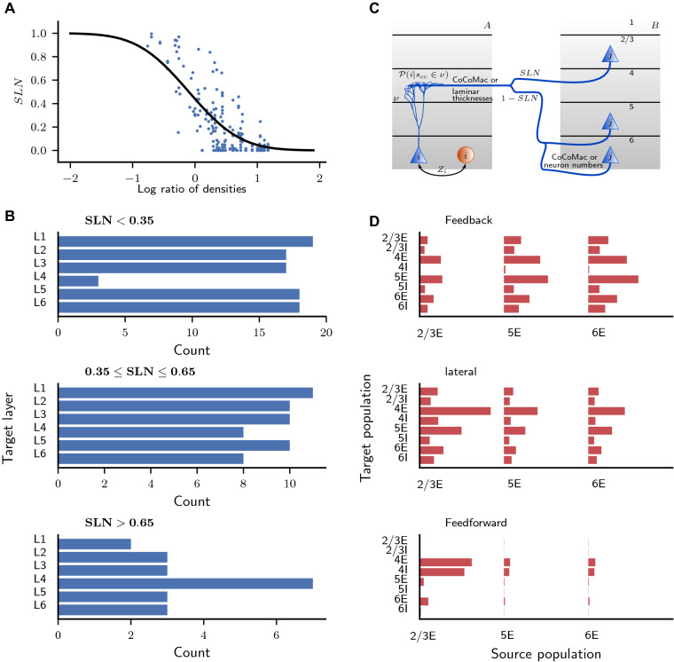
• Figure 5: In panel a, a few data points are missing in the figure. Despite this, the corresponding fit is correct.

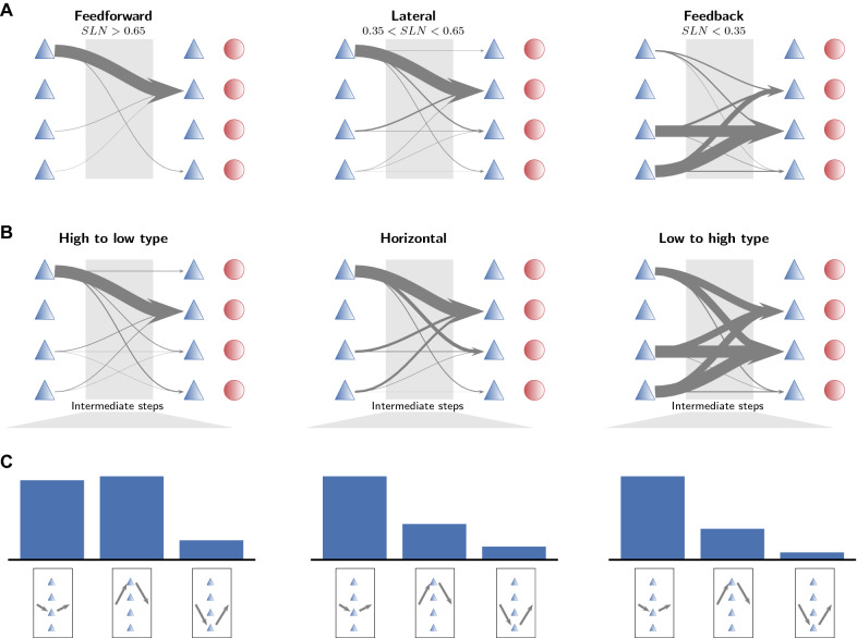
• Figure 8: Due to a mistake in the configuration of parameters, the bottom row of the figure shows wrong results. The published Figure 8c uses $J_{\mathcal{I}}=-11J_{\mathcal{E}}$ instead of the correct value $J_{\mathcal{I}}=-4J_{\mathcal{E}}$. Because of this, the corresponding part of the figure needs to be replaced and the following sentences in the main text are incorrect:

  “In intermediate areas, the shortest paths involve one or two populations. From high-type to low-type areas, these intra-area paths are mostly from 4E to 2/3E (Fig. 8c), in line with the start-end pattern shown in Fig. 8b, but a substantial fraction passes through 2/3E and 5E only. Indirect, horizontal paths mostly involve a relay via 5E, and to a lesser extent 2/3E and the 4E→2/3E pattern. Similarly, connections from late to high-type areas are mostly forwarded by the 5E population only.”

  They should read:

  “In intermediate areas, the shortest paths pass through a single population. From high-type to low-type areas, these paths involve populations 2/3E and 5E about equally. Indirect, horizontal paths mostly involve a relay via 5E, and to a lesser extent 2/3E. Similarly, connections from low-type to high-type areas are mostly forwarded by the 5E population only.”

• Furthermore, we would like to correct two numbers in the main text. In the Results section, we write:

  “CoCoMac provides a binary connectivity matrix with a density of 45% (Fig. 4a). Markov et al. (2014) quantitatively measured connection densities and found a number of previously unknown connections (Fig. 4b) leading to a total of 62% of all pairs of areas being connected.”

  These percentages include some self-connections. The correct numbers without self-connections are 44% and 59% of all disjoint area pairs, respectively. The correct sentence therefore reads:

  “CoCoMac provides a binary connectivity matrix with a density of 44% (Fig. 4a). Markov et al. (2014) quantitatively measured connection densities and found a number of previously unknown connections (Fig. 4b) leading to a total of 59% of all pairs of areas being connected.”

• Finally, the order of the areas in supplementary Fig. S3 was unfortunately incorrect, so that the labels did not match the shown connectivity. We include the figure with the correct ordering of the areas below.

Python code reproducing all results and figures of this work is available from https://inm-6.github.io/multi-area-model/.

Fig. 2.

Aspects of cortical architecture determining population sizes. a Laminar neuron densities for the architectural types in the model. Type 2, here corresponding only to area TH, lacks L4. We treat L1 as containing synapses but no neurons. Data provided by H. Barbas and C. Hilgetag (personal communication). b Total thickness vs. logarithmized overall neuron density and linear least-squares fit ($r=-0.7,p=0.005$). c Relative laminar thickness (see Supplementary Table S3) vs. logarithmized overall neuron density and linear least-squares fits (L1: $r=-0.51,p=0.08$, L2/3: $r=-0.20,p=0.52$, L4: $r=0.89,p=0.0001$; L5: $r=-0.31,p=0.36$, L6: $r=-0.26,p=0.43$). Total cortical thicknesses D(A) and overall neuron densities for 14 areas from Hilgetag et al. (2016) Table 4. The overall densities are based on Nissl staining for 11 areas and for 3 areas on NeuN staining. Laminar neuron densities are based on NeuN staining for all 14 areas. Values based on NeuN staining are linearly scaled to account for a systematic undersampling as determined by repeat measurements in the 11 aforementioned areas

Fig. 5.

Layer- and population-specific cortico-cortical connection patterns. a Fraction of source neurons in supragranular layers (SLN) vs. logarithmized ratio of the overall neuron densities of the two areas. SLN from Markov et al. (2014), neuron densities from Hilgetag et al. (2016). Black curve, fit using a beta-binomial model (Eq. (1); $a_0=-0.152\text{,}{a}_1=-1.534\text{,}\varphi =0.214$). b Laminar target patterns of synapse locations in relation to the SLN value of the source pattern. Target patterns are taken from the CoCoMac database (Felleman and Van Essen 1991; Barnes and Pandya 1992; Suzuki and Amaral 1994; Morel and Bullier 1990; Perkel et al. 1986; Seltzer and Pandya 1994) and SLN data from Markov et al. (2014) mapped to the FV91 scheme. c Illustration of the procedure (Supplementary Eq. 3) for distributing synapses across layers and populations. A source neuron from population j in area B sends an axon to layer v of area A where a cortico-cortical synapse $s_{\mathrm{CC}}$ is formed at the dendrite of a neuron from population i. The dendritic morphology is from Mainen and Sejnowski (1996) (source: NeuroMorpho.org; Ascoli et al. 2007). d Laminar patterns of cortico-cortical connections in the feedback, lateral, and feedforward direction, measured as the indegree of the population pairs divided by the sum of indegrees over all pairs, and then averaged across area pairs with the respective connection type ($K_{\mathit{ij}}={⟨K_{iA,jB}/{\sum }_{i^{\prime },j^{\prime }}{K}_{i^{\prime }A,j^{\prime }B}⟩}_{A,B}$). The categorization into feedback, lateral, and feedforward types follows the SLN value as in B

Fig. 8.

Population specificity organizes paths hierarchically and structurally. a Population-specific patterns of shortest paths between directly connected pairs of areas categorized according to their hierarchical relation as defined by fractions of supragranular labeled neurons (SLN). Arrow thickness indicates the relative occurrence of the particular pattern. The symbols mark excitatory (blue triangles) and inhibitory (red circles) populations stacked from L2/3 (top) to L6 (bottom). b Population-specific patterns of shortest paths between all pairs of areas categorized according to the difference between their architectural types. Arrow thickness indicates the occurrence of the particular pattern. c Occurrence of population patterns in areas that appear in the intermediate stage in the shortest path between two areas

Electronic supplementary material

Below is the link to the electronic supplementary material.

References

- Ascoli GA, Donohue DE, Halavi M. NeuroMorpho.org: a central resource for neuronal morphologies. J Neurosci. 2007;27(35):9247–9251. doi: 10.1523/JNEUROSCI.2055-07.2007. [DOI] [PMC free article] [PubMed] [Google Scholar]
- Barnes CL, Pandya DN. Efferent cortical connections of multimodal cortex of the superior temporal sulcus in the rhesus monkey. J Comp Neurol. 1992;318(2):222–244. doi: 10.1002/cne.903180207. [DOI] [PubMed] [Google Scholar]
- Felleman DJ, Van Essen DC. Distributed hierarchical processing in the primate cerebral cortex. Cereb Cortex. 1991;1:1–47. doi: 10.1093/cercor/1.1.1. [DOI] [PubMed] [Google Scholar]
- Hilgetag CC, Medalla M, Beul SF, Barbas H. The primate connectome in context: principles of connections of the cortical visual system. NeuroImage. 2016;134:685–702. doi: 10.1016/j.neuroimage.2016.04.017. [DOI] [PMC free article] [PubMed] [Google Scholar]
- Mainen ZF, Sejnowski TJ. Influence of dendritic structure on firing pattern in model neocortical neurons. Nature. 1996;382(6589):363–366. doi: 10.1038/382363a0. [DOI] [PubMed] [Google Scholar]
- Markov NT, Vezoli J, Chameau P, Falchier A, Quilodran R, Huissoud C, Lamy C, Misery P, Giroud P, Ullman S, Barone P, Dehay C, Knoblauch K, Kennedy H. Anatomy of hierarchy: feedforward and feedback pathways in macaque visual cortex. J Comp Neurol. 2014;522(1):225–259. doi: 10.1002/cne.23458. [DOI] [PMC free article] [PubMed] [Google Scholar]
- Morel A, Bullier J. Anatomical segregation of two cortical visual pathways in the macaque monkey. Vis Neurosci. 1990;4(06):555–578. doi: 10.1017/S0952523800005769. [DOI] [PubMed] [Google Scholar]
- Perkel DJ, Bullier J, Kennedy H. Topography of the afferent connectivity of area 17 in the macaque monkey: a double-labelling study. J Comp Neurol. 1986;253(3):374–402. doi: 10.1002/cne.902530307. [DOI] [PubMed] [Google Scholar]
- Seltzer B, Pandya DN. Parietal, temporal, and occipita projections to cortex of the superior temporal sulcus in the rhesus monkey: a retrograde tracer study. J Comp Neurol. 1994;343(3):445–463. doi: 10.1002/cne.903430308. [DOI] [PubMed] [Google Scholar]
- Suzuki WL, Amaral DG. Perirhinal and parahippocampal cortices of the macaque monkey: cortical afferents. J Comp Neurol. 1994;350(4):497–533. doi: 10.1002/cne.903500402. [DOI] [PubMed] [Google Scholar]
Associated Data
This section collects any data citations, data availability statements, or supplementary materials included in this article.
Supplementary Materials
Related to Fig. 4. Connection probabilities of the model encoded in color. Areas are ordered according to their architectural types, and populations inside the areas are ordered as [2/3E, 2/3I, 4E/, 4I, 5E, 5I, 6E, 6I] (EPS 3181 kb)