The Invasiveness Classification of Ground-Glass Nodules Using 3D Attention Network and HRCT

Abstract

The early stage lung cancer often appears as ground-glass nodules (GGNs). The diagnosis of GGN as preinvasive lesion (PIL) or invasive adenocarcinoma (IA) is very important for further treatment planning. This paper proposes an automatic GGNs’ invasiveness classification algorithm for the adenocarcinoma. 1431 clinical cases and a total of 1624 GGNs (3–30 mm) were collected from Shanghai Cancer Center for the study. The data is in high-resolution computed tomography (HRCT) format. Firstly, the automatic GGN detector which is composed by a 3D U-Net and a 3D multi-receptive field (multi-RF) network detects the location of GGNs. Then, a deep 3D convolutional neural network (3D-CNN) called Attention-v1 is used to identify the GGNs’ invasiveness. The attention mechanism was introduced to the 3D-CNN. This paper conducted a contract experiment to compare the performance of Attention-v1, ResNet, and random forest algorithm. ResNet is one of the most advanced convolutional neural network structures. The competition performance metrics (CPM) of automatic GGN detector reached 0.896. The accuracy, sensitivity, specificity, and area under curve (AUC) value of Attention-v1 structure are 85.2%, 83.7%, 86.3%, and 92.6%. The algorithm proposed in this paper outperforms ResNet and random forest in sensitivity, accuracy, and AUC value. The deep 3D-CNN’s classification result is better than traditional machine learning method. Attention mechanism improves 3D-CNN’s performance compared with the residual block. The automatic GGN detector with the addition of Attention-v1 can be used to construct the GGN invasiveness classification algorithm to help the patients and doctors in treatment.

Introduction

With the increasing popularization of low-dose CT (LDCT), numerous pulmonary nodules appearing as ground-glass nodules (GGNs) [1] are detected. Although GGNs are slow-growing lesions [2], recent studies have shown that GGNs are closely related to the early stage of lung cancer [3]. The adenocarcinoma appearing as GGN has a development from non-solid to solid. There are similar HRCT manifestations at GGNs’ different development stages. The accuracy of pathological classification is always crucial for the further treatment. Whether the patient is diagnosed with preinvasive lesion (PIL) or invasive adenocarcinoma (IA) has a significant effect on the prognosis and disease-specific survival. Therefore, this paper focuses on the accurate identification of this GGNs’ invasiveness.

The invasiveness categories of lung adenocarcinoma appearing as GGN have become more and more detailed in the latest classification standards. In 2011, the International Association for the Study of Lung Cancer (IASLC), American Thoracic Society (ATS), and European Respiratory Society (ERS) classified small (< 3 cm), solitary adenocarcinomas into four main types: atypical adenomatous hyperplasias (AAH), adenocarcinoma in situ (AIS), minimally invasive adenocarcinoma (MIA), and invasive adenocarcinomas (IA) [4]. The AAH, AIS, and MIA are regarded as preinvasive lesion (PIL). PILs have nearly 100% disease-specific survival, and the IAs’ disease-specific survival is greatly reduced.

Deep learning has been proven to have great advantages over traditional machine learning methods in image classification and target detection [5]. So, the three-dimensional convolutional neural network (3D-CNN) is used to undertake this task. Some study shows that the accuracy of differentiating GGNs’ invasiveness by experienced radiologists is about 80% [6]. Compared with the radiologists, the method proposed by this paper has a better performance.

This paper proposed a new architecture for automatic invasiveness classification. The contributions of this paper are as follows: (1) This paper designed an automatic glass-ground nodule detection algorithm by using a 3D U-Net as the candidate generator and a 3D multi-receptive field network as the false positive reduction method. (2) In order to achieve better performance of predicting the invasiveness probability of GGNs, the attention mechanism is applied to 3D-CNN. (3) This paper combines two modules: the automatic GGN detector and GGN invasiveness classification network, which can automatically detect and analyze the GGN.

Related Work

Recently, deep convolutional neural networks such as faster R-CNN [7] and deep fully convolutional neural network [8] are employed to generate candidate nodules’ bounding boxes. W Zhu et al. [9] used a 3D Faster R-CNN to achieve the candidates. This U-net-like encoder-decoder structure can effectively learn latent features [10]. Then, they designed a special 3D network called dual-path network (DPN). This DPN is mainly used to reduce the false positive rate. Q Dou et al. [11] designed a 3D multi-scale network as the false positive reduction network. They proposed a simple yet effective method to encode multilevel contextual information to meet the challenges coming with the large variations of pulmonary nodules.

Due to the effective performance of U-net-like encoder-decoder, in this paper, a 3D U-Net is designed to obtain candidates’ locations. Meanwhile, a special designed 3D multi-receptive field network (the multi-RF network) is used to conduct the false positive reduction operation. Inspired by the 3D multi-scale network [11], the 3D multi-RF network uses three different receptive field branches to encode the multi-scale features. However, different from multi-scale network, the multi-RF network uses only one input image scale to reduce the input redundancy.

In terms of GGN invasiveness classification, Liu J et al. [12] used multi-detector computed tomography (MDCT) features of PIL and MIA to perform the differentiation diagnosis. This research pointed out that PILs and MIAs have significant differences (P < 0.05) in some features, such as size of lesion, size of solid portion, content of solid portion, and morphological characteristics of the lesion edge. Hwang I et al. [13] used computed tomography texture analysis for differentiating invasive pulmonary adenocarcinomas (IPAs) from preinvasive adenocarcinomas (MIAs) manifesting as persistent pure ground-glass nodules (PGGNs) larger than 5 mm. Each GGN was segmented manually, and their texture features were quantitatively extracted. The multivariate logistic regression and C-statistic analyses were used to identify significant differentiating factors of IPAs from PILs/MIAs. They concluded that CT texture features are significant differentiating factors of IAs presenting as PGGNs larger than 5 mm. These two methods both manually extract the GGN samples and use traditional machine learning method to obtain image features. Recently, the attention mechanism achieves good performance on ImageNet [14]. The SENet [15] introduced the channel attention mechanism to 2D image classification and became the championship of ImageNet2017. The residual attention network [16] applied the spatial attention mechanism to a very deep 2D ResNet [17] and achieved better performance on CIFAR than the original ResNet. Inspired by these two different attention methods, this paper combines the spatial attention mechanism and channel mechanism to construct a dedicated deep 3D attention CNN to automatically classify the invasiveness of the GGNs.

Method

Dataset

Ethical approval was obtained for this retrospective analysis, and informed consent requirement was waived. This paper collected 1431 cases from the cooperative hospital and a total of 1624 GGNs for the experiment. GGNs’ size ranges from 3 to 30 mm. The experimental data were obtained through the labeling of radiologists referenced by pathological reports and HRCTs. The label of dataset consists of three parts: the three-dimensional coordinates of the GGN’s center point in CT image, the invasiveness category, and the diameter.

There are 768 cases that only exist PILs and 663 cases exist IAs. The number of nodules labeled as PILs is 907, and the number of nodules labeled as IAs is 717. The GGNs’ information is shown in Table 1.

Table 1.

The distribution of the GGNs in this study

Diameter (mm)	PIL	IA	Total	P
	907	717	1624
3 < d < 10	470, 51.8%	74, 10.3%	544, 33.5%	< 0.01
10 < d < 20	415, 45.8%	403, 56.2%	818, 50.4%
20 < d < 30	22, 2.4%	240, 33.5%	262, 16.1%

Data Preprocessing

To make the spatial resolution of each HRCT unified and reduce the input redundancy, several methods were used to preprocess the raw 3D-CT image. Firstly, the 3D interpolation was used to reconstruct the HRCT. After reconstruction, the spatial resolution of each HRCT was converted to 1 mm × 1 mm × 1 mm. Finally, the 16-bit signed medical data was converted to 8-bit unsigned integer. The pixel value of each training cubes is bounded from − 1000 to 400 Hu and quantized to an integer from 0 to 255.

Because of the 3D-CNN requires large memory space and computational capacity, this paper selected relatively small 3D data as input. The reconstructed 3D-CT was cropped into a batch of 3D cubes with pixel size 96 × 96 × 96 as the 3D U-Net input. The 3D U-Net was trained by the cropped cubes effectively to conduct pixel-wise classification. This step generated candidates with its center point coordination. Then, the GGN candidates were extracted according to their 3D coordinates with pixel size 48 × 48 × 48 to train 3D multi-RF network.

The train samples of the GGN invasiveness classification network were also extracted by the reconstructed CT images with pixel size 48 × 48 × 48 according to the label. Meanwhile, the train samples were augmented by rotating at arbitrary angles along the X, Y, Z axis with their center point as the origin.

The CNN Architecture

The Automatic GGN Detector: 3D U-Net and Multi-Receptive Field Network

The automatic GGN detector is composed by two steps: GGN candidate detection and false positive reduction.

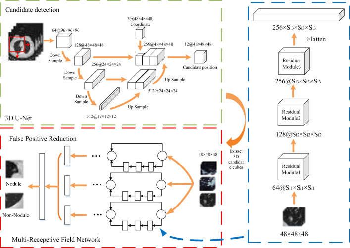
The 3D U-Net is one of the best effective CNN structures to conduct pixel-wise predicting. In order to make the candidate detection more efficient, each CT image is cropped into a batch of image cubes with pixel size of 96 × 96 × 96. The coordinate matrix (the coordinates of input image’s each point in raw CT) is another input of the 3D U-Net to predict the GGN candidates’ center in CT image. The coordinate matrix is scaled with a shape of 48 × 48 × 48 to reduce the memory cost.

Three anchors, 5, 15, 30, are designed for different scale GGNs. According to the label, each GGN is represented by the most appropriate anchor. If an anchor overlaps the GGN ground truth bounding box with the intersection over union (IoU) higher then 0.5, this anchor will be marked as positive (p′ = 1, p′ represents the label of GGN probability). Otherwise, if the IoU less than 0.05, the anchor will be marked as negative (p′ = 0). The GGN ground truth is a sphere segmented from raw CT image whose center point is the GGN’s center and diameter is the GGN’s diameter. Thus, each anchor has two main attributes: GGN probability, center points’ coordinate value of each axis (x, y, z). The multi-task loss function can be defined as

$$L\left(p_{\mathrm{k}},c_{\mathrm{k}}\right)=L_{\text{class}}\left(p_{\mathrm{k}},p{\prime }_{\mathrm{k}}\right)+L_{\text{regression}}\left(c_{\mathrm{k}},c{\prime }_{\mathrm{k}}\right)$$ 1

where p′_k is the ground truth of GGN probability of anchor k, c′_k is the ground truth of GGN’s relative center position of anchor k, p_k and c_k are the prediction of GGN probability and its relative center position. The relative center position c_k and c′_k can be represented as

$$c_{\mathrm{k}}=\left(\frac{x-x_{\mathrm{a}}}{d_{\mathrm{a}}},\frac{y-y_{\mathrm{a}}}{d_{\mathrm{a}}},\frac{z-z_{\mathrm{a}}}{d_{\mathrm{a}}}\right)$$ 2

$$c_{\mathrm{k}}^{\prime }=\left(\frac{x^{\prime }-x_{\mathrm{a}}}{d_{\mathrm{a}}},\frac{y^{\prime }-y_{\mathrm{a}}}{d_{\mathrm{a}}},\frac{z^{\prime }-z_{\mathrm{a}}}{d_{\mathrm{a}}}\right)$$ 3

where (x, y, z) are the regression predict of the anchor center, (x′, y′, z′) are the ground truth position of the anchor center, and (x_a, y_a, z_a, d_a) are the coordinates and anchor size of anchor k. Focal loss function [18] is served as the L_class, and smooth l1 loss function is served as L_regression. The output of the 3D U-Net contains two predictors for each GGN candidate: its center point coordinate and GGN possibility. This information can be used to extract the candidates from the CT image. This method can automatically analyze every anchor in input image. So, we do not need to segment the lung and remove the organs.

After obtaining candidates, the next step is false positive reduction. Due to the fact that diameter of each GGN varies, the network needs to be sensitive to all scale GGNs, especially the small lesions. Different from the multi-scale network, in this paper, the multi-RF network is applied to screen out GGNs. The structure of the multi-RF network is composed of three different branches. Each branch has a specific receptive field [19]. The aim is to increase the sensitivity for GGNs of different sizes with only one input image scale.

As shown in Fig. 1, candidate cubes are trained by three different network branches. Each branch has three residual modules. In order to increase the depth of each branch, this paper chooses ResNet as the basic structure of multi-RF network. Because of the different output shape, flatten operation is conducted before merging features of each branch. In the last layer, the final feature is obtained by merging the three different receptive field branches’ output. Since there are a large number of negative samples during false-positive reduction, focal loss function is served as the classification loss of multi-RF network.

Fig. 1.

The automatic GGN detector’s structure. The resampled CT image is firstly cropped into a batch of image cubes with same shape. Then, the 3D U-Net generates GGN candidates. Finally, false positive reduction is operated by multi-RF network to screen out non-nodule. S_i represents the output shape of the residual module. Due to the different kernel size of each branch, the output shape is different (S_i×S_i×S_i). Flatten operation flats the output of each branch

After finishing training, the model of automatic GGN detector would be used to scan the HRCTs. The GGN location information of each HRCT is obtained and sent to the next classification step.

The GGN Invasiveness Classification Network: the Residual Attention Network

The GGN invasiveness classification network is constructed by assembling multiple cutting edge network structures. The 3D residual block is the basic structure of classification network. Residual blocks are designed to deal with the problem of the gradient vanishing when the network becomes deep.

However, while increasing the capacity of the network, the overfitting risk and the overhead of the network are also increasing. In this task, the original ResNet is modified. The attention mechanism is introduced to construct the classification network.

Attention plays a very important role in human visual cognition [20]. The application of attention mechanism is extensive in computer vision. Several attention structures in computer vision area have been proposed, such as residual attention network [16], SENet [15], and DANet [21]. They are proven to help improve network performance in recent research. However, these attention structures were applied to analyze 2D images. In order to improve the classification performance, this paper modified the basic attention structures to classify 3D medical image.

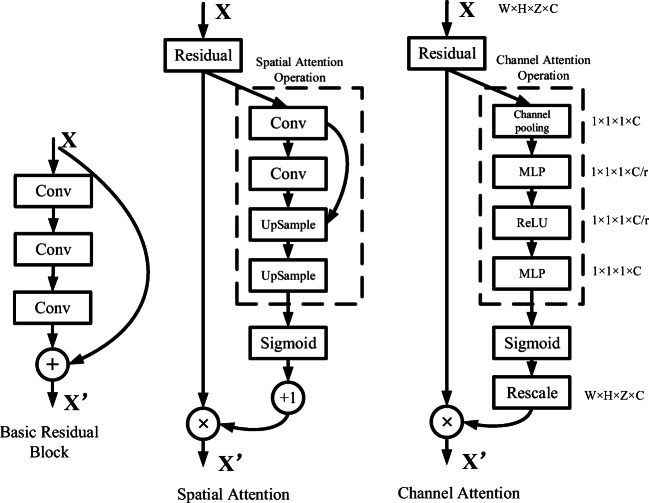
The attention module is composed by spatial attention part and channel attention part. The spatial attention part is a bottom-up top-down feedforward structure [22]. The max pooling operation can be used to down sample the input data. The down-sample and convolution layer are aimed to expand the receptive field and extract the larger-scale feature maps. The feature maps in deeper layer with smaller scales are passed through a convolution transportation layer to restore the shape before down-sampling; it is named as the up-sample operation. The combination of larger scale feature maps and the smaller scale feature maps is used to create the spatial attention part. The detailed structure is shown in Fig. 2.

Fig. 2.

The two parts of the attention module and basic residual block. The spatial attention part: a bottom-up top-down structure, the feature maps in shallow level and deep level are merged to consist the spatial attention feature map. The channel attention part: global pooling to exploit the whole channel filter’s contextual information. The parameter r is equal to 16 in this paper

After conducting the bottom-up and top-down operation, the spatial attention features are extracted from the raw input. Then, Sigmoid function normalizes spatial attention feature to [0–1]. In order to apply the spatial attention feature to the output, the output of the whole part is calculated as

$$F_{\text{spatial}}=\mathrm{\sigma }\left(f_{\text{spatial}}\left(X_{\mathrm{r}}\right)\right)$$ 4

$$O_{\mathrm{s}}=\left(1+F_{\text{spatial}}\right)\odot X_{\mathrm{r}}$$ 5

where σ stands for the activation function sigmoid, f_spatial represents the spatial attention operation, X_r ∈ R^{C × H × W × Z} is the raw input data (the 3D feature maps’ channel size is C, shape is H × W × Z ), F_spatial ∈ R^{C × H × W × Z} is the spatial attention feature which is normalized between 0 and 1, O_s ∈ R^{C × H × W × Z} is the output of the whole part. This is equivalent to

$$O_{\mathrm{s}}=X_{\mathrm{r}}+X_{\mathrm{r}}\odot F_{\text{spatial}}$$ 6

This formula is similar to the operations in the residual block. The spatial attention output can be gradually trained by the back-propagation algorithm. The deep structure of the attention network can extract the 3D image feature from shallow level to deep level. The difference from the traditional residual blocks is the bottom-up top-down structure. This structure is used to extract the spatial attention feature of the original input and limit its range between 0 and 1. This is similar to the gate structure, which will suppress the influence of background on the performance of modules [16]. The parameters of spatial attention part are randomly initialized, and the network will gradually learn its spatial attentional weight by back-propagation.

The channel attention part is constructed by the modified SENet structure; the detail structure is shown in Fig. 2. In order to exploit contextual information of the whole channel filter, the global average pooling operation is used to squeeze the whole channel information into one descriptor. Every channel descriptor has the channel-wise receptive field information. Then, the excitation operator [15] is applied on the channel descriptors. This operation aims to learn the non-linear interaction between descriptors and reduce the network overhead. The excitation operator is composed of two fully connection layers and two activation function. The output of the excitation operation can be calculated by

$$F_{\text{channel}}=f_{\text{Rescale}}\left(\sigma \left(r\left(X_{\mathrm{C}}{W}_{C,\frac{C}{r}}+b_{\frac{C}{r}}\right)W_{\frac{C}{r},C}+b_{\mathrm{C}}\right)\right)$$ 7

The function r represents the activation function ReLU. After passing the global average pooling layer, the input of the channel attention part will become a vector X_c ∈ R^1 × C (C is the channel size of the input data). F_channel ∈ R^{C × H × W × Z} is the output of the excitation operation. Rescale operation f_Rescale rescales vector into the same shape of the input X ∈ R^{C × H × W × Z} by copying the elements of each channel. The full connection weight W_{C, C/r} ∈ R^C × C/r and W_{C/r, C}R^C/r × C are randomly initialized, which make the channel attention vector trained gradually by two multiple perceptions. Finally, the output of the channel attention part O_c ∈ R^{C × H × W × Z} is obtained by

$$O_{\mathrm{c}}=X\odot F_{\text{channel}}$$ 8

where X ∈ R^{C × H × W × Z} stands for the raw input data.

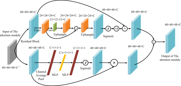
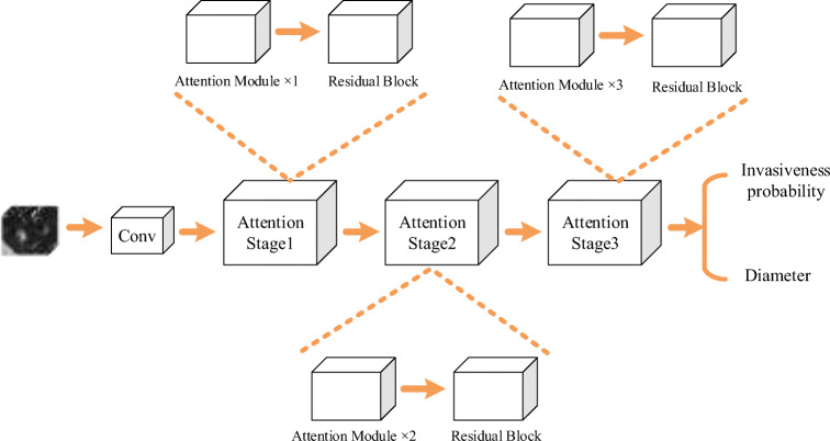
The outputs of the spatial attention part and the channel attention part are merged as the attention module’s output. The spatial attention and the channel attention weights will be gradually trained by back-propagation algorithm. Figure 3 shows the shape changes of the feature map of one attention module. As shown in Fig. 4, the network uses three stages to extract the 3D images’ feature. The attention modules are cascaded after the residual block. This deep 3D residual attention network can also predict the GGN’s diameter accurately. So, this GGN invasiveness classification network’s loss function will be as

$$L\left(p,d\right)=L_{\text{class}}\left(p,p\prime \right)+L_{\text{regression}}\left(d,d\prime \right)$$ 9

Fig. 3.

The data flow in an attention module of stage 1. Cubes colored by the same color represent the same shape of data. C and C′ are the channel sizes

Fig. 4.

The residual attention network structure

where p and d represent the invasiveness probability and diameter (mm) of the network’s output and p′ and d′ denote their ground truth. The binary cross entropy loss function is chosen as the L_class, and the smooth l1 loss function is chosen as L_regression.

The Overall Workflow

The automatic invasiveness classification algorithm is shown in Fig. 5. The overall workflow can be divided into two steps: the detection phase and classification phase.

• ①In training process, the 3D resampled CT image from training samples is served as the input of the automatic GGN detector. The detector will be trained to complete the GGN detection task. Meanwhile, the labeled GGN data is used to train the GGN invasiveness classification model.
• ②In testing process, the test samples in dataset will be in turn put through the GGN detector and invasiveness classification network. The automatic GGN detector will give the predicted GGN’s coordinate in raw CT, and the invasiveness classification network will give the GGN’s invasiveness probability and diameter.

Fig. 5.

The overall workflow of the GGN invasiveness classification algorithm

Experiments and Results

Data Dividing

This paper randomly selected 1158 cases with a total of 1298 GGNs as the training samples. These training cases are used for training the automatic GGN detector and GGN invasiveness network. Five sections for 5-fold cross-validation are divided for training the GGN invasive classification network, so as to make the result more reliable [23–25]. The remaining 273 cases are used as test sets for testing the GGN detector and invasiveness classification network. Data augmentation operations on training GGN samples multiply the number of training sets and increase the robustness of the network.

The Algorithm Performance

Automatic GGN Detector Performance

Firstly, 878 cases of train samples are used to train the 3D U-Net. Then, the rest 280 cases in train samples are scanned by 3D U-Net to test the performance of the model and get the false positive nodules. In the candidate generation phase, the 3D U-Net achieves high sensitivity (98.07%) and relatively low candidate per scan (16.05 candidates per scan). After detecting, 1500 false positive GGNs along with 1298 positive GGNs are used for false positive reduction training. All these candidates are augmented 8 times by 3D rotation for training the false positive reduction network.

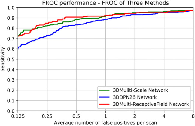
The baseline methods multi-scale network [11] and 3D DPN26 [9] are conducted to evaluate the performance of 3D multi-RF network in the task of false positive reduction. The free-response receiver operating characteristic curves (FROC) and detection performance are shown in Fig. 6 and Table 2. FROC is the average sensitivity at the average number of false positives at 1/8, 1/4, 1/2, 1, 2, 4, 8 per scan, and the competition performance metrics (CPM) is defined as the average sensitivity at these seven false positive rates. The 273 test case samples are used to test the CAD methods. 3D U-Net + multi-RF network has the best performance among three different CAD schemes.

Fig. 6.

The FROC of three nodule detection algorithms

Table 2.

Comparison among different CAD schemes for lung nodule detection

FP/s	1/8	1/4	1/2	1	2	4	8	CPM
3D U-Net + DPN26 [9]	0.603	0.729	0.831	0.885	0.930	0.952	0.968	0.843
3D U-Net + multi-scale [11]	0.733	0.823	0.881	0.918	0.950	0.960	0.970	0.891
3D U-Net + multi-RF	0.712	0.849	0.909	0.922	0.947	0.952	0.976	0.896

Italic entries represent the best results for the performance metrics.

The input size of the multi-RF network and DPN is 48 × 48 × 48. The input size of multi-scale network is 20 × 20 × 6, 30 × 30 × 10, and 40 × 40 × 26. The trainable model parameters of the three networks (multi-RF network, DPN26, and multi-scale network) are 4.6 × 10⁶, 1.8 × 10⁶, and 9.1 × 10⁶. The CPM of 3D U-Net + multi-RF reaches 0.896 better than DPN26 and multi-scale network. This automatic GGN detector can achieve better detection sensitivity at 1/4, 1/2 1, 8 false positive per scan. Moreover, the public database LIDC-IDRI [26] is used to test the generalization ability of the method. Our CAD scheme can also achieve better performance than the other two methods. It is noted that, since most CAD systems used in clinical diagnosis have their internal threshold set to operate somewhere between 1 and 4 false positives per scan on average [27]. The 3D U-Net + multi-RF network fits clinical usage.

In this research, the CAD scheme set 1 false positive GGN per scan among these detected GGNs, and the sensitivity is 0.922. These unavoidable false positive nodules are marked as negative (non-invasiveness) in the next classification step.

GGN Invasiveness Network Performance

The GGN information obtained in the detection network is put into the 3D residual attention network for invasiveness classification. In the experiment, the Attention-v1 network is the classification network proposed by this paper. ResNet-v1 and ResNet-v2 are used as baseline. As shown in Table 3, the Attention-v1 has lower forward FLOPs (floating point operations per second) and less parameter amounts which are 18.11 × 10⁹ and 5.84 × 10⁶. The input size of all these three networks is 48 × 48 × 48. The three networks’ ROC, sensitivity, specificity, accuracy, and AUC are measured and presented in the Fig. 7 and Table 4.

Table 3.

The network structure of the Attention-v1, ResNet-v1, and ResNet-v2

	Attention-v1	ResNet-v1	ResNet-v2
Conv1	5 × 5 × 5, 64	5 × 5 × 5, 64
Attention step 1	Attention module × 1	$\left(\genfrac{}{}{0pt}{}{\mathbf{1}\mathbf{\times }\mathbf{1}\mathbf{\times }\mathbf{1}\mathbf{,}\mathbf{16}}{\begin{array}{c}\mathbf{3}\mathbf{\times }\mathbf{3}\mathbf{\times }\mathbf{3}\mathbf{,}\mathbf{16}\\ \mathbf{1}\mathbf{\times }\mathbf{1}\mathbf{\times }\mathbf{1}\mathbf{,}\mathbf{64}\end{array}}\right)\mathbf{\times }\mathbf{2}$	×3
Residual block 1	$\left(\genfrac{}{}{0pt}{}{\mathbf{1}\mathbf{\times }\mathbf{1}\mathbf{\times }\mathbf{1}\mathbf{,}\mathbf{32}}{\begin{array}{c}\mathbf{3}\mathbf{\times }\mathbf{3}\mathbf{\times }\mathbf{3}\mathbf{,}\mathbf{32}\mathbf{,}\mathbf{\text{stride}}\mathbf{2}\\ \mathbf{1}\mathbf{\times }\mathbf{1}\mathbf{\times }\mathbf{1}\mathbf{,}\mathbf{128}\end{array}}\right)$	$\left(\genfrac{}{}{0pt}{}{\mathbf{1}\mathbf{\times }\mathbf{1}\mathbf{\times }\mathbf{1}\mathbf{,}\mathbf{32}}{\begin{array}{c}\mathbf{3}\mathbf{\times }\mathbf{3}\mathbf{\times }\mathbf{3}\mathbf{,}\mathbf{32}\mathbf{,}\mathbf{\text{stride}}\mathbf{2}\\ \mathbf{1}\mathbf{\times }\mathbf{1}\mathbf{\times }\mathbf{1}\mathbf{,}\mathbf{128}\end{array}}\right)$
Attention step 2	Attention module × 2	$\left(\genfrac{}{}{0pt}{}{\mathbf{1}\mathbf{\times }\mathbf{1}\mathbf{\times }\mathbf{1}\mathbf{,}\mathbf{32}}{\begin{array}{c}\mathbf{3}\mathbf{\times }\mathbf{3}\mathbf{\times }\mathbf{3}\mathbf{,}\mathbf{32}\\ \mathbf{1}\mathbf{\times }\mathbf{1}\mathbf{\times }\mathbf{1}\mathbf{,}\mathbf{128}\end{array}}\right)\mathbf{\times }\mathbf{4}$	×6
Residual block 2	$\left(\genfrac{}{}{0pt}{}{\mathbf{1}\mathbf{\times }\mathbf{1}\mathbf{\times }\mathbf{1}\mathbf{,}\mathbf{64}}{\begin{array}{c}\mathbf{3}\mathbf{\times }\mathbf{3}\mathbf{\times }\mathbf{3}\mathbf{,}\mathbf{64}\mathbf{,}\mathbf{\text{stride}}\mathbf{2}\\ \mathbf{1}\mathbf{\times }\mathbf{1}\mathbf{\times }\mathbf{1}\mathbf{,}\mathbf{256}\end{array}}\right)$	$\left(\genfrac{}{}{0pt}{}{\mathbf{1}\mathbf{\times }\mathbf{1}\mathbf{\times }\mathbf{1}\mathbf{,}\mathbf{64}}{\begin{array}{c}\mathbf{3}\mathbf{\times }\mathbf{3}\mathbf{\times }\mathbf{3}\mathbf{,}\mathbf{64}\mathbf{,}\mathbf{\text{stride}}\mathbf{2}\\ \mathbf{1}\mathbf{\times }\mathbf{1}\mathbf{\times }\mathbf{1}\mathbf{,}\mathbf{256}\end{array}}\right)$
Attention module 3	Attention module × 3	$\left(\genfrac{}{}{0pt}{}{\mathbf{1}\mathbf{\times }\mathbf{1}\mathbf{\times }\mathbf{1}\mathbf{,}\mathbf{64}}{\begin{array}{c}\mathbf{3}\mathbf{\times }\mathbf{3}\mathbf{\times }\mathbf{3}\mathbf{,}\mathbf{64}\\ \mathbf{1}\mathbf{\times }\mathbf{1}\mathbf{\times }\mathbf{1}\mathbf{,}\mathbf{256}\end{array}}\right)\mathbf{\times }\mathbf{6}$	×8
Residual block 3	$\left(\genfrac{}{}{0pt}{}{\mathbf{1}\mathbf{\times }\mathbf{1}\mathbf{\times }\mathbf{1}\mathbf{,}\mathbf{128}}{\begin{array}{c}\mathbf{3}\mathbf{\times }\mathbf{3}\mathbf{\times }\mathbf{3}\mathbf{,}\mathbf{128}\\ \mathbf{1}\mathbf{\times }\mathbf{1}\mathbf{\times }\mathbf{1}\mathbf{,}\mathbf{512}\end{array}}\right)$	$\left(\genfrac{}{}{0pt}{}{\mathbf{1}\mathbf{\times }\mathbf{1}\mathbf{\times }\mathbf{1}\mathbf{,}\mathbf{128}}{\begin{array}{c}\mathbf{3}\mathbf{\times }\mathbf{3}\mathbf{\times }\mathbf{3}\mathbf{,}\mathbf{128}\\ \mathbf{1}\mathbf{\times }\mathbf{1}\mathbf{\times }\mathbf{1}\mathbf{,}\mathbf{512}\end{array}}\right)$
Conv2	1 × 1 × 1, 512	1 × 1 × 1, 512
Average pooling	4 × 4 × 4	4 × 4 × 4
FC, Softmax	13,824
FLOPs × 109	18.11	19.45	24.66
Params × 106	5.84	6.27	6.27

Fig. 7.

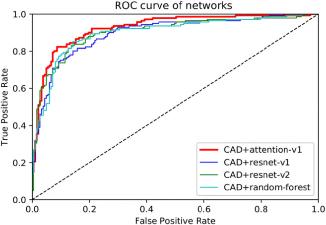
The ROC curve of the four methods. CAD is the above automatic GGN detector

Table 4.

The algorithm performance using four different methods

Network	ACC (0.5 threshold)	Sensitivity	Specificity	AUC
CAD + Attention-v1	85.2%	83.7%	86.3%	92.6%
CAD + ResNet-v1	82.1%	70.9%	90.7%	89.7%
CAD + ResNet-v2	82.7%	71.6%	90.1%	90.3%
CAD + random forest	81.5%	70.2%	91.8%	89.6%

Italic entries represent the best results for the performance metrics

These three networks are configured with exactly the same learning rate, weight decay, and learning rate decay. The difference between Attention-v1 and ResNet-v1 is that the attention module is replaced with residual blocks. In the ResNet-v2 network, the network’s depth was deepened. As the network deepens, the network becomes more complex. This makes the training speed and convergence speed decrease. However, the accuracy and sensitivity of the network have not been significantly improved.

In invasiveness classification task, the AUC value represents the network’s performance. A higher AUC value means better network performance. The AUC value of Attention-v1 is 92.6%, outperforms ResNet-v1 (89.7%), ResNet-v2 (90.3%), and Random-Forest (89.6%). Attention-v1’s sensitivity is also better than ResNet-v1, ResNet-v2, and random forest. However, in terms of specificity, Attention-v1 is about 4% worse than two ResNets and random forest. Some false positives are introduced due to the increased sensitivity, so the Attention-v1’s specificity is reduced. All the three deep learning networks achieve good performance for predicting the GGNs’ diameter, with an average error within 1.5 mm. Two GTX 1080 graphic cards were used to test a series of HRCT samples in parallel, with an average time of 225 s. The time consumption mainly comes from 3D CT reconstruction and window sliding test, which can be further optimized in the future.

Discussion

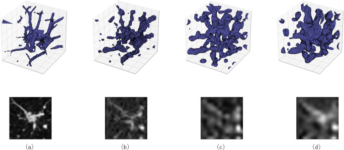
The results are shown in Table 3. Compared with the ResNets, Attention-v1 network has the higher AUC value with less parameters and FLOPs. Attention-v1 also outperforms the traditional machine learning method. The result indicates that deep 3D-CNN can further improve the performance of the classification. The key aspect of deep learning is that these layers of features are not designed by human engineers: they are learned from data using a general purpose learning procedure [28]. The attention mechanism focuses the CNN on the area of interest on the input image. It can also filter the interference caused by the background. After initialization, the weights of spatial attention part and channel attention part optimize automatically by back-propagation algorithm [29]. As shown in Fig. 8, the three attention steps gradually extract image features, from detail to abstraction, from small-scale features to large-scale features.

Fig. 8.

Image generated by intermediate steps in the network. The first row is 3D images generated by marching cubes [30] algorithm (presented with size of 48×48×48). The second row is the same section in 3D images. a Input 3D GGN image. b The output image of attention stage 1. c The output image of attention stage 2. d The output image of attention stage 3

Overfitting is one of the common problems in deep learning. The risk of overfitting increases when the CNN deepens [31]. The ResNets, like ResNet-v1 and ResNet-v2, increase their capacity [32] simply by stacking residual blocks, which has little performance improvement. Meanwhile, the deep 3D ResNets require huge computing resources. The attention mechanism extracts the two different types of the attention information from shallow level to deep level. This attention information can help the CNN achieve better learning performance.

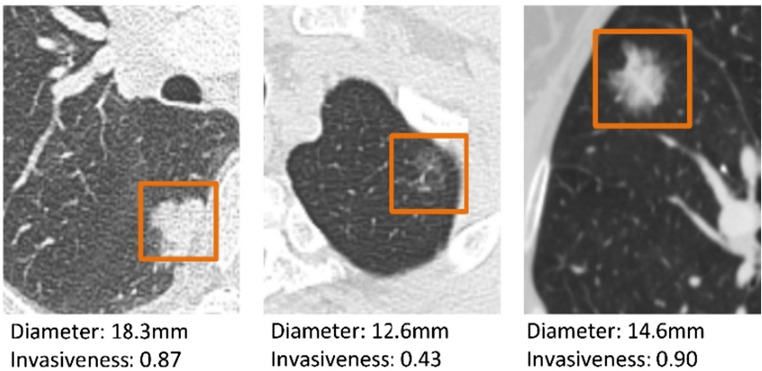
This automatic GGN invasiveness classification algorithm first detects the GGNs’ position in HRCT. Then, the algorithm predicts whether the candidates are PILs or IAs. The GGN detection sensitivity can reach more than 98%, which reduces the burden on radiologists. After completing a case prediction, the algorithm will give us the GGNs’ location, their diameter, and invasiveness probability. This probability can be an important reference for the radiologists. Figure 9 shows the output of the algorithm.

Fig. 9.

The GGN information obtained by the algorithm. Invasiveness means GGNs’ invasive probability

The algorithm is established on the basis of high computing power. Three GTX 1080 GPUs were used for training and one GTX 1080 GPU for testing. 3D networks are expensive to train, so it is important to find leaner networks without sacrificing performance. The attention mechanism is an attempt. Integrative learning of multiple model structures may be one way to improve the performance.

Conclusion

In this paper, a deep 3D-CNN-based algorithm was developed to automatically classify the invasiveness of GGNs. The attention mechanism was introduced into the construction of 3D network and achieved better results compared to the baseline models. This method can provide more rapid and accurate diagnosis reference for radiologists by detecting GGN and displaying the probability of GGNs’ invasiveness. Deep 3D-CNNs showed great potential in distinguishing PILs from IAs; the future work is to build a more efficient and discriminating structure.

Compliance with Ethical Standards

Conflict of Interest

The authors declare that they have no conflict of interest.

Ethical Statement

Ethical approval was obtained for this retrospective analysis, and informed consent requirement was waived.

References

- 1.Qiu ZX, Cheng Y, Liu D, et al. Clinical, pathological, and radiological characteristics of solitary ground-glass opacity lung nodules on high-resolution computed tomography[J] Ther Clin Risk Manag. 2016;12:1445. doi: 10.2147/TCRM.S110363. [DOI] [PMC free article] [PubMed] [Google Scholar]
- 2.Shinohara S, Kuroda K, Shimokawa H, et al. Pleural dissemination of a mixed ground-glass opacity nodule treated as a nontuberculous mycobacterial infection for 6 years without growing remarkably[J] J Thorac Dis. 2015;7(9):E370. doi: 10.3978/j.issn.2072-1439.2015.09.32. [DOI] [PMC free article] [PubMed] [Google Scholar]
- 3.Yamaguchi M, Furuya A, Edagawa M, et al. How should we manage small focal pure ground-glass opacity nodules on high-resolution computed tomography? A single institute experience[J] Surg Oncol. 2015;24(3):258–263. doi: 10.1016/j.suronc.2015.08.004. [DOI] [PubMed] [Google Scholar]
- 4.Travis WD, Brambilla E, Noguchi M, et al. International association for the study of lung cancer/American thoracic society/European respiratory society international multidisciplinary classification of lung adenocarcinoma[J] J Thorac Oncol. 2011;6(2):244–285. doi: 10.1097/JTO.0b013e318206a221. [DOI] [PMC free article] [PubMed] [Google Scholar]
- 5.Hadji I, Wildes R P. What do we understand about convolutional networks?. arXiv preprint arXiv:1803.08834, 2018.
- 6.Wang S, Wang R, Zhang S, et al. 3D convolutional neural network for differentiating pre-invasive lesions from invasive adenocarcinomas appearing as ground-glass nodules with diameters ≤3 cm using HRCT[J] Quant Imaging Med Surg. 2018;8(5):491. doi: 10.21037/qims.2018.06.03. [DOI] [PMC free article] [PubMed] [Google Scholar]
- 7.Ren S, He K, Girshick R, et al. Advances in neural information processing systems. 2015. Faster r-cnn: Towards real-time object detection with region proposal networks[C] pp. 91–99. [DOI] [PubMed] [Google Scholar]
- 8.Long J, Shelhamer E, Darrell T. Proceedings of the IEEE conference on computer vision and pattern recognition. 2015. Fully convolutional networks for semantic segmentation[C]// pp. 3431–3440. [Google Scholar]
- 9.Zhu W, Liu C, Fan W, et al. Deeplung: Deep 3d dual path nets for automated pulmonary nodule detection and classification[C]// 2018 IEEE Winter Conference on Applications of Computer Vision (WACV). IEEE, 2018: 673-681.
- 10.Ronneberger O, Fischer P, Brox T. International Conference on Medical image computing and computer-assisted intervention. Cham: Springer; 2015. U-net: convolutional networks for biomedical image segmentation[C]// pp. 234–241. [Google Scholar]
- 11.Dou Q, Chen H, Yu L, et al. Multi-level contextual 3D CNNs for False positive reduction in pulmonary nodule detection[J] IEEE Trans Biomed Eng. 2016;PP(99):1-1. doi: 10.1109/TBME.2016.2613502. [DOI] [PubMed] [Google Scholar]
- 12.Liu J, Li W, Huang Y, et al. Differential diagnosis of the MDCT features between lung adenocarcinoma preinvasive lesions and minimally invasive adenocarcinoma appearing as ground-glass nodules[J] Zhonghua zhong liu za zhi [Chinese journal of oncology] 2015;37(8):611–616. [PubMed] [Google Scholar]
- 13.Hwang I, Park CM, Park SJ, et al. Persistent pure ground-glass nodules larger than 5 mm: differentiation of invasive pulmonary adenocarcinomas from preinvasive lesions or minimally invasive adenocarcinomas using texture analysis[J] Investig Radiol. 2015;50(11):798–804. doi: 10.1097/RLI.0000000000000186. [DOI] [PubMed] [Google Scholar]
- 14.Deng J, Dong W, Socher R, et al. Imagenet: A large-scale hierarchical image database[C]// 2009 IEEE conference on computer vision and pattern recognition. Ieee, 2009: 248-255.
- 15.Hu J, Shen L, Sun G. Proceedings of the IEEE conference on computer vision and pattern recognition. 2018. Squeeze-and-excitation networks[C]// pp. 7132–7141. [Google Scholar]
- 16.Wang F, Jiang M, Qian C, et al. Proceedings of the IEEE Conference on Computer Vision and Pattern Recognition. 2017. Residual attention network for image classification[C]// pp. 3156–3164. [Google Scholar]
- 17.He K, Zhang X, Ren S, et al. Proceedings of the IEEE conference on computer vision and pattern recognition. 2016. Deep residual learning for image recognition[C]// pp. 770–778. [Google Scholar]
- 18.Lin TY, Goyal P, Girshick R, et al. Focal loss for dense object detection[J] IEEE Trans Pattern Anal Mach Intell. 2017;PP(99):2999–3007. doi: 10.1109/TPAMI.2018.2858826. [DOI] [PubMed] [Google Scholar]
- 19.Gilbert CD, Wiesel TN. Receptive field dynamics in adult primary visual cortex[J] Nature. 1992;356(6365):150–152. doi: 10.1038/356150a0. [DOI] [PubMed] [Google Scholar]
- 20.Itti L, Koch C. Computational modelling of visual attention[J] Nat Rev Neurosci. 2001;2(3):194–203. doi: 10.1038/35058500. [DOI] [PubMed] [Google Scholar]
- 21.Fu J, Liu J, Tian H, et al. Proceedings of the IEEE Conference on Computer Vision and Pattern Recognition. 2019. Dual attention network for scene segmentation[C]// pp. 3146–3154. [Google Scholar]
- 22.Anderson P, He X, Buehler C, et al. Proceedings of the IEEE conference on computer vision and pattern recognition. 2018. Bottom-up and top-down attention for image captioning and visual question answering[C]// pp. 6077–6086. [Google Scholar]
- 23.Chang J S, Luo Y F, Su K Y. GPSM: a generaized probabilistic semantic model for ambiguity resolution[C]// Proceedings of the 30th annual meeting on Association for Computational Linguistics. Association for Computational Linguistics, 1992: 177-184.
- 24.Kohavi R. A study of cross-validation and bootstrap for accuracy estimation and model selection[C]// Ijcai. 1995;14(2):1137–1145. [Google Scholar]
- 25.Ling CX, Huang J, Zhang H. Conference of the Canadian society for computational studies of intelligence. Berlin: Springer; 2003. AUC: a better measure than accuracy in comparing learning algorithms[C]// pp. 329–341. [Google Scholar]
- 26.Armato SG, Mclennan G, Bidaut L, et al. The lung image database consortium (LIDC) and image database resource initiative (IDRI): a completed reference database of lung nodules on CT scans [J] Med Phys. 2011;38(2):915–931. doi: 10.1118/1.3528204. [DOI] [PMC free article] [PubMed] [Google Scholar]
- 27.Ding J, Li A, Hu Z, et al. Accurate pulmonary nodule detection in computed tomography images using deep convolutional neural networks[J] 2017. [Google Scholar]
- 28.LeCun Y, Bengio Y, Hinton G. Deep learning[J] Nature. 2015;521(7553):436–444. doi: 10.1038/nature14539. [DOI] [PubMed] [Google Scholar]
- 29.Rumelhart DE, Hinton GE, Williams RJ. Learning representations by back-propagating errors[J] Nature. 1986;323(6088):533–536. doi: 10.1038/323533a0. [DOI] [Google Scholar]
- 30.Lorensen WE, Cline HE. Marching cubes: A high resolution 3D surface construction algorithm[J] ACM Siggraph Comput Graph. 1987;21(4):163–169. doi: 10.1145/37402.37422. [DOI] [Google Scholar]
- 31.Tetko IV, Livingstone DJ, Luik AI. Neural network studies. 1. Comparison of overfitting and overtraining[J] J Chem Inf Comput Sci. 1995;35(5):826–833. doi: 10.1021/ci00027a006. [DOI] [Google Scholar]
- 32.Keskar N S, Mudigere D, Nocedal J, et al. On large-batch training for deep learning: generalization gap and sharp minima. In The International Conference on Learning Representations (ICLR), 2017.