

Abstract
Dengue is a vector-borne disease transmitted by the Aedes genus mosquito. It causes financial burdens on public health systems and considerable morbidity and mortality. Tropical regions in the Americas and Asia are the areas most affected by the virus. Fortaleza is a city with approximately 2.6 million inhabitants in northeastern Brazil that, during the recent decades, has been suffering from endemic dengue transmission, interspersed with larger epidemics. The objective of this paper is to study the impact of human mobility in urban areas on the spread of the dengue virus, and to test whether human mobility data can be used to improve predictions of dengue virus transmission at the neighbourhood level. We present two distinct forecasting systems for dengue transmission in Fortaleza: the first using artificial neural network methods and the second developed using a mechanistic model of disease transmission. We then present enhanced versions of the two forecasting systems that incorporate bus transportation data cataloguing movement among 119 neighbourhoods in Fortaleza. Each forecasting system was used to perform retrospective forecasts for historical dengue outbreaks from 2007 to 2015. Results show that both artificial neural networks and mechanistic models can accurately forecast dengue cases, and that the inclusion of human mobility data substantially improves the performance of both forecasting systems. While the mechanistic models perform better in capturing seasons with large-scale outbreaks, the neural networks more accurately forecast outbreak peak timing, peak intensity and annual dengue time series. These results have two practical implications: they support the creation of public policies from the use of the models created here to combat the disease and help to understand the impact of urban mobility on the epidemic in large cities.
Keywords: dengue, forecasting, neural network, human mobility
1. Introduction
Dengue (DENV) is an arbovirus transmitted by the Aedes genus mosquito with four serotypes (DENV-1, DENV-2, DENV-3 and DENV-4) and is present all over the world. It is estimated there are 390 million dengue cases per year [1] with 40% of the world population living in an area of risk [2]. Tropical regions are most affected by the virus, and the highest risk of transmission occurs in the Americas and Asia. DENV causes various symptoms including fever, headache, nausea and vomiting, and in its most severe form, dengue haemorrhagic fever, may lead to death [3].
Fortaleza is the fifth most populous city in Brazil with a population of approximately 2 600 000 inhabitants [4] and an area of 314 930 km2. In 1994, the serotype DENV-2 was introduced into Fortaleza and caused a large epidemic of dengue. Since then several additional dengue epidemics have occurred in the city [5,6]. In Brazil, the dominant vector of dengue is Aedes aegypti. In areas with high levels of dengue transmission, public officials visit households during the mosquito breeding season to search for mosquito larvae and to apply larvicide; however, these vector control methods have had limited success [7–10].
As a means of helping combat dengue virus transmission, a number of forecasting systems have been proposed with the aim of predicting dengue epidemics in urban areas at different geographic levels [11–17]. One class of disease forecasting method uses machine learning models. In [18], the authors proposed an XGBoost model to classify dengue outbreaks using five climate variables—temperature, rainfall, humidity, air pressure and wind speed. In [19], a support vector machine model was trained to forecast morbidity rates in three provinces in Thailand based on dengue cases, weather and mosquito data. The research in [20] proposed a three-layer neural network model to forecast dengue outbreaks at the district level based on dengue history and rainfall data. The authors compared the neural network with a nonlinear regression model and found that the neural network model resulted in a much smaller mean square error (MSE). A second class of disease forecasting system uses mechanistic models coupled with data assimilation methods [21–23]. These systems represent disease transmission mathematically as an initial value problem and optimize simulation and forecast using observations and data assimilation. Several of these systems have been deployed to predict dengue [24,25].
Although the movement capabilities of Aedes aegypti in urban areas are small, around 25 m [26], the transmission of dengue virus across long distances occurs with the movement of infected humans. As a consequence, the impact of human mobility on dengue transmission has been studied on a number of scales: residential [27–30], city block [31], district [32,33], municipal [34–36] and state [37]. Displacement patterns can support the prediction of the next site where the epidemic will spread, which can be useful in planning mosquito control efforts. Thus, anticipating which sites are more likely to have a large-scale epidemic results in more efficient prevention policies.
The use of human mobility data to improve the accuracy of predicting dengue incidence is recent. An example is [38], which used LASSO regression [39] with the objective of classifying neighbourhoods at high or low risk with respect to the incidence of dengue in Singapore. Human mobility was analysed through activity data obtained from a mobile phone network and incorporated into the model to predict dengue cases up to 12 weeks ahead. In another study using mobile data, mechanistic models were developed to predict dengue cases [40].
For this study, our primary objective is to evaluate three different types of forecast models and compare their capacity to capture the nonlinear relationships between human mobility and disease characteristics and to make accurate early epidemic predictions. We developed two dengue forecasting systems using distinct methods: a multi-layered neural network architecture and a mechanistic disease transmission model coupled with the ensemble adjustment Kalman filter (EAKF). We also used an autoregressive integrated moving average (ARIMA) model as baseline. These systems use historical time series of dengue incidence as input. We then quantified the effect of human mobility data on each forecasting system by producing forecasts with and without public transportation passenger mobility data. These systems use a space–time graph describing the movement of people within Fortaleza in addition to historical dengue incidence data.
Forecasts were evaluated for their ability to differentiate periods with and without large-scale epidemics, for detecting peak intensity as well as the date of peak incidence, and for predicting the dengue incidence time series for the entire year. In general, both the neural network approach and mechanistic models obtained improved results when using the mobility data, providing evidence that movement patterns have the potential to indicate the emergence of epidemics. In particular, with the use of mobility information, the neural network was able to predict the intensity and timing of dengue peak incidence and timing further in advance, which can be important and helpful for planning the fight against the spread of dengue.
2. Material and methods
2.1. Data
In order to develop a predictive model of dengue and to study the impact of human mobility on dengue virus transmission, two datasets from the city of Fortaleza were used: a dataset of dengue confirmed cases and a dataset describing human mobility by public transportation (datasets and codes available at https://github.com/rafaellpontes/denguėmobilitẏpaper).
Since 2007, the Municipal Health Department of Fortaleza has monitored dengue incidence through the reporting of dengue cases diagnosed in hospitals or primary health care units in the public health network. The records are stored with the patient’s home address and the date of diagnosis, allowing for the aggregation and identification of weekly cases for the 119 neighbourhoods of the city. The data are available on the Sistema de Monitoramento Diário de Agravos—SIMDA (Daily Disease Occurrence Monitoring System) [41]. From SIMDA we extracted data from 2007 to 2015: a total of 174 954 dengue cases, as shown in figure 1.
Figure 1.

Time series of dengue cases in Fortaleza from 2007 to 2015.
In order to capture human movement in the city of Fortaleza, bus transportation data from the public transportation system for the year 2015 were used. In Fortaleza, the bus system is the most widely used mode of transport encompassing, in 2015, 356 bus lines, 2034 buses and 700 000 users, totaling an average of 1 million trips per day [42]. In this study, the mobility of people in the city was represented by data produced in [43] giving the origin and destination bus stops of users of the city bus system. The origin is recorded from the electronic bus pass used by the user at the time of boarding the bus. The destination point is estimated by the second boarding made by the same user on the same day. For example, for a user who boarded a bus at stop BS1 in the morning and at the end of the day entered a bus at stop BS2, it is assumed that there was a trip from the origin BS1 to the destination BS2. If a user has boarded three buses in a day using the stops BS1, BS2 and BS3, two trips are generated for this user, the first trip starting at BS1 and finishing at BS2 and the second trip starting from BS2 and finishing at BS3. Further details of the methodology can be seen in [43]. Overall, the authors show, by exploring the journeys made by about 500 000 people a year and traversing 4783 geo-referenced bus stops, that the data are not spatially biased and significantly represent the movement of the city’s population. Some studies have used these data in recent years for various purposes such as understanding crime and identifying traffic bottlenecks [44–48]. Here, we used the coordinates of each bus stop to spatially aggregate bus data to the neighbourhood level. The daily bus data were averaged over the course of a week. The resulting dataset of weekly flow rates between each of the 119 neighbourhoods served as the input for the geographically linked forecast systems. Human mobility between neighbourhoods was modelled as a graph (figure 2) where the nodes are the neighbourhoods and the weights of the edges are a flow rate (equation (2.1)) representing the flow of people (flowratei,k,w) from neighbourhood i to neighbourhood k in week w, computed as:
| 2.1 |
count (flowi,k,w) is the number of bus journeys from neighbourhood i to neighbourhood k in week w. TN is the total number of neighbourhoods in the city.
Figure 2.

The weekly flow of people across neighbourhoods. The yellow arrows drawn on the map highlight an example of flow between seven neighbourhoods. flowrate4,5,1 represents the flow from neighbourhood 4 to neighbourhood 5 in week 1. The full model includes flow rates to and from each of the city’s 119 neighbourhoods for every week of the entire period.
2.2. Neural network models
We propose two recurrent neural network (RNN) [49] architectures to determine the impact of public transportation on forecasting the spread of the dengue virus: one, RNNi, which considers dengue cases in each neighbourhood in isolation, and a second, RNNc, which uses the bus transportation data to link neighbourhoods. RNNs are a type of architecture that learn the temporal dependence of a variable through the recurrent application of backpropagation through time (BTT). Figure 3 illustrates the basic idea behind this concept.
Figure 3.

Recurrent neural network temporal prediction flow. U, V and W are the network parameters. X and Y are model input and prediction, respectively. S is the model state and t is time.
The principle of this technique is that it is possible to calculate the error gradient with respect to the network parameters (e.g. U, V and W in figure 3) and then learn improved parameters using stochastic gradient descent. Just as we sum up the errors, we also sum up the gradients at each time step for one training. To calculate these gradients, we use the chain rule of differentiation which is the backpropagation algorithm when applied backwards starting from the error.
Figure 3 shows prediction flow performed by the RNN where each state S is impacted by the input X (in this instance, cases of dengue) and by the previous state to achieve the prediction at a specific time. Specifically, in time-series learning the use of backpropagation in RNNs makes it impossible to learn very long time dependencies due to the vanishing gradient problem. This problem occurs when an RNN works with large recurrences, such that during the process of backpropagation the gradient becomes very small and the weights of the RNN do not change.
Long short-term memory (LSTM) [50] is a type of RNN that mitigates the vanishing gradient problem. LSTM solves this problem with an architecture that incorporates a cell memory and a set of gates (input, output and forget gates) that regulate the input and output of cell memory information. Figure 4 and the following equations explain the LSTM unit S.
| 2.2 |
| 2.3 |
| 2.4 |
| 2.5 |
| 2.6 |
| 2.7 |
where the Wix, Wic, Wfc and Woc are the weight matrices, b are the vectors of bias (bi, bf, bc, bo and by), σ, the logistic sigmoid function and i, f, o and c are respectively the input gate, forget gate, output gate and cell activation vector. m the output vector, is the element-wise product of vectors, and g and h are the cell input and cell output activation functions.
Figure 4.
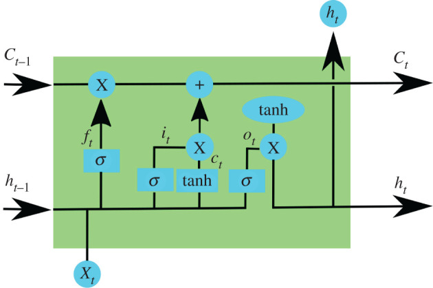
An LSTM unit has a chain structure that contains four neural networks and different blocks of memory called cells. The information is retained by the cells and the memory manipulations are made through the input (it), forget (fi) and output (oi) gates. Long-term memory is usually called the cell states on which information from previous intervals are stored.
We first proposed an isolated architecture, RNNi, that predicts dengue cases for a specific neighbourhood based only on its own past dengue case data using LSTM. This model was developed for each of the 119 neighbourhoods of Fortaleza using two inputs: a time series with the weekly number of dengue cases for a neighbourhood (the entry window is five weeks) and an index vector, ranging from 1 to 52, that labels each of these five weeks. This vector feeds an embedding layer that generates an output to be concatenated with dengue cases. The concatenated data feed an LSTM that connects to an output layer (dense layer) with a sigmoid activation function and generates the prediction of the dengue cases for the following week.
Dropout layers were introduced for avoiding overfitting. Dropouts layers randomly force a given percentage of the previous layer’s neurons to be ignored during each training step in order to avoid overfitting by a single path of neurons. Figure 5 illustrates the architecture for the RNNi model with its input and output data and layers. The dropout layers enable the measurement of the variability of the forecasts. In order to generate a probabilistic forecast, we used Monte Carlo dropout (MC dropout) [51] to generate n = 100 realizations of predictions by randomly assigning the probabilities of the dropouts (dropout rate) existing after each layer.
Figure 5.

Neural network isolated architecture—the RNNi model. The isolated architecture predicts one week ahead of dengue cases for a specific neighbourhood based on the past five weeks of dengue cases and an index vector labelling each entry week. The embedding layer learns a representation for each week’s label, which is concatenated with the dengue data. Thus, the evolution of the dengue cases is learnt through the concatenated data, then the dense layer outputs the prediction for the week ahead. The values in parentheses in the dropout represent the fraction of neurons to ignore in each training step. The values between brackets represent the data dimensions of input and output for each layer.
The RNNi model should be capable of anticipating several weeks ahead in order to provide actionable forecasts. There are several strategies to address the problem of multi-step prediction, such as (recursivity, direct, direct-recursivity and multi-output strategy) [52,53]. Here, we used the recursive strategy. This strategy performs the first prediction based on observed incidences, but uses the predicted values recursively to predict the rest of the time series.
The second architecture, RNNc, predicts dengue cases for all neighbourhoods simultaneously using historical data of dengue as in the isolated architecture, and human mobility (represented as described in figure 2). A representation of each node was generated using node embedding techniques and, together with the past dengue data, used as input data for a hierarchical LSTM architecture.
The RNNc architecture uses a hierarchical structure, with the RNNi model representing the lower level. This architecture captures human mobility and its impact on dengue virus transmission.
The node embedding algorithm, Node2Vec [54,55], was used to learn the characteristics of each node of the human mobility graph. Node2Vec uses a neural network to capture the context around the node. This is done by generating embeddings, which are one-dimension-vectorial representations of the graph nodes. In our case, each vector produced by Node2Vec is a sequence of neighbourhoods of a predetermined length. This sequence is produced by a weighted random walk to an adjacent node. The basic idea behind random walk based embedding techniques is to transform the graph into a collection of node sequences in which the occurrence frequency of a node-context pair measures the structural distance between them.
Several values for the size of the embedding have been tested; size 15 was defined for the embedding of each neighbourhood. It was used as an input for the model together with the weekly dengue cases of all the neighbourhoods as well as the embedding representing the week (using the index vector previously described for the baseline). These three components feed three LSTM layers that aim to capture the spatio-temporal relation of the dengue cases. Thus, the RNNc model (figure 6) predicts the weekly dengue cases for all the neighbourhoods simultaneously based on the incidence of neighbourhood-level dengue data for the entire city and on human mobility data.
Figure 6.

Artificial neural network architecture for the RNNc networked model using human mobility data. The architecture assumes the input of three datasets: the five-week temporal series from 119 neighbourhoods, a vector with one id for each week and a vector representation (embbedings) describing the transport information for each neighbourhood. The values inside the brackets represent the dimension of each dataset. The dimension of the inputs are: [5, 119] representing the dimension of the matrix containing five week of dengue cases for all the 119 neighbourhood; [5, 1] representing a vector with the indices for each week and [5, 1785] representing five weeks and the embedding of size 15 representing the flow among the 119 neighbourhoods (15 × 119 = 1785). The dimension of the hidden layer concatenate is [5, 271] representing the concatenation of the columns of the three input layers. A stack of LSTMs (the figure shows the unfolded LSTMs) is fed with the concatenation results and each layer of the stack propagates information (dimension 300) for the next layer. The last layer of the stack is fully connected with a dense layer (output layer) to predict the dengue case of each one of the 119 neighbourhoods.
Cross-validation was applied to all 9 years of data available, from 2007 to 2015. For each year to be predicted, 2 years were used to evaluate the model (one epidemic year and the other without an epidemic) and the rest of the data was used to train the model. Table 1 shows for each test year the breakdown of the years used to define the validation and training basis.
Table 1.
Data division for cross-validation. Validation data are used to adjust the model parameters during the training phase, while the test data are used to evaluate the final performance of the model.
| test | evaluation | training |
|---|---|---|
| 2007 | 2010, 2012 | 2008, 2011, 2012, 2013, 2014, 2015 |
| 2008 | 2010, 2012 | 2007, 2011, 2012, 2013, 2014, 2015 |
| 2009 | 2010, 2012 | 2007, 2008, 2011, 2012, 2013, 2014, 2015 |
| 2010 | 2007, 2012 | 2008, 2011, 2012, 2013, 2014, 2015 |
| 2011 | 2010, 2012 | 2007, 2008, 2012, 2013, 2014, 2015 |
| 2012 | 2007, 2015 | 2007, 2008, 2011, 2013, 2014, 2015 |
| 2013 | 2010, 2012 | 2007, 2008, 2011, 2012, 2014, 2015 |
| 2014 | 2010, 2012 | 2007, 2008, 2011, 2012, 2013, 2015 |
| 2015 | 2010, 2012 | 2007, 2008, 2011, 2012, 2013, 2014 |
2.3. Mechanistic models
In order to further assess the impact of human mobility on dengue forecasting, we performed a second set of comparisons. We generated forecasts using a system developed with a mechanistic model, with and without the inclusion of human mobility data. Due to the interpretability of mechanistic models, process-based forecasting systems have been widely used in predicting infectious disease outbreaks [56–60], including dengue [25], Ebola [61], influenza-like illness [62] and antibiotic-resistant pathogens [63].
The local forecasting system, MECHi, makes use of incidence data from each neighbourhood, and predicts the epidemic curves independently for different locations. Due to a lack of detailed mosquito data, we model the transmission of dengue virus in each neighbourhood using a parsimonious susceptible–exposed–infected–recovered (SEIR) model:
| 2.8 |
| 2.9 |
| 2.10 |
where N, S, E and I are the number of total, susceptible, exposed and infectious people, respectively; β is the transmission rate; Z is the latency time; and D is the infectious period. For the networked forecasting system, MECHc, we connect neighbourhoods by considering the mixing of the population due to bus transportation. The transmission across 119 neighbourhoods is described by a networked SEIR model [61]:
| 2.11 |
| 2.12 |
| 2.13 |
Here Si, Ei and Ii are the number of susceptible, exposed and infectious people in neighbourhood i; βi is the transmission rate in location j; cji is the fraction of the population travelling from neighbourhood i to j; and is the total population present in location j. The human mobility information cji is obtained from the bus transportation data. In both models, the initial ranges of variables and parameters are set as follows: S ∈ [0.3, 0.55]N, E ∈ [0, 0.0005]N, I ∈ [0, 0.0005]N, β ∈ [0.3, 0.5], days, days, and N is set as the population in each neighbourhood.
To estimate model variables and parameters using observed incidence, we use a data assimilation algorithm—the EAKF [64]. Specifically, model state variables and parameters are iteratively adjusted using observations from the season onset to the present, and the optimized model is integrated into the future to generate forecasts. With the EAKF, the distribution of the model state is represented by an ensemble of state vectors. As a result, the forecast system is able to generate probabilistic predictions. For our implementation, we used 300 ensemble members. Similar model-data assimilation frameworks have been successfully applied to the forecast and inference of influenza [56–60], dengue [25], Ebola [61], influenza-like illness [62] and antibiotic-resistant pathogens [63]. In particular, a similar networked forecasting system has been recently used to predict the spatial transmission of influenza in the USA [65]. In the electronic supplementary material, there are forecast examples for the mechanistic and neural network models.
2.4. Evaluation of retrospective forecast
To examine how many weeks in advance the models can predict peaks of dengue cases, predictions were generated starting from week 6 to week 25 of the year, which we consider to be the dengue season. For each forecasting week, predictions were generated for the remainder of the year for each neighbourhood, with three objectives: to classify years and neighbourhoods with and without intense outbreaks, to predict the peak intensity and peak timing, and to predict the entire time series of dengue cases for intense outbreaks. Neighbourhoods with greater than 200 dengue cases in a year were classified as intense. In addition, we tested the sensitivity to this threshold value. To measure the classification of outbreaks as intense or not, we have used precision and recall metrics as follows:
| 2.14 |
and
| 2.15 |
where (TP) is true positive, (TN) is true negative, (FP) is false positive and (FN) is false negative.
In order to evaluate the forecasts of peak intensity (PI) and peak timing (PT), we calculated the mean absolute error (MAE) as the difference between the actual and predicted PI and PT, respectively:
| 2.16 |
and
| 2.17 |
where, for PI, y is the real number of dengue cases during the peak week and is the predicted number of dengue cases during the peak week. For PT, r is the index of the peak week of the real time series, the index of the peak week of the predicted time series, and K is the total number of outbreaks with annual cases of infections higher than 200. To measure the error of the time series prediction, root mean square error (RMSE) was calculated between the real and predicted time series of dengue cases for each large outbreak. In general, the time series of dengue cases in Fortaleza show few peaks in the year. So the most important thing for a forecasting model is to identify the peak and its ups and downs. RMSE (see equation (2.18)) is the most appropriate metric to capture this because the difference between the predicted value for the real is raised to the power of two before the average is retained. This causes great differences to be highlighted as bad forecasts during critical periods when incidence is high are penalized.
| 2.18 |
x is the total number of dengue cases in the real outbreak, is the total number of dengue cases in the predicted outbreak, W is the total number of weeks in the year and f is the forecasting time, the week of the year that the forecasting was initiated. RMSE is measured for each large outbreak and finally the average of all outbreaks is calculated.
As a final comparison, the results of the RNNi and MECHi models were compared with an ARIMA [66]. ARIMA is a widely studied statistical univariate model for time-series prediction and used in various domains. [67–69].
Through auto-correlation analysis (detailed in the auto-correlation electronic supplementary material), we see that the number of dengue cases has high correlation with previous values, that is, with small lags. Thus, ARIMA was performed for auto-correlation value 5 (AR (5)) and moving average value 1 (MA (1)).
We evaluated the probabilistic forecasts by computing their log score, a commonly used forecast scoring method [24,70,71]. For peak intensity, the log score of the prediction for an intense outbreak is the logarithmic value of the percentage of predictions that falls within an interval of ±10 cases around the actual case number. For peak timing, the log score is the logarithmic value of the percentage of predictions that falls within an interval of ±1 week of the actual peak week, and for time-series prediction, the average of logarithmic values of the percentage of predictions of weekly dengue cases for the remaining weeks of the dengue season that fall within ±10 cases of the observed cases. Each measurement was averaged over the weekly forecasts for all intense outbreaks in all neighbourhoods. By definition, a higher log score indicates a better forecast performance. When the average percentage of previsions is zero, the constant −5 is assumed by default as a penalizing value.
3. Results
As a baseline, we compared the isolated mechanistic and RNN forecasts with a standard ARIMA forecast, ARIMAi for local forecast and ARIMAc (using ARIMAX) for forecasting considering all the neighbourhoods. Figure 7 shows the results of precision and recall for years and neighbourhoods with and without intense epidemics obtained from all the models. Precision and recall are evaluation metrics for classification problems. In this case, precision measures the fraction of correct classification of intense epidemics, , from all the cases predicted as intense epidemics, and the recall measures the correct classified intense epidemics from all intense epidemics that actually happened. The same holds for non-epidemic classifications, .
Figure 7.

For all plots, axis x indicates the week in which the forecast is generated. Axis y shows the values for precision, recall and F-score. For example, in (a), the value of y for x = 12 (forecasting time = 12) shows the precision calculated from predictions made starting at week 12 until the last week of the year (week 52). (a) The precision of the classification for seasons with total dengue cases less than or equal to 200, (b) the recall of the classification for seasons with total dengue cases less than or equal to 200, (c) F-score of the classification for seasons with dengue cases greater than 200, (d) the precision of the classification for seasons with total dengue cases greater than 200, (e) the recall of the classification for seasons with total dengue cases greater than 200 and (f) F-score of the classification for seasons with total dengue cases less than or equal to 200.
With the dengue epidemics classification problem, both models obtained better performance when considering transportation data (RNNc and MECHc). Although the MECHc had less precision than the RNNc model, the mechanistic model exhibited a higher recall in prediction times closer to the beginning of the year, indicating that the MECHc model better forecasts large outbreaks (high recall for dengue cases >200). This implies that the networked MECHc model tends to predict large outbreaks, but will overestimate some small outbreaks. In general, both the RNNc and MECHc can classify the dengue outbreak size with a satisfactory performance. As for the model generated by ARIMAi, there is a high recall for small outbreaks (figure 7b). This is because, in these cases, there are no requirements for the model to capture important variations and thus the model ends up performing well in periods when there was no peak in dengue cases. However, when we analyse the recall of this model in cases with large peaks (figure 7e), the results are not good. The behaviour is particularly poor for the early forecast time. The same behaviour is observed when analysing the precision values. Since most of the predictions made by ARIMAi were defined as periods without peak dengue cases, then the precision values are expected to be low for periods with dengue cases ≤200 and for periods with dengue cases >200 the high values given that few periods were predicted as large outbreaks. The results for the ARIMAc model are even worse than the results of ARIMAi, indicating that when the complexity of the problem is increased, models of the ARIMA type fail to present reasonable results. The analysis regarding precision and recall can be summarized in the f-score graphs, showing that the use of transport data for both large and small outbreaks allowed an improvement in the results of the RNNc and MECHc models, when compared with data from large outbreaks, which did not happen with the ARIMA models.
It is of practical interest to examine whether these models can predict the timing and the intensity of outbreaks. Given that our objective is to predict outbreak peaks, the next analysis focuses on outbreaks in neighbourhoods with a total number of dengue cases greater than 200, as outbreaks below this threshold often did not have a clearly defined peak. Figure 8 shows the MAE of peak intensity and peak timing for years and neighbourhoods with intense epidemics, dengue cases >200. For both peak intensity and peak timing, the RNNi forecast had greater MAE than the MECHi forecast during the first half of the season. The addition of mobility data greatly reduced MAE in the mechanistic forecast for both targets. For the RNNc forecast, mobility data led to a small decrease in MAE for peak intensity, and no clear advantage in peak timing MAE. The RNNc had lower MAE than the MECHc forecast for the peak intensity target, but the two methods had similar MAE for the peak timing target. Even with results similar to MECHi for peak intensity, ARIMAi and ARIMAc presented the worst results for peak intensity and much worse results for peak time.
Figure 8.

Mean absolute error (MAE) for peak intensity (equation (2.16)) and peak timing (equation (2.17)) for intense outbreaks (dengue cases ≥ 200). (a) MAE between the real and predicted incidence of dengue in the weeks with the highest incidence of dengue in the season. (b) MAE between the real and predicted week index in the weeks with the highest incidence of dengue in the season.
Figure 9 shows the RMSE for the time-series predictions. We again found that mobility improved the forecasts, leading to a smaller RMSE in both the RNN and mechanistic forecasts compared to the isolated forecasts. Comparing the linked version of the two forecast methods shows that RNNc has smaller RMSE than the MECHc forecasts. These results reinforce the assumption presented in the classification evaluation: the mechanistic models are inclined to overestimate small outbreaks, but they better capture intense outbreaks. However, when predicting the entire time series, parsimonious mechanistic models, with fewer parameters, are less flexible and thus less capable of simulating nonlinear epidemic curves. The poor results of RMSE for ARIMAc reinforce that the ARIMA models are not capable of learning complex problems such as the relationship between people flow and dengue cases.
Figure 9.
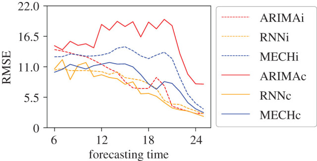
Root mean square error (RMSE) between predicted and real time series of incidence of dengue for intense outbreaks (dengue cases ≥200). ARIMAi, RNNi and MECHi are the results for models using only local dengue data, the baseline models, and ARIMAc, RNNc and MECHc are the results for the forecasts generated including human mobility data.
Figure 10 shows the results of average log scores for peak intensity, peak timing and the whole time-series prediction. With this metric, which evaluates the accuracy of the probabilistic forecast, the effect of the mobility data was less straightforward. Both types of models generally benefitted from the mobility data in forecasting peak timing. However, the inclusion of the mobility data led to lower log scores for peak timing, and at certain times, for the time series of future dengue incidence. For peak intensity, the mechanistic model shows more consistent results presenting higher values for both local and network prediction. The neural network models clearly show better results for peak timing prediction based on MAE and log score. This result also holds for prediction of entire time series.
Figure 10.

Log-score results for peak intensity (a), peak timing (b) and dengue time series (c) for outbreaks with total number of dengue cases greater than 200.
We tested the sensitivity of our analysis to the choice of 200 cases as the neighbourhood level epidemic threshold. We evaluated the models’ ability to predict dengue cases in a period with dengue cases greater than 100 and greater than 300. The results strengthen the findings of our main analysis: the mechanistic model better predicts large epidemics, but overestimates periods when there are fewer dengue cases, and the neural network model continues to better predict peak timing in all analyses. The epidemic threshold analyse electronic supplementary material describes in more detail the epidemic threshold analysis.
In order to understand the reasons the neural network model obtained better results using vector representations of the network of people flow in the prediction of the time series as a whole (figure 9) and in the prediction of peak intensity of dengue cases (figure 8a), we decided to investigate more deeply the spatio-temporal scenario.
Figure 11 shows the spatial distribution of RMSE for forecasts made using the RNNc model during epidemic years. In these years, the RMSE for neighbourhoods in the west of the city (left side) is lower. This region is made up of the most populated neighbourhoods with the highest poverty indicators. The figures presented in ‘appearance of dengue electronic supplementary material’ indicate that the west of the city is the region where dengue cases first appear in peak years. This suggests that the use of human mobility data is important for capturing the flow of the dengue virus from the west to the east of the city. Figure 12 shows that by using human mobility data there was reduced forecast error in neighbourhoods in the east, particularly for peak intensity and prediction of the time series as a whole.
Figure 11.

For each peak year of dengue cases (2008, 2011, 2012 and 2015) the RMSE for the LSTM networked model is represented as a colour scale for each neighbourhood.
Figure 12.

Test conducted for neighbourhoods in the western region. (a) Map illustrating the neighbourhoods that were considered in the tests, (b) MAE for peak intensity, (c) MAE for peak time and RMSE for time series as a whole.
The neighbourhoods with more accurate predictions are located in the west of the city, the most populous region and where the first cases of dengue occurred in peak years. This indicates that the neural network model performed better predicting incidence during the early stage of an outbreak with a clear growth trend. This outcome suggests a need to further strengthen understanding of the spread of dengue via human mobility data and better predict dengue cases in neighbourhoods other than those with such clear trends. At the same time, in the RNNc model there was an improvement in the forecast accuracy for neighbourhoods that were not in the western region, indicating that the neural network model was able to capture the spatio-temporal aspects of the dengue transmission.
4. Discussion and conclusion
In this paper, we proposed two distinct dengue forecasting systems and explored the use of human mobility data as a part of these forecasting systems. The first forecast system employed neural network architectures: one forecasting dengue cases using only local historical dengue data and the other one, embedding human mobility data, as well as past dengue data, into a hierarchical architecture. The second type of forecast system used a mechanistic model coupled with a data assimilation system. We presented an isolated version which using only local historical dengue data and a linked version which also incorporates human mobility data. Findings indicate that inclusion of human mobility data improves forecast accuracy for both the neural network and mechanistic models. Both methods can classify outbreak intensity, although the mechanistic models better capture large outbreaks. However, for forecast of the full dengue time series or identification of peak timing and intensity, the neural network models were more accurate. A comparison with a traditional ARIMA method was also performed. The ARIMA forecasting approach, as expected, produced less accurate forecasts because it was not able to capture the long-term dependency of historical dengue cases or the complex nonlinear relationship that presented in the mobility data.
Compared with mechanistic models, the neural networks, which here have more parameters and a more complex structure, are better able to capture a broader range of nonlinear transmission dynamics. This difference may explain why the neural network outperforms the mechanistic models in predicting dengue outbreak peak intensity and the incidence time series. Also it is important to mention that despite the good performance of the neural network forecasting systems, neural networks have disadvantages that must be considered. In particular, the neural network model requires a large amount of data and effort to adjust its hyper-parameters to prevent over-fitting. Thus, a high-performance computer is needed to cover the computational cost in training the models and to reduce the training time. To perform the tests for the local neural network model, each model for each neighbourhood was trained for 144 min for each forecasting week. In total, there were 20 different forecasting weeks, from week 6 to week 25, requiring 2880 min (48 h) to perform this test. However, it was less time consuming to perform the tests for the RNNc (i.e. including human mobility data). The architecture for this model allows for the prediction of dengue cases for all the neighbourhoods at once, thus reducing the training time to 3 h.
As with previous comparisons of different types forecasting systems [62,70,72], we found that the neural network system and the mechanistic system each outperformed the other for certain forecast targets and evaluation metrics. This indicates that a super-ensemble approach, in which forecasts produced using different methods are combined into weighted averages based on their historical performance, would be beneficial. A super-ensemble approach can also benefit from the ability of each system to consider different types of information, e.g. spatial, temporal, etc., as well as representing this information differently. For instance, one model can represent the spatial-dependency as a Node2Vec embedding while another model can represent this by means of a graph convolutional network [73]. Also, an ensemble might allow the models to be considered as basic features of the time-series and/or spatial properties. For example, an LSTM-model without spatial or transport data might produce better results for neighbourhoods with low movement.
The findings of this research open up new avenues for understanding the impact of urban mobility on the epidemic of diseases such as dengue in large cities as well as for understanding the adequacy and limitations of important forecast tools coming from different contexts such as neural nets and mechanistic models.
Supplementary Material
Supplementary Material
Supplementary Material
Supplementary Material
Data accessibility
Data and codes available are at https://github.com/rafaellpontes/dengue_mobility_paper.
Authors' contributions
R.B. and S.P. developed and implemented methods and generating forecasts. All authors were involved in designing the study and analysing results. R.B. and S.P. drafted the initial version of the manuscript and created visualizations. All authors reviewed and revised the manuscript and approve publication.
Competing interests
J.S. and Columbia University disclose partial ownership of SK Analytics. J.S. discloses consulting for BNI and Merck. S.P. and T.Y. declare no competing interests.
Funding
J.S., S.P. and T.Y. were supported by NIGMS grant no. GM110748, DARPA contract W911NF-16-2-0035 and a gift from the Morris-Singer Foundation. J.S.A.J. gratefully acknowledges financial support from the Brazilian agencies CNPq, CAPES, and FUNCAP. R.B. was supported by FUNCAP.
References
- 1.Bhatt S. et al. 2013. The global distribution and burden of dengue. Nature 496, 504–507. ( 10.1038/nature12060) [DOI] [PMC free article] [PubMed] [Google Scholar]
- 2.World Health Organization. Dengue and severe dengue. See https://www.who.int/news-room/fact-sheets/detail/dengue-and-severe-dengue (accessed 18 June 2019).
- 3.Gibbons RV, Vaughn DW. 2002. Dengue: an escalating problem. Brit. Med. J. 324, 1563–1566. ( 10.1136/bmj.324.7353.1563) [DOI] [PMC free article] [PubMed] [Google Scholar]
- 4. Instituto Brasileiro de Geografia e Estatistica (IBGE). See http://www.ibge.gov.br. (accessed 18 June 2019).
- 5.Oliveira RdMAB, Araújo FMdC, Cavalcanti LPdG. 2018. Aspectos entomológicos e epidemiológicos das epidemias de dengue em Fortaleza, Ceará, 2001–2012. Epidemiologia e Serviços de Saúde 27, e201704414 ( 10.5123/S1679-49742018000100014) [DOI] [PubMed] [Google Scholar]
- 6.MacCormack-Gelles B, Neto AS, Sousa GS, Nascimento OJ, Machado MM, Wilson ME, Castro MC. 2018. Epidemiological characteristics and determinants of dengue transmission during epidemic and non-epidemic years in Fortaleza, Brazil: 2011–2015. PLoS Negl. Trop. Dis. 12, e0006990 ( 10.1371/journal.pntd.0006990) [DOI] [PMC free article] [PubMed] [Google Scholar]
- 7.Braga IA, Valle D. 2007. Aedes aegypti: histórico do controle no Brasil. Epidemiologia e serviços de saúde 16, 113–118. ( 10.5123/S1679-49742007000400007) [DOI] [Google Scholar]
- 8.Garcia GD, David MR, Martins AD, Maciel-de-Freitas R, Linss JG, Araújo SC, Lima JB, Valle D. 2018. The impact of insecticide applications on the dynamics of resistance: the case of four Aedes aegypti populations from different Brazilian regions. PLoS Negl. Trop. Dis. 12, e0006227 ( 10.1371/journal.pntd.0006227) [DOI] [PMC free article] [PubMed] [Google Scholar]
- 9.Neto ASL, de Sousa GdS. 2016. Dengue, zika e chikungunya—desafios do controle vetorial frente à ocorrência das três arboviroses—parte I. Revista Brasileira em Promoção da Saúde 29, 305–312. ( 10.5020/18061230.2016.p305) [DOI] [Google Scholar]
- 10.Neto ASL, de Sousa GdS, de Oliveira Lima JW. 2016. Dengue, zika e chikungunya—desafios do controle vetorial frente à ocorrência das três arboviroses—parte II. Revista Brasileira em Promoção da Saúde 29, 463–465. ( 10.5020/18061230.2016.p463) [DOI] [Google Scholar]
- 11.Van Panhuis WG. et al. 2015. Region-wide synchrony and traveling waves of dengue across eight countries in Southeast Asia. Proc. Natl Acad. Sci. USA 112, 13 069–13 074. ( 10.1073/pnas.1501375112) [DOI] [PMC free article] [PubMed] [Google Scholar]
- 12.Guo P. et al. 2017. Developing a dengue forecast model using machine learning: a case study in China. PLoS Negl. Trop. Dis. 11, e0005973 ( 10.1371/journal.pntd.0005973) [DOI] [PMC free article] [PubMed] [Google Scholar]
- 13.Yusof Y, Mustaffa Z. 2011. Dengue outbreak prediction: a least squares support vector machines approach. Int. J. Comput. Theory Eng. 3, 489 ( 10.7763/IJCTE.2011.V3.355) [DOI] [Google Scholar]
- 14.Souza RC, Assunção RM, Oliveira DM, Neill DB, Meira W Jr. 2019. Where did I get dengue? Detecting spatial clusters of infection risk with social network data. Spatial and Spatio-Temporal Epidemiol. 29, 163–175. ( 10.1016/j.sste.2018.11.005) [DOI] [PubMed] [Google Scholar]
- 15.Sanna M, Hsieh YH. 2017. Ascertaining the impact of public rapid transit system on spread of dengue in urban settings. Sci. Total Environ. 598, 1151–1159. ( 10.1016/j.scitotenv.2017.04.050) [DOI] [PMC free article] [PubMed] [Google Scholar]
- 16.Kraemer MU. et al. 2018. Inferences about spatiotemporal variation in dengue virus transmission are sensitive to assumptions about human mobility: a case study using geolocated tweets from Lahore, Pakistan. EPJ Data Sci. 7, 16 ( 10.1140/epjds/s13688-018-0144-x) [DOI] [PMC free article] [PubMed] [Google Scholar]
- 17.Aguas R, Dorigatti I, Coudeville L, Luxemburger C, Ferguson N. 2019. Cross-serotype interactions and disease outcome prediction of dengue infections in Vietnam. Sci. Rep. 9, 9395 ( 10.1038/s41598-019-45816-6) [DOI] [PMC free article] [PubMed] [Google Scholar]
- 18.Nan J, Liao X, Chen J, Chen X, Chen J, Dong G, Liu K, Hu G. 2018. Using climate factors to predict the outbreak of dengue fever. In 2018 7th Int. Conf. on Digital Home (ICDH), pp. 213–218. New York, NY: IEEE.
- 19.Kesorn K, Ongruk P, Chompoosri J, Phumee A, Thavara U, Tawatsin A, Siriyasatien P. 2015. Morbidity rate prediction of dengue hemorrhagic fever (DHF) using the support vector machine and the Aedes aegypti infection rate in similar climates and geographical areas. PLoS ONE 10, e0125049 ( 10.1371/journal.pone.0125049) [DOI] [PMC free article] [PubMed] [Google Scholar]
- 20.Husin NA. et al. 2008. Modeling of dengue outbreak prediction in Malaysia: a comparison of neural network and nonlinear regression model. In 2008 Int. Symp. on Information Technology, vol. 3, pp. 1–4. New York, NY: IEEE.
- 21.Osthus D, Gattiker J, Priedhorsky R, Del Valle SY. 2019. Dynamic bayesian influenza forecasting in the united states with hierarchical discrepancy (with discussion). Bayesian Anal. 14, 261–312. ( 10.1214/18-BA1117) [DOI] [Google Scholar]
- 22.Shaman J, Yang W, Kandula S. 2014. Inference and forecast of the current West African Ebola outbreak in Guinea, Sierra Leone and Liberia. PLoS Curr. 6, ecurrents.outbreaks.3408774290b1a0f2dd7cae877c8b8ff6. ( 10.1371/currents.outbreaks.3408774290b1a0f2dd7cae877c8b8ff6) [DOI] [PMC free article] [PubMed] [Google Scholar]
- 23.DeFelice NB, Little E, Campbell SR, Shaman J. 2017. Ensemble forecast of human West Nile virus cases and mosquito infection rates. Nat. Commun. 8, 14592 ( 10.1038/ncomms14592) [DOI] [PMC free article] [PubMed] [Google Scholar]
- 24.Johansson MA. et al. 2019. An open challenge to advance probabilistic forecasting for dengue epidemics. Proc. Natl Acad. Sci. 116, 24 268–24 274. ( 10.1073/pnas.1909865116) [DOI] [PMC free article] [PubMed] [Google Scholar]
- 25.Yamana TK, Kandula S, Shaman J. 2016. Superensemble forecasts of dengue outbreaks. J. R. Soc. Interface 13, 20160410 ( 10.1098/rsif.2016.0410) [DOI] [PMC free article] [PubMed] [Google Scholar]
- 26.Kuno G. 1995. Review of the factors modulating dengue transmission. Epidemiol. Rev. 17, 321–335. ( 10.1093/oxfordjournals.epirev.a036196) [DOI] [PubMed] [Google Scholar]
- 27.Stoddard ST. et al. 2013. House-to-house human movement drives dengue virus transmission. Proc. Natl Acad. Sci. USA 110, 994–999. ( 10.1073/pnas.1213349110) [DOI] [PMC free article] [PubMed] [Google Scholar]
- 28.Vazquez-Prokopec GM, Montgomery BL, Horne P, Clennon JA, Ritchie SA. 2017. Combining contact tracing with targeted indoor residual spraying significantly reduces dengue transmission. Sci. Adv. 3, e1602024 ( 10.1126/sciadv.1602024) [DOI] [PMC free article] [PubMed] [Google Scholar]
- 29.Salje H. et al. 2017. Dengue diversity across spatial and temporal scales: local structure and the effect of host population size. Science 355, 1302–1306. ( 10.1126/science.aaj9384) [DOI] [PMC free article] [PubMed] [Google Scholar]
- 30.Adams B, Kapan DD. 2009. Man bites mosquito: understanding the contribution of human movement to vector-borne disease dynamics. PLoS ONE 4, e6763 ( 10.1371/journal.pone.0006763) [DOI] [PMC free article] [PubMed] [Google Scholar]
- 31.Barmak DH, Dorso CO, Otero M, Solari HG. 2011. Dengue epidemics and human mobility. Phys. Rev. E 84, 011901 ( 10.1103/PhysRevE.84.011901) [DOI] [PubMed] [Google Scholar]
- 32.Wen TH, Lin MH, Fang CT. 2012. Population movement and vector-borne disease transmission: differentiating spatial–temporal diffusion patterns of commuting and noncommuting dengue cases. Ann. Assoc. Am. Geogr. 102, 1026–1037. ( 10.1080/00045608.2012.671130) [DOI] [Google Scholar]
- 33.Guzzetta G, Marques-Toledo CA, Rosà R, Teixeira M, Merler S. 2018. Quantifying the spatial spread of dengue in a non-endemic Brazilian metropolis via transmission chain reconstruction. Nat. Commun. 9, 2837 ( 10.1038/s41467-018-05230-4) [DOI] [PMC free article] [PubMed] [Google Scholar]
- 34.Antonio FJ, Itami AS, de Picoli S, Teixeira JJV. 2017. Spatial patterns of dengue cases in Brazil. PLoS ONE 12, e0180715 ( 10.1371/journal.pone.0180715) [DOI] [PMC free article] [PubMed] [Google Scholar]
- 35.Siqueira JB. et al. 2004. Household survey of dengue infection in central Brazil: spatial point pattern analysis and risk factors assessment. Am. J. Trop. Med. Hyg. 71, 646–651. ( 10.4269/ajtmh.2004.71.646) [DOI] [PubMed] [Google Scholar]
- 36.Souza RC, Neill DB, Assunção RM, Meira W. 2019. Identifying high-risk areas for dengue infection using mobility patterns on twitter. Online J. Public Health Inform. 11, e246 ( 10.5210/ojphi.v11i1.9754) [DOI] [Google Scholar]
- 37.Lana RM, de Lima TFM, Honório NA, Codeço CT. 2017. The introduction of dengue follows transportation infrastructure changes in the state of Acre, Brazil: a network-based analysis. PLoS Negl. Trop. Dis. 11, e0006070 ( 10.1371/journal.pntd.0006070) [DOI] [PMC free article] [PubMed] [Google Scholar]
- 38.Chen Y, Ong JHY, Rajarethinam J, Yap G, Ng LC, Cook AR. 2018. Neighbourhood level real-time forecasting of dengue cases in tropical urban Singapore. BMC Med. 16, 129 ( 10.1186/s12916-018-1108-5) [DOI] [PMC free article] [PubMed] [Google Scholar]
- 39.Tibshirani R. 1996. Regression shrinkage and selection via the lasso. J. R. Stat. Soc.: Ser. B (Methodological) 58, 267–288. ( 10.1111/j.2517-6161.1996.tb02080.x) [DOI] [Google Scholar]
- 40.Wesolowski A, Qureshi T, Boni MF, Sundsøy PR, Johansson MA, Rasheed SB, Engø–Monsen K, Buckee CO. 2015. Impact of human mobility on the emergence of dengue epidemics in Pakistan. Proc. Natl Acad. Sci. USA 112, 11887–11892. ( 10.1073/pnas.1504964112) [DOI] [PMC free article] [PubMed] [Google Scholar]
- 41.Sistema de Monitoramento Diário de Agravos (SIMDA);. See http://tc1.sms.fortaleza.ce.gov.br/simda (accessed 18 June 2019).
- 42.Caminha C, Furtado V, Pequeno TH, Ponte C, Melo HP, Oliveira EA, Andrade JS Jr. 2017. Human mobility in large cities as a proxy for crime. PLoS ONE 12, e0171609 ( 10.1371/journal.pone.0171609) [DOI] [PMC free article] [PubMed] [Google Scholar]
- 43.Caminha C, Furtado V, Pinheiro V, Silva C. 2016. Micro-interventions in urban transportation from pattern discovery on the flow of passengers and on the bus network. In 2016 IEEE Int. Smart Cities Conf. (ISC2), pp. 1–6. New York, NY: IEEE.
- 44.Caminha C, Furtado V. 2017. Impact of human mobility on police allocation. In 2017 IEEE Int. Conf. on Intelligence and Security Informatics (ISI), pp. 125–127. New York, NY: IEEE.
- 45.Sullivan D, Caminha C, Melo HP, Furtado V. 2017. Towards understanding the impact of crime on the choice of route by a bus passenger. In EPIA Conf. on Artificial Intelligence, pp. 41–50. Berlin, Germany: Springer.
- 46.Ponte C, Caminha C, Furtado V. 2016. Busca de melhor caminho entre dois pontos quando múltiplas origens e múltiplos destinos são possíveis. In XIII National Meeting on Artificial and Computational Intelligence - ENIAC'2016, Recife, Brazil, 9–12 October.
- 47.Furtado V, Furtado E, Caminha C, Lopes A, Dantas V, Ponte C, Cavalcante S. 2017. A data-driven approach to help understanding the preferences of public transport users. In 2017 IEEE Int. Conf. on Big Data (Big Data), pp. 1926–1935. New York, NY: IEEE.
- 48.Caminha C, Furtado V, Pinheiro V, Ponte C. 2018. Graph mining for the detection of overcrowding and waste of resources in public transport. J. Internet Services Appl. 9, 22 ( 10.1186/s13174-018-0094-3) [DOI] [Google Scholar]
- 49.Elman JL. 1990. Finding structure in time. Cogn. Sci. 14, 179–211. ( 10.1207/s15516709cog1402_1) [DOI] [Google Scholar]
- 50.Hochreiter S, Schmidhuber J. 1997. Long short-term memory. Neural Comput. 9, 1735–1780. ( 10.1162/neco.1997.9.8.1735) [DOI] [PubMed] [Google Scholar]
- 51.Gal Y, Ghahramani Z. 2016. Dropout as a bayesian approximation: representing model uncertainty in deep learning. In Proc. of the 33rd Int. Conf. on Machine Learning. PMLR 48, 1050–1059. [Google Scholar]
- 52.Bontempi G, Taieb SB, Le Borgne YA. 2012. Machine learning strategies for time series forecasting. In European business intelligence summer school, pp. 62–77. Berlin, Germany: Springer.
- 53.Taieb SB, Hyndman RJ. 2012. Recursive and direct multi-step forecasting: the best of both worlds. Monash Econometrics and Business Statistics Working Papers 19/12, Monash University, Department of Econometrics and Business Statistics. See https://www.monash.edu/business/ebs/research/publications/ebs/wp19-12.pdf. [Google Scholar]
- 54.Grover A, Leskovec J. 2016. node2vec: Scalable feature learning for networks. In Proc. of the 22nd ACM SIGKDD Int. Conf. on Knowledge discovery and data mining, pp. 855–864. New York, NY: ACM.
- 55.Mikolov T, Chen K, Corrado G, Dean J. 2013 Efficient estimation of word representations in vector space. arXiv (http://arxiv.org/abs/13013781. )
- 56.Shaman J, Karspeck A. 2012. Forecasting seasonal outbreaks of influenza. Proc. Natl Acad. Sci. USA 109, 20 425–20 430. ( 10.1073/pnas.1208772109) [DOI] [PMC free article] [PubMed] [Google Scholar]
- 57.Shaman J, Karspeck A, Yang W, Tamerius J, Lipsitch M. 2013. Real-time influenza forecasts during the 2012–2013 season. Nat. Commun. 4, 2837 ( 10.1038/ncomms3837) [DOI] [PMC free article] [PubMed] [Google Scholar]
- 58.Pei S, Shaman J. 2017. Counteracting structural errors in ensemble forecast of influenza outbreaks. Nat. Commun. 8, 925 ( 10.1038/s41467-017-01033-1) [DOI] [PMC free article] [PubMed] [Google Scholar]
- 59.Yang W, Lipsitch M, Shaman J. 2015. Inference of seasonal and pandemic influenza transmission dynamics. Proc. Natl Acad. Sci. USA 112, 2723–2728. ( 10.1073/pnas.1415012112) [DOI] [PMC free article] [PubMed] [Google Scholar]
- 60.Pei S, Cane MA, Shaman J. 2019. Predictability in process-based ensemble forecast of influenza. PLoS Comput. Biol. 15, e1006783 ( 10.1371/journal.pcbi.1006783) [DOI] [PMC free article] [PubMed] [Google Scholar]
- 61.Yang W. et al. 2015. Transmission network of the 2014–2015 Ebola epidemic in Sierra Leone. J. R. Soc. Interface 12, 20150536 ( 10.1098/rsif.2015.0536) [DOI] [PMC free article] [PubMed] [Google Scholar]
- 62.Kandula S, Yamana T, Pei S, Yang W, Morita H, Shaman J. 2018. Evaluation of mechanistic and statistical methods in forecasting influenza-like illness. J. R. Soc. Interface 15, 20180174 ( 10.1098/rsif.2018.0174) [DOI] [PMC free article] [PubMed] [Google Scholar]
- 63.Pei S, Morone F, Liljeros F, Makse H, Shaman JL. 2018. Inference and control of the nosocomial transmission of methicillin-resistant Staphylococcus aureus. eLife 7, e40977 ( 10.7554/eLife.40977) [DOI] [PMC free article] [PubMed] [Google Scholar]
- 64.Anderson JL. 2001. An ensemble adjustment Kalman filter for data assimilation. Mon. Weather Rev. 129, 2884–2903. ( 10.1175/1520-0493(2001)12960;2884:AEAKFF62;2.0.CO;2) [DOI] [Google Scholar]
- 65.Pei S, Kandula S, Yang W, Shaman J. 2018. Forecasting the spatial transmission of influenza in the United States. Proc. Natl Acad. Sci. USA 115, 2752–2757. ( 10.1073/pnas.1708856115) [DOI] [PMC free article] [PubMed] [Google Scholar]
- 66.Box GE, Jenkins GM, Reinsel GC, Ljung GM. 2015. Time series analysis: forecasting and control. New York, NY: John Wiley & Sons. [Google Scholar]
- 67.Ariyo AA, Adewumi AO, Ayo CK. 2014. Stock price prediction using the ARIMA model. In 2014 UKSim-AMSS 16th Int. Conf. on Computer Modelling and Simulation, pp. 106–112. New York, NY: IEEE.
- 68.Rahman M, Islam AS, Nadvi SYM, Rahman RM. 2013. Comparative study of ANFIS and ARIMA model for weather forecasting in Dhaka. In 2013 Int. Conf. on Informatics, Electronics and Vision (ICIEV), pp. 1–6. New York, NY: IEEE.
- 69.He Z, Tao H. 2018. Epidemiology and ARIMA model of positive-rate of influenza viruses among children in Wuhan, China: a nine-year retrospective study. Int. J. Infect. Dis. 74, 61–70. ( 10.1016/j.ijid.2018.07.003) [DOI] [PubMed] [Google Scholar]
- 70.Reich NG. et al. 2019. A collaborative multiyear, multimodel assessment of seasonal influenza forecasting in the United States. Proc. Natl Acad. Sci. USA 116, 3146–3154. ( 10.1073/pnas.1812594116) [DOI] [PMC free article] [PubMed] [Google Scholar]
- 71.Biggerstaff M. et al. 2018. Results from the second year of a collaborative effort to forecast influenza seasons in the United States. Epidemics 24, 26–33. ( 10.1016/j.epidem.2018.02.003) [DOI] [PMC free article] [PubMed] [Google Scholar]
- 72.Yamana TK, Kandula S, Shaman J. 2017. Individual versus superensemble forecasts of seasonal influenza outbreaks in the United States. PLoS Comput. Biol. 13, e1005801 ( 10.1371/journal.pcbi.1005801) [DOI] [PMC free article] [PubMed] [Google Scholar]
- 73.Kipf TN, Welling M. 2016 Semi-supervised classification with graph convolutional networks. arXiv (http://arxiv.org/abs/160902907. )
Associated Data
This section collects any data citations, data availability statements, or supplementary materials included in this article.
Supplementary Materials
Data Availability Statement
Data and codes available are at https://github.com/rafaellpontes/dengue_mobility_paper.