Neutral components show a hierarchical community structure in the genotype–phenotype map of RNA secondary structure

Abstract

Genotype–phenotype (GP) maps describe the relationship between biological sequences and structural or functional outcomes. They can be represented as networks in which genotypes are the nodes, and one-point mutations between them are the edges. The genotypes that map to the same phenotype form subnetworks consisting of one or multiple disjoint connected components–so-called neutral components (NCs). For the GP map of RNA secondary structure, the NCs have been found to exhibit distinctive network features that can affect the dynamical processes taking place on them. Here, we focus on the community structure of RNA secondary structure NCs. Building on previous findings, we introduce a method to reveal the hierarchical community structure solely from the sequence constraints and composition of the genotypes that form a given NC. Thereby, we obtain modularity values similar to common community detection algorithms, which are much more complex. From this knowledge, we endorse a sampling method that allows a fast exploration of the different communities of a given NC. Furthermore, we introduce a way to estimate the community structure from genotype samples, which is useful when an exhaustive analysis of the NC is not feasible, as is the case for longer sequence lengths.

1. Introduction

The mapping between genotypes and phenotypes can be understood as a network, and can therefore be analysed using the tools of network science. The fundamental idea [1–3] is to consider the space of all genotype sequences—for example, all RNA, DNA or amino acid sequences of a given fixed length—as a network, in which each sequence is represented by a node and each one-point mutation between two genotypes by an edge. Genotypes that map to the same phenotype have been shown to be correlated [4] and to form subnetworks. These subnetworks—commonly referred to as neutral sets or neutral networks—are either fully connected or consist of multiple disjoint components—commonly referred to as neutral components (NCs). One-point mutations between genotypes in an NC do not change the phenotype (and therefore the fitness) and are labelled as neutral. By contrast, mutations between genotypes of disjoint NCs of the same phenotype can involve genotypes with phenotypes of lower fitness, meaning unfavourable steps from an evolutionary perspective. Thus, in this article, we will focus on NCs—the most essential neutral units for evolving populations on the genotype space.

One of the most extensively studied genotype–phenotype (GP) maps is the mapping between RNA sequences (genotypes) and their secondary structure (phenotypes) [4–13]. The secondary structure is an abstraction of the full three-dimensional spatial structure and only considers the base pair configuration—often shown using the ‘dot–bracket notation’. If we compare the set of genotypes that belong to a given NC, the unpaired sequence sites tend to be the most unconstrained, meaning that they allow a significant number of neutral mutations so that a range of different letters (nucleotides) can be found at each of these sites. By contrast, the paired sites are mostly constrained and only allow a limited number of neutral mutations so that only a limited range of different letters is found at each of these sites.

Aguirre et al. [9] were the first to thoroughly analyse the topological properties of the NCs of the RNA secondary structure GP map of sequence length L = 12. Among other unique properties, they showed that the NC networks are assortative and exhibit a community structure. For an example NC, they studied the community structure by comparing the degree of the nodes with their eigenvector centrality. In this context, they discovered that these communities can be characterized by the letter combinations at the base pairs in the stacks of the respective phenotype [9]. Capitán et al. [14] continued this research and further studied the community structure of RNA secondary structure NCs. Using another example NC, they identified ‘dynamical communities’ and a hierarchical community structure by running population dynamics on the NC. In particular, they studied the equilibrium distribution—related to the eigenvectors of the adjacency matrix also considered in [9]—as well as the time to equilibrium distribution. Their findings confirmed that the identified communities can be characterized by letter combinations at certain sequence sites, in this case at two unpaired sites, since the paired sites are fully constrained for the considered example NC. A further study of the topological properties of NCs can be found in the PhD thesis by Greenbury [15]. Studying the GP maps of RNA secondary structure and of the so-called Polyomino model [12,16], this work also draws links between the community structure of an NC and the sequence constraints and composition of the genotype sequences that form this NC. Building on empirical data, Aguilar-Rodríguez et al. [17] studied the architecture—including the community structure—of genotype networks in the GP map of transcription factor binding sites. Studies on the impact of topological properties of NCs on population dynamics range from initial work by van Nimwegen et al. [18] to more recent studies by Manrubia and co-workers [19,20].

In this article, we present a method that reveals the hierarchical community structure of an NC solely from the sequence constraints and composition of its genotypes, without the necessity of running complex community detection algorithms. In the first instance, this approach is designed to reveal the community structure of NCs that are fully mapped, meaning that we know all their constituent sequences. However, we also introduce a way to estimate the community structure from genotype samples of the full NC. Here, we only consider the RNA secondary structure GP map, but our framework could potentially be adapted to many other GP maps.

As the main model system, we use the RNA secondary structure GP map of sequence length L = 12, for which the NCs have a size that allows meaningful plots of the NC networks as well as a network analysis in a reasonable computational time. To predict the secondary structure of a given RNA sequence, we use the Python implementation of the so-called ViennaRNA package [21–23] (v. 2.4.9, default parameters) with its function RNA.fold. There are 431 NCs (ignoring the undefined phenotype, or unbound structure), which we rank with respect to their size, with the largest receiving rank 1. For the network analysis, we mainly use the Python package NetworkX.

The article is structured as follows. We start by explaining our method to reveal the hierarchical community structure of an NC and apply it to the NCs of the L = 12 RNA secondary structure GP map. This is followed by the endorsement of a sampling method that allows a fast exploration of the different NC communities. Finally, using this method, we introduce a way to estimate the community structure from samples of genotypes. We apply it to two NCs that comprise naturally occurring functional non-coding RNA sequences of longer lengths.

2. Sequence-based communities

We begin by introducing our method to reveal the hierarchical communities of the NCs that can be applied whenever the NC of interest is fully known.

2.1. Method

The starting point is the number of neutral mutations per sequence site averaged over the NC—a measure of the average constraint of sequence sites across the genotypes of the NC. For an individual genotype, the number of neutral mutations for a particular site measures how many different letters the current letter at this site can be mutated to without changing the phenotype. For RNA with its four-letter alphabet, it ranges from 0 (fully constrained) to 3 (fully unconstrained).

In order to reveal the communities, we consider all sites, starting with the most constrained (smallest average number of neutral mutations) and moving to the least constrained (largest average number of neutral mutations). We exclude fully constrained sites (zero average number of neutral mutations) as all genotypes of the NC have the same letters at these sites. We begin with an empty list of constrained positions and add to this list the position of the most constrained site with non-zero average number of neutral mutations. Next, we go through the genotypes of the NC and associate them with communities according to the letters that they have at these positions. In other words, the different communities are defined by different letter combinations at the constrained positions and genotypes belong to the same community if they have the same letters at these positions. Once all genotypes of the NC have been considered, we add the position of the next most constrained site to our list of constrained positions and repeat the procedure until we have added the positions of all sites. Whenever multiple sites have exactly the same average number of neutral mutations, we add their positions in the same step. Figure 1 illustrates the procedure.

Figure 1.

Depiction of the sequence-based communities method applied to four example NCs of the L = 12 RNA secondary structure GP map: (a) NC of rank 32 (size: 19 488, secondary structure: ‘(((… .))). .’, (b) 36 (size: 18 468, ‘.((… .))…’, (c) 41 (size: 16 815, ‘.(((…))). .’, and (d) 94 (size: 7341, ‘((((… .))))’). In each of the four cases, at the top, the average number of neutral mutations per site averaged over all genotypes of the NC is displayed. The crosses indicate fully constrained sites (zero average number of neutral mutations). The shaded grey areas highlight paired sites. The numbers indicate the ordering of the sites according to their constraint (average number of neutral mutations), with the site having the smallest non-zero average number of neutral mutations receiving number 1 and so on. If sites have exactly the same constraint, they receive the same number. In each case, underneath the top figure, for a range of steps, the full NC network with coloured communities, its modularity Q and its coarse-grained network representation are shown, respectively, according to associating the communities with letter combinations at the positions of the sites with a number up to and including the respective step number. Both the full and coarse-grained networks are plotted using a force-directed graph layout algorithm. In addition, if the coarse-grained networks are not too large, the associated letter combinations are shown. The red step numbers and modularity values indicate the respective step that leads to the community structure with maximum modularity. The examples demonstrate that the community structure of an NC can be revealed by considering the sites in order of their decreasing constraint levels. Larger decreases in the constraint are associated with a change in the hierarchy layer.

This association of communities with letter combinations at constrained positions is similar to how Manrubia and co-workers characterize the communities for two individual RNA secondary structure NCs in [9] (letter combinations at paired sites) and [14] (letter combinations at constrained unpaired sites while the paired sites are fully constrained). Our method unifies these ideas, as well as the idea by Greenbury [15] to relate sequence constraints and composition to the community division of an NC, by providing a simple algorithm that can be applied to any fully known NC.

For every step in our method, we calculate the modularity of the discovered community structure. The concept of modularity in this context was introduced by Newman and Girvan [24,25] and measures whether the sets of nodes in a given partition are more densely connected inside each set than one would expect by chance. The modularity Q is calculated by [24,25]

$$Q=\sum _i(e_{ii}-a_i^2),$$ 2.1

where the sum runs over all communities. e_ii measures the fraction of all ends of edges that are attached with both ends to nodes in community i and a_i measures the fraction of all ends of edges that are attached to nodes in community i [24,25]. The contribution of a given community i to the modularity is therefore positive if e_ii is greater than the null expectation $a_i^2$. The higher the modularity (which ranges from −1 to 1), the more meaningful a community division.

With each step in our procedure, a finer-grained community structure is revealed. At a fully constrained site, there can be only one letter. For RNA, if a site with a non-zero average number of neutral mutations is unpaired, in principle, there can be four different letters; if it is paired, two different letters; and for two sites corresponding to the same base pair, three different letter combinations. This sets an upper limit for the number of communities that are possible in principle. Therefore, it is to be expected that the modularity initially will increase when adding more sites to the list of constrained positions, will reach a maximum that corresponds to the most meaningful community structure, and then will decrease as the community structures become too fine-grained.

The association of communities with letter combinations at constrained positions also allows a coarse-grained network representation of the full NC topology. We simply associate a given letter combination with a coarse-grained node and connect two coarse-grained nodes whenever the associated letter combinations differ by only one letter. We choose the relative size of a coarse-grained node according to the number of genotypes within the respective community. There are a few caveats, as follows. Firstly, nodes in the original NC network with the same letter combinations at the constrained positions and therefore within the same community might not be fully connected, which is not reflected by representing all of them by one coarse-grained node. Secondly, there might not be any connection between nodes in the original NC network corresponding to two different coarse-grained nodes, even if the associated letter combinations at the constrained positions differ by only one letter. If necessary, this issue could be resolved by referring to the edges in the original NC network.

2.2. Examples

In the following, with figure 1, we explain the method using four example NCs from the L = 12 GP map that highlight different cases in a particularly clear way. For all examples, we show the average number of neutral mutations per site as well as for several steps of the method, the NC network with coloured communities, its modularity, its coarse-grained representation, and in some cases the associated letter combinations at the constrained positions. Both the full and the coarse-grained networks are plotted using a force-directed graph layout algorithm.

The first example in figure 1a is the NC of rank 32 with a phenotype that has three base pairs. The force-directed layout shows a clear community structure and suggests the presence of seven distinct communities. The two sites corresponding to the outermost base pair are the most constrained. In addition, they have the same constraint. Therefore, both positions are considered in the first step. At these two positions, we find three different letter combinations: the two Watson–Crick base pairs CG and UA and a wobble base pair UG connecting both. This means that we reveal three communities at this step. In the second step, we add the positions of the two sites corresponding to the innermost base pair, which again have the same constraint. At these four positions, we find five letter combinations, i.e. five communities. After the fourth step, the positions of all paired sites are added and we reveal seven communities exactly matching those that the force-directed layout suggests. The central community corresponds to three CG or GC base pairs, the most stable base pairs. The three communities adjacent to it correspond to letter combinations where one of those base pairs is exchanged for a UG or GU wobble base pair. Adjacent to each of these three communities, respectively, there is a community corresponding to a letter combination where the wobble base pair is exchanged for a UA or AU base pair. In the fifth step, the position of an unpaired site is added, which corresponds to a significant decrease in the constraint (increase in the average number of neutral mutations). We find that each of the communities from the previous step splits into three or four subcommunities—a new hierarchy layer. We stop at this step as further steps would simply lead to even more fine-grained and less meaningful community structures. This example shows how hierarchy layers are related to the site constraints. Sites that have a roughly similar constraint create a particular layer in a hierarchy. Adding the position of one of these sites progressively builds up such a layer, as we see here until step 4. A significant decrease in the constraint of an added site reflects a change in the hierarchical layer, as we see here for step 5. As already suggested by the force-directed layout, the maximum modularity is reached for step 4, though it only slightly decreases for steps 3 and 5, but then further beyond that.

The second example in figure 1b is the NC of rank 36, which corresponds to a two base pair phenotype. All paired sites are fully constrained and all genotypes have the same letters at these positions. In the first two steps, we add the positions of two unpaired sites that are roughly similarly constrained. We find 10 different letter combinations, and the communities match with the force-directed layout. The communities are less pronounced in the layout, probably because the unpaired sites considered here are less constrained than the paired sites considered in the previous example. In the third step, the position of a significantly less constrained site is added. This leads to an observable change in the hierarchy layer as explained. The maximum modularity is found for step 2 and slightly decreases for step 3, but does so more significantly for further steps. This NC and the community structure for step 2 resemble the example discussed in [14].

The third example in figure 1c nicely displays two observable changes in the hierarchy layer. It is the NC of rank 41 with a phenotype that has three base pairs. In contrast to the first example, two of the unpaired sites are significantly more constrained than the other ones, meaning three clusters of sites: six roughly similarly constrained paired sites, two roughly similarly half-constrained unpaired sites and four roughly similarly unconstrained unpaired sites. As explained, an observable change in the hierarchy layer occurs for steps 5 and 7, i.e. whenever the position of a site from a new cluster is added; in other words, when there is a significant change in the average number of neutral mutations. For step 4, we discover seven communities like those in step 4 in the first example. For step 6, we find 70 communities, which still largely mirror the organization of the nodes in the force-directed layout. The maximum modularity is found for step 5, which is only slightly larger than the modularity found for step 4.

Finally, in the fourth example in figure 1d, the NC of rank 94 is considered, which corresponds to a phenotype with four base pairs. For this example, we only show two steps as the principles are the same as before. After the fifth step, the positions of all roughly similarly constrained paired sites are added and the hierarchy layer is fully built up and matches the force-directed layout. The step afterwards leads to a change in the hierarchy layer and to a less relevant fine-grained community structure. The maximum modularity is reached for step 4, but is only slightly larger than for step 5.

2.3. Modularity comparison

Next, we benchmark our method in terms of the maximum modularity values against two common community detection algorithms in network science. For this, we consider all of the 200 largest NCs of the L = 12 GP map, which cover about 95% of the genotypes with a defined phenotype. We use this restriction since these NCs are reasonably large for a meaningful community analysis, though the exact threshold of 200 is arbitrary.

In figure 2, for these NCs, the maximum modularity values by our method are shown versus the modularity values provided by the Louvain and spin-glass algorithms, respectively. The Louvain algorithm [26] is a heuristic community detection algorithm built on an optimization of the modularity [26]. The spin-glass algorithm [27] uses a statistical mechanics approach and associates the community structure with an energy-minimizing spin configuration [27]. It is also one of the algorithms considered in [14] to find the ‘topological communities’ of the considered example NC. This algorithm is not part of the Python package NetworkX but the package igraph (also referred to as python-igraph), which we use in this case (v. 0.7.1).

Figure 2.

Maximum modularity values Q_max by our sequence-based communities method versus the modularity values Q by two common community detection algorithms: (a) Louvain (Q_L) and (b) spin-glass (Q_S) algorithm, for the 200 largest NCs of the L = 12 RNA secondary structure GP map. The coloured dots indicate the number of base pairs in the phenotypes corresponding to the NCs. Our method reveals community structures of modularity similar to or larger than the Louvain algorithm, and of modularity similar to the spin-glass algorithm.

In comparison with the Louvain algorithm, our method reveals community structures with modularity values that are roughly equal or larger (for small values). Compared with the spin-glass algorithm, there is great agreement in the modularity values. This proves that our simple method is able to find meaningful community structures in RNA secondary structure NCs as well as two much more complex community detection algorithms. It should be noted that the communities found by the Louvain and spin-glass algorithms do not (exactly) match those found by our method—an issue that is also discussed in [14].

3. Fast community sampling

Below, we will introduce a method to estimate the community structure of an NC from samples of genotypes in cases when the full NC is unknown. A prerequisite for this is the ability to generate a genotype sample that spaciously covers the NC. This means that a sampling method is required that can explore the different communities in a fast way. Recently, we introduced a method to estimate the size and robustness of NCs from small samples [28]. In this context, we developed a sampling method that we refer to as ‘site scanning sampling’, which proved to perform significantly better than a simple random walk (RW) sampling [28]. Here, building on our understanding of the community structure, we will discuss the reasoning behind this method in more detail and will again benchmark it against RW sampling.

3.1. Methods

As described in [28], RW sampling starts with a random genotype on the NC and tests random one-point mutations, i.e. we randomly select a site and randomly select a letter to which the letter at this site is mutated. If the mutation is neutral, the mutated genotype is added to the sample and serves as the new starting point; otherwise, a new random one-point mutation is tested. We repeat this procedure until a sample of designated size S is reached. Since random mutations of less constrained sites are more likely to be neutral than random mutations of more constrained sites, we know from our knowledge of the NC community structure that RW sampling favours a walk within communities, rather than between them. Already by definition, RWs on networks are biased towards higher degree nodes [29]. RWs and population dynamics resembling a RW on NCs of the RNA secondary structure GP map have been studied before. Thereby, a concentration ‘at highly connected parts of the network’ [18] and a ‘phenotypic entrapment’ [19] have been observed.

In order to facilitate a walk that proceeds between communities, mutations of constrained sites need to be enforced. We achieve this with site scanning sampling, which works as described in [28]. Again, we start with a random genotype on the NC and periodically ‘scan’ the sequence sites from left to right. We begin with the first site and randomly mutate the letter at this site. If the mutation is neutral, the mutated genotype is added to the sample and we proceed with this new genotype and its second site. If it is not neutral, we randomly test—until we are successful—all remaining mutations of the letter at this site. If there is no success at all, the process is repeated with the initial genotype and its second site, and so on. As before, we repeat this procedure until a sample of designated size S is reached. This algorithm forces mutations of constrained sites whenever possible, but also constantly mutates the unconstrained sites in order to allow potential new mutations of constrained sites depending on the changing occupation of all sites.

For the detailed algorithms of both methods, see the electronic supplementary material in [28]. For each of the 200 largest NCs of the L = 12 GP map, we generate 100 independent samples up to a sample size of S = 1000 with RW sampling and site scanning sampling, respectively.

3.2. Results

In figure 3a, we show samples generated by the RW and site scanning approaches for each of the four example NCs from figure 1. These results demonstrate that site scanning sampling leads to a faster exploration of the NC communities than RW sampling, which often spends longer times inside a single community.

Figure 3.

(a) Examples of genotype samples of size S = 20, S = 50 and S = 200 generated by random walk (RW) sampling and site scanning sampling, respectively, for the four example NCs of the L = 12 RNA secondary structure GP map (also shown in figure 1): (i) NC of rank 32, (ii) 36, (iii) 41 and (iv) 94. (b) Average number of accessed communities as a function of the sample size S for both sampling methods, averaged over 100 repetitions of the sampling, respectively. The shaded bands indicate the standard deviation. As the basis for the number of communities, respectively, we use the community structure with maximum modularity obtained by our sequence-based communities method. In all cases, site scanning sampling leads to a faster exploration of the NC communities.

In figure 3b, we plot the average number of accessed communities as a function of the sample size, for each of the four NCs. As the basis for the number of communities, respectively, we use the community structure with maximum modularity obtained by our sequence-based communities method. The results further underline that site scanning sampling outperforms RW sampling in terms of the number of accessed communities for all sample sizes for the four NCs shown. In figure 4, we show these results in terms of the average fraction of accessed communities but additionally averaged over the 200 largest NCs. This confirms that the findings hold on average for all NCs.

Figure 4.

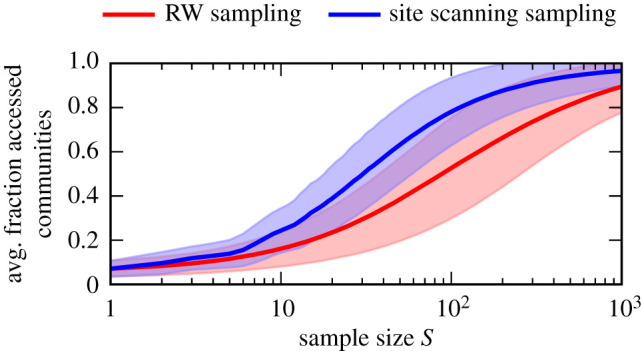
Average fraction of accessed communities as a function of the sample size S for random walk (RW) and site scanning sampling, averaged over the 200 largest NCs of the L = 12 RNA secondary structure GP map and 100 repetitions, respectively. The shaded bands indicate the standard deviation for the averaging over the 200 largest NCs. As the basis for the number of communities, respectively, we use the community structure with maximum modularity obtained by our sequence-based communities method. The results support the findings in figure 3b: site scanning sampling outperforms RW sampling in terms of a fast exploration of the NC communities.

In all the following sections, we employ site scanning sampling.

4. Community structure estimation

In a final step, we consider the NCs of longer, naturally occurring functional non-coding RNA sequences. Such RNA sequences can be found in the functional RNA database fRNAdb [30,31] (http://www.ncrna.org/ (accessed 3 October 2018)). Among other information, the fRNAdb also stores a prediction of the secondary structure. However, we only take the sequence from the fRNAdb and use the secondary structure predicted by the ViennaRNA package since our computational analysis relies on this package. The secondary structures stored in the fRNAdb and those predicted by the ViennaRNA package can differ.

An exhaustive analysis of the NC networks of such sequences is not feasible, and their community structure has to be estimated. In this section, we introduce a way to estimate the network of communities, i.e. the coarse-grained representation, of an NC from a sample of genotypes.

4.1. Methods

In order to create an approximate reconstruction of the network of NC communities from a genotype sample, we require estimates of three different types of information, as follows. Firstly, the list of constrained positions. Secondly, the realized letter combinations at these positions, which correspond to the communities. Thirdly, the relative frequency of the realized letter combinations.

In our original method, we found the optimal list of constrained positions by determining the average number of neutral mutations per site, and adding the positions of the constrained sites in order of their decreasing constraint to identify the community structure with maximum modularity. Here, this step-wise procedure is not feasible as it is not possible to calculate the modularity of certain community structures because the full NC is not known. In addition, longer RNA sequences exhibit a broader distribution of the average number of neutral mutations per site, which implies the possibility of multiple hierarchy layers. Thus, as a starting point, we use the paired sites for the constrained positions (as in [9]). Later, by inspecting the average number of neutral mutations per site and varying the threshold, we analyse the hierarchy layers.

We determine the average number of neutral mutations per site as follows. Starting from an fRNAdb sequence, we generate a sample of size S by using an accelerated version of the site scanning sampling, which was also introduced in [28]. Whereas site scanning sampling can be applied to any type of sequence, the accelerated version is an RNA-specific algorithm that reduces the computational costs in terms of the number of calls of the function RNA.fold. When a paired site is mutated, we only check the mutation for neutrality by calling RNA.fold if the mutated base pair is still one of the six RNA secondary structure compatible base pairs: CG, GC, AU, UA, GU and UG. Otherwise, we directly regard the mutation to be non-neutral and do not call RNA.fold. For the detailed algorithm of accelerated site scanning sampling, see the electronic supplementary material in [28]. Now, from the sample of size S, the average number of neutral mutations per site can be calculated by averaging over the sample genotypes. However, this requires the measurement of the one-point mutational neighbourhood of each sample genotype. This can be computationally expensive, in particular for longer RNA sequences. As suggested and tested in [28], a workaround is to consider a smaller random subsample of size S_r ≤ S from the sample of size S and to calculate the average number of neutral mutations per site only from these S_r genotypes. As done in [28], for the measurement of the one-point mutational neighbourhoods of the S_r subsample genotypes, we also use an RNA-specific updated version by employing the principle of only checking one-point mutations of paired sites for neutrality if the mutated base pair is still compatible. For the detailed algorithms of random subsampling and the one-point mutational neighbourhood measurement, see the electronic supplementary material in [28]. In a similar way, a restriction to compatible base pairs has been used in an algorithm by Jörg et al. [32] to estimate RNA neutral network sizes and robustness.

In order to estimate the set of letter combinations that can appear at the constrained positions, we record all letter combinations at the constrained positions across all available genotypes that we know to be part of the NC. On the one hand, these are the genotypes from the sample of size S. On the other hand, we check the neighbouring neutral genotypes that we find by measuring the one-point mutational neighbourhoods of the S_r random subsample genotypes. As we primarily consider the paired sites to be constrained, the average number of neutral mutations per site and therefore the one-point mutational neighbourhood measurement of the S_r random subsample genotypes is not necessary in the first place. However, as we will see later, including the neighbouring neutral genotypes of a random subsample will prove to be valuable in finding realized letter combinations and so coarse-grained communities.

From the relative frequency of the found letter combinations among the set of checked genotypes, we estimate the relative size of the associated coarse-grained communities.

Finally, bringing together all this information, we are able to make an estimate of the coarse-grained network representation in a similar way as for the short sequence lengths for which the full NC is known.

4.2. Results

The first example is an RNA sequence of length L = 20. It has the entry ID FR422569 in the fRNAdb and is an RNA found in Drosophila melanogaster. In figure 5, the community structure estimation results for its NC are shown. The figure also displays the predicted secondary structure in dot–bracket notation. This structure comprises six base pairs and slightly differs from the one given by the fRNAdb, which misses the outermost base pair.

Figure 5.

(a) Community structure estimation results for the NC comprising the fRNAdb sequence with entry ID FR422569 and length L = 20. For four sample and random subsample size combinations: (i) S = 1000, S_r = 100, (ii) S = 1000, S_r = S, (iii) S = 10 000, S_r = 100 and (iv) S = 10 000, S_r = S, the average number of neutral mutations per site averaged over the random subsample and the estimated coarse-grained network are shown. For the average number of neutral mutations per site, the shaded grey areas as well as the blue markers highlight the paired sites, i.e. the positions for which the realized letter combinations are associated with communities. For the coarse-grained network in (a(iv)), a force-directed graph layout is used, the networks in (a(i)), (a(ii)) and (a(iii)) are drawn with respect to this layout. (b) Coarse-grained network from (a(iv)) with coloured communities and (c) further coarse-grained networks according to the letter combinations at positions (i) ‘a’, (ii) ‘a’ and ‘b’, and (iii) ‘a’ and ‘c’ marked in (a(iv)), respectively. For the further coarse-grained networks, additionally, the associated letter combinations are shown. The results highlight that the coarse-grained network itself displays a community structure of which the most significant division is caused by the pair of most constrained paired sites (sites at positions ‘a’).

In figure 5a, for four sample and random subsample size combinations, the average number of neutral mutations per site and the force-directed layout of the estimated coarse-grained network are shown. While the average number of neutral mutations per site does not differ significantly for the four combinations, the coarse-grained network builds up with increasing sample and random subsample size. The maximum shown sample size and random subsample size is S = S_r = 10 000 (figure 5a(iv)), for which we find a coarse-grained network with a regular pattern. By using the NC size estimation formula introduced in [28], we estimate the NC size to be approximately 4.4 × 10⁶. By comparing it with the number of distinct genotypes that are checked for their letter combinations at the paired sites during this sampling and estimation process, we find that about 4% of the genotypes of the NC are covered.

The coarse-grained network itself displays a community structure, which can be explained by the distribution of the average number of neutral mutations per site. In figure 5a(iv), the two sites of the second outermost base pair are the most constrained. In figure 5b(i), the nodes of the respective coarse-grained network are coloured based on the letter combinations at these two positions, and in figure 5c(i), the related further coarse-grained network is shown. The results demonstrate that it is this pair of most constrained sites that is causing the most significant observable division of the coarse-grained network in the layout. The other paired sites have a more similar constraint. Within this group of sites, the two sites of the innermost base pair are the second most constrained ones. Figure 5b(ii) and c(ii) displays the coloured coarse-grained network and the further coarse-grained network, with respect to the letter combinations at the positions of the second outermost and the innermost base pair. While this additional base pair is definitely causing a division of the previously found communities into subcommunities, it is not causing the further division that is observable in the layout. As demonstrated with figure 5b(iii) and c(iii), it is the outermost base pair that is causing this observable further division. The likely reason is that the outermost and second outermost base pairs are adjacent to each other and therefore constrain the realizable letter combinations for stability reasons, such as the avoidance of adjacent wobble base pairs.

The second example is an RNA sequence of length L = 45. It has the entry ID FR039335 and is a hammerhead ribozyme (type I) found in Schistosoma mansoni. In figure 6, the community structure estimation results for its NC are shown. The predicted secondary structure differs from the one given by the fRNAdb. It has nine base pairs in two separate stem–loops, which is not the structure associated with a hammerhead ribozyme (type I). However, we will nevertheless use this example to illustrate how a coarse-grained network representation can be derived for a sequence of this length. It should also be noted that the secondary structure given by the fRNAdb would not be obtainable as a prediction from the ViennaRNA package. One of the stem–loops comprises no real loop, i.e. the base pair at the end of the stem spans no unpaired site, while ViennaRNA returns base pairs that always span at least three unpaired sites [23].

Figure 6.

(a) Community structure estimation results for the NC comprising the fRNAdb sequence with entry ID FR039335 and length L = 45. For four sample and random subsample size combinations: (i) S = 10 000, S_r = 100, (ii) S = 10 000, S_r = S, (iii) S = 100 000, S_r = 100 and (iv) S = 100 000, S_r = S, the average number of neutral mutations per site averaged over the random subsample and the estimated coarse-grained network are shown. For the average number of neutral mutations per site, the shaded grey areas as well as the blue markers highlight the paired sites, meaning the positions for which the realized letter combinations are associated with communities. For the coarse-grained network in (a(iv)), a force-directed graph layout is used, the networks in (a(i)), (a(ii)) and (a(iii)) are drawn with respect to this layout. (b) Coarse-grained networks ((i) for S = 10 000, S_r = S from (a(ii)) and (ii) for S = 100 000, S_r = S from (a(iv))) with coloured communities and (c) further coarse-grained networks according to the letter combinations at the positions marked by ‘α’ in (a(ii)) and (a(iv)). For the further coarse-grained networks, additionally, the associated letter combinations are shown. The results highlight that the most significant division of the coarse-grained network is caused by the more constrained paired sites in the left base pair stack of the secondary structure.

In figure 6a, again, for four sample and random subsample size combinations, the average number of neutral mutations per site and the force-directed layout of the estimated coarse-grained network are shown. As before, the average number of neutral mutations per site does not change significantly between the combinations, though the coarse-grained network builds up with increasing sample and random subsample size.

The coarse-grained network again reveals a community structure that can be explained with the average number of neutral mutations per site. The sites corresponding to the left stack of three base pairs are more constrained than those of the right base pair stack. In figure 6b and c, the coarse-grained network with coloured nodes according to the letter combinations at these positions and the related further coarse-grained network are shown for S = S_r = 10 000 and S = S_r = 100 000, respectively. The colouring matches the graph layouts of the coarse-grained networks, underlining that the stack of more constrained base pairs is causing the observable community division. For these three base pairs, for S = S_r = 10 000, we find 10 letter combinations and so communities, while for S = S_r = 100 000, we find four more letter combinations leading to a loop in the further coarse-grained network. This highlights that for this NC, and probably for longer RNA sequences in general, more letter combinations can be found for a three base pair stack than for the first and third example NC from figure 1 for L = 12.

For S = S_r = 100 000, only about 2.2 × 10⁻⁹% of the NC genotypes are covered (estimated NC size is approximately 2.4 × 10¹⁷ using [28]) in the respective sampling and estimation process. It raises the question of whether all realized letter combinations and coarse-grained communities are found. In figure 7,we plot the number of found communities as a function of the sample size for multiple random subsample sizes, respectively. In figure 7a, the hierarchy layer for considering all paired sites is examined. In this case, no saturation is observable over the considered range of sample sizes. Furthermore, using the full sample as the random subsample (S_r = S) leads to significantly more discovered communities than using the fixed smaller random subsample sizes of S_r = 100 and S_r = 1000. In figure 7b, the hierarchy layer for only considering the left base pair stack sites is examined. In this case, a saturation sets in with increasing sample size and there are fewer differences between the random subsample sizes. For all random subsample sizes, we find the 14 communities of this hierarchy layer for a sample size of S = 50 000.

Figure 7.

Number of found coarse-grained communities of the NC comprising the fRNAdb sequence with entry ID FR039335 and length L = 45 (also considered in figure 6) as a function of the sample size S for three random subsample sizes of S_r = 100, S_r = 1000 and S_r = S, respectively. (a) Hierarchy layer for considering all paired sites of the respective secondary structure and (b) hierarchy layer for only considering the more constrained left base pair (bp) stack sites. While there is no saturation for the former hierarchy layer, the number of found communities saturates for the latter hierarchy layer.

A potential workaround to find realized letter combinations faster could be as follows. Once an estimation with a given sample and random subsample size is completed, one could look at ‘open ends’ of the coarse-grained network, meaning coarse-grained nodes that are only connected to one other node (for example, see figure 6c(i)). By selecting a sequence from such a coarse-grained node, one could start a more specialized site scanning sampling process that still forces mutations of sites if possible but that does not allow mutations that would return to an existing coarse-grained node. This could lead to a faster discovery of unknown letter combinations and therefore of unknown coarse-grained nodes.

To summarize, the two examples show that, for longer RNA sequences, the consideration of the positions of the paired sites can already lead to coarse-grained network representations that themselves show a community structure if there are differences in the site constraints of the paired sites. In this case, similar to that seen for the initial sequence-based communities method, the community structure of the coarse-grained network is caused by the most constrained sites but now within all paired sites. It is probable that the longer the RNA sequence, the smaller the differences in the constraint of sites that can cause observable community divisions in the NC network.

We chose the two examples as the NCs display a particularly clear coarse-grained network representation with a further observable community division. We have also tested other fRNAdb sequences of similar lengths. For these sequences, either the paired sites were more similarly constrained (e.g. one continuous base pair stack)—such that the respective coarse-grained network representation did not show a further observable community division, caused by different site constraints along the paired sites—or the number of base pairs was larger, making the construction of the coarse-grained network computationally more expensive if all paired sites are included.

5. Discussion and conclusion

Building on previous work by Manrubia and co-workers [9,14], as well as by Greenbury [15], we introduced a method to reveal the hierarchical community structure of an NC, in the GP map of RNA secondary structure, solely from the sequence constraints and composition of the genotypes forming the NC. We identified the distribution of the average number of neutral mutations per site as the crucial starting point to identify different levels of constraint along the sequence positions. Using this knowledge, we showed that the hierarchical community layers can be revealed by proceeding through the positions in the order of their decreasing constraint and recording the realized letter combinations at these positions across the NC genotypes.

For the NCs of the L = 12 RNA secondary structure GP map, which are exhaustively known, we were able to find the most meaningful community structure in terms of the maximum modularity, respectively. For non-exhaustively known NCs formed by longer RNA sequences, a step-wise procedure to find the community structure with maximum modularity is not possible. Nonetheless, we outlined a way to estimate the coarse-grained community structure from a sample of genotypes. We found that observable community divisions can already be caused by differences in the constraints among the paired sites. To achieve meaningful estimates, quite large sample sizes have to be used to discover all or most of the realized letter combinations at the constrained positions. For example, for a base pair, there are three potential letter combinations within an NC. This means that the number of potential letter combinations just at the paired sites increases exponentially with the number of base pairs in the phenotype and so also with sequence length. Using accelerated site scanning sampling and additionally measuring the one-point mutational neighbourhoods of random subsample genotypes have been shown to improve the estimates.

Our introduced methods improve the understanding of the community structure of NCs. The community structure of NCs is likely to have an impact on evolutionary processes, as has been demonstrated for other topological properties of NCs previously [18–20]. Here, we showed that a RW (which is quite similar to an evolutionary process) on an NC dominantly proceeds within rather than between individual communities as the connections between communities can be seen as ‘bottlenecks’. This implies that from all alternative phenotypes surrounding an NC, which is sometimes referred to as the NC evolvability, only those surrounding the community of the starting genotype are likely to be reachable by evolution without leaving the NC, if the NC exhibits a pronounced community structure. In the future, more research should be done on the impact of the NC community structure.

We applied the framework to the NCs of the GP map of RNA secondary structure. However, the framework is not GP map specific and can almost certainly be transferred to many other GP maps. For other GP maps, the distribution of the average number of neutral mutations per site might be less bimodal than for RNA secondary structure for which paired sites are mostly constrained and unpaired sites are mostly unconstrained. Nevertheless, a similar approach to the one presented here, based on a step-wise consideration of decreasing sequence constraint, is likely to be successful in other GP maps, too.

Other GP maps this framework could be applied to include those of the HP lattice model [33–35] or the Polyomino model [12,16], which describe different levels of protein structure. For the latter model, owing to the more symmetric mapping between genotypes and phenotypes compared with RNA secondary structure, the community structures might be even more symmetric or pronounced than in RNA, as preliminary work by Greenbury has shown [15]. A more ambitious aim would be to apply this approach to more complex biological GP maps, such as protein secondary structure and protein tertiary structure, which are so large that sampling approaches are absolutely essential. Lastly, the approach could be applied to empirical GP maps like the one of transcription factor binding sites [17]. For this GP map, the community structure of genotype networks has been studied previously [17]. Using our sequence-based method might reveal a relationship between the communities and dual modes of binding specificity or other features of the interactions between transcription factors and binding sites [17,36].

Data accessibility

The code to generate the data shown in this article and the data itself can be accessed at: https://github.com/mw636/NC-community.git.

Authors' contributions

M.W. and S.E.A. designed the analysis, M.W. carried out the analysis, M.W. and S.E.A. wrote the manuscript.

Competing interests

We declare we have no competing interests.

Funding

M.W. was supported by the EPSRC and the Gatsby Charitable Foundation. S.E.A. was supported by the Gatsby Charitable Foundation and the Alan Turing Institute.

References

- 1.Wright S. 1932. The roles of mutation, inbreeding, crossbreeding, and selection in evolution. Proc. Sixth Int. Congr. Genet. 1, 355–366. [Google Scholar]
- 2.Maynard Smith J. 1970. Natural selection and the concept of a protein space. Nature 225, 563–564. ( 10.1038/225563a0) [DOI] [PubMed] [Google Scholar]
- 3.Eigen M, Winkler-Oswatitsch R, Dress A. 1988. Statistical geometry in sequence space: a method of quantitative comparative sequence analysis. Proc. Natl Acad. Sci. USA 85, 5913–5917. ( 10.1073/pnas.85.16.5913) [DOI] [PMC free article] [PubMed] [Google Scholar]
- 4.Greenbury SF, Schaper S, Ahnert SE, Louis AA. 2016. Genetic correlations greatly increase mutational robustness and can both reduce and enhance evolvability. PLoS Comput. Biol. 12, 1–27. ( 10.1371/journal.pcbi.1004773) [DOI] [PMC free article] [PubMed] [Google Scholar]
- 5.Schuster P, Fontana W, Stadler PF, Hofacker IL. 1994. From sequences to shapes and back: a case study in RNA secondary structures. Proc. R. Soc. Lond. B 255, 279–284. ( 10.1098/rspb.1994.0040) [DOI] [PubMed] [Google Scholar]
- 6.Schuster P. 1995. How to search for RNA structures Theoretical concepts in evolutionary biotechnology. J. Biotechnol. 41, 239–257. ( 10.1016/0168-1656(94)00085-Q) [DOI] [PubMed] [Google Scholar]
- 7.Fontana W. 2002. Modelling ‘evo-devo’ with RNA. BioEssays 24, 1164–1177. ( 10.1002/bies.10190) [DOI] [PubMed] [Google Scholar]
- 8.Wagner A. 2008. Robustness and evolvability: a paradox resolved. Proc. R. Soc. B 275, 91–100. ( 10.1098/rspb.2007.1137) [DOI] [PMC free article] [PubMed] [Google Scholar]
- 9.Aguirre J, Buldú JM, Stich M, Manrubia SC. 2011. Topological structure of the space of phenotypes: the case of RNA neutral networks. PLoS ONE 6, 1–15. ( 10.1371/annotation/b3e79f42-7316-4ff8-9762-514120463813) [DOI] [PMC free article] [PubMed] [Google Scholar]
- 10.Ferrada E, Wagner A. 2012. A comparison of genotype-phenotype maps for RNA and proteins. Biophys. J. 102, 1916–1925. ( 10.1016/j.bpj.2012.01.047) [DOI] [PMC free article] [PubMed] [Google Scholar]
- 11.Schaper S, Johnston IG, Louis AA. 2012. Epistasis can lead to fragmented neutral spaces and contingency in evolution. Proc. R. Soc. B 279, 1777–1783. ( 10.1098/rspb.2011.2183) [DOI] [PMC free article] [PubMed] [Google Scholar]
- 12.Greenbury SF, Johnston IG, Louis AA, Ahnert SE. 2014. A tractable genotype-phenotype map modelling the self-assembly of protein quaternary structure. J. R. Soc. Interface 11, 20140249 ( 10.1098/rsif.2014.0249) [DOI] [PMC free article] [PubMed] [Google Scholar]
- 13.Dingle K, Schaper S, Louis AA. 2015. The structure of the genotype–phenotype map strongly constrains the evolution of non-coding RNA. Interface Focus 5, 20150053 ( 10.1098/rsfs.2015.0053) [DOI] [PMC free article] [PubMed] [Google Scholar]
- 14.Capitán JA, Aguirre J, Manrubia S. 2015. Dynamical community structure of populations evolving on genotype networks. Chaos Solitons Fractals 72, 99–106. ( 10.1016/j.chaos.2014.11.019) [DOI] [Google Scholar]
- 15.Greenbury SF. 2014. General properties of genotype–phenotype maps for biological self-assembly. PhD thesis, University of Cambridge, Cambridge, UK. [Google Scholar]
- 16.Johnston IG, Ahnert SE, Doye JPK, Louis AA. 2011. Evolutionary dynamics in a simple model of self-assembly. Phys. Rev. E 83, 066105 ( 10.1103/PhysRevE.83.066105) [DOI] [PubMed] [Google Scholar]
- 17.Aguilar-Rodríguez J, Peel L, Stella M, Wagner A, Payne JL. 2018. The architecture of an empirical genotype-phenotype map. Evolution 72, 1242–1260. ( 10.1111/evo.13487) [DOI] [PMC free article] [PubMed] [Google Scholar]
- 18.van Nimwegen E, Crutchfield JP, Huynen M. 1999. Neutral evolution of mutational robustness. Proc. Natl Acad. Sci. USA 96, 9716–9720. ( 10.1073/pnas.96.17.9716) [DOI] [PMC free article] [PubMed] [Google Scholar]
- 19.Manrubia S, Cuesta JA. 2015. Evolution on neutral networks accelerates the ticking rate of the molecular clock. J. R. Soc. Interface 12, 20141010 ( 10.1098/rsif.2014.1010) [DOI] [PMC free article] [PubMed] [Google Scholar]
- 20.Aguirre J, Catalán P, Cuesta JA, Manrubia S. 2018. On the networked architecture of genotype spaces and its critical effects on molecular evolution. Open Biol. 8, 180069 ( 10.1098/rsob.180069) [DOI] [PMC free article] [PubMed] [Google Scholar]
- 21.Hofacker IL, Fontana W, Stadler PF, Bonhoeffer LS, Tacker M, Schuster P. 1994. Fast folding and comparison of RNA secondary structures. Monatshefte für Chemie/Chem. Mon. 125, 167–188. ( 10.1007/BF00818163) [DOI] [Google Scholar]
- 22.Hofacker IL. 2003. Vienna RNA secondary structure server. Nucleic Acids Res. 31, 3429–3431. ( 10.1093/nar/gkg599) [DOI] [PMC free article] [PubMed] [Google Scholar]
- 23.Lorenz R, Bernhart SH, Zu Siederdissen CH, Tafer H, Flamm C, Stadler PF, Hofacker IL. 2011. ViennaRNA Package 2.0. Algorithms Mol. Biol. 6, 26 ( 10.1186/1748-7188-6-26) [DOI] [PMC free article] [PubMed] [Google Scholar]
- 24.Newman MEJ, Girvan M. 2004. Finding and evaluating community structure in networks. Phys. Rev. E 69, 026113 ( 10.1103/PhysRevE.69.026113) [DOI] [PubMed] [Google Scholar]
- 25.Newman MEJ. 2004. Fast algorithm for detecting community structure in networks. Phys. Rev. E 69, 066133 ( 10.1103/PhysRevE.69.066133) [DOI] [PubMed] [Google Scholar]
- 26.Blondel VD, Guillaume JL, Lambiotte R, Lefebvre E. 2008. Fast unfolding of communities in large networks. J. Stat. Mech: Theory Exp. 2008, P10008 ( 10.1088/1742-5468/2008/10/P10008) [DOI] [Google Scholar]
- 27.Reichardt J, Bornholdt S. 2006. Statistical mechanics of community detection. Phys. Rev. E 74, 016110 ( 10.1103/PhysRevE.74.016110) [DOI] [PubMed] [Google Scholar]
- 28.Weiß M, Ahnert SE. 2020. Using small samples to estimate neutral component size and robustness in the genotype–phenotype map of RNA secondary structure. J. R. Soc. Interface 17, 20190784 ( 10.1098/rsif.2019.0784) [DOI] [PMC free article] [PubMed] [Google Scholar]
- 29.Masuda N, Porter MA, Lambiotte R. 2017. Random walks and diffusion on networks. Phys. Rep. 716–717, 1–58. ( 10.1016/j.physrep.2017.07.007) [DOI] [Google Scholar]
- 30.Kin T. et al 2007. fRNAdb: a platform for mining/annotating functional RNA candidates from non-coding RNA sequences. Nucleic Acids Res. 35, D145–D148. ( 10.1093/nar/gkl837) [DOI] [PMC free article] [PubMed] [Google Scholar]
- 31.Mituyama T, Yamada K, Hattori E, Okida H, Ono Y, Terai G, Yoshizawa A, Komori T, Asai K. 2008. The functional RNA Database 3.0: databases to support mining and annotation of functional RNAs. Nucleic Acids Res. 37, D89–D92. ( 10.1093/nar/gkn805) [DOI] [PMC free article] [PubMed] [Google Scholar]
- 32.Jörg T, Martin OC, Wagner A. 2008. Neutral network sizes of biological RNA molecules can be computed and are not atypically small. BMC Bioinf. 9, 464 ( 10.1186/1471-2105-9-464) [DOI] [PMC free article] [PubMed] [Google Scholar]
- 33.Lau KF, Dill KA. 1989. A lattice statistical mechanics model of the conformational and sequence spaces of proteins. Macromolecules 22, 3986–3997. ( 10.1021/ma00200a030) [DOI] [Google Scholar]
- 34.Lipman DJ, Wilbur WJ, Smith JM. 1991. Modelling neutral and selective evolution of protein folding. Proc. R. Soc. Lond. B 245, 7–11. ( 10.1098/rspb.1991.0081) [DOI] [PubMed] [Google Scholar]
- 35.Li H, Helling R, Tang C, Wingreen N. 1996. Emergence of preferred structures in a simple model of protein folding. Science 273, 666–669. ( 10.1126/science.273.5275.666) [DOI] [PubMed] [Google Scholar]
- 36.Badis G. et al. 2009. Diversity and complexity in DNA recognition by transcription factors. Science 324, 1720–1723. ( 10.1126/science.1162327) [DOI] [PMC free article] [PubMed] [Google Scholar]
Associated Data
This section collects any data citations, data availability statements, or supplementary materials included in this article.
Data Availability Statement