Abstract
Joint models for longitudinal biomarkers and time-to-event data are widely used in longitudinal studies. Many joint modeling approaches have been proposed to handle different types of longitudinal biomarkers and survival outcomes. However, most existing joint modeling methods cannot deal with a large number of longitudinal biomarkers simultaneously, such as the longitudinally collected gene expression profiles. In this article, we propose a new joint modeling method under the Bayesian framework, which is able to analyze longitudinal biomarkers of high dimension. Specifically, we assume that only a few unobserved latent variables are related to the survival outcome and the latent variables are inferred using a factor analysis model, which greatly reduces the dimensionality of the biomarkers and also accounts for the high correlations among the biomarkers. Through extensive simulation studies, we show that our proposed method has improved prediction accuracy over other joint modeling methods. We illustrate the usefulness of our method on a dataset of idiopathic pulmonary fibrosis patients in which we are interested in predicting the patients’ time-to-death using their gene expression profiles.
Keywords: Bayesian factor analysis, Joint models, Longitudinal biomarkers of high dimension, Survival prediction
1. Introduction
In longitudinal studies, it is often of great interest to study the association between a biomarker repeatedly measured over time and the survival outcome. Many methods have been proposed to assess this association, such as the landmarking methods (Anderson et al., 1983; van Houwelingen and Putter, 2011) and the joint modeling methods (Faucett and Thomas, 1996; Tsiatis and Davidian, 2004; Rizopoulos et al., 2014). Among these approaches, joint modeling methods of longitudinal and time-to-event data have been widely used, because they are able to model the longitudinal biomarker as well as the survival time flexibly and appropriately and they can provide individualized dynamic predictions based on all past values of the longitudinal biomarker (Rizopoulos et al., 2014).
In our motivating study, a cohort of patients with idiopathic pulmonary fibrosis (IPF) were followed longitudinally (Herazo-Maya et al., 2013). IPF is a highly lethal lung disease with median survival time being three to five years after diagnosis. At each visit, gene expression profiles in the peripheral blood mononuclear cells were measured for the patients. The time-to-event and important clinical variables were recorded for these patients as well. Here, we are interested in predicting the patients’ survival time using relevant clinical variables and the repeatedly measured gene expression profiles, where the joint modeling approach serves as a promising tool.
During the last two decades, many joint modeling methods have been proposed to deal with different types of longitudinal biomarkers and survival outcomes. (Tsiatis and Davidian, 2004) provided a comprehensive overview of some early work on joint models and (Proust-Lima et al., 2014) discussed some recent advances on this topic. For instance, (Brown et al., 2005) proposed a joint modelling method in which cubic B-splines were introduced to model the longitudinal markers flexibly and their approach can deal with multivariate biomarkers, but is limited to only a few of them. In order to further increase the flexibility of the longitudinal submodel, (Rizopoulos and Ghosh, 2011) developed a spline-based approach for longitudinal outcomes with unusual time-dependent shapes. To improve the computation efficiency, (Rizopoulos, 2012) proposed to use a pseudo-adaptive Gauss-Hermite quadrature rule to achieve a fast computation for integrations in joint models, which are usually computationally intensive to calculate, especially when the number of random effects is large. (Rizopoulos et al., 2014) used the Bayesian model averaging idea in the joint modeling framework to obtain individualized prediction by aggregating results from different types of submodels. (He et al., 2015) developed a penalized likelihood method with LASSO penalty for simultaneous selection of fixed and random effects in joint models. However, all aforementioned methods cannot deal with a large number of biomarkers simultaneously, such as the gene expression profiles in our study. The number of subject-specific random effects and the dimension of the covariance matrix of the random effects for all biomarkers grow rapidly as the number of biomarkers increases, which makes those methods computationally intractable.
In this article, we propose a new joint modeling method under the Bayesian framework to deal with longitudinal biomarkers of high dimension. Specifically, we assume that only a few unobserved latent variables are related to the survival outcome. We adopt a factor analysis model (West, 2003; Carvalho et al., 2008) to infer the latent variables, which greatly reduces the dimensionality of the biomarkers. In addition, the factor analysis model can also account for the high correlations among the biomarkers, as often observed in the gene expression data. The factor analysis model is integrated into the joint modeling framework so that the uncertainties in the inference of the latent variables can be appropriately accounted for when making predictions.
The remainder of the article is organized as follows. Section 2 describes our proposed model. Section 3 presents our estimation procedure and survival prediction method. Section 4 shows the performance of our proposed method in simulation studies. Section 5 illustrates the application of our proposed model on the IPF dataset. Section 6 concludes the article with some remarks.
2. Model specification
2.1. Longitudinal submodel
Let denote the gene expression profiles for subject i at time point t, where G is the total number of genes. Then a standard factor analysis model can be written as:
| (1) |
where is a K-dimensional latent factor score vector for the ith subject at time point t with K being some pre-specified number of factors (see Section 3 for details in choosing K), Λ is a G × K factor loading matrix, ε(i)(t) are measurement errors of the gene expression profile for subject i at time point t, and are the gene-specific variances for the measurement errors.
As in most joint modeling methods, we adopt linear mixed-effects models for the factor scores η(i)(t) as follows. For k = 1,2, ⋯, K,
| (2) |
where βk are the fixed effects, are the centered random effects specific for subject i with Dk being the covariance matrix for the random effects in the kth factor scores, and denote the time-dependent design vectors for subject i. In general, any covariates of interest and any functions of t can be specified in and .
Constraints have to be placed on the factor loading matrix Λ to ensure identifiability. As commonly done, we constrain Λ to be a lower-triangular matrix with all diagonal elements being one so that we can model the factor scores flexibly (Erosheva and Curtis, 2011). In the Bayesian framework, we can easily integrate the factor analysis model into the joint modeling framework and fit them simultaneously. Specifically, only the η(i)(t) enter into the survival submodel and hence the dimension of the biomarkers can be largely reduced, since the number of factors K ≪ G in practice.
2.2. Survival submodel
Denote the observed event time for subject i by Ti, the minimum of the censoring time Ci and the true event time . Let denote the event indicator for subject i, where I(·) is the indicator function taking value 1 if and 0 otherwise.
We assume that the association between the gene expression profiles and the survival outcome is induced by the latent variables and hence only the factor scores η(i)(t) enter into the survival submodel. To be specific, we take the form of hazard function as
| (3) |
where denotes the history of the unobserved longitudinal latent process up to time t for subject i, ωi denotes the baseline covariates for subject i with corresponding regression coefficients γ, the parameters in α quantify the associations between the latent factor scores and the survival outcome, and h0(·) is the baseline hazard function. To specify the survival process, h0(·) is assumed to be a piecewise constant function to allow for flexibility, as done in (Taylor et al., 2013), that is
| (4) |
where {Bq: q = 1, ⋯, Q+1} are the pre-specified knots with corresponding function values {ρq: q = 1, ⋯, Q} on each interval. Selection of knots in h0(·) is crucial because too many knots may lead to overfitting while too few knots make the model less flexible. In our work, we fix B1 = 0 and BQ+1 = ∞ and choose the positions of other knots as the Q-quantiles of the observed event times to ensure similar numbers of events in each interval, as commonly done (Taylor et al., 2013; Rizopoulos et al., 2014).
3. Estimation and prediction
3.1. Simultaneous estimation of submodels
We perform Markov chain Monte Carlo algorithm (MCMC) to estimate parameters in the submodels jointly. Following previous work (Taylor et al., 2013; Rizopoulos et al., 2014), we assume that longitudinal outcomes and the survival process are independent conditional on the random effects. Meanwhile, latent factors of each subject are assumed to be independent. Let and we have
| (5) |
where ni is the number of repeated measures for subject i and denotes all parameters with θt denoting the parameters in the survival process, θe the parameters in the factor scores, θy the parameters in the factor analysis model, and θb the covariance matrices of the random effects. The posterior distribution of the random effects b(i) and parameters θ conditional on the observed data can be written out as
| (6) |
Under the assumption that censoring mechanism and the visiting time are independent of the true event time given the observed history, we can derive the likelihood contribution for subject i conditional on θ and b(i) by substituting the latent factor η(i)(t), that is
| (7) |
where β = (β1, β2, ⋯, βK)T and denotes the gth row of the loading matrix Λ.
The number of factors K is usually unknown in practice. Here, we adopt the deviance information criterion (DIC) (Gelman et al., 2014) to select the number of factors based on the full likelihood derived from Equation (7) (See Section 4 for the performance). DIC is a criterion for model comparison based on the balance between model fit and model complexity, both of which depend on the number of factors selected in the model. Also, it is worth noting that both the number of factors and the loading matrix depend on the longitudinal and survival submodels. In fact, the survival submodel tends to make the factor scores as predictive as possible while the longitudinal submodel favors the factor scores that explain a large proportion of the variations in the biomarkers. In this sense, our proposed model has similar flavor to the partial least squares regression (Geladi and Kowalski, 1986).
When nonlinear functions of t exist in x(i)(t) or z(i)(t), the integral in (7) does not have a closed-form solution, in which case a numerical method must be employed for its evaluation. A favorable choice for this calculation is a 15-point Gauss-Kronrod quadrature rule (Press, 2007). In this paper, x(i)(t) and z(i)(t) are both set to include only linear functions of t for two reasons. One reason is that most of the longitudinal biomarkers in our IPF dataset seem to have a linear trend over time (See Figure 1). The other reason is that extra non-linear terms will probably cause overfitting because the number of time points per patient is about three or four in our dataset. In fact, extension to nonlinear functions is easy to implement in practice using the Gauss-Kronrod quadrature rule.
Fig. 1.
Subject-specific gene expression trends over time for two selected genes TMEM170 and DMRTA1 in the IPF dataset.
We choose conjugate prior distributions for most parameters in our model to facilitate computation. In particular, for the fixed effects β in the longitudinal submodel and coefficients α and γ in the survival submodel, we pick independent diffuse normal priors. The standard normal prior distribution is specified for each free element in the factor loading matrix Λ. We choose independent Gamma distributions for the reciprocal of the gene-specific variances, and the parameters (ρ1, ρ2, ⋯, ρQ) in the baseline hazard function h0(·). Finally, independent InverseWishart distributions are specified to be the prior distributions for (D1, D2, ⋯, DK), the covariance matrices for the random effects. More details on the MCMC implementation are given in Appendix A of the Supplementary Materials.
3.2. Dynamic prediction
The primary goal of the joint modeling methods is to predict the event time for each subject based on his/her past observations and update the prediction dynamically when new observations are available. In our proposed method, it is straightforward to predict the subject-specific event time for a new subject j given this subject’s longitudinal biomarkers recorded up to any time point t. Let denote the longitudinal biomarkers from subject j recorded up to time point t, which also implies that this subject’s true event time For any u > t, the probability that subject j will survive at least up to u can be written as
| (8) |
Where are the observed longitudinal biomarkers and survival outcomes in training data and ωj are the baseline covariates of subject j. Let b(j) denote the random effects for subject j. According to (Taylor et al., 2013) and (Rizopoulos et al., 2014), we have
| (9) |
where S(·|θ,b(j)) is the survival function defined as:
| (10) |
With the posterior samples of the parameters θ obtained using the training data , a straightforward MCMC procedure can be implemented to sample b(j) from its posterior distribution given . Based on the posterior samples of θ and b(j), we can obtain the prediction of ζj(u|t) via Monte Carlo simulation. Detailed prediction algorithm for ζj(u|t) is provided in Appendix B of the Supplementary Materials.
4. Simulation studies
4.1. Simulation setting
In this section, we study the prediction performance of our proposed method through simulation studies. We also assess the performance of using DIC to choose the number of factors.
To mimic our IPF dataset, the number of subjects is 50, the number of genes is 50, the number of visits per subject is randomly drawn from {2,3,4,5} with equal probability, and the time points for each subject are randomly drawn from Uniform(0,1) in addition to the baseline visit. There are two baseline covariates (ωi) in our simulation, which are generated using . Also, there are three factors (K = 3) in our simulation and the corresponding factor scores η(i)(t) for subject i are generated as where and .
The survival time for each subject is generated based on the hazard function in Equation (3) with all parameters of the covariate effects (γ and α) being 1 and the baseline hazard function h0(t) being the hazard function of the Weibull(15,3) distribution. The censoring time Ci is independently drawn from Weibull(3,3) distribution so that the censoring rate is about 35%. The gene expression profiles are generated using Equation (1), where both the nonzero free elements in loading matrix Λ and the errors are independently generated from . In particular, a sparse loading matrix Λ is used, where the 4th to 20th, 21st to 35th, and 36th to 50th free elements of the first, second, and third factors are nonzero, respectively. We think this data generating process is comprehensive enough to mimic a gene correlation structure that is complicated enough as one would usually observe in real applications. First, the correlation matrix of the genes varies with time point t and the individual level random effect b(i). Second, since the loading matrix Λ is set to be sparse, the genes are naturally divided into three distinctive groups that correlation across different groups are 0. Finally, within each group, correlation between each pair of genes usually locates on (−0.5, 0.5), representing either strong or weak and positive or negative correlations of the genes.
In total, we simulate 200 datasets. In each dataset, we generate a set of testing data having 30 subjects, which is used to assess the predictive performance. In the training process, we choose (nearly) non-informative priors for our parameters to make the posterior nearly not affected by hyperparameters of the prior. More specifically, we choose the standard normal distribution for the prior distribution for each of the free elements in the factor loading matrix Λ (Ghosh and Dunson, 2009), Q = 4 for the number of knots in the baseline hazard funciton, Gamma(0.1, 0.1) for the distribution of (ρ1, ρ2, ρ3, ρ4) in the baseline hazard function, for the covariate effects of parameters (β, α, γ), and InverseWishart(I2×2, 3) for the distribution of the covariance matrices of the random effects (D1, D2, ⋯, DK), and Gamma(0.01,0.01) distribution for the reciprocal of the gene-specific variances . We run our model with a given number of factors on each dataset for 150,000 iterations with the first 70,000 samples discarded as burn-ins. By visually inspecting the trace plots of all parameters and examining their Geweke score (Geweke et al., 1991), there is no significant evidence of convergence issues. Examples of the convergence diagnostic for MCMC are provided in Appendix C of the supplement material.
4.2. Estimation in the Factor Analysis Model
The number of factors and the estimation of the loading matrix in the factor analysis are two important aspects of the factor analysis model, since the former one is related to the prediction performance while the latter one allows us to identify the driving biomarkers in each factor and gain insights on the biological mechanisms involved in the disease.
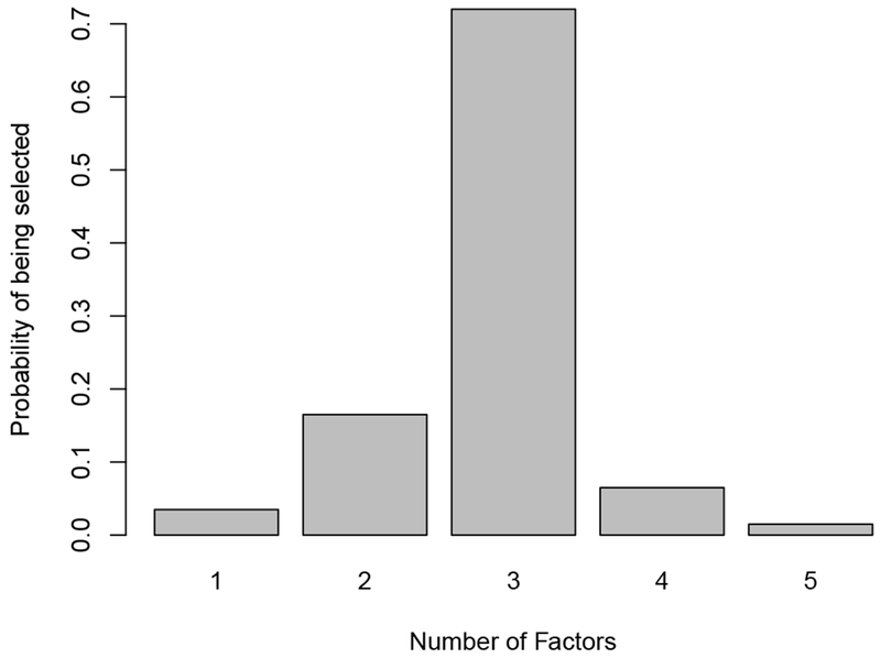
To evaluate how well DIC performs in selecting the number of factors K, we calculate the DICs for all models with the number of factors varying from 1 to 5. For each simulation dataset, the proportion of factors with the smallest DIC value is recorded. The true number of factors in the simulation datasets is 3 and the distribution of the number of factors being selected is shown in Figure 2. In 72% of the 200 experiments, the model with 3 factors has the smallest DIC. Also, in 95% of the 200 experiments, the number of factors being selected is among 2, 3 and 4, which is close to the true value. Therefore, our simulation results suggest that DIC performs well in selecting the number of factors. In addition, it is interesting to see if the nonzero free elements (i.e. the driving biomarker) in each factor can be correctly selected. Since we do not add sparsity on the loading matrix in our model, we calculate the Spearman’s rank correlation coefficients between the estimated loading matrix and the true loading matrix. The mean and standard deviation for the averages of the absolute values of the rank correlation coefficients over three factors is 0.72 and 0.06 based on the 200 datasets, respectively, suggesting that our model performs reasonably well in selecting the driving biomarkers in each factor.
Fig. 2.
The distribution of the numbers of factors selected by DIC on the 200 simulated datasets.
4.3. Assessment of Predictive Performance
To evaluate the predictive performance of our proposed model, we design two other models for comparison. For the first model, we pick the biomarker with the largest factor in the kth column of the true factor loading matrix Λ for k = 1, 2, 3 respectively. Since the true Λ has a group structure, we can exactly pick three biomarkers in this way and use them as the longitudinal covariates to fit a standard joint model. With our knowledge about the true model, this procedure is actually biased to favor of this benchmark method and selecting the most three informative biomarkers to construct the benchmark model. This model is denoted as JMsig and will be the first choice of the researchers when the dimension of longitudinal covariates is high and the standard joint models fail. For the second model, we first select three biomarkers at random and then a standard joint model is fitted with these randomly selected genes as in the first model. We refer to this model as JMran. Note that the number of biomarkers selected for these two benchmark models is equal to the true number of factors. And we refer to our proposed model as FAJM (Factor Analysis Joint Model) in comparisons with the two benchmarks.
To measure the predictive performance, we adopt the AUC approach for joint models proposed in (Rizopoulos et al., 2014). Suppose that there is a randomly chosen pair of patients {i, j} and both of them are event-free up to time t. Using their longitudinal measurements up to t, we can estimate ζi(u|t) and ζj(u|t) for any given u > t via our prediction procedure. Then, the area under curve (AUC) is defined as
| (11) |
where and are true event time of i and j. If subject j experiences event within (t, u] while subject i is event-free during this period, joint models with good prediction performance are expected to assign to subject i the higher probability for surviving longer than u, which is equivalent to ζi(u|t) > ζj(u|t). In practice, selection of a relevant time point u is crucial for clinical decision.
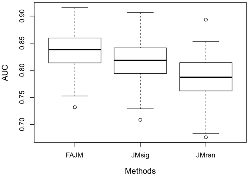
We calculate the AUCs for the three models for each of the 200 simulated datasets. Specifically, for each pair {i, j} considered in the testing data with , we take proper values of t and u to ensure and . Then, we can estimate the AUC by counting the percentage of such {i, j} that satisfies ζi(u|t) > ζj(u|t). Figure 3 shows the boxplots of the estimated AUCs for FAJM, JMsig, and JMran on the 200 simulated datasets, suggesting that FAJM has improved prediction compared to the other two models and that including only the most significant biomarkers in the model might not be the optimal choice in terms of prediction.
Fig. 3.
Boxplots of the estimated AUCs for FAJM, JMsig, and JMran on the 200 simulated datasets.
4.4. Sensitivity of the Results
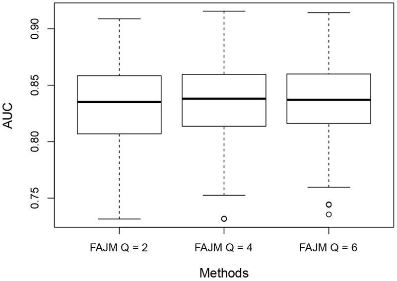
It is of our interests to investigate the influence of our choice of some hyperparameters for the model on statistical inference. In this section, we present our sensitivity analysis through simulation studies. First, we study the impact of the choice of Q(= 4), i.e. the number of distinctive intervals in the baseline hazard function h0 (·). Although one would expect the choice of Q is important to the joint model’s performance in risk prediction, it was suggested in the literature (Taylor et al., 2013) that the model is usually not sensitive to the numbers and positions of these knots when they are chosen within a proper scale. To study this issue, we conduct simulation studies with Q chosen as 2 and 6. Again, the knots are selected as the empirical Q-quantiles of the event time and other simulation settings remain the same. The resulting AUC values are compared across Q = 2, 4, 6 in Figure 4. It can be seen that the resulting AUCs are very close for different choices of Q so the performance of our method is not sensitive to the choice of Q when it varies within a certain range.
Fig. 4.
Boxplots of the estimated AUCs for FAJM with Q, the number of intervals in the baseline hazard set to be 2, 4 and 6, respectively on the 200 simulated datasets.
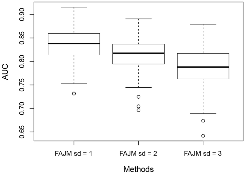
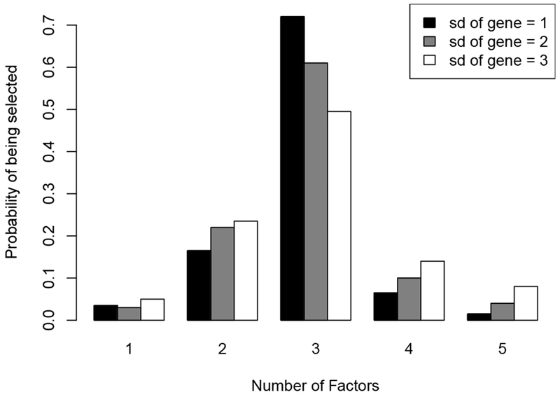
Second, we note that the amount of the survival information carried by the high dimensional biomarkers is determined by the signal-to-noise ratio (SNR) of the factor analysis model. When the variance of the noise for each biomarker increases, the SNR will decrease and the biomarkers will become less informative to the survival outcome. To study the impact of SNR, we conduct simulation studies where the variance of is increased from 1 to 4 and 9. We compare the estimation performance in the factor analysis model and the predictive performance for the survival outcome of our methods across different settings for the magnitude of the noise. The number of factors being selected for each setting is shown in Figure 5 and the resulting AUCs are presented in Figure 6. As the noise variance grows, both the predictive accuracy and the factorization performance of the FAJM decreases moderately.
Fig. 5.
Boxplots of the estimated AUCs for FAJM with the standard deviation (sd) of the gene’s noise set to be 1, 2 and 3, respectively on the 200 simulated datasets.
Fig. 6.
The distribution of the numbers of factors selected by DIC on the 200 simulated datasets, with the sd of set to be 1, 2 and 3
5. Application to the IPF dataset
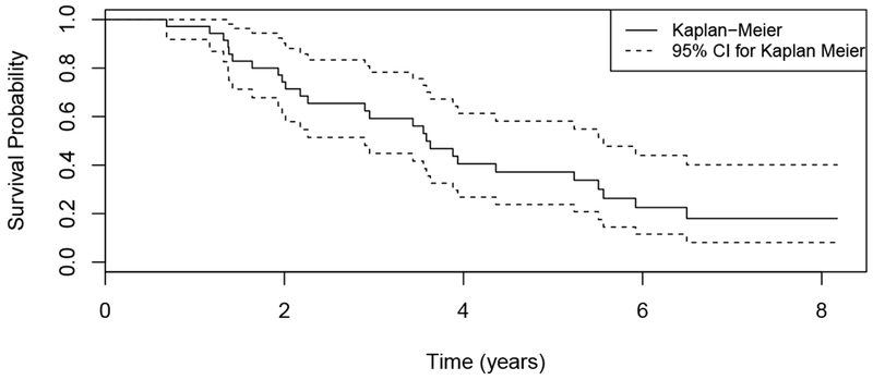
In this section, we apply our proposed method to the IPF dataset that was briefly described in Section 1. IPF is a highly lethal lung disease with the only effective intervention being lung transplantation. However, due to the limited availability of lung donors, it is important to prioritize the patients based on their risks to receive transplantation. In the current clinical setting, the GAP score is widely used as an indicator of disease stage for IPF patients, which is calculated based on the patient’s clinical information, including gender (G), age (A) and two lung physiology variables (P) (Ley et al., 2012). A higher GAP score indicates higher risk of death. In the IPF dataset, there are a total of 26 patients with the median number of visits being 3 (see Figure 1), the number of deaths being 17 and the number of censoring being 9. We include 55 genes in this analysis, which are related to the survival outcomes for IPF patients in an independent dataset. The Kaplan-Meier estimate of the survival function is shown in Figure 7, where we can see that the median survival time is about four years. Our goal is to build a risk prediction model using the baseline GAP scores and the longitudinal biomarkers to assess whether the longitudinal biomarkers are significantly associated with the survival outcome and hence could potentially be used to improve prediction in the clinical setting.
Fig. 7.
Kaplan-Meier plot (with 95% CI) of the time-to-event for the 26 patients in the IPF dataset.
The survival submodel in the IPF dataset is specified as
| (12) |
where h0(t) is assumed to be constant over four intervals whose knots are chosen to be (B1, B2, B3, B4, B5) = (0, 2, 3.6, 5.6, ∞) years. The hyperparameters in the prior distributions are chosen to be the same as our simulation studies, which was described in Section 4. We run our model with the number of factors K varying from 1 to 5 and we run a single chain of 200,000 MCMC iterations for each K. The first 100,000 iterations are discarded as burn-in and we find no evidence for poor convergence based on their trace plots and Geweke score (Geweke et al., 1991) of all parameters. Again, the diagnostics for MCMC convergence are presented in the supplement materials. In addition, we include sensitivity analysis to demonstrate that our prior is non-informative, e.g., having negligible effect on the results and present it in Figure S3 of the supplement material. The DIC values for the models with the number of factors being K = 1, 2, 3, 4, 5 are 2516.30, 2379.90, 2292.32, 2367.09, and 2767.81, respectively, which suggests the model with K = 3 fits the data best and hence we focus this model in the following discussion. The estimates (with 95% credible intervals) for γ1, α1, α2 and α3 are 2.35 (0.83, 4.50), 0.77 (0.03,1.66), 3.38 (0.56, 7.63), and −3.15(−7.22, 1.24), respectively. From the estimates, we can see that a higher GAP score indicates higher risk of death, as expected. The estimates for the effects of the three factor scores on the hazard are significant or marginally significant, suggesting the inclusion of the longitudinal gene expression profiles in the risk prediction model might improve prediction accuracy.
Based on the absolute values of the load matrix, we could determine which genes are driving the first three factors, which might provide some hints on the biological mechanisms of the death in IPF patients. Specifically, we take a close look at the top five genes driving the first three factors, which are (LAT, SLC11A1, S100A12, PRKCQ, UBASH3A), (BTN3A2, IL7R, S100A12, CCIN, TCF7) and (BTN3A2, BTN3A1, GPRASP1, SALL2, CD28), respectively. In fact, these genes are highly related to the T-cell antigen receptor signal transduction pathway and immune systems, which might suggest that the immune related pathways play an important role in survival for IPF patients.
To compare the prediction performance of FAJM, JMsig, and JMran as in our simulation studies, we calculate the AUCs for the three models using cross-validation. Specifically, we treat each pair of patients whose time-to-event outcomes are comparable as testing data and fit all three models on the remaining patients. As suggested in the analysis above, we only run our proposed model with three factors, that is we do not use DIC to select the number of factors for each training data for the sake of computation time. For the benchmark JMsig, unable to know the true values in the loading matrix Λ, we instead pick genes LAT, BTN3A2, BTN3A1 and IL7R to construct JMsig because they are the leading genes for the three factors in our fitted model. Since BTN3A2 is leading two factors, we also pick the genes with the second largest loading factor from these two factors and we actually include four biomarkers in JMsig. While in JMran, three randomly selected genes are used to construct the joint model. Based on the results of all 263 comparable pairs, the AUCs are 0.73, 0.69 and 0.67 for FAJM, JMsig and JMran, respectively, suggesting that the prediction accuracy of FAJM is better than the other two models. In addition, we change the number of distinctive intervals in the baseline hazard function Q to 2 and 6, to study the sensitivity of our method to the choice of the number of knots in the baseline hazard function. We find that the AUCs are not sensitive to the choice on Q: when Q = 2, the resulting AUC is 0.72 and when Q = 6, the resulting AUC is still 0.73.
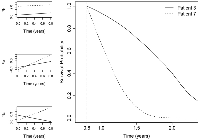
To visualize the prediction and the estimated factor scores of our proposed method, we plot survival probabilities for one comparable pair (patient 3 and patient 7) based on their observations up to 0.8 years, together with their estimated factor scores. Specifically, we estimate ζj(u|t) for some u > t = 0.8 and plot their median survival probabilities, as shown in Figure 8. The GAP scores for patient 3 and patient 7 are 5 and 4, respectively, which suggests that patient 3 has higher risk than patient 7 based on the clinical variable alone. In fact, patient 3 and patient 7 died at 5.2 years and 1.2 years, which contradicts with the prediction using GAP scores. According to the prediction of our model, patient 3 has higher survival probability than patient 7, which is mainly driven by the latent factors as shown in Figure 8. These results suggest that the inclusion of gene expression profiles in the risk prediction model might improve the prediction accuracy and these biomarkers might be more informative than clinical variables.
Fig. 8.
Estimates of the three longitudinal latent factors and the estimated survival probabilities for two patients (patient 3 and patient 7) in the testing data. Plots in the left panel show the estimated factor scores with calculation up to 0.8 years while plot in the right panel shows the estimated survival probabilities for the two patients from 0.8 years to 2.5 years.
6. Discussion
In this paper, we have proposed a new joint modeling method that incorporates the factor analysis model to deal with the longitudinal biomarkers of high dimension and the high correlations among the biomarkers. Our proposed model is similar to the partial least squares regression in that the latent variables are learned in a supervised way, which might lead to increased interpretability of the factors. In the simulation study, we show that our proposed method has improved prediction accuracy compared to the model including only the most informative biomarkers, which might be the first choice of many researchers when a large number of longitudinal biomarkers are presented. The application of our proposed method to the IPF dataset suggests that our method could be very useful, especially in longitudinal genomics studies where there are a large number of longitudinal biomarkers.
We last discuss the limitations of our work and some potential extensions. First, our proposed method only considers the case where the factor scores only include the linear function of time t. However, our method can be easily extended to include nonlinear functions and to include clinical variables in the factor scores, whenever necessary. Second, we have focused on risk prediction and the fitted latent variables η(i)(t) can be interpreted as individual specific scores characterizing both the pattern of gene expression and survival outcome. However, our way to identify informative genes from the factor analysis model is heuristic and may lose information from the loading factor. Consequently, the interpretability of our method could be improved through imposing certain sparsity or group constrain on the loading matrix when certain structure is believed to appear among the biomarkers. This will provide a more systematic way to identity important genes or gene’s group structure. Finally, we have assumed that at all the given time points, we can observe complete longitudinal data. Although this assumption is satisfied for our real data example, it is still possible that biomarkers may be missing when the scale of the study becomes larger and the data quality becomes worse. To the best of our knowledge, there is no existing work dealing with missing values in the joint model. We leave this problem as a potential direction for future work.
Supplementary Material
Acknowledgements
Jiehuan Sun and Hongyu Zhao were supported in part by the National Institutes of Health grants R01 GM59507 and P01 CA154295. Jose D. Herazo-Maya was supported by the Harold Amos Faculty development program of the Robert Wood Johnson Foundation and the Pulmonary Fibrosis Foundation. Naftali Kaminski was supported in part by the National Institutes of Health grants U01 HL108642 and R01 HL127349. The contents are solely the responsibility of the authors and do not necessarily represent the official view of NIH.
Footnotes
Publisher's Disclaimer: This Author Accepted Manuscript is a PDF file of an unedited peer-reviewed manuscript that has been accepted for publication but has not been copyedited or corrected. The official version of record that is published in the journal is kept up to date and so may therefore differ from this version.
Contributor Information
Molei Liu, Department of Biostatistics, Harvard School of Public Health, Harvard University, Boston, MA 02115, U.S.A..
Jiehuan Sun, Department of Biostatistics, Yale University, New Haven, CT 06510, U.S.A..
Jose D. Herazo-Maya, Pulmonary, Critical Care and Sleep Medicine, Yale School of Medicine, New Haven, CT 06519, U.S.A
Naftali Kaminski, Pulmonary, Critical Care and Sleep Medicine, Yale School of Medicine, New Haven, CT 06519, U.S.A.
Hongyu Zhao, Department of Biostatistics, Yale University, New Haven, CT 06510, U.S.A..
References
- Anderson JR, Cain KC, Gelber RD (1983) Analysis of survival by tumor response. Journal of Clinical Oncology 1(11):710–719 [DOI] [PubMed] [Google Scholar]
- Brown ER, Ibrahim JG, DeGruttola V (2005) A flexible B-spline model for multiple longitudinal biomarkers and survival. Biometrics 61(1):64–73 [DOI] [PubMed] [Google Scholar]
- Carvalho CM, Chang J, Lucas JE, Nevins JR, Wang Q, West M (2008) High-dimensional sparse factor modeling: applications in gene expression genomics. Journal of the American Statistical Association 103(484):1438–1456 [DOI] [PMC free article] [PubMed] [Google Scholar]
- Erosheva EA, Curtis SM (2011) Dealing with rotational invariance in Bayesian confirmatory factor analysis Tech. Rep. 589, University of Washington [Google Scholar]
- Faucett CL, Thomas DC (1996) Simultaneously modelling censored survival data and repeatedly measured covariates: a Gibbs sampling approach. Statistics in Medicine 15(15): 1663–1685 [DOI] [PubMed] [Google Scholar]
- Geladi P, Kowalski BR (1986) Partial least-squares regression: a tutorial. Analytica Chimica Acta 185:1–17 [Google Scholar]
- Gelman A, Carlin JB, Stern HS, Rubin DB (2014) Bayesian Data Analysis. Chapman & Hall/CRC Boca Raton, FL, USA [Google Scholar]
- Geweke J, et al. (1991) Evaluating the accuracy of sampling-based approaches to the calculation of posterior moments, vol 196 Federal Reserve Bank of Minneapolis, Research Department Minneapolis, MN [Google Scholar]
- Ghosh J, Dunson DB (2009) Default prior distributions and efficient posterior computation in bayesian factor analysis. Journal of Computational and Graphical Statistics 18(2):306–320 [DOI] [PMC free article] [PubMed] [Google Scholar]
- He Z, Tu W, Wang S, Fu H, Yu Z (2015) Simultaneous variable selection for joint models of longitudinal and survival outcomes. Biometrics 71(1): 178–187 [DOI] [PMC free article] [PubMed] [Google Scholar]
- Herazo-Maya JD, Noth I, Duncan SR, Kim S, Ma SF, Tseng GC, Feingold E, Juan-Guardela BM, Richards TJ, Lussier Y, et al. (2013) Peripheral blood mononuclear cell gene expression profiles predict poor outcome in idiopathic pulmonary fibrosis. Science Translational Medicine 5(205):205ra136–205ra136 [DOI] [PMC free article] [PubMed] [Google Scholar]
- van Houwelingen H, Putter H (2011) Dynamic prediction in clinical survival analysis. CRC Press [Google Scholar]
- Ley B, Ryerson CJ, Vittinghoff E, Ryu JH, Tomassetti S, Lee JS, Poletti V, Buccioli M, Elicker BM, Jones KD, et al. (2012) A multidimensional index and staging system for idiopathic pulmonary fibrosis. Annals of Internal Medicine 156(10):684–691 [DOI] [PubMed] [Google Scholar]
- Press WH (2007) Numerical recipes 3rd edition: The art of scientific computing Cambridge university press [Google Scholar]
- Proust-Lima C, Séne M, Taylor JM, Jacqmin-Gadda H (2014) Joint latent class models for longitudinal and time-to-event data: A review. Statistical Methods in Medical Research 23(1):74–90 [DOI] [PMC free article] [PubMed] [Google Scholar]
- Rizopoulos D (2012) Fast fitting of joint models for longitudinal and event time data using a pseudo-adaptive gaussian quadrature rule. Computational Statistics & Data Analysis 56(3):491–501 [Google Scholar]
- Rizopoulos D, Ghosh P (2011) A Bayesian semiparametric multivariate joint model for multiple longitudinal outcomes and a time-to-event. Statistics in Medicine 30(12):1366–1380 [DOI] [PubMed] [Google Scholar]
- Rizopoulos D, Hatfield LA, Carlin BP, Takkenberg JJ (2014) Combining dynamic predictions from joint models for longitudinal and time-to-event data using Bayesian model averaging. Journal of the American Statistical Association 109(508):1385–1397 [Google Scholar]
- Taylor JM, Park Y, Ankerst DP, Proust-Lima C, Williams S, Kestin L, Bae K, Pickles T, Sandler H (2013) Real-time individual predictions of prostate cancer recurrence using joint models. Biometrics 69(1):206–213 [DOI] [PMC free article] [PubMed] [Google Scholar]
- Tsiatis AA, Davidian M (2004) Joint modeling of longitudinal and time-to-event data: An overview. Statistica Sinica 14(3):809–834 [Google Scholar]
- West M (2003) Bayesian factor regression models in the “large p, small n” paradigm In: Bernardo J, Bayarri M, Dawid A, Heckerman D, Smith A, West M (eds) Bayesian Statistics, vol 7, Oxford University Press, pp 723–732 [Google Scholar]
Associated Data
This section collects any data citations, data availability statements, or supplementary materials included in this article.


