TaxoNN: ensemble of neural networks on stratified microbiome data for disease prediction

Abstract

Motivation

Research supports the potential use of microbiome as a predictor of some diseases. Motivated by the findings that microbiome data is complex in nature, and there is an inherent correlation due to hierarchical taxonomy of microbial Operational Taxonomic Units (OTUs), we propose a novel machine learning method incorporating a stratified approach to group OTUs into phylum clusters. Convolutional Neural Networks (CNNs) were used to train within each of the clusters individually. Further, through an ensemble learning approach, features obtained from each cluster were then concatenated to improve prediction accuracy. Our two-step approach comprising stratification prior to combining multiple CNNs, aided in capturing the relationships between OTUs sharing a phylum efficiently, as compared to using a single CNN ignoring OTU correlations.

Results

We used simulated datasets containing 168 OTUs in 200 cases and 200 controls for model testing. Thirty-two OTUs, potentially associated with risk of disease were randomly selected and interactions between three OTUs were used to introduce non-linearity. We also implemented this novel method in two human microbiome studies: (i) Cirrhosis with 118 cases, 114 controls; (ii) type 2 diabetes (T2D) with 170 cases, 174 controls; to demonstrate the model’s effectiveness. Extensive experimentation and comparison against conventional machine learning techniques yielded encouraging results. We obtained mean AUC values of 0.88, 0.92, 0.75, showing a consistent increment (5%, 3%, 7%) in simulations, Cirrhosis and T2D data, respectively, against the next best performing method, Random Forest.

Availability and implementation

https://github.com/divya031090/TaxoNN_OTU.

Supplementary information

Supplementary data are available at Bioinformatics online.

1 Introduction

The human microbiome comprises a collection of microbes which live on and inside the human body. The microbiome data are usually quantified into Operational Taxonomic Units (OTUs), based on their sequence similarity to reference datasets (Blaxter et al., 2005). The risk of some diseases has been found to be associated with the host’s microbiome (Jackson et al., 2018), making prediction of risk of disease based on microbiome analysis an important problem. In this regard, machine learning can efficiently understand the relationship between the microbiomes and between microbiomes and diseases (Sommer et al., 2017).

The role of the microbiome has been examined in subjects with a variety of diseases such as Inflammatory Bowel Diseases (Gevers et al., 2014), Cirrhosis (Schnabl and Brenner, 2014) and type 2 diabetes (T2D) (Hartstra et al., 2015) justifying the potential use of the microbiome as a disease risk prediction tool. A sparse distance-based learning method for multiclass classification of human microbiota is proposed by Liu et al. (2011); Pasolli et al. (2016) proposed a computational framework for prediction tasks using species-level relative abundances and strain-specific markers. Whereas, Bokulich et al. (2018) presented a comparison of supervised learning classifiers and regressors for microbiomes using a Python-based machine-learning library. Ananthakrishnan et al. (2017) incorporated clinical and microbiome data to classify treatment response and Lo and Marculescu (2019) proposed a neural network framework for disease prediction with data augmentation to mitigate over-fitting. However, the role of taxonomy in prediction using OTU data is often unclear, wherein similar OTUs are often correlated across samples.

Convolutional Neural Networks (CNNs) (Krizhevsky et al., 2012) have been successfully applied to diversified areas such as face recognition (Yang et al., 2016), optical character recognition (Bai et al., 2014) and medical diagnosis (Sun et al., 2016). CNNs perform well in capturing spatial and temporal dependencies in the input data. CNNs are also capable to capture interactions in the data during prediction (Tsang et al., 2017). Ensemble learning has also garnered a lot of attention in the field of bioimage classification (Nanni et al., 2018) and scene-text recognition (Park et al., 2016) wherein multiple neural networks are combined together to enhance model performance as well as incorporate multiple inputs. However, we observed that CNNs have not been widely applied in the area of microbiome analysis to predict disease risk. One reason could be that OTU relative abundance data in itself (without any re-arrangement) does not show any spatial similarity that the CNNs can capture.

Motivated by the inherent correlation shared by the OTUs in the same taxonomy level and the non-linear relationship between the OTUs during disease prediction (Tsai et al., 2015; Xiao et al., 2018), we propose a novel deep learning model taxoNN (taxonomy-based Neural Network). taxoNN stratifies input OTU data into various clusters based on their phylum information. Further, as ensemble learning is effective, hence, we propose an ensemble of CNNs over the stratified clusters containing OTUs sharing the same phylum. The rationale is that OTUs after the phylum level division share similarity and hence, some correlation with each other. Moreover, to introduce spatial relationship in the input OTUs for the CNNs to capture, we order the OTUs on the basis of correlation with each other and Euclidean distance from the centre of the cluster.

2 Materials and methods

2.1 Proposed neural network framework: taxoNN

We experimented with using three types of CNN models. To begin with, we used a basic convolutional framework (CNN_basic), where the input OTUs were arranged in an alphabetical order of their taxonomic label and hence, their order did not represent a biological relationship.

We then experimented with shuffling the OTUs (CNN_shuffle) in the input on each iteration of the neural network, in the assumption that the various iterations of shuffling would in turn lead to correlated microbiomes arrange in one window. However, this assumption might limit the prediction accuracy.

Hence, we finally examined incorporating the inherent phylogenetic relationship in the OTU data before providing it as an input to the neural network model. Supplementary Figure S1, shows a sample taxonomy tree containing various taxonomic levels and illustrates that hierarchy in OTU data is complex and clusters corresponding to the different phyla can contain a varied number of OTUs.

Let there be ‘I’ subjects in the whole study, the OTU data for ith subject (where, $i\in$ I), was presented in a 1-D vector format to the network, as, ${\text{OTU}}_{i\text{th}\hspace{0.17em}\text{subject}}=\{o_1,o_2,\dots ,o_N\}$, where, N was the total number of OTUs in a subject. These OTUs were then stratified into four clusters based on their phyla such that each cluster had different number of OTUs. For example the first cluster contained ‘p’ OTUs, second contained ‘q’ OTUs, third contained ‘r’ OTUs and fourth contained ‘s’ OTUs (where p + q+r + s = N), and CNN was applied to each cluster individually. To order and place correlated OTUs together, we adopted two approaches:

Approach 1: Ordering based on distance to the cluster centre: In this approach, for a cluster, we took ‘p’ OTUs of I-dimension each (corresponding to ‘I’ number of subjects), inside the cluster. We then calculated the medoid of that cluster. A medoid is a representative object of a dataset whose average dissimilarity to all the objects in the cluster is minimal. A medoid in a cluster containing OTUs of the same phyla, is calculated using the formula:

$${\text{OTU}}_{\text{medoid}}={\text{argmin}}_{y\in \{{\text{OTU}}_1,{\text{OTU}}_2,\dots ,{\text{OTU}}_p\}}\sum _{j=1}^{p}d(y,{\text{OTU}}_j)$$ (1)

As can be seen in Supplementary Figure S12a, for ease of representation, we took a few OTUs and considered their OTU vectors to contain only three subjects. OTUs are shown as blue dots representing relative abundance of that particular OTU and medoid of these OTUs was then calculated (shown as red dot Supplementary Fig. S12b) using Equation 1. Further, Euclidean distances d_i, d_j and d_k of three sample OTUs (i, j and k) from the medoid were calculated (Supplementary Fig. S12c) and OTUs were ordered on the basis of their increasing distance to the medoid. In this way, we obtained $d_i<d_j<d_k$, therefore, OTU_i was ordered before OTU_j and OTU_k in the OTU vector that was provided as an input to the CNN. This idea was extended to all the ‘p’ OTU vectors in the cluster.

This ordering combined with the convolutional sliding window helped to combine OTUs which were closely located and shared more similarity in the cluster. OTUs in the same sliding window, combined with the weight vector in the neural network led to creating non-linear terms that were sent to the next layer of the neural network and hence, this helped in understanding the non-linear relationship between them. We named this variation of taxoNN as taxoNN_dis.

Approach 2: Ordering based on correlation: The second approach that we used was to order the OTUs based on their correlation with each other using Spearman rank. This gave us a p × p matrix for p OTUs in a cluster as shown in Figure 1a. Next, each row of this correlation matrix was reduced to a cumulative correlation coefficient, calculated with respect to all the OTUs in a single row using the formula:

$${\rho }_{{\text{OTU}}_{{\text{row}}_j}}=\sqrt[p]{\left|{\rho }_{{\text{OTU}}_{j1}}\right|·\left|{\rho }_{{\text{OTU}}_{j2}}\right|\cdots \left|{\rho }_{{\text{OTU}}_{jp}}\right|}$$ (2)

for $j\in [1,p]$

Fig. 1.

An illustration of correlation-based ordering in the OTUs in a cluster. (a) Example heatmap obtained by plotting Spearman rank coefficients between positively correlated OTUs in a cluster. (b) Cumulative coefficient obtained with respect to each row of the heatmap matrix. (c) Vector of cumulative coefficients arranged in a decreasing order where, ${\rho }_{{\text{OTU}}_{\text{row}5}}>{\rho }_{{\text{OTU}}_{\text{row}3}}>{\rho }_{{\text{OTU}}_{\text{row}p}}>{\rho }_{{\text{OTU}}_{\text{row}1}}>{\rho }_{{\text{OTU}}_{\text{row}k}}$. (d) The cumulative coefficients are renamed as ${\rho }_{{\text{OTU}}_{{\text{row}}_i}^{*}}$ to represent that they are now arranged in a decreasing order. (e) Heatmap sorted based on the new order of cumulative coefficients, making the correlated terms concentrate in a space and arrange closer in the matrix

The set of these cumulative coefficients is represented as $P_{\text{OTU}}$ (Fig. 1b) as:

$$P_{\text{OTU}}=\{{\rho }_{{\text{OTU}}_{{\text{row}}_1}},{\rho }_{{\text{OTU}}_{{\text{row}}_2}},\dots ,{\rho }_{{\text{OTU}}_{{\text{row}}_p}}\}$$ (3)

Thus, we obtained a vector of correlation coefficients, $P_{\text{OTU}}$ based on Equation 3, with each value representing a cumulative correlation coefficient for each row. The values in the set $P_{\text{OTU}}$ were then arranged in a decreasing order and a new vector $P_{\text{OTU}}^{*}$ was created containing cumulative correlation coefficients in decreasing order which were further re-indexed from 1 to p. The asterisk here represents re-indexing.

$$P_{\text{OTU}}^{*}=\{{\rho }_{{\text{OTU}}_{\text{row}5}},{\rho }_{{\text{OTU}}_{\text{row}3}},\dots ,{\rho }_{{\text{OTU}}_{{\text{row}}_k}}\}$$ (4)

 

$$P_{\text{OTU}}^{*}=\{{\rho }_{{\text{OTU}}_{{\text{row}}_1}}^{*},{\rho }_{{\text{OTU}}_{{\text{row}}_2}}^{*},\dots ,{\rho }_{{\text{OTU}}_{{\text{row}}_p}}^{*}\}$$ (5)

Subsequently, the heatmap obtained by the correlations in the OTU data is reordered based on the decreasing order of the cumulative correlation coefficients. Through this ordering the correlation structure between the OTUs was used to establish a similarity in the neighbouring OTUs before being provided to the neural network model. We named this variation of taxoNN as taxoNN_corr.

The broad overview of our CNN framework is presented in Figure 2a. Figure 2b illustrates various layers in the neural network acting on each cluster of the OTU data. We defined the model with two 1-D convolutional layers, each followed by a pooling layer. The data has been pre-processed in such a way that each vector contains N OTUs. These OTUs are then divided into clusters based on their phylum level with first cluster containing ‘p’ OTUs, second containing ‘q’ OTUs, third containing ‘r’ OTUs and fourth containing ‘s’ OTUs. The first convolutional layer (Conv1) defines 32 filters (feature detectors) of height 5 (window size) and stride size (number by which sliding window slides) of 1. For activation, we use Rectified Linear Unit (ReLU) (Glorot et al., 2011) and after the convolution operation (Krizhevsky et al., 2012) in the first layer, the extracted features were forwarded to the pooling layer (Pool1). A pooling layer is often used after a CNN layer in order to reduce the complexity of the output and prevent overfitting of the data. Similarly, a second set of convolutional (with 64 filters) and pooling Layer (Conv2 and Pool2) were used to extract features. Finally, the feature vectors obtained were flattened to a single vector. In a similar manner features were learned and flattened from each cluster.

Fig. 2.

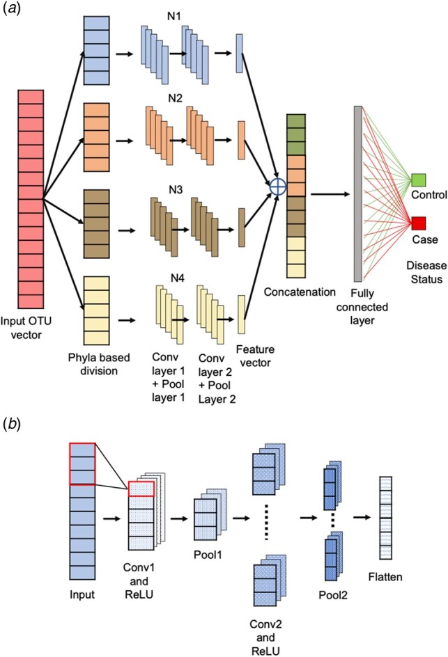
Illustration of the layers in the CNN framework. (a) Detailed illustration of the phylum-based stratification and ensemble learning of CNNs for disease prediction. The four different clusters are color coded with different colours and after phyla stratification are input to the four neural networks (N1, N2, N3 and N4). Later the features extracted are flattened and stacked during the concatenation step to further lead to prediction of disease outcome. (b) Illustration of the layers in a single neural network (N1/N2/N3/N4) acting on one particular cluster of the input data. (Color version of this figure is available at Bioinformatics online.)

Next, ensemble learning (Hansen and Salamon, 1990) was used, where, features from each cluster were combined. The flattened vectors obtained from each cluster were merged via concatenation to make one very long vector that was then interpreted and sent to two fully connected layers before a prediction was made. In the two fully connected layers the first layer had 100 nodes followed by a ReLU activation while the second layer had only a binary node with a softmax activation (Goodfellow et al., 2016) to predict the two classes according to the disease status (Disease/Control). The details about the input and output processing through each layer are shown in Supplementary Figure S19. We also experimented with adding variables such as age and sex as input along with the OTU data in the model. In this scenario, two separate vectors, one containing age values and other, the sex values were given as input to the individual CNNs along with the OTU vectors in each cluster.

2.2 Simulated studies

We designed simulation studies using the microbiome data available in the ‘Genetic, Environmental, Microbial’ (GEM) project (Turpin et al., 2016). Subjects were first-degree relatives of subjects with Crohn’s disease between 6 and 35 years of age and recruited between 2008 and 2015. This project aimed to identify microbial, genetic and environmental factors responsible for the initiation of Crohn’s disease. Stool samples were collected for 16S ribosomal DNA sequencing at a minimum depth of 30 000 reads/sample. Samples with fewer than 30 000 reads and OTUs with prevalence of $<5\%$ were removed from the analysis. Analysis was restricted to merged OTUs with the same taxonomic assignment.

Our simulated datasets were created using 1796 subjects provided in the GEM study data. Each sample contained values for 168 OTUs. The OTUs in this simulated dataset were categorized into taxonomy levels with 12 phyla, 15 classes, 20 orders, 37 families and 60 genera. The three dominant bacterial phyla in terms of the number of OTUs were Firmicutes, Proteobacteria and Actinobacteria.

We used this data to create a population with 100 000 samples. Instead of a simple replication we added noise to each OTU using a normally distributed function with mean equal to a random number in the range $[1\times {10}^{-6},2\times {10}^{-6}]$ and standard deviation of ${10}^{-6}$ to create new samples. While doing so we ensured that we preserve the zeroes and also considered that the relative abundance is equal to one, by adding and subtracting the noise term in equal proportion in each OTU set, keeping the zeroes. We then generated the disease status (y = 1 for case; y = 0 for control) using the formula:

$$p(y=1)=\frac{\hspace{0.17em}\text{exp}(\alpha +\sum _{i=1}^{32}{\beta }_i·{\text{OTU}}_i+\sum _{i=1}^2\sum _{j=i+1}^3{\beta }_{ij}·{\text{OTU}}_i·{\text{OTU}}_j)}{1+\text{exp}(\alpha +\sum _{i=1}^{32}{\beta }_i·{\text{OTU}}_i+\sum _{i=1}^2\sum _{j=i+1}^3{\beta }_{ij}·{\text{OTU}}_i·{\text{OTU}}_j)}$$ (6)

where β_i were the regression coefficients associated with OTUs, α was the base prevalence, β_ij were the regression coefficients for the pairwise interaction terms, y was the outcome variable and $p(y=1)$ was the probability of the outcome variable to be 1, i.e. disease status positive. In general, the OTUs that are potentially associated with risk of disease, in a microbiome dataset are unknown and their number can range from zero to a very large value. Carefully choosing the number of these OTUs during simulating data, thus, becomes a challenge. Therefore, based on a trade-off between the model performance upon analysis with various number of OTUs (Supplementary Table S1) and the realistic estimation of OTUs potentially associated with risk of disease in a real microbiome dataset, we selected 32 OTUs randomly as the OTUs that were potentially associated with risk of disease, also ensuring that all clusters contribute to these OTUs. We set the value of α as -2.5, β_i in 1st cluster ranging from [1,1.5], 2nd cluster ranging from [1,2], 3rd cluster ranging from [1.5,2] and 4th cluster [0.5,1]. Interaction terms were added to introduce non-linearity in the data. Out of the 32 OTUs potentially associated with risk of disease, 3 OTUs were randomly picked and three pairwise interactions between them were generated (as shown in Equation 6), where, β_ij was taken as [1,1.5,2]. In this way, we generated 2000 samples as cases and 98 000 as controls from the 100 000 samples. For the simulation data to evaluate our algorithm, we then randomly selected 200 cases from theses 2000 case samples and randomly selected 200 matched controls based on age and sex. We performed 1:1 matching of cases to controls for age in the range of ±5 years and exact match for sex. Hence, obtained a case-control dataset of 200 cases and 200 controls. 100 simulation datasets were generated following the same strategy.

The phyla-based stratification on the OTUs in the simulated dataset was done in the following manner: for 168 OTUs, after phyla-based stratification, 1st cluster contained 92 OTUs, 2nd contained 28 OTUs, 3rd contained 27 OTUs and 4th contained 21 OTUs. Each cluster was provided as an input to an individual CNN to understand the relationships between OTUs inside each phyla and later the extracted features were used for making the predictions.

2.3 Real studies: T2D study and Cirrhosis study

To assess the prediction power of taxoNN on linking the gut microbiome with disease risk, we implemented our algorithm on a T2D (Qin et al., 2012) study containing 174 cases and 170 controls and a liver Cirrhosis study (Qin et al., 2014), containing 118 cases and 114 controls. OTUs at the genus level in the kingdom ‘Bacteria’ were used as an input. The T2D data was based on deep next-generation shotgun sequencing of DNA extracted from the stool samples from Chinese subjects. The subjects in the Cirrhosis data were of Han Chinese origin. In both studies Proteobacteria, Actinobacteria and Firmicutes emerged as the phyla with majority of OTUs, leading to forming three major clusters for taxoNN. Supplementary Tables S2 and S3 give more details about the OTUs in each cluster in the T2D study and Cirrhosis study, respectively. Details of variables like age and sex of the subjects provided with both studies are given in Supplementary Table S4. The box-plots containing relative abundance percentages of OTUs in each phylum of T2D and Cirrhosis studies are presented in Supplementary Figures S3 and S7, respectively. Supplementary Figures S4–S6 and Supplementary Figures S8–S10 provide box-plots for relative abundance percentages of genera in each cluster of the T2D and Cirrhosis studies.

2.4 Model specification and evaluation criteria

For training the neural network model on the simulated study, 70% of the subjects were considered in the training data and 30% in the test data. Therefore, out of 200 controls and cases which were pair-matched for age and sex as described in Section 2.2, 140 controls and 140 cases were used for training the network, and 60 controls and 60 cases were used for testing the network. Similarly, for the T2D and Cirrhosis studies, 70% of the subjects were considered in the training data and, 30% in the test data. Thereby, in the T2D study 119 cases and 119 controls were used for training and 55 cases and 50 controls were used for the test set. In Cirrhosis study, 83 controls and 83 cases were used for training and 31 controls and 35 cases were used to test the model. We also performed an internal validation using 10 times 10-fold cross validation on the training set itself, to analyze model performance before testing and to eliminate overfitting. For the cross-validation, we used 90% of the total training set selected at random for training, and the remaining 10% as a hold out set for testing. We obtained 10 AUC values corresponding to initial 10-folds in the training set. We repeated this process 10 times in order to generate corresponding 100 AUC values. We then calculated the 95% confidence intervals using these 100 AUC values. 400 epochs were run for the neural network model with a stride size of 1, window size of 5, number of OTUs related to disease outcome set as 32 for the first layer and number of filters in the CNN network as 32. Each network was trained using stochastic gradient descent with a learning rate of 0.001. We trained our network on an NVIDIA Tesla P100 GPU with 16GB of RAM using tensorflow library in Python alongwith some data analysis using R version 3.5.3.

The performance of our technique was evaluated through a Receiver Operating Characteristics curve (ROC curve) using specificity, sensitivity and thereafter calculating mean Area Under Curve (AUC), where a larger AUC meant a better classification model. Given the number of true positives (TP), false positives (FP), true negatives (TN) and false negatives (FN), the measures are mathematically expressed as follows: Sensitivity=TP/(TP+FN) and Specificity=TN/(TN+FP).

We compared the results obtained by our proposed model taxoNN in its two variations taxoNN_dis and taxoNN_corr against conventional machine learning models like Random Forests (RFs) (Liaw et al., 2002), Gaussian Bayes Classifier (GBC) (Hand and Yu, 2001), Naive Bayes (NB) (Rish et al., 2001), Ridge regression (Hoerl and Kennard, 1970), Lasso regression (Tibshirani, 1996) and Support Vector Machines (SVM) (Suykens and Vandewalle, 1999).

3 Results

3.1 Simulation results

3.1.1. Type 1 error performance

In the simulated datasets, first, we tested for taxoNN under the null, i.e. where none of the OTUs in the input data were related to the outcome i.e. disease status. We obtained an AUC value of 0.513 using taxoNN_corr and 0.504 with taxoNN_dis model. Comparing the AUC values obtained from our model with RF (AUC = 0.502), SVM (AUC = 0.523), Ridge (AUC = 0.517) and Lasso (AUC = 0.510) we observed that our model was stable under the null and shows that the prediction of disease status was not governed by the OTUs in the case of non-causal relationship between the OTUs and disease.

3.1.2. Comparison of predictive performance

For the simulated datasets under the situation of association, the ROC curves obtained are presented in Figure 3. As can be seen in Figure 3, the blue and the brown plot lines in the graph depict the ROC curve for taxoNN_corr and taxoNN_dis, respectively. The area under the curve was highest for our proposed models, taxoNN_corr and taxoNN_dis with AUC values, 0.883 and 0.874, respectively, followed by RF technique (AUC = 0.846). As discussed, we initially experimented with predicting disease status using a basic CNN model. As the arrangement of input OTU data in this case did not signify any relationships, therefore, the AUC obtained was equal to 0.753. The second variation we tried was to shuffle the input data on each iteration of the CNN (CNN_shuffle) so that, we can approximate OTU correlations by making them fall in the same CNN window for combination into the next layer. We observed that, in this case the performance of the CNN improved (AUC = 0.822), as compared to the basic CNN. However, the performance in this method is highly dependent upon the OTU combinations resulting due to the shuffling and thus, might vary upon shuffling the OTUs. The other machine learning methods like RF and SVM with AUCs 0.846 and 0.825, respectively, performed relatively better than GBC and NB (AUC = 0.792, 0.789, respectively) due to their tree-based structure, rendering their ability to capture non-linearity in the data. However, there was a clear under-performance by these methods as compared to taxoNN_corr with a difference in AUC ranging from about 0.038 for RF and increasing to about 0.094 for the least efficient performing method GBC. The computation time taken by our method on an NVIDIA Tesla P100 GPU with 16GB of RAM for each iteration of the ensemble of neural networks was 9.35 s. The initial ordering of the input OTU data took 1.27 s. Therefore, each iteration took about 10.62 s. The neural networks ran simultaneously for each cluster and took 400 epochs to learn, therefore, the overall time taken for taxoNN to train was about 70.8 min for the simulated dataset. Details of the performance of taxoNN in case of change in parameters associated with the neural network, in presence of interaction terms and in case of imbalance of case and controls is shown in Supplementary Table S1, Supplementary Table S5 and Supplementary Figure S11, respectively.

Fig. 3.

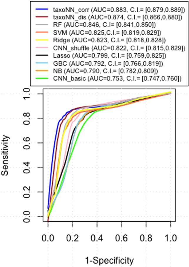
ROC curve obtained on the test set of the simulated study. The test set comprised 60 controls and 60 cases. The red dotted line corresponds to AUC equal to 0.5, indicating a random classification model

3.2 Results for T2D and Cirrhosis studies

In this section, we present results on the training and test sets of the T2D and Cirrhosis studies. We filtered the data in both the studies, eliminating OTUs that had a zero proportion in all individuals and thereby obtained 184 OTUs for the Cirrhosis study and 208 for the T2D study after this filtering. Supplementary Figure S2 illustrates pie-charts corresponding to the OTU distribution in the T2D and Cirrhosis studies. Illustration of how the heatmaps are sorted and rearranged based on the correlations between the OTUs in each cluster are provided in Supplementary Figures S13–S15 for T2D and Supplementary Figures S16–S18 for Cirrhosis study. An additional analysis on an external validation cohort (Karlsson et al., 2013) is presented in Supplementary Tables S7 and S8.

3.2.1. Results for T2D study

The results for T2D dataset taking 10-fold cross validation on the training set are presented in Figure 4a (also, Supplementary Table S6). We plotted the 95% confidence intervals (CI) for each of the methods. The mean AUC values obtained for taxoNN and taxoNN were 0.753 (95% CI: 0.741–0.761) and 0.741 (95% CI: 0.731–0.750), respectively, followed by RF (AUC = 0.740), CNN_shuffle (AUC = 0.736), SVM (AUC = 0.721), Ridge regression (AUC = 0.699), Lasso regression (AUC = 0.687), GBC (AUC = 0.684) and NB (AUC = 0.682). We also calculated the results on the test set of the T2D study (tabulated in Table 1 second column), and obtained a mean AUC value of 0.733 using taxoNN_corr which was considerably higher than the other machine learning methods on the test set.

Fig. 4.

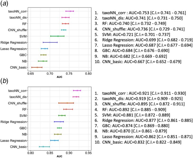
95% confidence intervals obtained for the mean AUC values for 10 times 10-fold cross validation on the training set for the (a) T2D study and the (b) Cirrhosis study

Table 1.

AUC values tabulated for various machine learning methods on test set of T2D and Cirrhosis studies

	AUC T2D		AUC Cirrhosis
Method	w/o age+sex	w age+sex	w/o age+sex	w age+sex
RF	0.703	0.708	0.893	0.901
GBC	0.642	0.648	0.816	0.825
SVM	0.701	0.704	0.877	0.882
Lasso regression	0.665	0.670	0.823	0.831
Ridge regression	0.700	0.705	0.842	0.848
NB	0.682	0.685	0.802	0.807
CNN_basic	0.643	0.647	0.799	0.801
CNN_shuffle	0.712	0.718	0.844	0.852
taxoNN dis	0.720	0.725	0.903	0.908
taxoNN corr	0.733	0.762	0.911	0.938

Note: The results are reported on both studies considering model performance without (w/o) including age and sex and with (w) age and sex. Note that the last row (values in bold) shows the consistent improvement in the performance of the proposed model taxoNN_corr for both studies.

3.2.2. Results for Cirrhosis study

The results for Cirrhosis study taking 10 times 10-fold cross validation by creating 10-folds in the training set and using 1 out of the 10-folds for testing each time are presented in Figure 4b (also, Supplementary Table S6). The 95% confidence interval over the 100 mean AUC values were calculated for the other machine learning methods in comparison to taxoNN. We obtained a mean AUC value as high as 0.921 (95% CI: 0.911–0.930) for the proposed taxoNN_corr model closely followed in performance by the taxoNN_dis model with a mean AUC of 0.919 (95% CI: 0.909–0.925). An improvement of 0.025 was noted when comparing the AUC value of taxoNN_corr to the next best performing method of RF (AUC = 0.892) followed by the SVM method which was observed to give a mean AUC of 0.881. The GBC, NB and Ridge regression performed comparably with mean AUC values of 0.874, 0.870 and 0.877, respectively. It was observed that the least efficient method in this case was the basic CNN model with AUC as low as 0.832. Results on the test set for Cirrhosis study are reported in Table 1, fourth column, showing the effectiveness of taxoNN on the Cirrhosis study.

3.2.3. Incorporating clinical variables

As tabulated in Supplementary Table S4, we observed that in both studies cases were significantly older than the controls. In the T2D study the cases had a significantly greater proportion of males than controls. Whereas, for Cirrhosis study, there were no significant differences in sex between cases and controls. To analyze further, we evaluated the prediction power of our model including age and sex data. We observed an AUC value of 0.592 given the age and sex for the Cirrhosis dataset using logistic regression. Similar, observation was made for the T2D dataset where we obtained an AUC value of 0.613 using just the age and sex. When we combined these two variables along with the OTU training set (performing 10 times 10-fold validation) and provided it as input (Table 1 third column) to taxoNN_corr for the T2D study, we obtained an improved AUC of 0.762 as compared to 0.738 previously obtained using only the OTUs. The same held valid for the Cirrhosis study, where the AUC after combining environmental variables increased from 0.921 to 0.938 (Table 1 fifth column). We also observed that when age and sex were provided to other machine learning models of the T2D study, enhanced their performance a little, with an increase of 0.008, 0.009, 0.005, 0.008, 0.006, 0.005 in the AUC values of RFs, SVM, GBC, NB, Lasso Regression, Ridge Regression, respectively (Table 1). A similar trend was observed for the performance in Cirrhosis study, with an increase of ∼0.005 in AUC values for other machine learning methods. However, it is to be noted that in taxoNN, inclusion of age and sex enhanced the performance to a larger degree as compared to other machine learning methods (increase of 0.017 and 0.009 in the AUC in T2D and Cirrhosis studies, respectively).

4 Discussion

Extensive analysis on three datasets establish that stratifying OTU data into clusters and using ensembles of CNN models on the clusters to predict disease status as proposed in taxoNN leads to efficiently capturing OTU data. We observed that taxoNN performs consistently better across all the three datasets. Other methods like RFs which have a record of working well with non-linear data (Ryo and Rillig, 2017), performed slightly better than NB and GBC methods while predicting the risk of disease (Table 1). We also observed that in general, the AUC values obtained by performing 10 times 10-fold validation on the training set (Supplementary Table S6) were higher than the one obtained by working on the test set (Table 1).

By changing the parameters associated with the CNN (Supplementary Table S1) such as window size and the number of filters in each layer, we observed a trend of dropping in performance upon increasing these parameters beyond a certain level. We inferred that up to window size of five the performance was good, but increasing the window size further resulted in adding unnecessary amount of correlations between the OTUs in the input data which might not truly reflect the scenario in the real data. Similarly, when we increased the number of filters from 32 to 64 we observed that the performance dropped.

We also analyzed the methods in the literature that propose machine learning techniques for disease prediction for T2D and Cirrhosis studies. Qin et al. (2014) used an SVM method with training set (AUC of 0.918) and leave-one-out cross-validation set (AUC of 0.838) for the Cirrhosis data. In comparison, taxoNN_corr using the 10-fold cross validation outperformed by a significant margin giving an AUC value of 0.921 and similarly, taxoNN_dis also gave a much higher AUC of 0.919 suggesting our model’s efficiency. Qin et al. (2012) propose a T2D classifier system based on the 50 gene markers through a minimum redundancy–maximum relevance (mRMR) feature selection method, to exploit the potential ability of T2D classification by gut microbiota. An AUC of 0.81 was reported using SVM for classification through the gene markers. As our model focused on relative abundance of the OTUs, therefore, a straight comparison to the results provided by Qin et al. (2012) was not feasible.

However, there are a few assumptions and limitations of our method. Microbiomes can reside in various sites in the body such as skin, mammary glands, uterus, ovarian follicles, oral mucosa and gut. However, for the scope of this article, we implemented our algorithm only on gut microbiome data, limiting our analysis to predicting diseases caused by gut microbiomes. As discussed earlier, the OTUs that are potentially associated with risk of disease in a microbiome dataset are unknown and their number in a study can be arbitrary, ranging from zero to a very large value. We experimented with taking 8, 16 and 32 OTUs associated to disease outcome in the simulation study, which ranges from 5 to 15% of the total OTUs in the study. We then selected 32 OTUs as the OTUs associated with risk of disease based on their performance in taxoNN (Supplementary Table S1). However, we might be under or over estimating the number of OTUs and it would be interesting to consider different number of OTUs in the future to evaluate the model better. Also, we simulated the data, taking three interaction terms w.r.t three randomly selected OTUs to add non-linearity in our OTU data. However, just three pairs of OTUs might not be enough to approximate the complex relationship presented within real OTU data. Hence, a better analysis by varying the number of interacting OTUs needs to be done to evaluate model performance. For our analysis, we consider phylum level stratification in taxoNN in all the three studies, due to presence of adequate number of OTUs in phylum level which is required for efficient model training. However, in the future, it will be interesting to observe studies which have adequate OTUs in other taxonomy levels like class and order along with phylum level (Supplementary Table S9).

As tabulated in Supplementary Table S4, age has been identified to be associated with the disease outcome for both T2D and Cirrhosis, whereas sex has been identified to be associated with T2D. This may represent poorly matched subjects in these studies. If these factors are causally associated with disease, then when used along with OTU data, they can enhance the performance of the model. However, our model is currently limited to just these two variables alongside the OTU data. A more comprehensive analysis taking other environmental variables like ethnicity, smoking status, dietary habits and medication can be conducted to evaluate their effects in disease prediction alongside microbiome data. We also observed that our method performs fairly robustly with respect to imbalance in the number of cases and controls up to a certain level (Supplementary Fig. S11), but the performance dropped considerably when the imbalance increased (1:4 ratio between cases and controls). Hence, better techniques to handle data imbalance need to be examined.

5 Conclusion

We propose a technique to predict disease status through gut microbiome data using a novel ensemble of neural networks. Using the inherent biological information in the OTU data, we divided the OTUs into clusters based on their phylum and trained on each cluster individually and later ensembled features from each neural network to predict disease status. We also proposed two novel ordering methods based on correlation and cluster centre distance to arrange input OTUs based on their similarity to help capture the spatial similarity in the input as required by the CNN. We obtained encouraging results on simulation data, Cirrhosis and T2D studies and consistent improvement in performance across both test and training sets compared to competing methods.

From our analysis we can infer, that non-linearity in the OTU data can be captured well using a CNN and relationships provided by the taxonomy in OTU data can help to improve accuracy of disease prediction. In the future, we would like to apply taxoNN for predicting continuous and time-to-event outcomes in addition to the current binary outcome and potentially implement our model on pathway analysis in genetic data. We would aim to identify specific microbiomes which play an important role for causing a particular disease. The limitations discussed in Section 4, pertaining to dealing with imbalance in input data and experimenting with more interaction terms also provide a good scope for future studies.

Funding

Wei Xu was funded by Natural Sciences and Engineering Research Council of Canada (NSERC Grant RGPIN-2017-06672), Crohn’s and Colitis Canada (CCC Grant CCC-GEMIII), and Helmsley Charitable Trust. Divya Sharma was supported by NSERC Grant RGPIN-2017-06672 and CCC Grant CCC-GEMIII.

Financial Support: none declared.

Conflict of Interest: none declared.

References

- Ananthakrishnan A.N. et al. (2017) Gut microbiome function predicts response to anti-integrin biologic therapy in inflammatory bowel diseases. Cell Host Microbe, 21, 603–610. [DOI] [PMC free article] [PubMed] [Google Scholar]
- Bai J. et al. (2014) Image character recognition using deep convolutional neural network learned from different languages. In Proceedings of the IEEE International Conference on Image Processing, pp. 2560–2564. IEEE.
- Blaxter M. et al. (2005) Defining operational taxonomic units using DNA barcode data. Philos. Trans. R. Soc. B Biol. Sci., 360, 1935–1943. [DOI] [PMC free article] [PubMed] [Google Scholar]
- Bokulich N.A. et al. (2018) q2-sample-classifier: machine-learning tools for microbiome classification and regression. J. Open Res. Softw., 3, 934. [DOI] [PMC free article] [PubMed] [Google Scholar]
- Gevers D. et al. (2014) The treatment-naive microbiome in new-onset Crohn’s disease. Cell Host Microbe, 15, 382–392. [DOI] [PMC free article] [PubMed] [Google Scholar]
- Glorot X. et al. (2011) Deep sparse rectifier neural networks. In Proceedings of the Fourteenth International Conference on Artificial Intelligence and Statistics, JMLR, W&CP (15), pp. 315–323.
- Goodfellow I. et al. (2016) Deep Learning. MIT Press, Cambridge, MA. [Google Scholar]
- Hand D.J., Yu K. (2001) Idiot’s Bayes—not so stupid after all? Int. Stat. Rev., 69, 385–398. [Google Scholar]
- Hansen L.K., Salamon P. (1990) Neural network ensembles. IEEE Trans. Pattern Anal. Mach. Intell., 12, 993–1001. [Google Scholar]
- Hartstra A.V. et al. (2015) Insights into the role of the microbiome in obesity and type 2 diabetes. Diabetes Care, 38, 159–165. [DOI] [PubMed] [Google Scholar]
- Hoerl A.E., Kennard R.W. (1970) Ridge regression: biased estimation for nonorthogonal problems. Technometrics, 12, 55–67. [Google Scholar]
- Jackson M.A. et al. (2018) Gut microbiota associations with common diseases and prescription medications in a population-based cohort. Nat. Commun., 9, 1–8. [DOI] [PMC free article] [PubMed] [Google Scholar]
- Karlsson F.H. et al. (2013) Gut metagenome in European women with normal, impaired and diabetic glucose control. Nature, 498, 99–103. [DOI] [PubMed] [Google Scholar]
- Krizhevsky A. et al. (2012) Imagenet classification with deep convolutional neural networks. In: Advances in Neural Information Processing Systems, Curran Associates, Inc., NY, US, pp. 1097–1105.
- Liaw A. et al. (2002) Classification and regression by RandomForest. R News, 2, 18–22. [Google Scholar]
- Liu Z. et al. (2011) Sparse distance-based learning for simultaneous multiclass classification and feature selection of metagenomic data. Bioinformatics, 27, 3242–3249. [DOI] [PMC free article] [PubMed] [Google Scholar]
- Lo C., Marculescu R. (2019) MetaNN: accurate classification of host phenotypes from metagenomic data using neural networks. BMC Bioinformatics, 20, . [DOI] [PMC free article] [PubMed] [Google Scholar]
- Nanni L. et al. (2018) Ensemble of convolutional neural networks for bioimage classification. Appl. Comput. Inf., doi: 10.1016/j.aci.2018.06.002. [Google Scholar]
- Park E. et al. (2016) Combining multiple sources of knowledge in deep CNNs for action recognition. In Proceedings of IEEE Winter Conference on Applications of Computer Vision, Curran Associates, Inc., NY, US, pp. 1–8.
- Pasolli E. et al. (2016) Machine learning meta-analysis of large metagenomic datasets: tools and biological insights. PLoS Comput. Biol., 12, e1004977. [DOI] [PMC free article] [PubMed] [Google Scholar]
- Qin J. et al. (2012) A metagenome-wide association study of gut microbiota in type 2 diabetes. Nature, 490, 55–60. [DOI] [PubMed] [Google Scholar]
- Qin N. et al. (2014) Alterations of the human gut microbiome in liver cirrhosis. Nature, 513, 59–64. [DOI] [PubMed] [Google Scholar]
- Rish I. et al. (2001) An empirical study of the naive Bayes classifier. In: IJCAI 2001 Workshop on Empirical Methods in Artificial Intelligence, Vol. 3, pp. 41–46. IBM, New York. [Google Scholar]
- Ryo M., Rillig M.C. (2017) Statistically reinforced machine learning for nonlinear patterns and variable interactions. Ecosphere, 8, e01976. [Google Scholar]
- Schnabl B., Brenner D.A. (2014) Interactions between the intestinal microbiome and liver diseases. Gastroenterology, 146, 1513–1524. [DOI] [PMC free article] [PubMed] [Google Scholar]
- Sommer F. et al. (2017) The resilience of the intestinal microbiota influences health and disease. Nat. Rev. Microbiol., 15, 630–638. [DOI] [PubMed] [Google Scholar]
- Sun W. et al. (2016) Computer aided lung cancer diagnosis with deep learning algorithms. Med. Imaging 2016 Comput. Aided Diagn., 9785, 97850Z, doi 10.1117/12.2216307. [Google Scholar]
- Suykens J.A., Vandewalle J. (1999) Least squares support vector machine classifiers. Neural Process. Lett., 9, 293–300. [Google Scholar]
- Tibshirani R. (1996) Regression shrinkage and selection via the lasso. J. R. Stat. Soc. Ser. B (Methodological), 58, 267–288. [Google Scholar]
- Tsai K.-N. et al. (2015) Inferring microbial interaction network from microbiome data using RMN algorithm. BMC Syst. Biol., 9, 54. [DOI] [PMC free article] [PubMed] [Google Scholar]
- Tsang M. et al. (2017) Detecting statistical interactions from neural network weights. arXiv preprint arXiv : 1705.04977.
- Turpin W. et al. (2016) Association of host genome with intestinal microbial composition in a large healthy cohort. Nat. Genet., 48, 1413–1417. [DOI] [PubMed] [Google Scholar]
- Xiao J. et al. (2018) Predictive modeling of microbiome data using a phylogeny-regularized generalized linear mixed model. Front. Microbiol., 9, 1391. [DOI] [PMC free article] [PubMed] [Google Scholar]
- Yang S. et al. (2016) Wider face: a face detection benchmark. In: IEEE conference on Computer Vision and Pattern Recognition, Institute of Electrical and Electronics Engineers, Inc., NJ, US, pp. 5525–5533.
Associated Data
This section collects any data citations, data availability statements, or supplementary materials included in this article.