Automated, Accurate, and Scalable Relative Protein-Ligand Binding Free Energy Calculations using Lambda Dynamics

Abstract

Accurate predictions of changes to protein-ligand binding affinity in response to chemical modifications are of utility in small molecule lead optimization. Relative free energy perturbation (FEP) approaches are one of the most widely utilized for this goal, but involve significant computational cost, thus limiting their application to small sets of compounds. Lambda dynamics, also rigorously based on the principles of statistical mechanics, provides a more efficient alternative. In this paper, we describe the development of a workflow to setup, execute, and analyze Multi-Site Lambda Dynamics (MSLD) calculations run on GPUs with CHARMm implemented in BIOVIA Discovery Studio and Pipeline Pilot. The workflow establishes a framework for setting up simulation systems for exploratory screening of modifications to a lead compound, enabling the calculation of relative binding affinities of combinatorial libraries. To validate the workflow, a diverse dataset of congeneric ligands for seven proteins with experimental binding affinity data is examined. A protocol to automatically tailor fit biasing potentials iteratively to flatten the free energy landscape of any MSLD system is developed that enhances sampling and allows for efficient estimation of free energy differences. The protocol is first validated on a large number of ligand subsets that model diverse substituents, which shows accurate and reliable performance. The scalability of the workflow is also tested to screen more than a hundred ligands modeled in a single system, which also resulted in accurate predictions. With a cumulative sampling time of 150ns or less, the method results in average unsigned errors of under 1 kcal/mol in most cases for both small and large combinatorial libraries. For the multi-site systems examined, the method is estimated to be more than an order of magnitude more efficient than contemporary FEP applications. The results thus demonstrate the utility of the presented MSLD workflow to efficiently screen combinatorial libraries and explore chemical space around a lead compound, and thus are of utility in lead optimization.

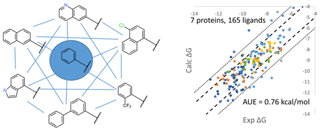
Graphical Abstract

INTRODUCTION

Binding affinity of drug-like molecules to target proteins is a key property that is improved or monitored during the lead optimization stage of small molecule drug discovery. Lead optimization is a time and cost intensive stage,¹ which results from a large number of iterative cycles of design, chemical synthesis and assaying of the compounds. Physics-based modeling methods can bring time and cost savings to lead optimization, by accurately predicting binding affinities of design compounds, because, unlike knowledge based methods², project and chemical series specific training data are not required. Accurate predictions of binding affinities can reduce experimentation by prioritizing compounds likely to result in improved activities. Additionally, a larger chemical space may be explored leading to higher quality compound designs that satisfy multiple property constraints simultaneously.

Explicit solvent based free energy methods offer a full atomistic description of protein-ligand systems within a physically rigorous framework, and thus, have the potential to accurately predict binding affinities. Within this class of methods, alchemical relative free energy methods³ are particularly well suited for lead optimization as they require estimates of relative binding affinities in response to chemical changes to a lead compound. While relative free energy methods are significantly more efficient than absolute free energy methods, the computational cost is still quite high. Contemporary applications of relative free energy perturbation (FEP) calculations typically required 60–390ns of molecular dynamics sampling per ligand screened.^4–6 Because this represents a significant investment in time and resources, there is a strong need to explore and develop methods that can accurately predict binding affinities at a lower computational cost.

Lambda Dynamics (LD), introduced 24 years ago⁷, is an alchemical relative free energy method in which the coupling variable lambda is treated as a dynamic variable with a fictitious mass that is coupled to the system dynamics. In contrast to FEP or Thermodynamic Integration (TI), where a predetermined finite set of lambda values is sampled in multiple simulations, LD implements transformations between thermodynamic end states in a single simulation, with lambda evolution being driven by the intrinsic free energy landscape. A simple probability-based estimator is used to predict the free energy differences. Multiple ligands can be included, which for the problem of protein-ligand binding allows for the calculation of relative binding affinities of multiple ligands in a single LD simulation.^{8, 9} To ensure efficient sampling of all end states, biasing potentials were initially introduced, which are subtracted during post-processing to recover the true free energy differences. Over the years, the method has undergone enhancements including the extension of LD to multi-site lambda dynamics (MSLD)¹⁰ allowing for modeling substituents at distinct sites in a ligand, imposition of implicit constraints that bias the lambda sampling towards the end states¹¹, and biasing potential replica exchange to enhance transitions between them.¹² Importantly, within the last few years developments have been made including the introduction of additional biasing potentials^{13, 14} to flatten the free energy landscape of alchemical transformations, and a soft-core potential¹³, which addressed prior limitations concerning sampling near end states. Another important methodological development involved an algorithm to optimize biasing potentials to promote free energy landscape flattening^{13, 14} which has been applied in recent retrospective studies.^{15, 16}

The above-described developments in LD have set the stage for the application of this method in small molecule lead optimization. However, the following significant impediments exist in way of application to fast paced lead optimization projects. First, screening of multiple ligands in a single LD or MSLD simulation requires preparing a multi-topology ligand that models a shared common core, and separate substituents. Such a multi-topology system is difficult to prepare and prone to errors when setup manually, even more so than for dual topology FEP systems. Secondly, while the Adaptive Landscape Flattening (ALF) algorithm provides an automated way to tune parameters in the biasing potentials used in MSLD, the simulation lengths used in its iterations, and other specifics of the algorithm have not been widely tested. Since the parameters in the biasing potentials need to be refined for each system, the protocol needs to be optimized by testing on a wide variety of protein-ligand systems to ensure effective flattening, and to identify minimal simulation lengths for obtaining accurate results. Finally, other system setup requirements including partial charges, force-field parameter assignment for the ligands and protein, assignment of initial coordinates for the ligands, and generation of solvated simulation systems also need to be reached for MSLD calculations, as with FEP calculations. This paper is aimed at addressing these needs by developing an automated workflow for setting up and executing MSLD calculations, and retrospectively validating it.

The automated MSLD workflow implemented in BIOVIA Discovery Studio and Pipeline Pilot packages¹⁷ is described in detail in the Methods section. Given a core ligand, multiple sites of modification, and the specification of modifications or substituents, the workflow provides tools to setup and execute the MSLD calculations to estimate the binding free energies of a full combinatorial library. A related consideration in lead optimization in addition to screening efficiency is coverage of a broad chemical space in relation to the lead modifications. Keeping this consideration in mind, the MSLD workflow was designed to support the modeling of chemical modifications, which include not only substituents (hydrogen atom replacements), but more broadly, arbitrary modifications as shown in Figures 1–8. The validation dataset was chosen appropriately to represent both small and large lead modifications on a common core. Validation results suggest that the presented MSLD workflow can accurately calculate binding affinities of large combinatorial libraries with significantly greater efficiency than FEP, and thus be of utility in rapidly exploring chemical space to optimize binding affinity, or monitoring it while other drug-like properties are optimized in concert.

Figure 1.

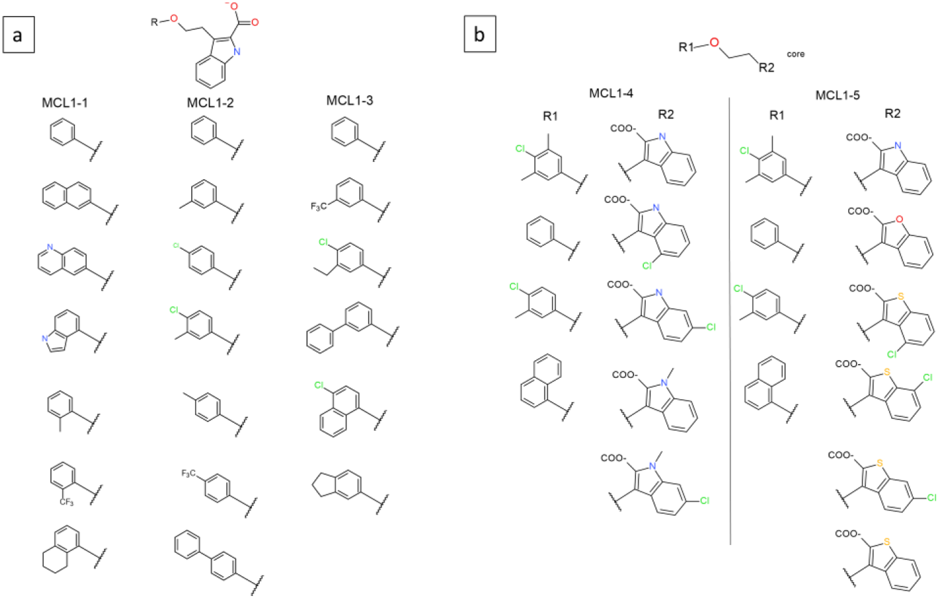
Five MSLD systems used to model ligands in the MCL1 dataset. Panel a shows systems MCL1–1, MCL1–2, and MCL1–3. Panel b shows the two site systems MCL1–4 and MCL1–5. The core ligand is shown on top.

Figure 8.

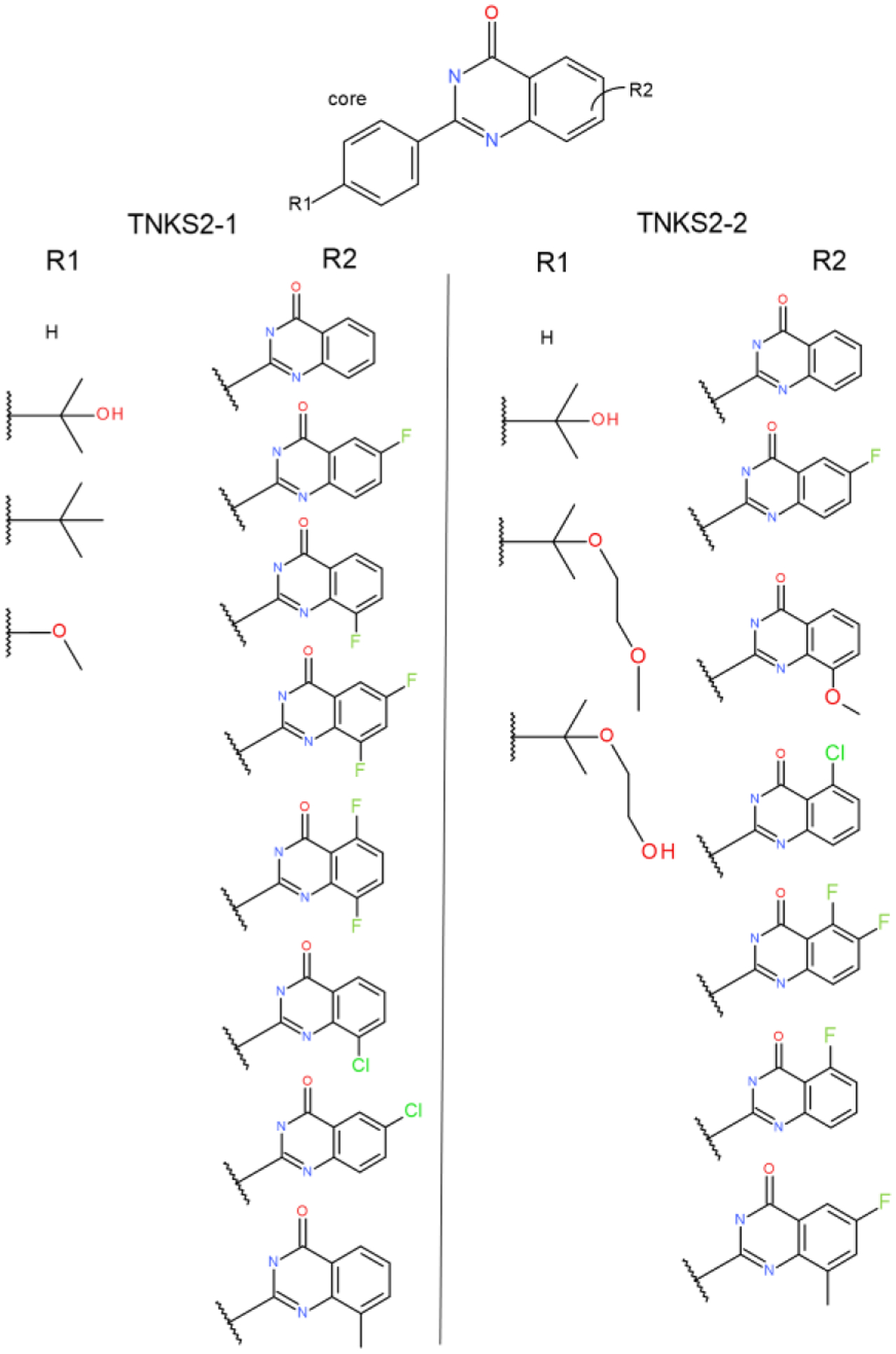
Two MSLD systems used to model ligands in the TNKS2 dataset. Panel a shows the TMKS2–1 system with two sites. Panel b shows the TNKS-2 system also with two sites. The core ligand is shown on top.

METHODS

Lambda Dynamics.

The λ-dynamics methodology has been described in detail in previous works.^{7, 8} Briefly, in contrast with FEP and TI calculations, λ is treated as a dynamic variable. The dynamics of the system is generated using an extended Hamiltonian:

$$H_{\mathit{\text{extended}}}\left(X,\left\{\lambda \right\},\left\{x\right\}\right)=T_x+T_{\lambda }+V\left(X,\left\{\lambda \right\},\left\{x\right\}\right)+V_{\mathit{\text{bias}}}\left(\left\{\lambda \right\}\right)$$

where T_x and T_λ represent the kinetic energies of the atomic coordinates and λ variables. Because λ is treated as a dynamic variable, all intermediate states may be sampled during a single simulation. The third term represents the hybrid potential energy function for the solvent, the protein if present, and the alchemical ligand, and the fourth term is a bias described later. For a single perturbation site with a total of N ligands the hybrid potential term is given by:

$$V\left(X,\left\{\lambda \right\},\left\{x\right\}\right)=\sum _{i=1}^N{\lambda }_{i}V\left(X,x_{S,i}\right)+V_{env}\left(X\right)$$

where X and x_i are the coordinates of the environment and ligand core atoms and of the ligand substituent atoms, respectively, as described below. λ_i is the coupling parameter associated with ligand i. Multi-site lambda dynamics (MSLD)¹⁰ was developed to enable the use of multiple substituents at multiple sites, and the hybrid potential energy function was extended.

$$V\left(X,\left\{\lambda \right\},\left\{x\right\}\right)=V_{env}\left(X\right)+\sum _{S=1}^{M_{\mathit{\text{sites}}}}\sum _{i=1}^{N_S}{\lambda }_{S,i}V\left(X,x_{S,i}\right)+ \sum _{S=1}^{M_{\mathit{\text{sites}}}-1}\sum _{i=1}^{N_S}\sum _{T=S+1}^{M_{\mathit{\text{sites}}}}\sum _{j=1}^{N_T}{\lambda }_{S,i}{\lambda }_{T,j}\left(V\left(x_{S,i}{x}_{T,j}\right)\right)$$

M_sites is the total number of sites that contain multiple substituents, while N_S is the number of substituents at site S off the common ligand core. The double summation in the second term accounts for the interactions between the environment and each substituent at each site. The third term accounts for interactions between each substituent and the substituents modeled at all other sites. However, it is important to note that at a given site substituents do not interact or “see” one another during the simulations. For single site λ-dynamics, a ligand is dominant when its λ value is greater than λ_cut = 0.99. For MSLD, a ligand is described as dominant when the λ values associated with its constituent substituents are all dominant at the same time. Within MSLD, constraints are maintained at each site α according to

$$0\le {\lambda }_{\alpha ,i}\le 1 and\sum _{i=1}^{N_a}{\lambda }_{\alpha ,i}=1$$

To satisfy these constraints, we use an implicit constraint approach¹¹, and simply define λ’s for the N substituents at site α to be:

$${\lambda }_{\alpha ,i}=e^{5.5\text{ sin }{\theta }_{\alpha ,i}}/ \sum _{j=1}^{N_a}{e}^{5.5\text{ sin }{\theta }_{\alpha ,j}}$$

Therefore, for MSLD it is values of θ that have fictious masses, m_θ, and velocities, $\dot{\theta }$, and are propagated through the equation of motion and are transformed back to their corresponding λ values used in free energy determination. The alchemical kinetic energy term is thus defined as

$$T_{\lambda }=\sum _{S=1}^{M_{\mathit{\text{sites}}}}\sum _{i=1}^{N_S}\frac{1}{2}{m}_{\theta }{\dot{\theta }}^2$$

Protein structure preparation.

Protein structures corresponding to the congeneric ligand sets were downloaded from the Protein Data Bank (PDB).¹⁸ Only one protein structure per congeneric set was used as listed in Table 1. Protein structures were prepared using the “Prepare Protein” protocol in BIOVIA Discovery Studio. The p38 MAP kinase protein structure involved two residues with missing coordinates, which were automatically built by the protocol. The protein preparation protocol involves Generalized Born electrostatics based assignment of protonation states consistent with a pH of 7.4, assuming a protein dielectric constant of 10 and ionic strength of 0.145 M, as detailed previously.¹⁹ Any water molecules present in the crystal structures were retained. The CHARMM36²⁰ force-field was used to model the proteins.

Table 1.

Dataset used for retrospective validation. The protein target, PDB ID of the protein structure used, the number of ligands, and experimental affinity range of each set are listed. Also listed are the prediction accuracy metrics from the calculations presented here, the average unsigned error (AUE), root mean square error (RMSE), and correlation coefficient (R) for each set. Units of range, AUE, and RMSE are kcal/mol.

Protein	PDB ID	nLigands	Range	AUE	RMSE	R
MCL1a	4HW3	39	4.19	0.93	1.19	0.73
FAAHb	6MRG	32	5.30	0.70	0.87	0.80
HSP90c	4YKR	16	4.50	0.82	1.18	0.83
PTP1Ba	2QBS	15	2.78	0.39	0.48	0.84
P38MKa	3FLY	27	3.80	0.75	1.07	0.71
CDK2a	1H1Q	16	4.21	0.65	0.79	0.78
TNKS2d	4UI5	20	4.13	0.86	1.09	0.43

Data source:

^a)Wang et al.⁴

^b)Saha et al.³¹

^c)D3R³²

^d)Schindler et al.³³

Ligand preparation and binding pose generation.

Ligands obtained from various sources were either in SMILES format or were converted to the same. Ionization states of ligands were retained as existing in the publication or data source except for HSP90 ligands, where they were manually inspected. For the HSP90 set, a “rule based” method was used to assign a single ionization state for the ligands, following which 2D coordinates were generated. The 3D geometry or binding pose for the congeneric series of ligands in each dataset was assigned using the recently validated “Generate Analog Conformations” (GAC) method.²¹ This method uses the experimental structure of the protein in complex with one ligand in the series as a template, which in this study happens to be the PDB structure listed in Table 1. The method detects the Maximal Common Substructure (MCS)²² between the template ligand and other ligands in the dataset, from which it ascertains the common set of atoms, and atoms that are different. For each ligand, it then directly assigns coordinates for the common set of atoms from the template ligand. For the remaining atoms, a restricted conformational generation procedure is implemented that generates multiple conformations. These conformations are scored using the MM-GBSA method²³ as a first step, and then the protein-ligand complex is energy minimized with non-local (>3 Å away) protein residues held rigid. Following the minimization, a single point MM-GBSA energy calculation is performed to calculate a binding score, which is used to rank the different geometries. The top scoring geometry is selected for the MSLD calculation setup. The Generalized Born Molecular Volume (GBMV) method was used to calculate the solvation energy contribution, which used dielectric constants of 1 and 80, for the solute and solvent respectively. In addition, a linear solvent accessible surface area (SASA) term with slope (α) of 0.00542 kcal mol⁻¹ Å⁻² and intercept (β) of 0.92 kcal mol⁻¹ was included. Further details of the GAC method are available in our previously published study.²¹ Force-field parameters and partial charges for ligands were assigned consistent with CGenFF²⁴ using the MATCH algorithm²⁵ included in Discovery Studio and Pipeline Pilot. For HSP90, P38MK, CDK2, and TNKS2 set ligands, a new atom-typer implemented in the developmental version of the software was used.

Multi-topology builder and simulation system setup.

A MSLD topology builder was implemented that takes as input one core ligand, and multiple additional ligands, each representing a different substituent corresponding to a modification at one of the sites. Each non-core ligand is expected to model one chemical modification with respect to the core at a single site only, and carries a property designating the identity (index) of that site. Ligands corresponding to each site are grouped together, and for each group belonging to a site, a Maximal Common Substructure (MCS) is calculated with the core ligand. Details of the MCS algorithm are described elsewhere.²² When multiple MCS solutions are returned, the one chosen is the one that results in the minimum RMSD based on the positions of the constituent atoms in the ligands. Hydrogen atoms are not considered in MCS computation for algorithmic efficiency, and are subsequently added to the MCS based on the mapping of the parent heavy atoms. The resultant MCS is further reduced by removing atoms that have different force-field atom types and/or partial charge assignment. Hydrogen atoms attached to heavy atoms identified during this step are also removed. In this way, an atom-atom mapping is obtained between the core ligand and all ligands representing a substituent at one site. This process is repeated for all M sites separately, resulting in M MCS solutions. Following this, an intersection of the M MCS is calculated which results in a single MCS. The MCS contains an atom-atom mapping, which encodes the identities of the common core atoms, and atoms that belong to different substituents at different sites. A multi-topology hybrid molecule is created which contains a single copy of the core atoms, and one copy of atoms for each substituent in the different sites. The force-field atom types, partial charges, coordinates, bond connectivity, and improper dihedral definitions for the hybrid molecule are copied from the constituent ligands. Care is taken to not duplicate the bond and improper dihedral definitions involving MCS atoms. Following the creation of the multi-topology ligand, the ligand is solvated in a water box, and a copy is merged with the protein structure and solvated. The solvation step includes neutralizing Na⁺ and Cl⁻ ions consistent with an ionic strength of 0.145 M. Cubic boxes are used to encapsulate the protein-ligand complex and the free ligand systems and ensure at least 7Å between the extremities of the solute and the edge of the box. Two solvated systems are used in MSLD calculations. For a few protein-ligand complex systems simulated in this study, orthorhombic boxes were used instead of cubic to reduce system size. This setup feature was introduced at a later stage during the development of the method and thus only a few systems were modeled with this approach, which include CDK2 systems and the P38MK-8 system. Proteins that may have an elongated shape, when incorporated in orthorhombic boxes have the potential to rotate during the course of the simulation, and consequently come in contact with its own periodic image. This problem does not exist for cubic systems, due to all edge lengths being the same. When using orthorhombic boxes, weak restraints with a force constant of 0.01 kcal mol⁻¹ Å⁻² were applied to the C-alpha carbon atoms of the protein to restrain the translation and rotation of the protein to avoid interaction with its periodic image. Restraints were not applied to binding site residues automatically chosen based on a 5Å proximity criterion to the ligand. A protocol named “Set Up MSLD Calculations” was implemented in Discovery Studio and Pipeline Pilot that generates the MSLD simulation systems given input ligands. Additionally, a protocol named “Enumerate Ligands for MSLD” was developed that makes it easier to generate input ligands for the above protocol. This protocol requires a core ligand and the identification of the sites of modification, and the R-group attachments in SMARTS format.

Bias Optimization.

MSLD simulations use biasing potentials to facilitate transitions among the substituents at each site. Four biasing potentials are used in this implementation as detailed previously,^{13, 14} namely fixed, quadratic, end, and skew biases.

$$V_{\mathit{\text{bias}}}=V_{\mathit{\text{Fixed}}}+V_{\mathit{\text{Quad}}}+V_{End}+V_{\mathit{\text{Skew}}}$$

The functional forms of the lambda dependent potentials are described below.

$$V_{\mathit{\text{Fixed}}}=\sum _s^M\sum _i^{N_s}{\varphi }_{si}{\lambda }_{si}$$

$$V_{\mathit{\text{Quad}}}=\sum _s^M\sum _i^{N_s}\sum _{j>i}^{N_s}{\psi }_{si,sj}{\lambda }_{si}{\lambda }_{sj}$$

$$V_{End}=\sum _s^M\sum _i^{N_s}\sum _{j\ne i}^{N_s}{\omega }_{si,sj}{\lambda }_{si}{\lambda }_{sj}/\left({\lambda }_{si}+\alpha \right)$$

$$V_{\mathit{\text{Skew}}}=\sum _s^M\sum _i^{N_s}\sum _{j\ne i}^{N_s}{\chi }_{si,sj}{\lambda }_{sj}\left(1-\text{exp}\left(-{\lambda }_{si}/\sigma \right)\right)$$

where α=0.017, and σ=0.18 were previously optimized to yield good fits to free energy profiles for a variety of systems.^14–16 The set of constants, {ϕ_si}, {ψ_si,sj}, {ω_si,sj}, and {χ_si,sj} are optimized during bias optimization.

The bias optimization algorithm is iterative in nature where short MSLD simulations are run, followed by calculation of free energy landscapes. Three types of landscapes are computed, the first one being a function of a single lambda value, and the remaining two being a function pairs of lambda values. Single lambda landscapes, G(λ_si) are calculated for each substituent on a site. Free energy landscapes corresponding to transitions between a pair of substituents on a site, G(λ_si/(λ_si + λ_sj)) | λ_si + λ_sj > 0.8, are calculated by using data restricted to the lambda space corresponding to transitions between the two substituents. Pairwise landscapes, G(λ_si,λ_sj) are also calculated using unrestricted data for all pairs of substituents on a site. In a multi-topology ligand, there are N_s G(λ_si) landscapes, and N_s (N_s − 1)/2 pairwise landscapes for each site s. G(λ_si), and G(λ_si/(λ_si + λ_sj)) | λ_si + λ_sj > 0.8 landscapes are calculated by binning the lambda values obtained from the trajectory into 400 bins, and G(λ_si,λ_sj) are calculated by binning pairs of lambda values into 20 × 20 bins. Implicit constraints¹¹ are present in LD simulations, which are subtracted from the landscapes to avoid the flattening the entropic barrier of about 3 kcal/mol in the mid-lambda range. The entropic barrier is retained since it is a desirable feature that promotes more sampling in the end states. A running window average of the landscapes is calculated using the most recent six simulations, where thermodynamic averaging is performed using the weighted histogram analysis method (WHAM).¹³

For each landscape, a flatness parameter is calculated as the root mean squared deviation from the F = 0 line, and an average flatness is calculated over all single, and pair lambda landscapes, respectively. For pairs of substituents, the flatness parameter is only calculated for the transition landscapes. Iterations are terminated when the average flatness falls below a specified threshold value. This is done so as to avoid running further simulations if the free energy landscapes are sufficiently flat. However, this termination criterion is only invoked in Phase 1 of the bias optimization protocol (see below). One set of biases is chosen from the last six iterations that provides the most even sampling for all substituents on all sites, which is implemented by maximizing an entropy metric calculated as follows

$$S=\sum _s^M\sum _i^{N_s}-p_{si}\text{ln}{p}_{si}$$

where p_si is the probability of λ_si > λ_cut (and λ_cut = 0.99).

A three phase bias optimization protocol was implemented. The first phase runs 100 iterations of 100ps long MSLD simulations. If the average flatness parameters associated with single and pair (transition) lambda landscapes described above reaches a value below 0.25 and 0.5 kcal/mol, respectively, iterations are terminated. The second phase of bias optimization runs 10 iterations of 1ns long MSLD simulations, and the third phase runs 5 iterations of 2ns long simulations. At the end of each phase, the last six iterations are evaluated, and the biases associated with the simulation that results in the maximum entropy metric are chosen for the next phase or for production simulations.

MSLD production simulations.

All simulations were performed under periodic boundary conditions. The van der Waals (vdW) interactions were switched off smoothly in the range 10−12 Å, and the particle mesh Ewald method^{26, 27} was used to treat long range electrostatics with a real space cut off of 12 Å. An integration time step of 2 fs was used for dynamics. Production simulations were performed in the NPT ensemble, where a temperature of 298.15K was maintained using the Nose-Hoover thermostat method and pressure of 1 atm maintained using the Langevin piston method. A soft-core potential¹³ was used to alleviate end-point singularities. The MD simulation parameters used in the production stage are identical to those used in the bias optimization stage.

Production runs involve six independent trajectories, which are each 20ns long each, for a cumulative sampling time of 120ns. Two series of production runs are performed, one for the free ligand in solvent, and one for the solvated protein-ligand complex. From each trajectory, the free energy of each combinatorial ligand c from trajectory t is calculated as follows

$$F_c^t=-k_{B}T\text{ln}{p}_c^t-V_{\mathit{\text{Fixed}},c}$$

where $p_c^t$ is the probability of all substituents involved in combination c to have their respective lambda values λ_si > λ_cut. V_Fixed,c is the sum of fixed biases corresponding to the substituents in combination c. The fixed bias is subtracted to retrieve the unbiased true free energy. Estimates from trajectories 1–2, 3–4, and 5–6 are combined to obtain three free energy values for each combination c. A Boltzmann average of free energy estimates from two trajectories ti, tj is obtained as follows.

$$F_c^{ti,tj}=-k_{B}T\text{ln}\frac{\text{exp}(-F_c^{ti}/k_{B}T)+\text{exp}(-F_c^{tj}/k_{B}T)}{2}$$

The free energy associated with a combination F_c is calculated as a simple average over $F_c^{t1,t2}$, $F_c^{t3,t4}$, $F_c^{t5,t6}$ values - a corresponding standard deviation is also calculated. Relative binding free energies are calculated by taking of the difference of F_c calculated in the complex and free ligand states. A standard deviation associated with the prediction is calculated as the square root of the sum of squares of the standard deviations associated with complex and free ligand states.

From each MSLD simulation, the time series of lambda values corresponding to each substituent output at a frequency of 0.02 ps was extracted. The lambda time series was transformed into a “state time series” which indicates the identity of a substituent si that is active at a given time point λ_si > λ_cut. The state time series is processed individually for each site. For each substituent si, the number of times the system transitions from any substituent sj to si, or from si to any substituent sj is counted as the number of transitions associated with si. Transition rates are calculated for pairs of trajectories over a total sampling time of 40ns, resulting in three estimates which are averaged to obtain the expected number of transitions over 40ns.

Comparison to experiment and prediction metrics.

Validation included one site and two site systems that modeled 5–32 ligands per system, and two and three site systems that modeled large combinatorial libraries of 64–180 ligands per system. Twenty-five one site and two site systems were created by dividing the seven datasets into smaller subsets. For a given protein, subsets were created so as to maintain a common reference ligand in all sets to enable the calculation of absolute binding affinities by using the experimental affinity of the one reference ligand. The prediction metric used to assess accuracy in the 25 small subsets was average unsigned errors of ΔΔG values with respect to the corresponding experimental values. To observe the overall prediction quality for each protein set, the absolute binding affinity ΔG was calculated by first using the experimental ΔG of one common ligand used as a reference in each subset. Following the approach in other retrospective free energy studies^{4, 5}, a single offset value was added to the calculated ΔG value to minimize errors associated with the choice of a single reference ligand as the lead compound with known affinity. The same approach was followed for the calculation of the AUE of ΔG for the large scale multi-site systems modeled in this study. Other metrics including root mean square error (RMSE), and correlation coefficient (R) were also calculated to assess the quality of predictions for each protein set.

MSLD Workflow.

The MSLD workflow implemented in the Discovery Studio and Pipeline Pilot packages¹⁷ was used to run all calculations. The 2020 release of the software included prototype MSLD functionality that incorporates protocols to setup MSLD systems, run bias optimization, run production, and collate results. In addition, a helper protocol for enumerating R-group features on a core ligand, and another protocol to generate initial binding poses²¹ of ligands are also included. Calculations discussed in this study were run with a developmental version of the software that added a protocol to combine bias optimization, and production to support multi-phase bias optimization, with enhanced efficiency and usability. The MSLD simulations during bias optimization and production stages are run with CHARMm²⁸ included in the software, using the DOMDEC-GPU platform²⁹. These stages can be run on a Pipeline Pilot server installed on a GPU cluster (grid) with a supported queuing system to allow for automatic queuing and execution.

RESULTS

To evaluate the accuracy and reliability of the MSLD workflow, it was tested on a diverse dataset, which is described below. All steps of the workflow are implemented in Discovery Studio and Pipeline Pilot packages¹⁷, which include protein preparation, ligand binding pose generation, force-field assignment, MSLD multi-topology setup, MSLD bias optimization, production, and analysis. These steps are described in detail in the Methods section. For each MSLD system prepared, a three phase bias optimization was performed with up to 10ns of simulation time in each phase, for a cumulative time of 30ns. The number of iterations and iteration length in the three phases were 100 × 100ps, 10 × 1ns, and 5 × 2ns, respectively. Phase 1 is initiated with all biases set to zero, and short iterations run adaptively adjust the biases more frequently. In later phases 2 and 3, which are initiated with biases optimized in prior phases, longer iterations are helpful to obtain more sampling allowing more refined adjustment to the biases. With the optimized biases, six independent trajectories of 20ns long production simulations are run, which are merged to generate three trajectory segments representing 40ns of sampling each. A combined estimate of the average free energy and standard deviation is obtained from the production simulations (see Methods). We note that on average, the statistical precision of each prediction was +/− 0.48 kcal/mol, suggesting our proposed protocol with the sampling regimen noted above are of sufficient precision for prioritizing compounds in lead optimization.

Datasets.

The validation dataset was collected from publicly available congeneric ligand sets with experimentally measured binding affinities and a co-crystal structure of the protein in complex with one of the ligands, or a similar ligand in the PDB.¹⁸ Additionally, the choice of the datasets and ligands within each was motivated by the desire to validate the presented method for its domain of applicability, which is to efficiently screen multiple modifications to a common core compound at single or multiple sites. Seven congeneric sets were collected from various sources as listed in Table 1. Since most datasets that we found were originally collated to validate FEP approaches, a subset of ligands from each was selected that fit the domain of applicability. A few ligands from each set could not be included because those involved modifications at many different parts of the core and were outside the focus of our current study. Another consideration for selecting the ligands used for validation arose from prior MSLD studies that have found efficient sampling among substituents that were similar in shape or volume.¹² While this consideration was taken into account, the selected ligands were also chosen to model chemically and structurally diverse substituents (Figures 1–8). The range of affinities for most sets is around 4 kcal/mol (Table 1), which represents a 1000-fold change in binding affinity, and thus provides an opportunity to test the method’s ability to capture large changes in affinity. Four of the seven sets provided an opportunity to test multi-site substitutions, which included the proteins MCL1, HSP90, P38 MAP kinase (P38MK), and TNKS2. TNKS2 ligands involving a change in net charge (8 series) were not included. Net charge changes among the ligand series could potentially be modeled accurately in MSLD by applying end-point corrections as done in the context of FEP³⁰. However, this straightforward application of MSLD was not the focus of the present study. Thirty two ligands from the “left-side” group in Ref³¹ were included from the FAAH dataset. Most of the “right-side” ligands involved experimental measurements from racemic mixtures, and thus this set was not included in our study. A subset of ligands from the HSP90 dataset from D3R was selected that could be modeled with substituents on two sites. A complete list of ligands examined in the study can be found in the data included in the Supporting Information files, which includes the ligand and protein structures used to initiate the MSLD calculations.

MSLD calculations on diverse subsets.

The seven datasets described above were divided into subsets that differed in number of sites, number of substituents, and chemical and topological diversity of the substituents (Table 2). This was done to evaluate the MSLD workflow to accurately calculate the relative binding free energies under different scenarios. For example, the efficient and reliable sampling of diverse substituents within a single series represents a stringent test of our MSLD workflow implementation. In addition to the differences in ligands, the nature of the protein pocket may also influence sampling and transition rates between different bound states. Thus, twenty five datasets listed in Table 2 were constructed to test the protocol adopted in the bias optimization and production stages. Overall, the subsets model 5 to 32 ligands each using either one or two sites, as shown in the figures below. The 25 subsets categorized by the protein target are discussed below.

Table 2.

Subsets representing MSLD systems modeled to cover each validation set. The subset ID, number of sites (N Sites), number of substituents (N Subs), number of ligands with experimental data (N Exp), experimental affinity range (Range), and average unsigned error (AUE) obtained for each system are listed. Average and standard deviation of AUE is also listed. Units of Range and AUE are kcal/mol.

Subset ID	N Sites	N Subs	N Exp	Range	AUE
MCL1–1	1	7	7	3.18	0.87
MCL1–2	1	7	7	2.70	0.73
MCL1–3	1	6	6	2.56	1.11
MCL1–4	2	4×5	13	3.85	0.92
MCL1–5	2	4×6	14	3.38	1.16
FAAH-1	1	8	8	4.50	0.92
FAAH-2	1	8	8	4.28	1.00
FAAH-3	1	8	8	4.47	0.78
FAAH-4	1	6	6	2.06	0.74
FAAH-5	1	6	6	1.68	0.63
HSP90–1	2	6 × 5	9	4.30	1.04
HSP90–2	2	8 × 2	9	4.51	1.15
PTP1B-1	1	6	6	1.27	0.55
PTP1B-2	1	6	6	1.74	0.22
PTP1B-3	1	5	5	1.36	0.52
P38MK-1	1	5	5	2.40	0.90
P38MK-2	1	5	5	1.40	1.15
P38MK-3	1	5	5	1.21	0.68
P38MK-4	1	7	7	2.45	1.50
P38MK-5	1	5	5	1.71	1.00
P38MK-6	1	5	5	1.36	1.39
CDK2–1	1	9	9	2.74	0.69
CDK2–2	1	8	8	3.42	0.80
TNKS2–1	2	4×8	12	3.53	1.16
TNKS2–2	2	4×7	11	4.13	1.12
				Average	0.91
				Std. Dev.	0.29

MCL1 dataset:

39 ligands included from this dataset were modeled as 5 MSLD systems or subsets which are listed in Table 2. Figures 1a and b illustrate the ligands modeled in this dataset. Systems MCL1–1 to 3 shown in Figure 1a involve single site representatives and systems MCL1–4 and 5 shown in Figure 1b are modeled with two sites each. Systems MCL1–1, 2, 3 include 7, 7, and 6 substituents, respectively, and collectively model 18 different aromatic R-groups. The aromatic groups modeled in each system are quite diverse, as a result of which the number of additional heavy atoms in each substituent compared to the common core are 3–7, 3–9, and 4–10 heavy atoms in systems MCL1–1, 2, and 3, respectively. The MSLD simulations involve transitions between the different substituents and thus model changes involving an even larger number heavy atoms. For example, in MCL1–1 system, a transition from substituent 2 to 3 involves a change in 14 heavy atoms, 7 from substituent 2 (disappearing), and 7 from substituent 3 (appearing). The low AUE obtained for these subsets (Table 2) illustrates the ability of the developed workflow to sample large and diverse groups.

Figure 1b shows two-site systems MCL1–4 and MCL1–5, which involved 4×5, and 4×6 substituents, respectively. While the two two-site systems modeled 20 and 24 systems, respectively, only 13/20 and 14/24 substituent combinations had experimental data associated with them. The four substituents involved in Site 1 in both these systems are the same. In system MCL1–4, site 2 groups differ in the placement of the chloro and methyl groups, whereas in MCL1–5, the carboxylic acid group involves more diverse chemistry that includes indole, benzofuran, and benzothiophene groups. In MCL1–4, 7 out of the 12 heavy atoms of the heterocyclic carboxylic acid group are included in the MCS, whereas for MCL1–5, due to the diversity of substituents in site 2, only 4 out of 12 heavy atoms are in the MCS. The MCL1–5 system exemplifies the ability of the method to model chemically diverse groups to a greater degree than MCL1–4.

To further examine the efficiency of the landscape flattening we monitored the number if transitions involving each substituent in all 25 subsets, for a total of 185 substituents, this is shown in Figure S1 of the Supporting Information. The first 39 data points correspond to the substituents modeled in systems MCL1–1 to 5. Each point is an average over number of transitions calculated in the three 40ns trajectory segments. The length of each arm of the error bar equals the standard deviation over the three values. A general observation is that the number of transitions in the protein-ligand complex state are lower than in the free ligand state. However, for most substituents the number of transitions in both states is high. For the MCL1 systems, the number of transitions per 40ns trajectory segment per substituent range from an average of 220 to 3541 in the complex state and even higher in the free ligand state. Thus, the data strongly suggest that all substituents are sampled well.

Ligand 27 was common to all the MCL1 subsets, based on which the absolute binding affinities of the entire congeneric set could be calculated from the relative values obtained from each subset. Figure 2a displays the calculated vs. experimental absolute binding free energies, ΔG_b for the MCL1 set. Error bars depict the associated standard deviation.

Figure 2.

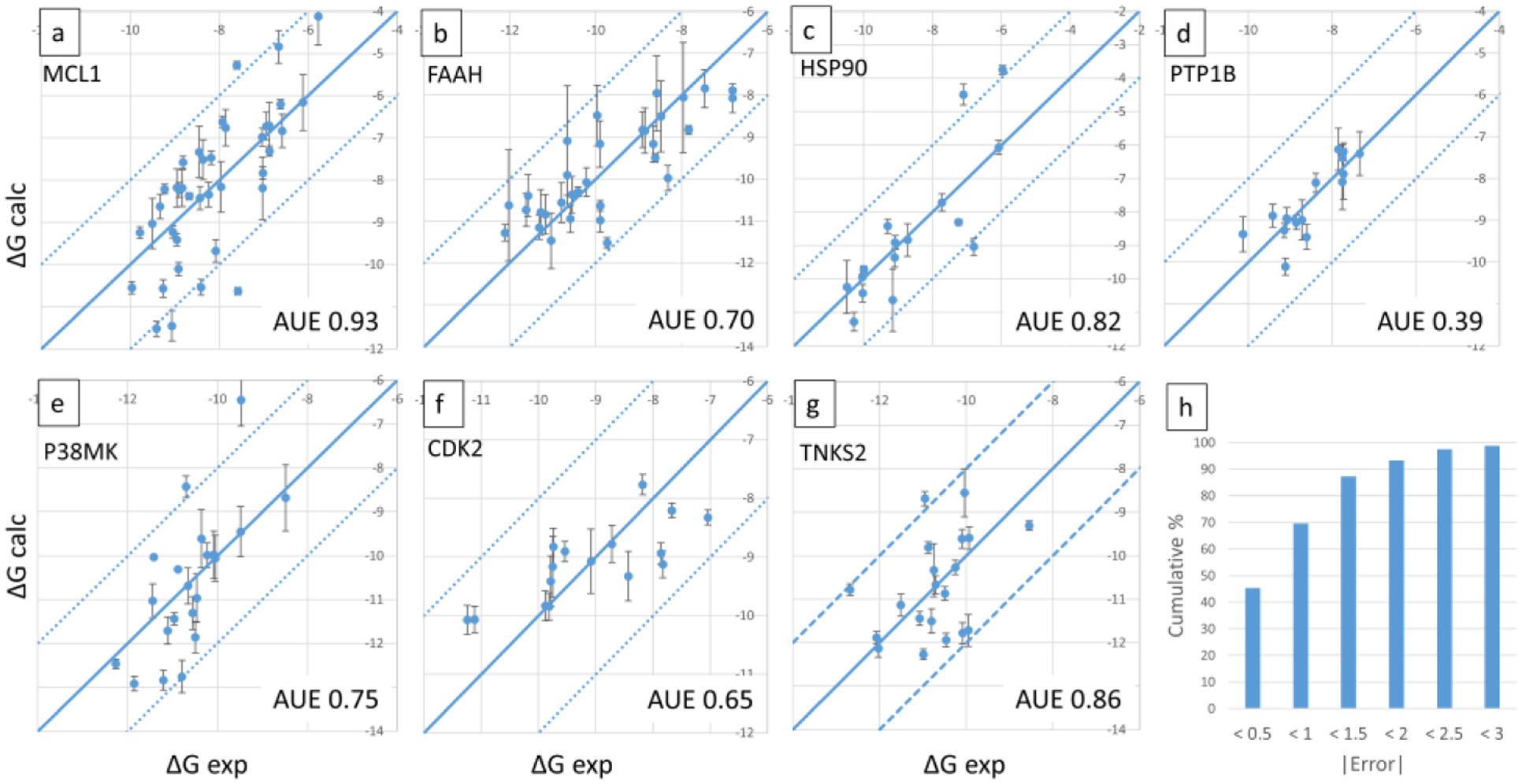
Calculated vs. experimental absolute binding free energies for the seven datasets are shown in panels a-g, with the name of the protein indicated on top left, and AUE on bottom right. Panel h shows the cumulative percentage of ligands for which absolute errors in predictions are lesser than different error bounds. Calculated relative free energies were converted to absolute by adding a constant offset value that minimizes errors associated with the choice of a single reference ligand as described in Methods. Units are kcal/mol.

FAAH dataset:

32 inhibitors of the Fatty Acid Amide Hydrolase (FAAH) protein previously modeled in a FEP study³¹ were selected. The 32 ligands were divided into 5 subsets from which single site MSLD ligand systems were created. MSLD systems FAAH-1, 2, and 3 modeled 8 ligands each, whereas FAAH-4 and 5 modeled 6 ligands each. Ligand 31 was included as a reference in each system. Figure 3a (FAAH-1 to 3) and b (FAAH-4 and 5) illustrate the MSLD systems modeled. The ligands present different R-groups in the ortho, meta, and para positions on the “left” phenyl ring³¹ of the core ligand. Ligands in the set involve differences of up to six heavy atoms with respect to the unsubstituted phenyl ring. Table 2 shows the range of experimental affinities in the five subsets to be 1.68 – 4.5 kcal/mol, with the range being greater than 4 kcal/mol for three sets. For 31 of the 32 substituents overall, the average number of transitions per 40ns trajectory segment in the complex state are greater than 70 (Figure S1). The lowest number of transitions were recorded for FAAH-3 sub-2 in the complex state, which models the cyano group at the para position. However, this does not affect the accuracy of the prediction – the unsigned error for this prediction is only 0.14 kcal/mol. For the free ligand state, all substituents involved more than 80 transitions.

Figure 3.

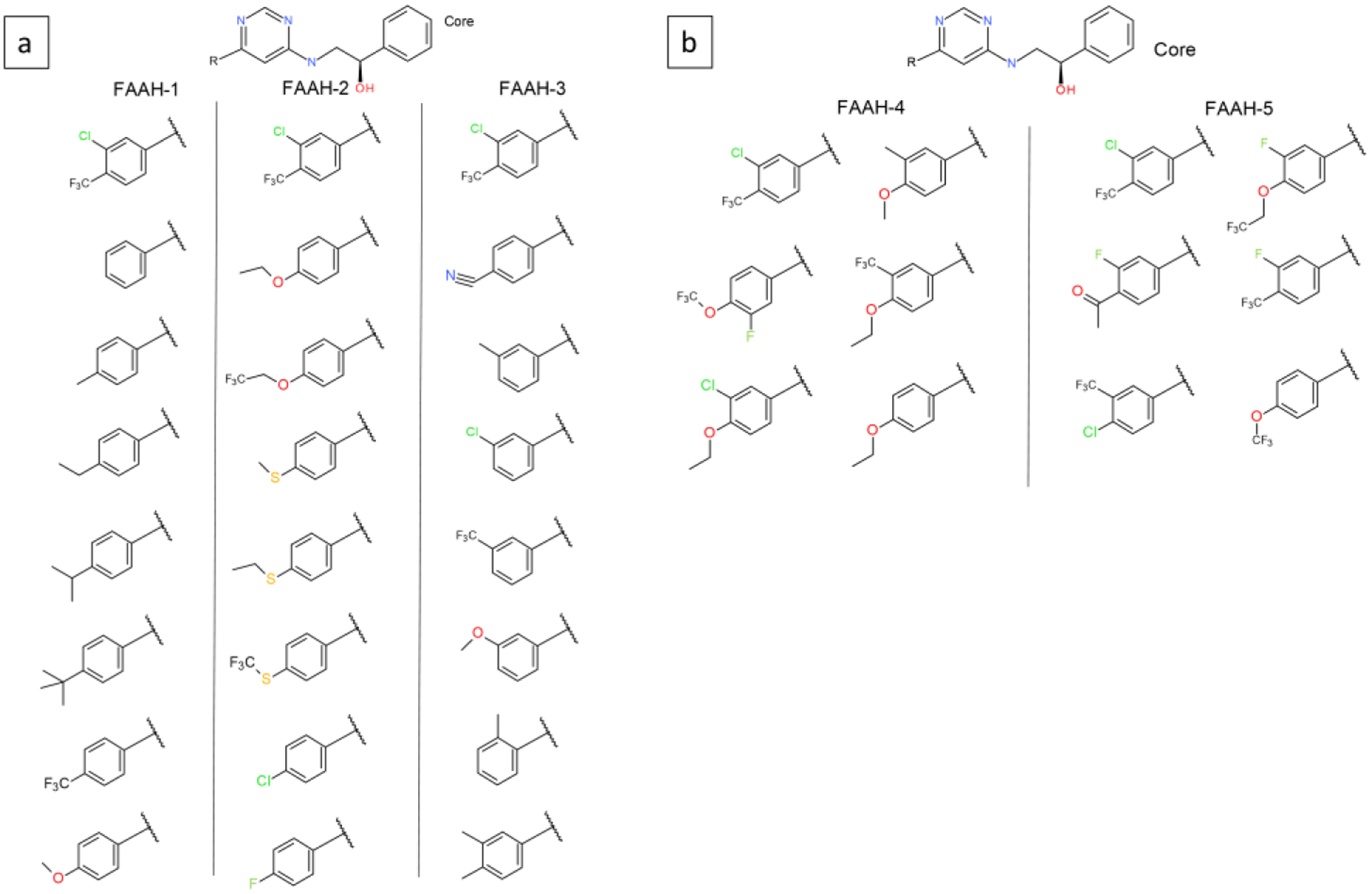
Five MSLD systems used to model ligands in the FAAH dataset. Panel a shows systems FAAH-1, FAAH-2, and FAAH-3, which model eight substituents each. Panel b shows FAAH-4 and FAAH-5, which model six substituents each. The core ligand is shown on top.

The AUE for the 5 subsets range from 0.63 to 1 kcal/mol, which suggests good predictive power for sets spanning a wide range of affinity. Using ligand 31 as a common reference present in all subsets, absolute binding free energies, ΔG_b was calculated for all 32 ligands. Figure 2b illustrates the calculated vs. experimental ΔG_b, with an overall AUE of 0.7 kcal/mol.

Hsp90 dataset:

Two 2-site systems were modeled to include the HSP90 ligands. Figures 4a and b show the two MSLD systems. In HSP90–1, site 1 involves R-group decorations on a phenyl ring, whereas site 2 includes more diverse R-groups. In HSP90–2, site 2 contains only two substituents, but site 1 includes substituents that have significant differences in size, and chemistry. For example, substituent site1-sub8 includes 11 additional heavy atoms compared to sub1. In addition, site 1 is located in a relatively occluded region of the binding pocket (Figure 4b inset), such that the transitions from small substituents (eg. site1-sub1) to large ones such as sub8 shown in the figure would require the protein pocket to open up further (discussed below).

Figure 4.

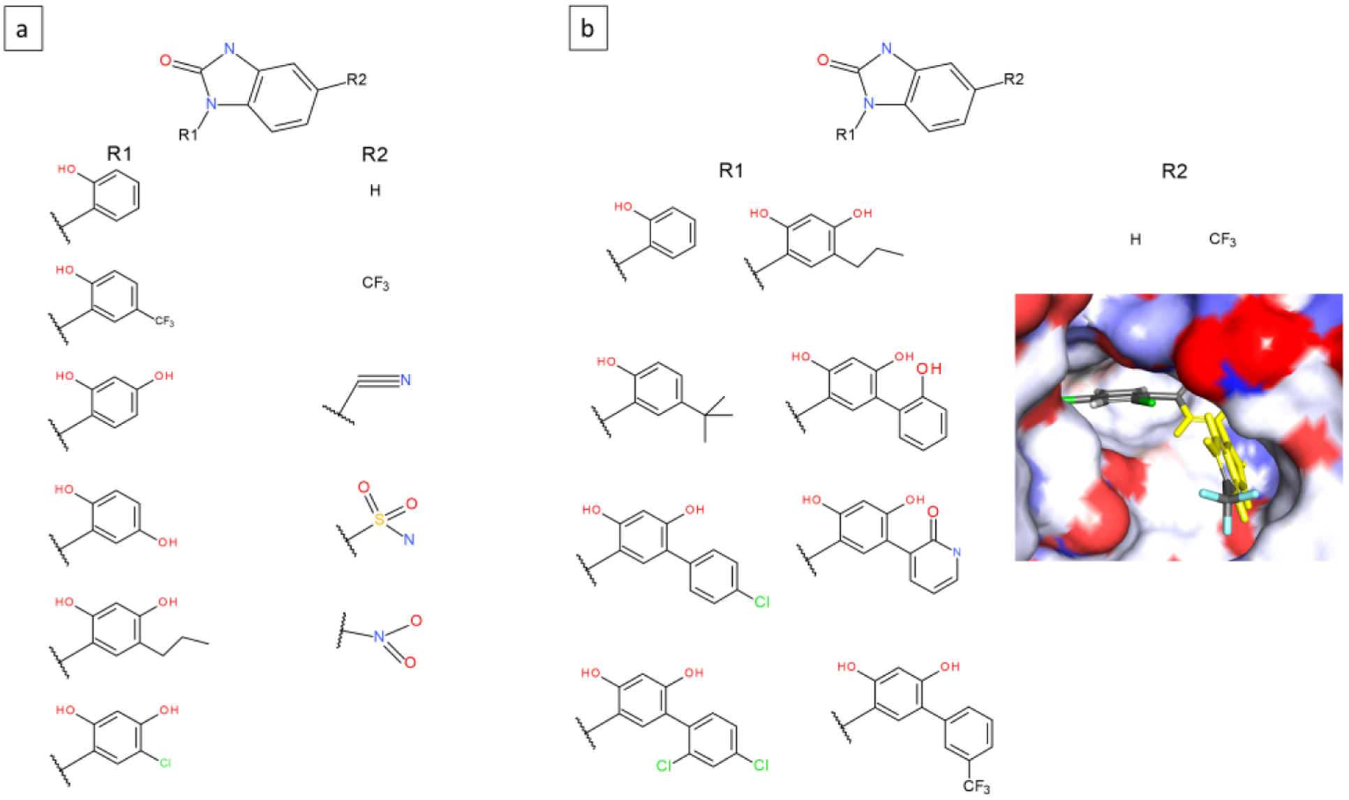
Two MSLD systems used to model ligands in the HSP90 dataset. Panel a shows the HSP90–1 system with two sites. Panel b shows the HSP90–2 system also with two sites. Inset shows the partly occluded binding pocket near site 1. The core ligand is shown on top.

Since the two MSLD systems model 6×5 and 8×2 substituents, 30 and 16 free energy values, respectively, are calculated from the simulations, out of which experimental data exists for 9 combinations in each set. The AUE obtained for the two sets with ranges of 4.3 and 4.51 kcal/mol, are 1.04 and 1.15 kcal/mol, respectively. The slightly higher error for HSP90–2 system is consistent with the larger size differences among the 8 substituents in site 1. This is reflected in the number of transitions observed for the substituents in the complex state. While substituents 4–8 record more than 40 average transitions are relatively low at 5.3, 14, and 4.3 for substituents 1, 2, 3, respectively (Figure S1). The absolute error in predicted ΔG for the ligands that correspond to site1-sub1 and site1-sub3 are high at 2.22 and 2.24 kcal/mol, respectively, which appears consistent with the low number of transitions.

Figure 2c illustrates the calculated vs. experimental absolute binding free energies, ΔG_b for 16 ligands which represent the combinations of substituents for which experimental affinities were available. The AUE for this dataset is 0.82 kcal/mol.

PTP1B dataset:

Three single site MSLD systems were constructed to model ligands from the PTP1B dataset with 6, 6, and 5 substituents, respectively, shown in Figure 5. Substituents in all three groups of ligands are not only chemically but also topologically diverse. While Table 2 shows the AUE obtained for the three sets is very low, the experimental binding affinity ranges of the individual sets at 1.27 – 1.74 kcal/mol is relatively small. However, the accurate results obtained for the set of ligands with R-groups that have significant topological differences shows the power of the method in exploring chemical space broadly. Except for one substituent with 81 average transitions, all have more than 150 in the complex state. The number of transitions in the free ligand state are much higher (Figure S1). Figure 2d plots the calculated vs. experimental ΔG_b for the 15 ligands in this dataset, with an AUE of 0.39 kcal/mol.

Figure 5.

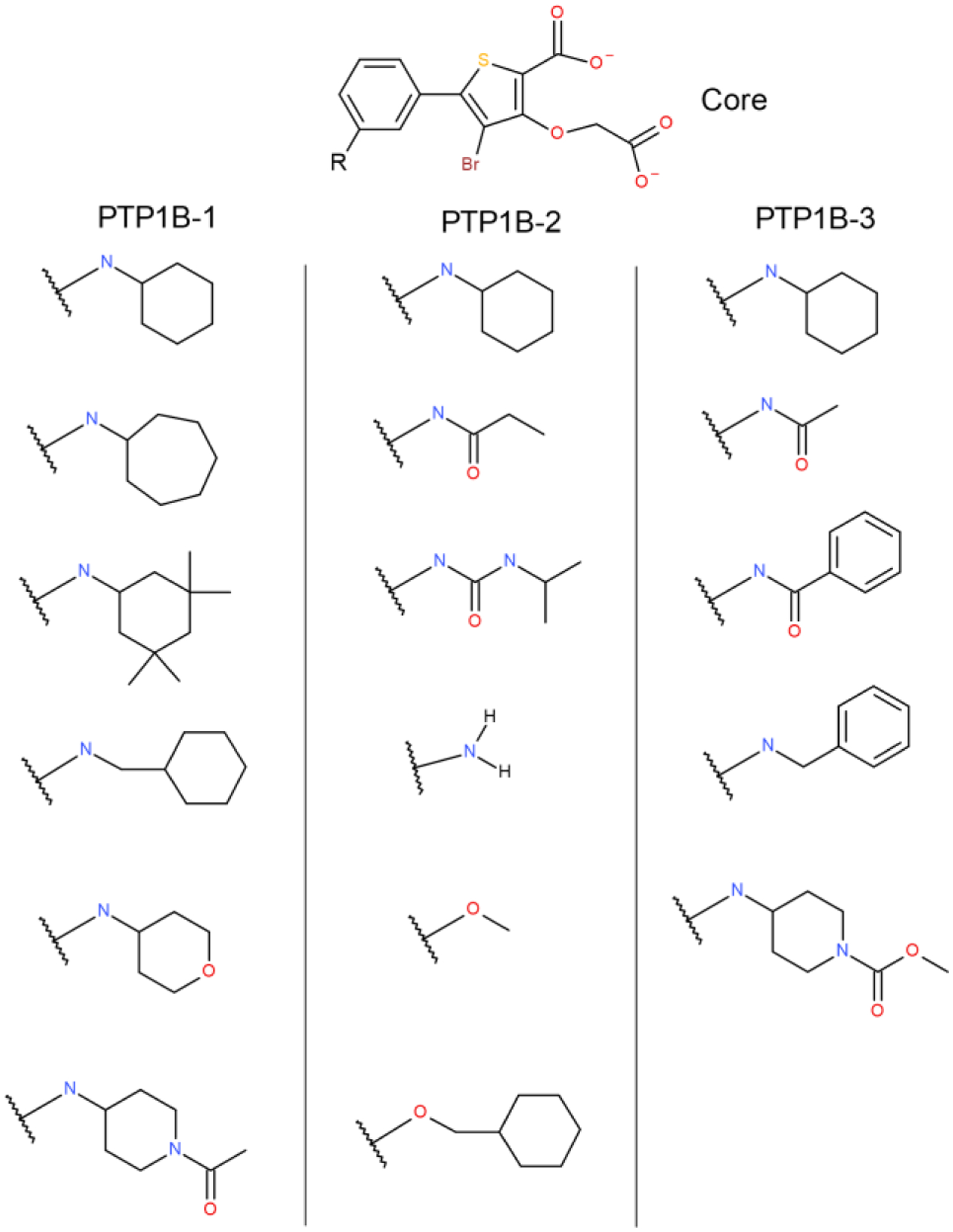
Three MSLD systems used to model ligands in the PTP1B dataset. The core ligand is shown on top.

P38 MAP kinase (P38MK) dataset:

The 27 ligands from the P38MK set were modeled by dividing them into 6 subsets, which are shown in Figure 6a–c. This dataset includes three sites of modifications. The first site is modeled by systems P38MK-1 and 2, the second site is modeled using P38MK-3 and 4, and the third one using P38MK-5 and 6. The P38MK-1 system models relatively small modifications that involve fluorine substitutions on the phenyl ring. In the P38MK-2 system on the other hand the linker atom is different or absent (sub 4) resulting in this set being very diverse. Similarly, P38MK-3 to 6 also model groups that are diverse both chemically and topologically. All 32 substituents modeled across the six systems recorded greater than an average of 50 transitions per 40ns trajectory segment, except for one with 37, indicating sufficiently sampled substituents. Table 2 shows the AUE obtained for each site. P38MK-4 has a relatively high AUE of 1.5 kcal/mol, but for the remaining P38MK sets it is similar to other ligand series evaluated in this study. ΔG_b for all the 27 ligands were calculated using P38MK-1 sub1 ligand as reference, and are displayed in Figure 2e. An AUE over all ligands is 0.75 kcal/mol.

Figure 6.

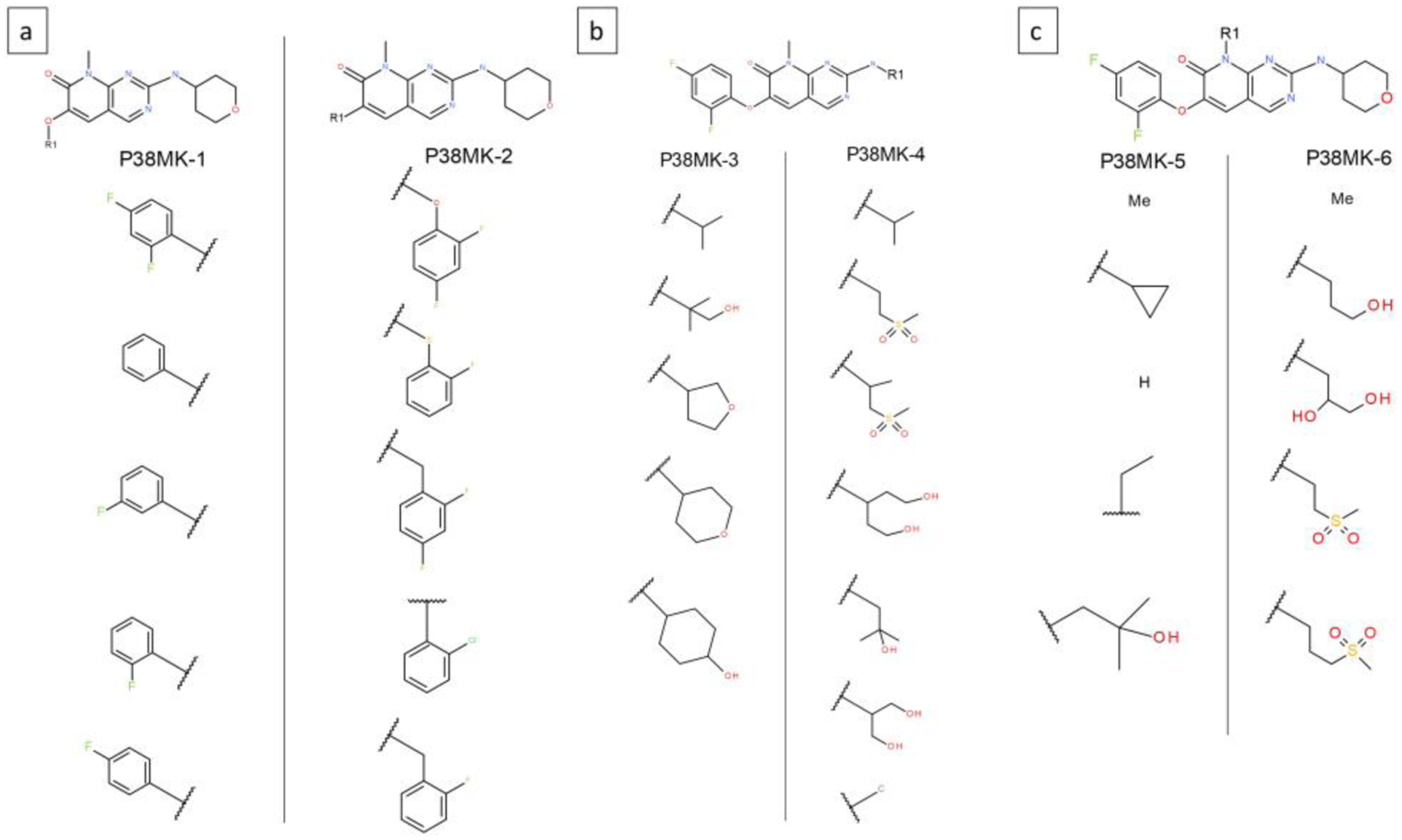
Six MSLD systems used to model ligands in the P38 MAP kinase dataset. Panel a shows systems P38MK-1 and 2. Panel b shows systems P38MK-3 and 4. Panel c shows systems P38MK-5 and 6. The core ligand is shown on top.

CDK2 dataset:

16 ligands from the CDK2 set were modeled using two single site systems, CDK2–1 and CDK2–2, which included 9 and 8 substituents, respectively (Figure 7). The ligands involved differences in R-group substituents on a terminal phenyl ring, on meta or para positions or both. All 17 substituents modeled across the two systems recorded greater than an average of 50 transitions per 40ns trajectory segment, indicating sufficiently converged results (Figure S1). Low values are obtained for the overall AUE for the 16 ligands (Table 1), and for the two sets separately (Table 2). Figure 2f shows the calculated vs. experimental absolute binding free energies.

Figure 7.

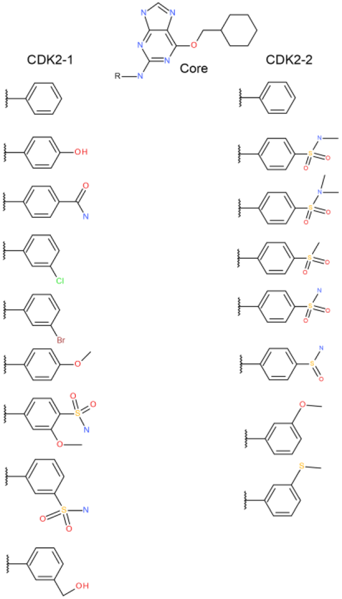
Two MSLD systems used to model ligands in the CDK2 dataset. The core ligand is shown on top.

TNKS2 dataset:

20 ligands from the TNKS2 set were modeled using two two-site MSLD systems depicted in Figure 8. Site 2 in both systems involve substitutions and combinations of fluorine, chlorine, methyl, and methoxy groups on the quinazolinone group. Site 1 in TNKS2–1 system involved small changes, whereas in TNKS2–2 system large flexible alkyl chains were included. All 23 substituents modeled across the two systems recorded greater than an average of 200 transitions per 40ns trajectory segment (Figure S1), indicating sufficiently sampled substituents. The AUE obtained for the two sets is higher than the overall average of the 25 subsets in this study, but the calculated affinities are still predictive. Figure 2g plots the calculated vs. experimental ΔG_b, with an AUE of 0.86 kcal/mol (Table 1).

Screening large combinatorial libraries.

The above described MSLD systems involved one or two sites that incorporated 5 to 32 combinatorial ligands each. Given the multi-site nature of the method, it is of interest to evaluate scaling to larger combinatorial libraries. With this goal in mind, five MSLD systems were created that spanned the same datasets as discussed above. A first and natural choice for a three site MSLD system was the P38MK dataset which includes modifications at three well separated sites on the core ligand. The three-site system P38MK-7 was constructed to include 5×5×5 substituents, which is shown in Figure 9a. Table 3 lists several characteristics and results for the different MSLD systems modeled to predict binding affinities of relatively large combinatorial libraries. For P38MK-7, 122 out of the 125 combinatorial ligands were sampled during the production simulations, predictions for which are displayed in Figure 9b. The ΔΔG values are calculated relative to a reference compound that models substituent 1 on all three sites. About one-third of the ligands are predicted to be as potent as the reference compound based on the error bars overlapping with the ΔΔG=0 line. The remaining compounds exhibit significantly different affinities. This analysis suggests that the calculated affinities of all combinations can help screen for compounds with significantly improved binding affinity. Furthermore, an analysis of the substituents involved in the tightest binding ligands can result in design insights relevant to lead optimization. For example, the top six ligands ranked by favorable affinity include sub4 at site 2, suggesting its importance in binding. The Discussion section below illustrates this by presenting a structural analysis of a ligand with substituent 4 on site 2. Experimental data were available for 13 combinations (red bars in Figure 9b), spanning a range of 3.78 kcal/mol. The AUE obtained for this subset of data was 0.61 kcal/mol. Figure 9c plots the calculated vs. experimental absolute binding free energies, ΔG_b for 13 ligands which represent the combinations of substituents for which experimental affinities were available.

Figure 9.

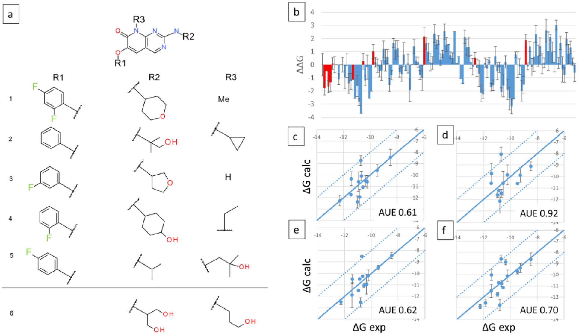
Three site MSLD systems P38MK-7 and P38MK-8. Panel a shows the core ligand with three sites of substitutions, and the corresponding substituents. All substituents involved in P38MK-7 are depicted above the horizontal line. One additional substituent each for site 2 and 3 that are modeled in P38MK-8 are depicted below the line. Panel b displays the calculated ΔΔG values for 122 out of 125 combinatorial ligands modeled in system P38MK-7, with red bars indicating ligands for which experimental data is available. Panels c and d display the calculated vs. experimental absolute binding free energies for P38MK-7 and P38MK-8 sets, respectively. Panels e and f display binding free energies calculated using the additive approximation for P38MK-7 and P38MK-8 sets, respectively. Calculated relative free energies were converted to absolute by adding a constant offset value that minimizes errors associated with the choice of a single reference ligand as described in Methods. AUE are indicated on bottom right. Units are kcal/mol.

Table 3.

MSLD systems representing large scale combinatorial screening. The Subset ID, number of sites (N Sites), fraction of ligands sampled (N Sampled), number of ligands with experimental data that were sampled (N Exp), experimental affinity range and average unsigned error (AUE) obtained for each system are listed. For N Exp, the number in parentheses if present indicates the number of ligands with experimental affinity sampled in the MSLD simulations. Units of range and AUE are kcal/mol.

Subset	N Sites	N Sampled	N Exp	Range	AUE	AUE (additive)
P38MK-7	5 × 5 × 5	122/125	13	3.78	0.61	0.62
P38MK-8	5 × 6 × 6	131/180	15 (12)	2.96	0.92	0.70
MCL1–6	7 × 4 × 4	109/112	16 (14)	4.19	0.84	0.67
MCL1–7	8 × 8	58/64	23 (21)	3.85	1.11	0.90
HSP90–3	6 × 5 × 3	68/90	9 (5)	1.19	0.39	0.43

To monitor the extent of scalability, a second system, P38MK-8, with the same substituents as in P38MK-7, but with a sixth extra substituent each for sites 2 and 3 was also constructed (5×6×6 substituents; Figure 9a). For this system, 131/180 ligands were sampled, which suggests that for this system and substituent combination, 180 ligands represent an upper limit of the combinations that can be visited during 120ns of cumulative sampling. Out of the 49 ligands that were not sampled, 31 ligands involved only substituents 1–5 on all sites. Since nearly all ligands involving these substituents were sampled in P38MK-7 system, the reason for the lesser number of sampled ligands is likely due to the sheer number of combinations, and not due to the chemical nature of the additional substituent 6 on sites 2 and 3. Experimental data existed for 15/180 ligands, out of which 12 ligands were sampled. Figure 9d plots the calculated vs. experimental ΔG_b. An AUE of 0.92 kcal/mol was observed for these 12 ligands.

For multi-site systems covering large combinatorial libraries like P38MK-8, incomplete sampling of all combinatorial ligands arises from the sheer number of ligands which are counted only when all three sites have the corresponding lambda values greater than the cutoff of λ_cut = 0.99. The free energy landscapes of substituent transitions in individual sites are well flattened as evidenced by the number of exchanges on each site, which are in a similar range as for the one and two site systems discussed above (data not shown). It is thus of interest to test if a sum of single site free energy estimates or “additive estimates”, are predictive, in such contexts where sampling of all combinatorial ligands is incomplete. Additive estimates are obtained by a sum of the single site free energies corresponding to a combination. While this estimate neglects cooperative effects and may not be accurate when cooperativity is important, it can serve to guide design strategies when the more rigorous cooperative estimates are lacking. For both P38MK-7 and 8, additive estimates were obtained for all 125 and 180 ligands, respectively. Figures 9e and f demonstrate the calculated additive vs. experimental ΔG_b. Surprisingly, an AUE of 0.62, and 0.70 kcal/mol were obtained for the two sets, respectively. The implications of additive estimates for this dataset and others are discussed below.

Two large-scale MSLD systems were constructed for the MCL1 dataset. The first system MCL1–6 modeled 7×4×4 substituents and is shown in Figure 10a. The core ligand is relatively small and the dataset did not have well separated three sites of modification. However, for the purpose of testing the scalability of the presented method, site 2 (in MCL1–4 and 5) was split into two sites, resulting in a three site system. Additionally, two substituents, ethyl, and propyl were added as site 3, sub3 and 4, respectively, for which experimental data is not available – these were added simply to test the scalability. 109/112 ligands were sampled during the production simulations, predictions for which are displayed in Figure 10b. The ΔΔG values are calculated relative to a reference compound that models substituent 2, 1, 1 on sites 1, 2, 3, respectively. The predictions show a large number of designs that bind more favorably than the reference compound. Of note is a set of fifteen compounds predicted to bind significantly less favorably than the reference compound - all of these compounds model the quinolone group (Site1-sub5). Such predictions can be useful in de-prioritizing design ideas during lead optimization. Figure 10c illustrates the calculated and experimental ΔG for the 14 ligands with experimental data (indicated by red bars in Figure 10b). Over a range of 4.19 kcal/mol, the AUE is 0.84 kcal/mol (Table 3). An additive estimate of ΔG was obtained for this set, and is plotted in Figure 10d, which has an AUE of 0.67 kcal/mol.

Figure 10.

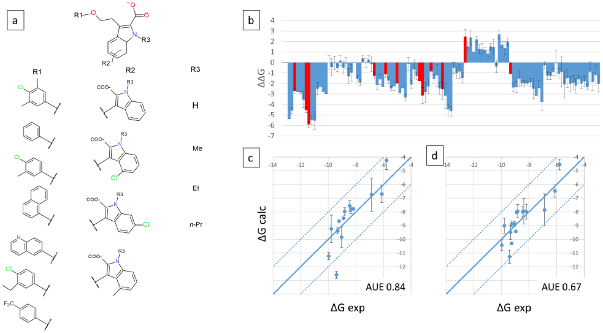
Three site MSLD system MCL1–6. Panel a shows the core ligand with three sites of substitutions or modifications, and the corresponding substituents or modifications. Panel b displays the calculated ΔΔG values for 109 out of 112 combinatorial ligands, with red bars indicating ligands for which experimental data is available. Panel c displays the calculated vs. experimental absolute binding free energies. Panel d displays binding free energies calculated using the additive approximation. Calculated relative free energies were converted to absolute by adding a constant offset value that minimizes errors associated with the choice of a single reference ligand as described in Methods. AUE are indicated on bottom right. Units are kcal/mol.

A second MCL1 system, MCL1–7 with two sites and 8×8 substituents was constructed as shown in Figure 11a. Site 1 substituents mostly differ by R-group substituents on the phenyl ring, except for sub4, which incorporates a napthyl group, whereas site2 substituents represent more diverse chemistry. 58/64 ligands were sampled during the production runs, predictions for which are displayed in Figure 11b. The ΔΔG values are calculated relative to a reference compound that models substituent 2, 1 on sites 1, 2 respectively (same compound as the one used in MCL1–6 system). The predictions show a large number of designs that bind significantly more strongly than the reference compound. 21 ligands have experimental data, indicated by red bars in Figure 11b. The non-additive and additive estimates of ΔG were calculated and are plotted in Figures 11c and 11d, respectively. The experimental data span 3.85 kcal/mol over which the AUE is 1.11 and 0.9 kcal/mol, respectively (Table 3).

Figure 11.

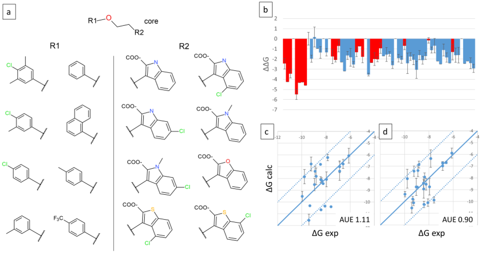
Three site MSLD system MCL1–7. Panel a shows the core ligand with two sites of substitutions, and the corresponding substituents. Panel b displays the calculated ΔΔG values for 58 out of 64 combinatorial ligands, with red bars indicating ligands for which experimental data is available. Panel c displays the calculated vs. experimental absolute binding free energies. Panel d displays binding free energies calculated using the additive approximation. Calculated relative free energies were converted to absolute by adding a constant offset value that minimizes errors associated with the choice of a single reference ligand as described in Methods. AUE are indicated on bottom right. Units are kcal/mol.

Finally, a third site was added to the HSP90–1 system to result in the three site HSP90–3 system with 6×5×3 substituents, shown in Figure S2 of Supporting Information. The methyl and ethyl substituents were added simply to evaluate the scalability; experimental data points for ligands with these substituents do not exist. In this system, only 68/90 ligands were sampled, predictions for which are displayed in Figure S2b. The ΔΔG values are calculated relative to a reference compound that models substituent 5, 1, 1 on sites 1, 2, 3 respectively (the ligand in the co-crystal structure 4YKR used in the simulations). The number of sampled ligands is lower than the other systems discussed above, which resulted in sampling a much larger fraction of the ligands modeled. This observation suggests that factors other than the number of substituents can impact sampling. Analysis of the number of transitions at each site revealed that the number of exchanges between site3-sub1 and sub2 or 3 are low. More than 1500 transitions are observed between sub2 and 3, in each 40ns trajectory segment, but the average number transitions involving sub1 are much lower at 97. While results for one and two site systems presented above suggest that statistics from such a number of transitions result in accurate predictions, for a three site system, the large number of combinations becomes prohibitively high. Experimental binding affinities are available for 9 ligands, out of which 5 were sampled, which are shown in Figure S2c. Figure S2d displays the additive estimates of free energies. Both estimates result in accurate predictions (Table 3), but the additive estimate is able to provide predictions for all 90 combinatorial ligands.

DISCUSSION

Given an accurate force field, explicit solvent based relative free energy methods can potentially offer accurate protein-ligand binding affinity predictions by virtue of an atomically detailed representation, and a rigorous statistical thermodynamic formulation. Both of these virtues are absent from several alternative methods for estimating binding affinity including docking-scoring methods, and implicit solvent based end-point methods including MM-GBSA and MM-PBSA.^{34, 35} Approximate methods are useful in prioritizing compounds from large sets, however the approximations employed have an unpredictable effect on the accuracy spanning different datasets and therefore render the methods less reliable. By contrast free energy methods are expected to be reliable based on the above cited considerations. In the recent past, several retrospective^{4–6, 36, 37} and prospective^{31, 33, 38} studies have shown free energy perturbation (FEP) to perform reliably for a large number of datasets and projects. However, relative FEP relies on ΔΔG estimates for pairs of ligands, which are obtained from calculations requiring tens of nanoseconds of sampling each, thus making the screening of large libraries of ligands computationally expensive. Multi-Site Lambda Dynamics (MSLD) offers a fundamentally different and efficient solution for the calculation of relative binding free energies.

Applicability domain.

Prior applications of MSLD have tested its applicability in estimating binding free energies of a chemical series that model both small modifications¹⁵ and substantially larger ones¹⁶. In this work, we chose an applicability domain motivated by the fact that MSLD simulations involve efficient transitions between substituents that are similar in volume or shape.¹² To illustrate this applicability domain, Figure 12a shows a representative screening scenario using ligands modeled in the MCL1 dataset supported by the presented validation, where different modifications to a core compound (circled in center) are modeled. MSLD simulations allow for all-to-all transitions (blue lines) and thus model a fully connected network. Figure 12b shows a contrasting example of a series of ligands beyond the scope of the ligand sets demonstrated in this study, in which the modifications involve larger changes (up to 16 heavy atoms) within the series. Blue arrows represent a minimal set of FEP calculations that allow the determination of affinities for this set. In principle, such large changes could still be modeled with MSLD, but longer simulations than used in this study may be needed to obtain accurate estimates. The applicability of the presented workflow to such cases will be the subject for a future study. Importantly, the hypothetical example shown in Figure 12a, and the real datasets modeled in this study Figures 1, 3–11 show that the method can still allow for the modeling of diverse substituents and modifications. For example, while R-group substituents were modeled in FAAH-2 (Figure 3) and CDK2–1 (Figure 7) systems, different heteroaromatic groups were included in MCL1–1 (Figure 1) and HSP90–2 (Figure 4) systems. The PTP1B-1 system (Figure 5) is an example of modeling differently sized rings. Different flexible alkyl chains were modeled in P38MK-4 (Figure 6) and TNKS2–2 (Figure 8) systems. These examples show the capability of the method to handle large differences in chemistry and topology, and therefore can be used to explore chemical space broadly.

Figure 12.

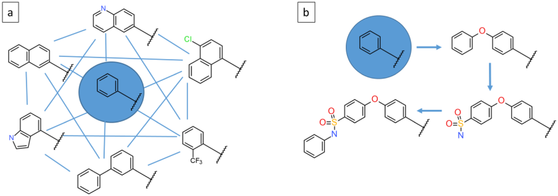
Example illustrating the domain of applicability of the presented MSLD workflow. Panel a shows a representative example with a core substituent, and a collection of substituents to explore chemical space in the neighborhood of the core. Blue lines indicate potential transitions during the MSLD simulations, which represents a fully connected network. Panel b shows an example of a series of ligands beyond the scope of the ligand sets demonstrated in this study. Arrows indicate a possible relative FEP calculation plan to cover this dataset, which represents a minimally connected FEP map.

Secondly, it is expected that a larger number of transitions and therefore better statistics would be related to a smaller number of substituents. Thus, one has to balance the desire to screen large libraries with the quality of statistics obtained. Figure S3 and accompanying text in the Supporting Information presents a detailed analysis of the number of transitions and its dependence on the number of substituents. The accurate predictions obtained with 8 or 9 substituent systems modeled in this study (eg. FAAH and CDK2) suggest that such a large number of substituents can be modeled accurately. We also note that 8 or 9 substituents have been identified in prior studies as an upper limit of the number of substituents that can be reliably modeled on a site.^{14, 15} A larger number of substituents can result in poorer statistics and lower confidence in the predictions. Finally, another requirement associated with the implemented method is that the sites should not have an overlap of atoms between them, and ideally be separated by a few bonds. Separation of a few bonds is required to avoid many inter-site shared valence parameters that may lead to instability during the simulations.

Additive Estimates.

An interesting result for systems modeling large combinatorial libraries (Table 3) is that additive free energy estimates were marginally more accurate than the cooperative estimates. This is somewhat surprising because additive estimates neglect the cooperative binding contributions from different sites. A possible reason for this could be better statistics for the additive estimates involving a larger number of substituent exchanges – for example, for the three site MCL1–6 system, the average number of single site transitions for the three sites are 864.8, 3431.3, and 2159.5 over 40ns. However, when transitions are calculated for the simultaneous occupancy of three sites, the corresponding average number is 48.9 (data not shown). It is anticipated that for systems that have strong inter-site coupling the additive approximation will become less accurate, even though it is not apparent in any of the systems tested here. This too may be the result of the design principles used in choosing how to delineate multi-site systems, whereby one or more bonds separated the branching of substituents likely reduced potential cooperative effects. Thus, it would be recommended to use the more rigorous cooperative estimates when available, and use additive estimates when the former is unavailable due to incomplete sampling. One prior MSLD application has shown scalability on larger combinatorial libraries¹⁵, but that study involved small substituents, used replica exchange to enhance sampling further, and more importantly, used about an order of magnitude more sampling than used here. In the interest of being of utility in fast paced lead optimization projects, the amount of sampling used in this study is much smaller, and yet shows good predictability.

While additive estimates do not explicitly incorporate cooperativity, MSLD by design is likely better suited than FEP to obtain additive estimates for combinatorial libraries. Since MSLD incorporates multiple sites in a single system, the effect of other sites on the exchange statistics of one site are represented in a “mean field” manner. If one were to do an analogous calculation with FEP, only a single site would be evaluated in each simulation, while fixing the other sites to an arbitrarily chosen substituent. The inclusion of multiple sites in a single system is a better approach in this scenario, and is a likely reason for obtaining accurate estimates in the five systems tested here (Table 3). Finally, it is noteworthy that the success seen here for the single-site additivity approximation combined with the large chemical spaces it opens to study, suggest that the application of such multi-site calculations would be of significant utility in establishing QSARs for a targeted scaffold.

Estimates obtained from reduced sampling.

Results presented above show the method’s efficiency in screening large compound sets. However, it is still of interest to test whether shorter simulation times could result in comparable accuracy, as that would enable screening of even larger libraries or number of systems given limited computing resources. To test the effect of sampling duration of MSLD production runs, the total sampling time was halved from 120ns to 60ns. Figure S4 and Table S1 in the Supporting Information show the AUE obtained for the seven subsets, and the five large combinatorial libraries, respectively. Results show only an insignificant drop in accuracy with reduced production sampling for the seven subsets. For large combinatorial libraries, reduced sampling results in lesser number of ligands being sampled, but the additive free energy estimates (Table S1) are nearly as accurate as those obtained with 120ns of sampling (Table 3). Thus, it may be possible to obtained accurate estimates with reduced sampling.

Another approach to gain efficiency was explored by obtaining free energy estimates from fixed biases provided by Phase 1, 2, and 3 of the bias optimization stages. The fixed bias estimates that are obtained from the bias optimization protocol estimate the end-state free energy, and together with the additive approximation can predict the binding free energies. Figure S4 and S5 in Supporting Information present the AUE obtained for the seven protein sets, and the five large combinatorial libraries, respectively. These results show that binding free energies obtained from fixed bias estimates have significantly reduced accuracy compared to those obtained from production simulations, and therefore the production stage is highly recommended for improved accuracy. Finally, the necessity of a three-phase bias optimization was examined by performing 120ns of cumulative production sampling, but initiated from Phase 1 and Phase 2 of the bias optimization stages. The analysis of the prediction metrics are detailed in the Supporting Information, with Tables S2–S4 listing the accuracy obtained with different levels of bias optimization. Results show that while for many sets, lesser bias optimization does not affect accuracy, for a few cases it leads to lack of sampling for a portion of the ligands (P38MK-7 and P38MK-8 systems). Given an additional computational cost per phase of only 10ns, it is recommended that the three-phase protocol be used for reliable performance.

Structural insights obtained from MSLD simulations.

In addition to binding free energy predictions, MSLD simulation trajectories can provide structural insights into the binding of different ligands modeled. Such information could be useful in generating additional design ideas that may result in improved affinity. For example, the Site2-sub4 group in P38MK-7 system is present among the six topmost favorable compounds, and it may be of utility to understand the interactions leading to the favorable affinity of ligands that include this substituent. Production simulation trajectories of the P38MK-7 system were analyzed visually to identify frames that coincide with the lambda value of Site2-sub4 being close to unity. This analysis revealed a water mediated interaction between the cyclohexanol alcohol group in Site2-sub4 and the carboxylate group of ASP109 in the protein. Figure 13a shows a representative snapshot displaying this water mediated interaction, where one of the two water molecules forms a water mediated hydrogen bond between the ligand and the protein.

Figure 13.

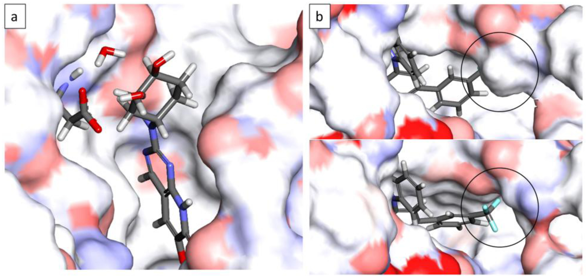
Representative snapshots chosen from MSLD simulation trajectories. Panel a shows the ligand with cyclohexanol group (Site2-sub4) from the P38MK-7 system forming a water-mediated hydrogen bond with the protein. The snapshot coincides with the lambda value of the substituent depicted being close to unity. Panel b shows the tri-fluoro phenyl group (Site1-sub8) from HSP90–2 system. Top sub-panel shows a snapshot corresponding to the lambda value of Site1-sub8 being close to zero, and the bottom sub-panel corresponds to the group interacting with the protein with a lambda value close to unity. The circled region shows a change in the protein conformation to accommodate the tri-fluoro group.

Another example of the structural and dynamical information gleaned from the simulations is from the HSP90–2 system, where the interaction of Site1-Sub8 group leads to widening of the protein pocket. The top panel in Figure 13b shows a representative frame corresponding to Site1-Sub8 being non-interactive, with its Lambda value close to zero, where the Tri-fluoro group clashes with the protein. The bottom panel shows a representative frame when its value is close to unity. The encircled region in the panels show a significant change in the shape of the protein pocket which is a consequence of the breaking an intra-protein hydrogen bond between THR94 sidechain and ASN91 backbone. This information can direct the use of relevant protein conformations in subsequent designs involving functionalization of this substituents to further enhance binding affinity.

Sampling of different conformational states of ligands.

Accuracy in free energy calculations requires the sampling of all thermodynamically relevant conformational states. This can be challenging when multiple stable conformational states exist and are separated by high free energy barriers. One prominent example of alternate conformational states are ortho and meta substituted phenyl rings frequently found in drug-like molecules. Typically, phenyl rings interact closely with the protein pocket which often prevents a rotation of the ring in the bound state, which leads to the sampling of only one of two conformational states during the free energy calculation, potentially leading to inaccurate results. Thus, as a general practice, initial conformations used in free energy calculations should be selected so as to favor the thermodynamically most favorable state as best as possible, doing which would at least ensure the more stable conformational state being sampled during the calculations. To this end, we used the automated Generated Analog Conformations²¹ method implemented in Discovery Studio (and Pipeline Pilot) that detects the different rotameric states automatically and identifies the most favorable using an MM-GBSA score. Thus, the initial conformations used in the free energy calculations here or in FEP are likely the thermodynamically favorable ones. However, limitations in scoring due to the implicit solvent approximation, or the occurrence of isoenergetic conformations may still limit accuracy. In such cases, MSLD by design offers a better and generalizable solution to sampling the different conformations during the simulations than pairwise FEP for two reasons. First, since multiple ligands are incorporated by means of the multi-topology ligand, the common core region is smaller than it would be in pairwise FEP, thus allowing for more flexibility for each substituent to explore different conformations. Second, in MSLD for long periods of sampling time during the course of the entire simulation individual substituents have lambda values close to zero when conformational transitions would be easy to achieve. By contrast, in FEP non-zero lambda values only exist in the end state windows, thus not allowing for such transitions during the remaining lambda windows. Figure 14 shows two examples of alternate conformational states being sampled during the protein-ligand complex MSLD simulations. Figure 14a shows FAAH-4 system where only the core atoms, and those belonging to substituent 1 are shown. Two phenyl ring orientations sampled during different times in the first simulation’s trajectory are shown, which position the Chlorine atom at the two locations. Figure 14b shows another example, that of the HSP90–2 system, where only the core atoms, and those of Site1-Subtituent 4 are shown. The two snapshots of the ligand show the two orientations of the phenyl ring that position the alcohol group differently. We note that not all systems with phenyl ring analogs modeled in this study allow the free rotation like the above two examples. For some systems (e.g. MCL1–1) part of the phenyl ring is included in the common core, which prevents substituents from independently accessing the two rotameric states. The extent of the common core is dependent on the extent of differences modeled and on the partial charge model used. In this study, bond charge increments²⁵ are used to assign partial charges, which typically result in minimizing the differences to a few atoms more than the chemical modifications themselves.

Figure 14.

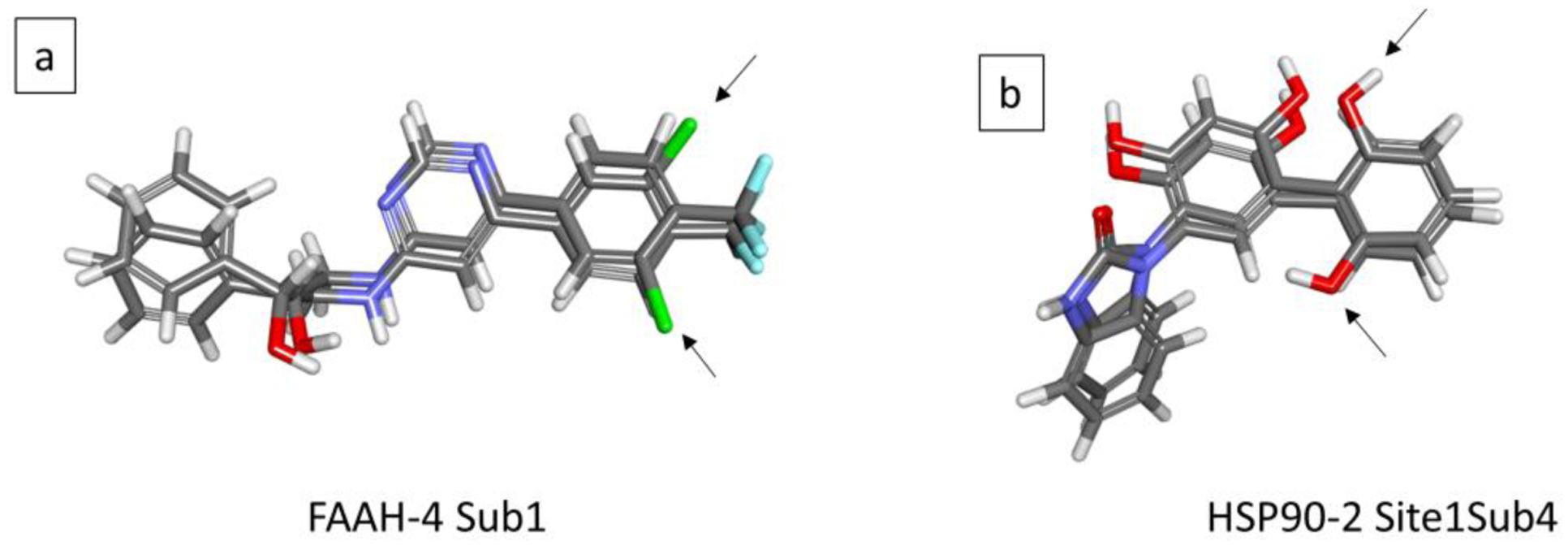
Two examples of alternate conformational states being sampled during the protein-ligand complex MSLD simulations. Panel a shows FAAH-4 system where only the core atoms, and those belonging to substituent 1 are shown. Two phenyl ring orientations sampled during different times in the first simulation’s trajectory are shown, which position the Chlorine atom at the two locations. Panel b shows another example, that of the HSP90–2 system, where only the core atoms, and those of Site1-Subtituent 4 are shown. The two snapshots of the ligand show the two orientations of the phenyl ring that position the alcohol group differently.

Computing Efficiency.

Several features of MSLD make the method more efficient relative to conventional FEP. Firstly, the dynamic treatment of lambda in combination with optimized biasing potentials enables the full thermodynamic transition between any pair of states to be modeled in a single simulation, where sampling is driven by the intrinsic chemical and conformational free energy landscape. In most FEP applications reported to date, a pre-determined lambda schedule is adopted which is independent of the free energy landscape and thus not necessarily the most efficient. Secondly, multiple ligands are modeled in a single simulation. In this study 19 single-site systems were tested which modeled 5–9 ligands each (Table 2). A cumulative sampling time of 150ns yielded predictive estimates from these systems. FEP applications that include cycle-closure edges typically use 1.5 * N relative FEP calculations to obtain absolute free energy estimates of N ligands.⁴ Assuming 60ns of sampling per relative FEP calculation, it amounts to 450 – 810 ns of sampling for 5 – 9 ligands. For single site MSLD systems used here, predictive estimates could be obtained with 3 to 5.4 fold less sampling than typical FEP applications. The two-site systems used in this study modeled 16 to 64 ligands, for which predictive estimates could be obtained with 150ns of cumulative sampling. For these systems, MSLD required 9.6 – 38.4 fold less sampling than FEP would have required, based on the above considerations. And finally, for three site systems, considering the 5×5×5 P38MK-7 as an example, predictive free energies were obtained with 75-fold less sampling. The error bars in the free energy plots shown in Figures 2, 9–11 indicate an acceptable degree of precision that would enable the use of the predictions in prioritizing compounds.

The throughput that can be obtained with the MSLD workflow is also dependent on the speed of the MD engine. As an example, the P38MK protein solvated in an orthorhombic shaped water box has 31,282 atoms. On this system, MSLD sampling of 32 ns can be obtained per day with the current implementation run on one NVIDIA GTX 1080 Ti card along with 4 CPUs. Thus, a typical calculation reported in this study would require 5 GPU days’ worth of resources, with minor additional resources for the free ligand system. The bias optimization stage with default parameters required 30ns or about 1 day on a single GPU. The production calculations running six trajectories on one GPU each require about 15 hours to finish 20ns. Thus, in less than 2 days of wall clock time, a large combinatorial library could be screened with small scale computing resources. Moreover, if three trajectories instead of six are chosen to run production calculations, it would reduce the computing resources requirements by 40%.

Best practices.

Based on the lessons we learned from the datasets and calculations described in this study, briefly summarized here are the factors to consider when applying the MSLD workflow to new systems. First, we note that the method implemented in its present form is most efficient for screening ligand substituents that span a similar volume or shape in the binding pocket. As shown above, this domain allows for screening chemically and topologically diverse groups. Second, to ensure sufficient sampling, our experience suggests that the number of substituents should not exceed nine at each site of modification. If a larger number of modifications is desired to be screened at a single site, the dataset can be split into multiple groups, with one common ligand serving as a reference within each group, as was done in the FAAH and CDK2 datasets, for example. We also note that such dataset splits would be straightforward to automate, though it was not done in this study. Third, when setting up multi-site systems, care must be taken to ensure that the site centers be separated by at least four bonds to prevent overlap between groups from two sites. Fourth, using a cumulative 120 ns of production sampling used in the workflow about 100 combinatorial ligands can be screened. However within the same frame of sampling, a larger number of ligands can be screened if estimates employing the additivity approximation are utilized. Our experience from these calculations suggest that this will likely be a good approximation in many cases. Finally, given the fact that accuracy was maintained with a reduced cumulative production sampling time of 60 ns, the workflow can be used with reduced sampling to improve throughput, especially screening relatively small libraries or when the additive approximation is used in multi-site systems.

CONCLUSIONS

This study presented an automated workflow that provides a framework to setup and execute the Multi-Site Lambda Dynamics (MSLD) free energy method to calculate relative binding affinities of combinatorial libraries of ligands. Given the specification of a core ligand with 1–3 well separated sites and a list of modifications, the workflow sets up simulation systems and executes the calculations. An automated protocol to iteratively optimize biasing potentials enabling enhanced sampling production simulations on a flattened free energy landscape is retrospectively validated on 31 MSLD systems spanning a wide range of chemical series and proteins. With a cumulative sampling time of 150ns, estimated binding free energies accurately predict experimental trends for datasets that include structurally diverse substituents. The presented method thus allows for accurate estimation of binding free energies of large combinatorial libraries with small scale GPU computing resources.

REFERENCES

- 1.Paul SM; Mytelka DS; Dunwiddie CT; Persinger CC; Munos BH; Lindborg SR; Schacht AL, How to Improve R&D Productivity: The Pharmaceutical Industry’s Grand Challenge. Nat Rev Drug Discov 2010, 9, 203–214. [DOI] [PubMed] [Google Scholar]
- 2.Muratov EN; Bajorath J; Sheridan RP; Tetko IV; Filimonov D; Poroikov V; Oprea TI; Baskin II; Varnek A; Roitberg A; Isayev O; Curtalolo S; Fourches D; Cohen Y; Aspuru-Guzik A; Winkler DA; Agrafiotis D; Cherkasov A; Tropsha A, QSAR without borders. Chem Soc Rev 2020. [DOI] [PMC free article] [PubMed] [Google Scholar]
- 3.Cournia Z; Allen B; Sherman W, Relative Binding Free Energy Calculations in Drug Discovery: Recent Advances and Practical Considerations. J Chem Inf Model 2017, 57, 2911–2937. [DOI] [PubMed] [Google Scholar]
- 4.Wang L; Wu Y; Deng Y; Kim B; Pierce L; Krilov G; Lupyan D; Robinson S; Dahlgren MK; Greenwood J; Romero DL; Masse C; Knight JL; Steinbrecher T; Beuming T; Damm W; Harder E; Sherman W; Brewer M; Wester R; Murcko M; Frye L; Farid R; Lin T; Mobley DL; Jorgensen WL; Berne BJ; Friesner RA; Abel R, Accurate and Reliable Prediction of Relative Ligand Binding Potency in Prospective Drug Discovery by way of a Modern Free-energy Calculation Protocol and Force Field. J Am Chem Soc 2015, 137, 2695–703. [DOI] [PubMed] [Google Scholar]
- 5.Song LF; Lee TS; Zhu C; York DM; Merz KM Jr., Using AMBER18 for Relative Free Energy Calculations. J Chem Inf Model 2019, 59, 3128–3135. [DOI] [PMC free article] [PubMed] [Google Scholar]
- 6.Bhati AP; Wan S; Wright DW; Coveney PV, Rapid, Accurate, Precise, and Reliable Relative Free Energy Prediction Using Ensemble Based Thermodynamic Integration. J Chem Theory Comput 2017, 13, 210–222. [DOI] [PubMed] [Google Scholar]
- 7.Kong X; Brooks CL III, Lambda-dynamics: A new approach to free energy calculations. J. Chem. Phys 1996, 105, 2414–2423. [Google Scholar]
- 8.Guo Z; Brooks CL III, Rapid Screening of Binding Affinities: Application of the λ-Dynamics Method to a Trypsin-Inhibitor System. J. Am. Chem. Soc 1998, 120, 1920–1921. [Google Scholar]
- 9.Banbaa S; Brooks CL III, Free energy screening of small ligands binding to an artificial protein cavity. J. Chem. Phys 2000, 113, 3423–3433. [Google Scholar]
- 10.Knight JL; Brooks CL III, Multi-Site lambda-dynamics for simulated Structure-Activity Relationship studies. J Chem Theory Comput 2011, 7, 2728–2739. [DOI] [PMC free article] [PubMed] [Google Scholar]
- 11.Knight JL; Brooks CL III, Applying efficient implicit nongeometric constraints in alchemical free energy simulations. J Comput Chem 2011, 32, 3423–32. [DOI] [PMC free article] [PubMed] [Google Scholar]
- 12.Armacost KA; Goh GB; Brooks CL III, Biasing Potential Replica Exchange Multisite lambda-Dynamics for Efficient Free Energy Calculations. J Chem Theory Comput 2015, 11, 1267–77. [DOI] [PMC free article] [PubMed] [Google Scholar]
- 13.Hayes RL; Armacost KA; Vilseck JZ; Brooks CL III, Adaptive Landscape Flattening Accelerates Sampling of Alchemical Space in Multisite lambda Dynamics. J Phys Chem B 2017, 121, 3626–3635. [DOI] [PMC free article] [PubMed] [Google Scholar]
- 14.Hayes RL; Vilseck JZ; Brooks CL III, Approaching protein design with multisite lambda dynamics: Accurate and scalable mutational folding free energies in T4 lysozyme. Protein Sci 2018, 27, 1910–1922. [DOI] [PMC free article] [PubMed] [Google Scholar]
- 15.Vilseck JZ; Armacost KA; Hayes RL; Goh GB; Brooks CL III, Predicting Binding Free Energies in a Large Combinatorial Chemical Space Using Multisite lambda Dynamics. J Phys Chem Lett 2018, 9, 3328–3332. [DOI] [PMC free article] [PubMed] [Google Scholar]
- 16.Vilseck JZ; Sohail N; Hayes RL; Brooks CL III, Overcoming Challenging Substituent Perturbations with Multisite lambda-Dynamics: A Case Study Targeting beta-Secretase 1. J Phys Chem Lett 2019, 4875–4880. [DOI] [PMC free article] [PubMed] [Google Scholar]
- 17.“BIOVIA Discovery Studio Modeling Environment, R. B., Dassault Systemes: San Diego, 2020. ”. [Google Scholar]
- 18.Berman HM; Westbrook J; Feng Z; Gilliland G; Bhat TN; Weissig H; Shindyalov IN; Bourne PE, The Protein Data Bank. Nucleic Acids Research 2000, 28, 235–242. [DOI] [PMC free article] [PubMed] [Google Scholar]
- 19.Spassov VZ; Yan L, A fast and accurate computational approach to protein ionization. Protein Sci 2008, 17, 1955–1970. [DOI] [PMC free article] [PubMed] [Google Scholar]
- 20.Best RB; Zhu X; Shim J; Lopes PE; Mittal J; Feig M; Mackerell AD Jr., Optimization of the additive CHARMM all-atom protein force field targeting improved sampling of the backbone phi, psi and side-chain chi(1) and chi(2) dihedral angles. J Chem Theory Comput 2012, 8, 3257–3273. [DOI] [PMC free article] [PubMed] [Google Scholar]
- 21.Raman EP, Template-Based Method for Conformation Generation and Scoring for Congeneric Series of Ligands. J Chem Inf Model 2019, 59, 2690–2701. [DOI] [PubMed] [Google Scholar]
- 22.Hassan M; Brown RD; Varma-O’brien S; Rogers D, Cheminformatics analysis and learning in a data pipelining environment. Mol Divers 2006, 10, 283–299. [DOI] [PubMed] [Google Scholar]
- 23.Lee MS; Feig M; Salsbury FR; Brooks CL III, New analytic approximation to the standard molecular volume definition and its application to generalized born calculations. Journal of Computational Chemistry 2003, 24, 1348–1356. [DOI] [PubMed] [Google Scholar]
- 24.Vanommeslaeghe K; Hatcher E; Acharya C; Kundu S; Zhong S; Shim J; Darian E; Guvench O; Lopes PEM; Vorobyov I; MacKerell AD Jr., CHARMM General Force Field: A Force Field for Drug-Like Molecules Compatible with the CHARMM All-Atom Additive Biological Force Fields. Journal of Computational Chemistry 2009, 31, 671–690. [DOI] [PMC free article] [PubMed] [Google Scholar]
- 25.Yesselman JD; Price DJ; Knight JL; Brooks CLI, MATCH: An Atom-typing Toolset for Molecular Mechanics Force Fields. J Comput Chem 2012, 33, 189–202. [DOI] [PMC free article] [PubMed] [Google Scholar]
- 26.Darden T; York D; Pedersen L, Particle mesh Ewald: an N•log(N) method for Ewald sums in large systems. J. Chem. Phys 1993, 98, 10089–10092. [Google Scholar]
- 27.Huang Y; Chen W; Wallace JA; Shen J, All-Atom Continuous Constant pH Molecular Dynamics With Particle Mesh Ewald and Titratable Water. J Chem Theory Comput 2016, 12, 5411–5421. [DOI] [PMC free article] [PubMed] [Google Scholar]
- 28.Brooks BR; Brooks III CL; MacKerell AD Jr.; Nilsson L; Petrella RJ; Roux B; Won Y; Archontis G; Bartels C; Boresch S; Caflisch A; Caves L; Cui Q; Dinner AR; Feig M; Fischer S; Gao J; Hodoscek M; Im W; Kuczera K; Lazaridis T; Ma J; Ovchinnikov V; Paci E; Pastor RW; Post CB; Pu JZ; Schaefer M; Tidor B; Venable RM; Woodcock HL; Wu X; Yang W; York DM; Karplus M, CHARMM: The biomolecular simulation program. J. Comput. Chem 2009, 30, 1545–1614. [DOI] [PMC free article] [PubMed] [Google Scholar]
- 29.Hynninen AP; Crowley MF, New faster CHARMM molecular dynamics engine. J Comput Chem 2014, 35, 406–13. [DOI] [PMC free article] [PubMed] [Google Scholar]
- 30.Rocklin GJ; Mobley DL; Dill KA; Hunenberger PH, Calculating the binding free energies of charged species based on explicit-solvent simulations employing lattice-sum methods: an accurate correction scheme for electrostatic finite-size effects. J Chem Phys 2013, 139, 184103. [DOI] [PMC free article] [PubMed] [Google Scholar]
- 31.Saha A; Shih AY; Mirzadegan T; Seierstad M, Predicting the Binding of Fatty Acid Amide Hydrolase Inhibitors by Free Energy Perturbation. J Chem Theory Comput 2018, 14, 5815–5822. [DOI] [PubMed] [Google Scholar]
- 32.Gathiaka S; Liu S; Chiu M; Yang H; Stuckey JA; Kang YN; Delproposto J; Kubish G; Dunbar JB Jr.; Carlson HA; Burley SK; Walters WP; Amaro RE; Feher VA; Gilson MK, D3R Grand Challenge 2015: Evaluation of Protein-ligand Pose and Affinity Predictions. J Comput Aided Mol Des 2016, 30, 651–668. [DOI] [PMC free article] [PubMed] [Google Scholar]
- 33.Christina S; Hannah B; Andreas B; Dietrich B; Hans-Peter B; Lars B; Daniel C; Eugene C; Paul C; Dieter D; Merveille E; Bruce F; Thomas F; Ulrich G; Jakub G; Theresa J; Catherine JL; Srinivasa K; Markus K; Lisa K; Tim K; Mireille K; Matthias L; Birgitta L; Liwei L; Igor M; Djordje M; Constantin N; Friedrich R; Kai S; Robert S; Thomas S; Eva-Maria T; Andrea UL; Ariele VF; Ansgar W; Daniel K, Large-Scale Assessment of Binding Free Energy Calculations in Active Drug Discovery Projects. 2020. [DOI] [PubMed]
- 34.Kollman PA; Massova I; Reyes C; Kuhn B; Huo S; Chong L; Lee M; Lee T; Duan Y; Wang W; Donini O; Cieplak P; Srinivasan J; Case DA; Cheatham TE 3rd, Calculating structures and free energies of complex molecules: combining molecular mechanics and continuum models. Acc Chem Res 2000, 33, 889–97. [DOI] [PubMed] [Google Scholar]
- 35.Brown SP; Muchmore SW, Large-scale application of high-throughput molecular mechanics with Poisson-Boltzmann surface area for routine physics-based scoring of protein-ligand complexes. J Med Chem 2009, 52, 3159–3165. [DOI] [PubMed] [Google Scholar]
- 36.Perez-Benito L; Casajuana-Martin N; Jimenez-Roses M; van Vlijmen H; Tresadern G, Predicting Activity Cliffs with Free-Energy Perturbation. J Chem Theory Comput 2019, 15, 1884–1895. [DOI] [PubMed] [Google Scholar]
- 37.He X; Liu S; Lee TS; Ji B; Man VH; York DM; Wang J, Fast, Accurate, and Reliable Protocols for Routine Calculations of Protein-Ligand Binding Affinities in Drug Design Projects Using AMBER GPU-TI with ff14SB/GAFF. ACS Omega 2020, 5, 4611–4619. [DOI] [PMC free article] [PubMed] [Google Scholar]
- 38.Kuhn B; Tichy M; Wang L; Robinson S; Martin RE; Kuglstatter A; Benz J; Giroud M; Schirmeister T; Abel R; Diederich F; Hert J, Prospective Evaluation of Free Energy Calculations for the Prioritization of Cathepsin L Inhibitors. J Med Chem 2017, 60, 2485–2497. [DOI] [PubMed] [Google Scholar]
Associated Data
This section collects any data citations, data availability statements, or supplementary materials included in this article.