COVID-19 intervention models: An initial aggressive treatment strategy for controlling the infection

Abstract

The novel coronavirus (COVID-19) outbreak emerged in December 2019. The disease has caused loss of many lives and has become an unprecedented threat to public health worldwide. We develop simple COVID-19 epidemic models to study treatment strategies to control the pandemic. The results show that eradication of the disease is possible if the efficacy of treatment is perfect. We also investigate the existence of a dual-rate effect. Conditions under which the effect occurs are derived. When the effect is present, a tactic to control the infection might be to initially treat infected individuals aggressively at a relatively high rate to drive the prevalence to a lower region that can be maintained in the long run at relatively moderate rate and cost.

1. Introduction

Coronavirus is a pathogen that targets the human respiratory system. It is mostly refereed to as COVID-19. The World Health Organization (WHO) officially named it the severe acute respiratory syndrome coronavirus 2 (SARS-CoV-2). The WHO declared the outbreak of SARS-CoV-2 a Public Health Emergency of International Concern on 30 January 2020 (Zheng et al., 2020). Compared with the SARS-CoV that caused an outbreak of SARS in 2003, SARS-CoV-2 has a stronger transmission capacity. It belongs to the same family of previous outbreaks of coronaviruses (CoVs), namely, severe acute respiratory syndrome (SARS)-CoV and the Middle East respiratory syndrome (MERS)-CoV. These are characterized as agents that are a great public health threat. Patients were admitted to hospitals with an initial diagnosis of pneumonia of an unknown etiology in late December 2019 Wuhan, Hubei Province, China. These patients were epidemiologically linked to a seafood and wet animal wholesale market in China, in the Hubei Province (Bogoch et al., 2020; Lu et al., 2020 ). This seafood and wet animal wholesale market sold live animals such as poultry, bats, marmots, and snakes.

The coronavirus has caused a lot of damage economically, health wise and otherwise. Service-oriented economies will be particularly negatively affected, and have more jobs at risk. Countries that are more reliant on tourism (more than 15% of GDP) will be more affected by this crisis. This current crisis is generating spillover effects throughout supply chains. Therefore, countries highly dependent on foreign trade are more negatively affected. Research study suggests that on average, each additional month of crisis costs 2.5–3% (Fernandes, 2020) of global GDP. Since the beginning of the virus, we have about seven million cases and approximately four hundred thousands deaths (Worldometer, 2020) with the United States having the highest cases as of June 2, 2020. Almost 50% of the cases have recovered worldwide. To contain the spread of the coronavirus, the WHO suggested that people should wash their hands with soap for more than two minutes, maintain social distancing, wear masks in public spaces, effective mass testing, lockdowns towns where the infection rates are higher. These lockdowns were meant to prepare governments to buy adequate health equipments in order to minimize casualties in terms of death. Many countries embarked on effective testing, had total lockdowns for almost two months in order to minimize the spread of the coronavirus. Some managed to fumigate public places, effectively tested large percentages of their populations. Countries like South Korea, Taiwan, New Zealand managed to bring down a lot of their cases in a short space of time due to their effective mass testing strategies. However, despite all these efforts, the coronaviruses cases spike up once the economy is re-opened. The best solution in containing the virus is getting some treatment drugs.

Several studies have been done on medications for treating COVID-19 patients. Cai et al., 2020 examined the effects of favipiravir (FPV) versus lopinavir (LPV)/ritonavir (RTV) for the treatment of COVID-19. They discovered that favipiravir showed better therapeutic responses on COVID-19 in terms of disease progression and viral clearance and hence one of the potential drugs for treatment. Many researchers (Felsenstein et al., 2020; Zhai et al., 2020) also worked on the remdesivir drug. Remdesivir has been recently a strong candidate for the treatment of COVID-19 and exhibits broad-spectrum antiviral activity against RNA viruses. Zhai et al. (2020) worked analyzing the different treatment drugs that have been tried in different clinical trials. Felsenstein et al. (2020) also analyzed different treatment drugs and their efficacy on reducing fatalities. They observed that the following anti-viral treatment drugs are potential treatment drugs for COVID-19. One of them is chloroquine which has antiviral activity against Influenza, Chikungunya virus, seasonal CoVs, and SARS. Another anti-viral treatment drug which is known as azithromycin is sometimes used for its immunomodulatory properties, especially in patients with chronic pulmonary disorders (Gensel et al., 2017; Haydar et al., 2019). Felsenstein et al. (2020) reported that convalescent plasma, i.e. plasma from individuals following COVID-19 resolution and rich in immunoglobulins directed against SARS-CoV2, is being entertained as possible treatment option. However, many clinical trials are being undertaken to determine the best treatment drug.

These medications once developed will be useful in mitigating the spread of the coronavirus. However, the question is, what should be the optimal way of administering the medications so that the virus is contained? In this paper, we try to answer this question by using the idea of dual-rate effect analysis. This effect has extensively studied in (Oduro, 2016; Oduro et al., 2018, 2019) and has shown to occur several models, including the re-infestation models in (Oduro, 2016; Oduro et al., 2018, 2019) and black pod disease model in (Oduro et al., 2020). In (Oduro et al., 2019), Oduro et al. stated that “the dual-rate effect has important implications for control efforts, as in the presence of this effect a strategy of adopting a highly aggressive short-term intervention at the beginning of a sustained control program may be more cost-effective in the long run than treatment at a fixed rate without a heightened initial effort”. We study compartmental COVID-19 models that incorporate treatment as a control measure with the ultimate goal of assessing optimal treatment strategies and deriving recommendations. These models were inspired by efforts to eradicate or contain the COVID-19 pandemic. The results reported here are purely mathematical and more widely applicable. They may be of particular relevance to the virus control efforts in lower middle-income countries (LMIC) where funds for the COVID-19 control programs are severely limited and often in competition for funds with one another as well as with other pressing health care needs and sectors such as education and infrastructure.

The rest of the paper is organized as follows, in Section 2, we formulate and analyze simple SEIR models. Dual-rate effect analysis are done in Sections 3. We then summarize the results in Section 4.

2. COVID-19 models with treatment

In this section we present two mathematical models, the first one with 100% efficacy of treatment and the second one with less than 100% efficacy of treatment.

2.1. Models formulation and their properties

2.1.1. First scenario: 100% efficacy of treatment

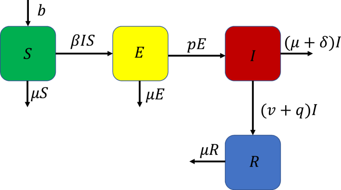
In this model, we assume that the population can be subdivided into four compartments. These are the susceptible (S) class, exposed (E) class, infected (I) class and lastly the recovered (R) class. The susceptible class recruits new population at the rate b. In all four classes, the natural death rate is given by μ and the mortality due to COVID-19 is given by δ. The transmission rate is given by β and the progression rate of exposed individuals to infected individuals is given by p. The infected individuals are treated with a recommended COVID-19 medication at rate v. These infected individuals can also be given other medical therapy at the rate q. The combination of the treatment and other medical therapy ensures that the infected individuals recover. The dynamics explained in this subsection are displayed in Fig. 1.

Fig. 1.

Dynamics of COVID-19 with 100% treatment.

The dynamics in Fig. 1 can be represented as a system of nonlinear ordinary differential equations given by

$$\begin{array}{cc}\frac{dS}{dt}& =b-\beta IS-\mu S\\ \frac{dE}{dt}& =\beta IS-(p+\mu )E\\ \frac{dI}{dt}& =pE-(q+v+\delta +\mu )I\\ \frac{dR}{dt}& =(q+v)I-\mu R.\end{array}$$ (1)

We summarize the existence of equilibrium in the following theorem.

Theorem 2.1

Consider the model 1.

• (i)The control reproduction number (${\mathcal{R}}_c$) is given by

$${\mathcal{R}}_c=\frac{\beta pb}{\mu (p+\mu )(q+v+\delta +\mu )}.$$

• (ii)When ${\mathcal{R}}_c\le 1$, then the disease-free equilibrium $DFE=\left(\frac{b}{\mu },0,0,0\right)$ is the only biologically feasible equilibrium.
• (iii)When ${\mathcal{R}}_c>1$, then in addition to the DFE, there exists a unique endemic equilibrium $EE=\left(S^{\ast },E^{\ast },I^{\ast },R^{\ast }\right)$ with

$$I^{\ast }=\frac{\beta pb-\mu (p+\mu )(q+v+\delta +\mu )}{\beta (p+\mu )(q+v+\delta +\mu )}=\frac{pb}{(p+\mu )(q+v+\delta +\mu )}-\frac{\mu }{\beta }=\frac{\mu }{\beta }\left({\mathcal{R}}_0-1\right).$$

2.1.2. Second scenario: less 100% efficacy of treatment

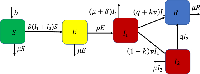
In this model, we assume that the population can be subdivided into five compartments. These are the susceptible (S) class, exposed (E) class, infected (I₁) class, infected (I₂) class after receiving ineffective treatment, and lastly the recovered (R) class. The recruitment rate is denoted by b, the natural mortality rate by μ and the mortality rate due to COVID-19 by δ. The transmission rate is given by β and the progression rate of exposed individuals to infected individuals is given by p. The infected individuals are treated at rate v. These infected individuals can also be given other medical therapy at the rate q. However, if the treatment is ineffective, then the individuals from I₁ move to I₂ at the rate (1 − k)v where k is the fraction of individuals who have been successfully treated with recommended COVID-19 medication. Thus those who have been successfully treated progress to the recovered class from the infected class I₁. The combination of the COVID-19 medication and other medical therapy ensures that the infected individuals recover. Fig. 2 shows the dynamics explained in this subsection.

Fig. 2.

Dynamics of COVID-19 with imperfect treatment.

The dynamics in Fig. 2 can be represented as a system of nonlinear ordinary differential equations of the form:

$$\begin{array}{cc}\frac{dS}{dt}& =b-\beta (I_1+I_2)S-\mu S\\ \frac{dE}{dt}& =\beta (I_1+I_2)S-(p+\mu )E\\ \frac{d{I}_1}{dt}& =pE-(q+v+\delta +\mu )I_1\\ \frac{d{I}_2}{dt}& =(1-k)v{I}_1-(q+\delta +\mu )I_2\\ \frac{dR}{dt}& =kv{I}_1+q(I_1+I_2)-\mu R.\end{array}$$ (2)

We summarize the existence of equilibrium in the following theorem.

Theorem 2.2

Consider the model 2.

• (i)The control reproduction number (${\mathcal{R}}_c$) is given by

$${\mathcal{R}}_{\mathbf{c}}=\frac{bp\beta (q+\delta +\mu +(1-k)v)}{\mu (q+\delta +\mu )(p+\mu )(q+v+\delta +\mu )}.$$

• (ii)When ${\mathcal{R}}_c\le 1$, then the disease-free equilibrium $DFE=\left(\frac{b}{\mu },0,0,0,0\right)$ is the only biologically feasible equilibrium.
• (iii)When ${\mathcal{R}}_c>1$, then in addition to the DFE, there exists a unique endemic equilibrium $EE=\left(S^{\ast },E^{\ast },I_1^{\ast },I_2^{\ast },R^{\ast }\right)$ with

$$\begin{array}{cc}{I}_1^{\ast }& =\frac{bp\beta (q+\delta +\mu +(1-k)v)-\mu (q+\delta +\mu )(p+\mu )(q+v+\delta +\mu )}{\beta (q+\delta +\mu +(1-k)v)(p+\mu )(q+v+\delta +\mu )}\\ I_1^{\ast }& =\frac{\mu (q+\delta +\mu )\left({\mathcal{R}}_0-1\right)}{\beta (q+\delta +\mu +(1-k)v)}.\end{array}$$

2.2. Model fitting

We use Pennsylvania (USA) state-level time series for cumulative active COVID-19 cases compiled by Worldometer (Worldometer, 2020), from March 15, 2020, through May 31, 2020 to estimate the model parameters. The sources of the data provided by Worldometer were checked for confirmation. The model fitting was performed using the standard nonlinear least squares approach using the fmincon Optimization Toolbox embedded in MATLAB. We provide the estimated parameters in Table 1. The recruitment rate was estimated from the population data for Pennsylvania, by US Census Bureau (US Census Bureau) and the natural death rate was adopted from the National Center for Health Statistics (National Center for Health Statistics).

Table 1.

Parameters and their meanings.

Parameter	Value	Unit
β (transmission rate)	4.511e − 07	day−1
b (recruitment rate)	9213	–
p (progression rate of exposed individuals to infected)	0.3571	day−1
v (COVID-19 treatment rate)	varies (0.4665)	–
q (other medication therapy rate)	0.420	day−1
δ (disease mortality rate)	0.0141	day−1
μ (natural mortality rate)	0.008638	–
S(0) (Initial value of the susceptible)	12797248	Individuals
E(0) (Initial value of the expose)	2729	Individuals
I(0) (Initial value of infected)	19	Individuals
R(0) (Initial value of recovered)	2	Individuals
${\mathcal{R}}_c=1.5006$ (For scenario 1)
${\mathcal{R}}_c=1.7873$ (For scenario 2)

2.3. Effect of COVID-19 treatment

Since the treatment rate, v, is our man control parameter, let us consider the effect of this parameter on the control reproduction number for both models.

Scenario 1: The partial derivative w.r.t v is

$$\begin{array}{cc}\frac{\partial {\mathcal{R}}_c}{\partial v}& =-\frac{\beta pb}{\mu (p+\mu ){(q+v+\delta +\mu )}^2}<0.\end{array}$$ (3)

Thus, the ${\mathcal{R}}_c$ is non-increasing with respect to v. Also

$$\underset{v\to \infty }{\lim }{\mathcal{R}}_c=0.$$

This suggests that eradication will be achieved with sufficiently high treatment rate, the control reproduction number decreases significantly as the treatment rate increases.

Scenario 2:

We have

$$\begin{array}{cc}\frac{\partial {\mathcal{R}}_c}{\partial v}& =-\frac{\beta pbk}{\mu (p+\mu ){(q+v+\delta +\mu )}^2}<0.\end{array}$$

and

$$\underset{v\to \infty }{\lim }{\mathcal{R}}_c=\frac{bp\beta (1-k)}{\mu (q+\delta +\mu )(p+\mu )}.$$ (4)

The ${\mathcal{R}}_c$ decreases with v but asymptotically approaches the right-hand side of 4. This suggests that with some parameter settings, high treatment rate may not be sufficient to eradicate the disease.

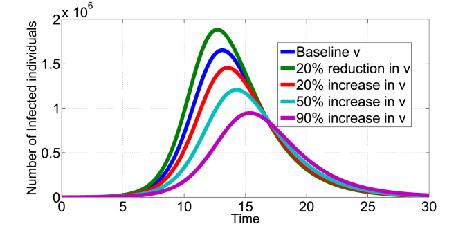
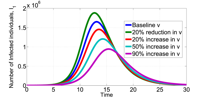
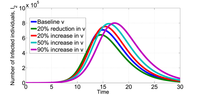
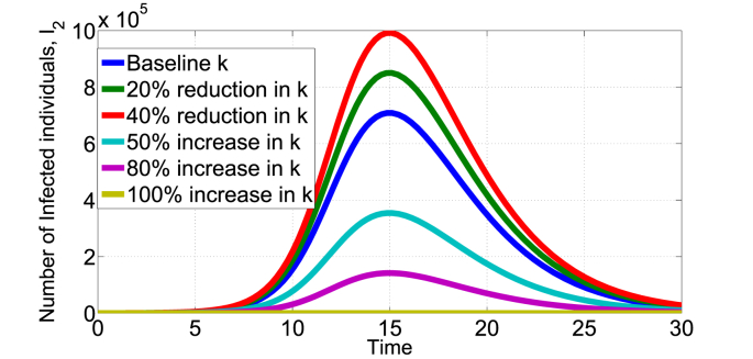
Fig. 3, Fig. 4, Fig. 5 show the effect of varying the treatment rate, v, on the infectious class in scenario 1 and 2 respectively. The values of parameters used are as given in Table 1 unless otherwise stated. First, increasing the treatment rate decreases the population of infected individuals as shown in Fig. 3, Fig. 4. We also note that decreasing the treatment rate increases the population of infected individuals. The treatment intervention delays the peak of the epidemic curve and thus reduces the number of infested individuals. Second, Fig. 5 shows the effect of treatment on the infected population that still remain infected after being treated (Scenario 2). Of course, the potency of the treatment will play a major factor, fixing k = 0.8 and increasing the treatment rate leads to increase in the I₂(t) infected population as shown in Fig. 5. Other medical therapies may be needed to contain individuals in the I₂(t) class if the COVID-19 treatment is not 100% effective. In Fig. 6, we show the effect of k (fraction of successfully COVID-19 treatment) on I₂(t). Increasing k, decreases the I₂(t) population. For example, increasing the baseline k = 0.5 by 50% reduces the population in I₂(t) from about 7 × 10⁵ to below 4 × 10⁵ individuals. Thus, the efficacy of the treatment has direct impact on this infected population.

Fig. 3.

Impact of COVID-19 treatment on I(t) in the scenario 1 model, baseline v = 0.4665.

Fig. 4.

Impact of COVID-19 treatment on I₁(t) in the scenario 2 model, baseline v = 0.4665.

Fig. 5.

Impact of COVID-19 treatment on I₂(t) in the scenario 2 model, baseline v = 0.4665.

Fig. 6.

Impact of k on I₂(t) in the scenario 2 model, baseline k = 0.5.

3. Treatment strategies

In this section, we investigate long-term cost effective strategies for controlling the COVID-19 infection. Assuming there is a recommended medication treatment, we show the existence of a dual-rate effect. When this effect is present, an initial aggressive treatment rate may plunge the prevalence to a level that can be controlled at a lower treatment rate and relatively moderate cost (Oduro, 2016; Oduro et al., 2018, 2019).

3.1. Preliminaries

In what follows, we provide some useful definitions with notations that are needed in subsequent section.

Let [T⁻, T⁺) be a given time interval of length T⁺ − T⁻ = ΔT. Then

$$Y_{T^{-},T^{+}}={\int }_{T^{-}}^{T^{+}}I(t)dt$$ (5)

is the overall cases of COVID-19 between T⁻ and T⁺. Following the approach in (Oduro, 2016; Oduro et al., 2018, 2019), we conceptualize the cost (C) as the total amount of treatment needed over the interval and it is defined as

$$C=v{\int }_{T^{-}}^{T^{+}}I(t)dt,$$ (6)

where v is the COVID-19 treatment rate. We established in Section 2.1 that when v is kept constant, the susceptible, exposed, infested, and recovered individuals approach an equilibrium, with I∗(v) denoting the number of infected individuals at equilibrium. If an endemic equilibrium can be reached, then the long-term cost of COVID-19 treatment can be conceptualized as follows:

$$C(v)=v{I}^{\ast }(v).$$ (7)

It is important to note that, the equilibrium value I∗(v) is a monotone decreasing function of v. However, under certain conditions the dependence of C on v is not monotone.

Definition 3.1

[Dual-rate effect]. Let I∗(v) be the number of infected individuals at equilibrium and C(v) be the cost of treatment at equilibrium. A dual-rate effect occurs if there exist two different treatment rates v₁ and v₂ such that

• i.C(v₁) = C(v₂),
• ii.I∗(v₁) < I∗(v₂).

We will use the following observation.

Proposition 3.1

If the cost function C(v) has a strict local maximum at some v ∈ (0, ∞), then the dual-rate effect occurs.

Proof. Let v_c be the critical point of C(v). Then there exist two distinct treatment rates v_l and v_h with v_l < v_c < v_h such that C(v_l) = C(v_h) < C(v_c). Since I∗ depends on the treatment rate and decreases monotonically with v, a low treatment rate 0 < v_l < v_crit will produce a relatively high I∗ and a high treatment rate v_c < v_h, will yield a relative low I∗. That is, I∗(v_l) > I∗(v_h). This implies that there is a cost C(v_l) = C(v_h) that corresponds to two different values of I∗(v).

3.2. Main results

We present results for dual-rate rate effect.

Theorem 3.1

Consider the model with perfect treatment efficacy and let $\beta >\frac{\mu (p+\mu )(q+\delta +\mu )}{pb}$. Then the dual-rate effect occurs whenever the endemic equilibrium exists.

Proof. Using the I∗(v) of the endemic equilibrium in Theorem 2.1 and the definition in equation (7), we have

$$C(v)=\frac{pbv}{(p+\mu )(q+v+\delta +\mu )}-\frac{\mu v}{\beta }.$$ (8)

It follows that

$$\frac{dC}{dv}=\frac{pb(q+\delta +\mu )}{(p+\mu ){(q+v+\delta +\mu )}^2}-\frac{\mu }{\beta }.$$ (9)

This yields a critical treatment rate $v^{\ast }=\sqrt{\frac{\beta pb(q+\delta +\mu )}{\mu (p+\mu )}}-(q+\delta +\mu )$, which is biologically meaningful if $\beta >\frac{\mu (p+\mu )(q+\delta +\mu )}{pb}$. Also,

$$\frac{d^{2}C}{d{v}^2}=-\frac{2pb(q+\delta +\mu )}{(p+\mu ){(q+v+\delta +\mu )}^2}<0.$$ (10)

By the second derivative test, the cost function C(v) has a local maximum value at v∗. The rest of the Proof follows directly from Proposition 3.1.

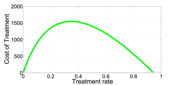
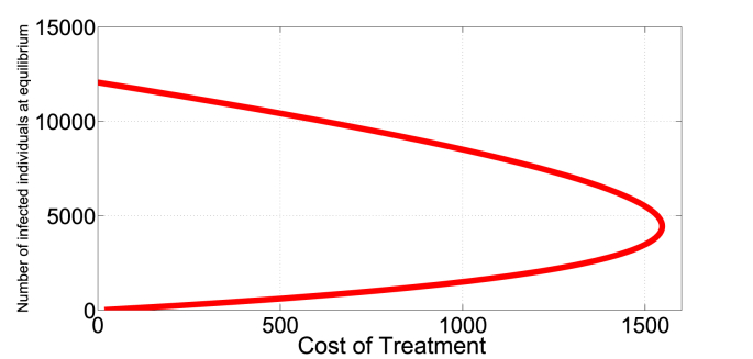
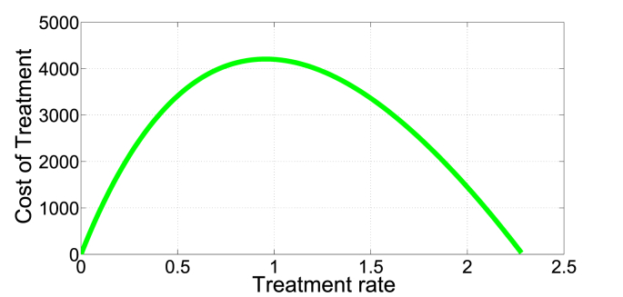
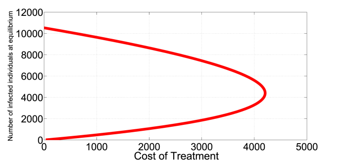
In Fig. 7, Fig. 8, we present an illustration of the presence of the dual-rate effect. For example, (with b = 9213, β = 1.386e − 06, μ = 0.008638, p = 0.2710, q = 0.4655, δ = 0.014067) a cost of 500 corresponds to two different treatment rates, approximately v₁ = 0.05 and v₂ = 0.8. Since the I∗ is a monotone decreasing function of v, I∗(0.05) = 612 individuals, a relatively low infection level than I∗(0.8) = 10419 individuals. Here, an optimal strategy is to initially treat at rate v = 0.8 to push the system into a region with low endemic level of infection that can be maintained in the long run at relatively low rate v = 0.05.

Theorem 3.2

Consider the model with imperfect treatment efficacy and let

$$\frac{\mu (q+\delta +\mu )(p+\mu )}{pb}<\beta <\frac{\mu (q+\delta +\mu )(p+\mu )}{{(1-k)}^{2}pb}.$$

Then the dual-rate effect occurs whenever the endemic equilibrium exists.

Proof. Similarly to the proof of Theorem 3.1, let

$$C(v)=\frac{bpv}{(p+\mu )(q+v+\delta +\mu )}-\frac{\mu (q+\delta +\mu )v}{\beta (q+\delta +\mu +(1-k)v)},$$ (11)

then

$$\begin{array}{cc}\frac{dC}{dv}& =\frac{bp(q+\delta +\mu )}{(p+\mu ){(q+v+\delta +\mu )}^2}-\frac{\mu {(q+\delta +\mu )}^2}{\beta {(q+\delta +\mu +(1-k)v)}^2}\\ \frac{d^{2}C}{d{v}^2}& =-\frac{2pb(q+\delta +\mu )}{(p+\mu ){(q+v+\delta +\mu )}^3}+\frac{2\mu {(q+\delta +\mu )}^2(1-k)}{\beta {(q+\delta +\mu +(1-k)v)}^3}.\end{array}$$ (12)

The critical treatment rate occurs at

$$v^{\ast }=\frac{(q+\delta +\mu )\left(\sqrt{\frac{\mu (q+\delta +\mu )(p+\mu )}{\beta pb}}-1\right)}{(1-k)-\sqrt{\frac{\mu (q+\delta +\mu )(p+\mu )}{\beta pb}}},$$

this holds if

$$\frac{\mu (q+\delta +\mu )(p+\mu )}{pb}<\beta <\frac{\mu (q+\delta +\mu )(p+\mu )}{{(1-k)}^{2}pb}.$$

For example, choosing $\beta =\frac{\mu (q+\delta +\mu )(p+\mu )}{(1-k)pb}$ gives

$$v^{\ast }=\frac{(q+\delta +\mu )\left(\sqrt{(1-k)}-1\right)}{(1-k)-\sqrt{(1-k)}}=\frac{(q+\delta +\mu )\left(\sqrt{(1-k)}-1\right)}{\sqrt{(1-k)}\left(\sqrt{(1-k)}-1\right)}=\frac{q+\delta +\mu }{\sqrt{1-k}}>0$$

and

$$\begin{array}{cc}\frac{d^{2}C}{d{v}^2}& =-\frac{2pb(q+\delta +\mu )}{p+u}\left[\frac{1}{{(q+\delta +\mu +v^{\ast })}^3}-\frac{{(1-k)}^2}{{(q+\delta +\mu +(1-k)v^{\ast })}^3}\right]\\ \frac{d^{2}C}{d{v}^2}& =-\frac{2pb(q+\delta +\mu )}{(p+u){(q+\delta +\mu +(1-k)v^{\ast })}^3}\left[{\left(\frac{q+\delta +\mu +(1-k)v^{\ast }}{q+\delta +\mu +v^{\ast }}\right)}^3-{(1-k)}^2\right]\\ & =-\frac{2pb(q+\delta +\mu ){(1-k)}^2}{(p+u){(q+\delta +\mu +(1-k)v^{\ast })}^3}\left[{\left(\frac{q+\delta +\mu +(1-k)v^{\ast }}{{(1-k)}^{2/3}(q+\delta +\mu +v^{\ast })}\right)}^3-1\right]\\ & =-\frac{2pb{(1-k)}^2}{(p+u){(q+\delta +\mu )}^2{(1+{(1-k)}^{1/2})}^3}\left[{\left(\frac{1+{(1-k)}^{1/2}}{\left({(1-k)}^{2/3}+{(1-k)}^{1/6}\right)}\right)}^3-1\right]\\ & =-\frac{2pb{(1-k)}^2}{(p+u){(q+\delta +\mu )}^2{(1+{(1-k)}^{1/2})}^3}\left(\frac{1}{\sqrt{1-k}}-1\right)<0\end{array}$$ (13)

for all 0 < k < 1.

Fig. 7.

Identical costs corresponding to two treatment rates.

Fig. 8.

Identical costs can produce two endemic equilibrium levels.

The cost function has a strict local maximum at v∗, the existence of the dual-rate effect follows from Proposition 3.1.

As illustrated in Fig. 9, Fig. 10, the dual rate occurs in this scenario where the efficacy of treatment is not perfect.

Fig. 9.

Identical costs carrying two different treatment rates.

Fig. 10.

Identical costs with two different endemic equilibrium levels.

4. Summary

In this paper, we designed and analyzed two mathematical models with treatment, one with 100% efficacy of the treatment and the other one with less than 100% efficacy of the treatment. We derived conditions for both disease-free and endemic equilibria to exist, and argued that the infection can be eradicated in the scenario with perfect efficacy of treatment if the treatment rate is sufficiently high. On the other hand, treatment may not be sufficient for eradication if the efficacy is not prefect. The prevalence can only be driven to arbitrarily low levels by sufficiently large treatment rate.

We also investigated the long-time cost effective strategies for controlling the COVID-19 infection. In particular, we showed the existence of the dual-rate effect in both models. When this effect is present, the optimal strategy might be an initially very aggressive treatment to plunge the prevalence to a level that can be controlled at a lower treatment rate and in the long run at relatively moderate cost. The high initial treatment rate may require a substantial initial investment (cost) which may payoffs in the long run. Without the initially very high treatment, the same average cost would only allow a much less significant reduction in long-term prevalence level.

Ethical approval

This article does not contain any studies with human participants performed by any of the authors.

Declaration of competing interest

All authors declared that no competing interests exist.

Handling editor: Dr. J Wu

References

- Bogoch I.I., Watts A., Thomas-Bachli A., Huber C., Kraemer M.U., Khan K. Pneumonia of unknown etiology in Wuhan, China: Potential for international spread via commercial air travel. Journal of Travel Medicine. 2020;27(2) doi: 10.1093/jtm/taaa008. [DOI] [PMC free article] [PubMed] [Google Scholar]
- Cai Q., Yang M., Liu D., Chen J., Shu D., Xia J., Shen C. Experimental treatment with favipiravir for COVID-19: An open-label control study. Engineering. 2020;6(10):1192–1198. doi: 10.1016/j.eng.2020.03.007. [DOI] [PMC free article] [PubMed] [Google Scholar]
- Felsenstein S., Herbert J.A., McNamara P.S., Hedrich C.M. COVID-19: Immunology and treatment options. Clinical Immunology. 2020:108448. doi: 10.1016/j.clim.2020.108448. [DOI] [PMC free article] [PubMed] [Google Scholar]
- Fernandes N.uno. March 22, 2020. Economic effects of coronavirus outbreak (COVID-19) on the world economy. [Google Scholar]
- Gensel J.C., Kopper T.J., Zhang B., Orr M.B., Bailey W.M. Predictive screening of M1 and M2 macrophages reveals the immunomodulatory effectiveness of post spinal cord injury azithromycin treatment. Scientific Reports. 2017;7(1):1–10. doi: 10.1038/srep40144. [DOI] [PMC free article] [PubMed] [Google Scholar]
- Haydar D., Cory T.J., Birket S.E., Murphy B.S., Pennypacker K.R., Sinai A.P., Feola D.J. Azithromycin polarizes macrophages to an M2 phenotype via inhibition of the STAT1 and NF-KB signaling pathways. The Journal of Immunology. 2019;203(4):1021–1030. doi: 10.4049/jimmunol.1801228. [DOI] [PMC free article] [PubMed] [Google Scholar]
- Lu H, Stratton CW, Tang YW. Outbreak of pneumonia of unknown etiology in Wuhan, China: The mystery and the miracle. Journal of Medical Virology. 2020 Apr;92(4):401–402. doi: 10.1002/jmv.25678. Epub 2020 Feb 12. PMID: 31950516; PMCID: PMC7166628. [DOI] [PMC free article] [PubMed] [Google Scholar]
- National Center for Health Statistics https://www.cdc.gov/nchs/fastats/deaths.htm
- Oduro B. 2016. http://rave.ohiolink.edu/etdc/view?acc-num=ohiou1458563770 Ph.D. dissertation.
- Oduro B., Apenteng O.O., Nkansah H. Assessing the effect of fungicide treatment on Cocoa black pod disease in Ghana: Insight from mathematical modeling. Statistics, Optimization & Information Computing. 2020;8(2):374–385. doi: 10.19139/soic-2310-5070-686. [DOI] [Google Scholar]
- Oduro B., Grijalva M.J., Just W. Models of disease vector control: When can aggressive initial intervention lower long-term cost? Bulletin of Mathematical Biology. 2018;80(4):788–824. doi: 10.1007/s11538-018-0401-y. [DOI] [PubMed] [Google Scholar]
- Oduro B., Grijalva M.J., Just W. A model of insect control with imperfect treatment. Journal of Biological Dynamics. 2019;13(NO. 1):518–537. doi: 10.1080/17513758.2019.1640293. [DOI] [PubMed] [Google Scholar]
- US Census Bureau https://www.census.gov/topics/population.html
- Worldometer 2020. https://www.worldometers.info/coronavirus/
- Zhai P., Ding Y., Wu X., Long J., Zhong Y., Li Y. The epidemiology, diagnosis and treatment of COVID-19. International Journal of Antimicrobial Agents. 2020:105955. doi: 10.1016/j.ijantimicag.2020.105955. [DOI] [PMC free article] [PubMed] [Google Scholar]
- Zheng Y., Ma Y., Zhang J., Xie X. COVID-19 and the cardiovascular system. Nature Reviews Cardiology. 2020;17:259–260. doi: 10.1038/s41569-020-0360-5. [DOI] [PMC free article] [PubMed] [Google Scholar]