Open-source computational framework for studying Drosophila behavioral phase

Summary

This protocol describes a standardized method for analyzing Drosophila behavioral rhythmicity under light dark cycles, temperature ramps, and free running conditions. The protocol constitutes a step-by-step guide from generation of appropriate Drosophila genetic crosses to behavioral experiments. We also provide an open-source computational framework using R for the analysis of the phase of behavior using circular statistics. An extended method for complete use is also provided.

For complete details on the use and execution of this protocol, please refer to Fernandez et al. (2020).

Graphical Abstract

Highlights

• •R framework for analysis of Drosophila behavioral phase and circular statistics analysis
• •Visualization of activity, phase of behavior, and rose plots

This protocol describes a standardized method for analyzing Drosophila behavioral rhythmicity under light dark cycles, temperature ramps, and free running conditions. The protocol constitutes a step-by-step guide from generation of appropriate Drosophila genetic crosses to behavioral experiments. We also provide an open-source computational framework using R for the analysis of the phase of behavior using circular statistics. An extended method for complete use is also provided.

Before you begin

Experimental design: plan genetic crosses

Timing: 1 h

• 1.
  Design the crossing scheme for the desired F1 offspring. Assume that for most crosses kept at 25°C, F1 will be ready to load into the activity monitors ~15 days after the crosses are set (11 days to have progeny + 3–4 days to let the adult flies age).

  • a.
    For example, to obtain F1 in which the s-LNv arbor is truncated as previously described (Fernandez et al., 2020), w;Pdf(BMRJ)-Gal4/CyO; females should be crossed to w;;UAS-Unc5-HA males (see Key resources table).
  • b.
    Ideally, crosses should have replicates set up on the same day, plan accordingly when collecting flies.

CRITICAL: Make sure that the combination of balancer chromosomes, if applicable, will lead to sufficient progeny and plan to select against balancers in the appropriate developmental stage (Chyb and Gompel, 2013).

Virgin female collection

Timing: 3–7 days

• 2.4 weeks prior to the desired experiment start date, begin to collect Drosophila virgin females. For the best collection results, we recommend clearing the fly bottles or vials in the early morning and collecting every 3–5 h throughout the day.
• 3.Repeat collection process until each cross has 8–12 virgin females per vial.

CRITICAL: Virgin females older than ~10 days will yield less progeny.

Fly rearing and crosses

Timing: 2–3 weeks

• 4.
  Day 0: ~20 days prior to the experiment start date (the exact time depends on genotype and environmental conditions, particularly temperature), set up the fly crosses. Collect 4–5 males of the desired genotypes and place them in vials containing fly media with their respective virgin females.

  • a.
    Each cross should be duplicated to ensure sufficient F1 for loading.
  • b.
    Make sure the males are healthy, young (3–7 days old) and do not have damaged wings.
• 5.Day 5: Flip all crosses into fresh vials once it is clear that abundant larvae are present in the media, this is critical to avoid parental and F1 flies from mixing. Save the flipped vials for more F1 progeny to be loaded in a second trial, if desired.

• 6.
  Day 5: Place the original vials in an incubator set for proper entertainment conditions. This ensures F1 will be in the correct environmental conditions upon eclosion.

  Note: if this is not possible due to incubator availability, flies may have to be kept in the environmental condition of the experiment for longer.

  • a.
    For standard entrainment conditions we recommend keeping flies at 25°C under a 12:12 Light Dark (LD) cycle for at least 3 days. Ideally, the LD cycle timing should match that of the behavioral experiment. If the light regime timing used for rearing differs significantly from that of the behavioral experiment, should be given more time under LD to re-entrain (Helfrich-Forster et al., 2001).
  • b.
    For experiments involving entrainment temperature ramps we recommend rearing flies at 25°C under constant darkness from the time the crosses are set until the progeny is loaded into activity monitors.

• 7.Day 11: Begin to collect F1 males as they eclose. Keep them in small groups (4–8 flies) until the time of the experiment.

Note: Virgin females can be used as well (mated females would lay eggs on the food, which could be overcome by shortening the duration of the experiments).

• 8.Day 16: Clear the adults from the second flip if a second behavioral run is desired from the same crosses. Repeat steps 6 and 7 with these vials.

CRITICAL:

• -Vials with crosses should not be overcrowded or F1 flies will be too small and may exhibit abnormal behavior.
• -F1 can only be collected up to 18 days from the day the cross was set up (conservatively) to ensure that there are no F2 offspring among the flies.

Activity monitor tube preparation

Timing: 2 h

• 9.
  Prepare tubes at least two days prior to running the experiment. If prepared earlier, make sure to refrigerate and keep covered. Begin by preparing a food solution.

  • a.
    Obtain sufficient numbers of Trikinetics 5 mm tubes for the experiment, and include extra tubes. Each Drosophila Activity Monitor (DAM) can hold 32 tubes and we recommend at least one full monitor per genotype. Ideally, tubes should be autoclaved before use. To prepare 310 tubes use a 500 mL Erlenmeyer flask. Add 5 g of Bacto agar and 10 g of sucrose. Then add 250 mL of deionized water.
  • b.
    Microwave (1,000 watts) for ~45 s. Carefully remove the flask and stir with a glass rod. Place the flask back into the microwave for 30 s, remove, and stir solution with a glass rod. Continue microwaving in 10-s increments and stirring until a clear solution is attained.
  • c.
    Split the solution into 2 × 1,000 mL beakers.
  • d.
    Place tubes into bundles of approximately 32 tubes using rubber bands. Carefully place the bundles into the beakers making sure that the tubes are perpendicular to the bottom of the beaker and the food solution is evenly distributed within all tubes.
  • e.
    Once all bundles are placed in the liquid, cover beakers with a piece of paper towel and secure with a rubber band. This will prevent contamination.
  • f.
    Place the beakers in a cold room or refrigerator at 4°C for 4–24 h.
• 10.
  Seal the tubes using paraffin wax.

  • a.
    Carefully remove tubes from the beaker. Discard any tubes that do not contain at least 1 cm of solid agar that lacks air bubbles.
  • b.
    Place the tubes in a container under a fume hood. Within the fume hood, gather a hot plate, a crucible, paraffin wax, and a second crate lined with paper towels. Turn the hotplate to 250°C–300°C. Place the crucible on top of the hot plate fill with paraffin wax to approximately 5 cm depth.
  • c.
    Allow the paraffin wax to melt until entirely liquid, then reduce heat of the hotplate to low.
  • d.
    Take a tube from the tube-filled cardboard crate and dip the end with food into the wax. Remove the tube and let the wax dry (~2 s) and then dip the same end again in the wax. Let the wax dry again and then place the tube in second container. Repeat this process with all remaining tubes, making sure that the wax completely covers the end of the tube, as a failure to completely seal the tubes would allow food dry out.
  • e.
    Move the container containing the wax-sealed tubes to 4°C. Cover the tubes with a sheet of paper towel and leave aside for at least an hour to chill.

CRITICAL:

• -Use agar tubes within 10 days and always keep refrigerated. If they must be stored for more than a day, enclose them in plastic bag.
• -Tubes should have ~1 cm of food. If they do not have enough, they will dry out. If they have too much, flies will not have enough room to move, and if not placed correctly it could interfere with the infrared light of the activity monitors.

Software download

• 11.To acquire and download data, we used DAMFilescan and DAM System3 respectively. They can be downloaded from: www.trikinetics.com.
• 12.
  To obtain phase values:

  • a.
    The code described in the present manuscript and a detailed protocol can be found in the GitHub repository: https://github.com/bkostadi/STARProtocolsExtendedMethods

Note: The phase values reported in Fernandez et al. 2020 were obtained using a MATLAB code previously described in (Yao et al., 2016). In this manuscript we have expanded the capabilities of this MATLAB code and re-implemented the key procedures using R, so that it is open access and freely available.

• 13.
  To analyze and visualize phase values, we use the programming environment R and a number of R packages with RStudio as the Integrated Development Environment (IDE). Both, the R packages and our code are freely available and open-source:

  • a.
    R can be downloaded from the R Project: https://www.r-project.org/
  • b.
    RStudio can be downloaded from: https://rstudio.com/products/rstudio/download/
  • c.
    The source RMarkdown (Rmd) file with our complete code can be downloaded from our GitGub repository: https://github.com/bkostadi/STARProtocolsExtendedMethods
• 14.Analysis of rhythmicity: period, rhythmic power, and percent rhythmicity (optional).

For our previous experiments we used the commercial software Clocklab. A detailed protocol to use Clocklab has been previously described (Pfeiffenberger et al., 2010b).

Alternatives: There are several free, open-source programs such as RhythmicAlly (Abhilash and Sheeba, 2019)( or ActogramJ (Schmid et al., 2011).

Key resources table

REAGENT or RESOURCE	SOURCE	IDENTIFIER
Experimental models: organisms/strains
w;Pdf(BMRJ)-Gal4/CyO;	(Park et al., 2000, Renn et al., 1999)	n/a
w;;UAS-Unc5-HA	Barry Dickson, Janelia Farm (Keleman and Dickson, 2001)	n/a
;;UAS-DbtLONG myc(27MIC)/(TM3)	Jeffrey Price, University of Missouri at Kansas City (Muskus et al., 2007)	n/a
w1118	Bloomington Drosophila Stock Center	ID 3605
Software and algorithms
R	The R Foundation	RRID:SCR_001905 https://www.r-project.org/
DAM FileScan	Trikinetics; (Pfeiffenberger et al., 2010a)	https://www.trikinetics.com/
DAM System3	Trikinetics; (Pfeiffenberger et al., 2010a)	https://www.trikinetics.com/
ClockLab (optional)	Actimetrics	RRID:SCR_014309 https://www.actimetrics.com/products/clocklab/
MATLAB (optional)	MathWorks	RRID: SCR_001622 https://www.mathworks.com/products/matlab.html
R code for analyzing and visualizing phases	Dr. Boyan Kostadinov, computational framework developed for this study	The R code developed for this study is available at: https://github.com/bkostadi/STARProtocolsExtendedMethods
Chemicals, peptides, and recombinant proteins
Bacto Agar	Becton Dickinson Microbiology	Cat#214010
Sucrose	Sigma-Aldrich	Cat#S7903; CAS: 57-50-1
Paraffin	Fisher Scientific	Cat#T555
Other
DAM2 Drosophila activity monitors	Trikinetics; (Pfeiffenberger et al., 2010a)	n/a
DAM Drosophila environmental monitors	Trikinetics; (Pfeiffenberger et al., 2010a)	n/a
Fly food	Archon Scientific	Item#W10101
Power supply	Trikinetics	#PSIU9
Monitor tubes	Trikinetics	#PGT10x100
Cable splitter	Trikinetics	#SPLT5
Monitor cables	Trikinetics	#CAB2 and #CAB10
Brushes for sorting	Flinn Scientific	#: AB1419
Benchtop Flowbuddy Complete	Genesee Scientific	Cat#59-122BC

Materials and equipment

Hardware requirements

• a.PC or Mac computer for data acquisition
• b.Second PC or Mac computer for data analysis
• c.A USB flash drive

Equipment requirements

• a.
  Incubators:

  • i.
    Temperature ramps require incubators capable of ramping temperature. For our previous experiments (Fernandez et al., 2020) we used #I30VL from Percival Scientific.
  • ii.
    For standard LD experiments a basic monitoring incubator with automated light capability will suffice. For our previous experiments (Fernandez et al., 2020) we used #I30VL from Percival Scientific.

Alternatives: DigiTherm CircKinetics from TriTech Research

• b.Tracking system:

For our previous experiments we used Trikinetics DAM2 Drosophila Activity Monitors. Several alternative methods for tracking fly behavior have been described, such as the Ethoscope (Geissmann et al., 2017).

Note: The R code protocol described in this paper to obtain phase values is based on the DAM system, but it could be modified to be used with alternative tracking systems.

• c.Anesthesia setup:

For our previous experiments we used Genesee Scientific Benchtop Flowbuddy with Flypad and Gun.

Alternatives: Many laboratories use custom made pads connect them to CO₂ tanks.

Several companies make brushes for sorting Drosophila, such as Carolina ( # 173094) or Genesee (Cat #: 59-204). Simple, fine art brushes can also work well.

• d.Fly food:

For our previous experiments we used Archron Scientific #W10101

Alternatives: in house fly food following Bloomington Stock Center’s recipe (https://bdsc.indiana.edu/information/recipes/bloomfood.html), or other commercial sources such as Genesee Scientific’s Nutryfly #66-115)

Step-by-step method details

Behavior experiments

Timing: 2–3 weeks

• 1.
  Place the tip of the CO₂ gun into the vial of the flies and tilt the vial upside down. Remove the plug from the vial and place flies onto the fly pad connected to the CO₂ cylinder keeping the CO₂ flow to the flypad. Using a brush carefully place one fly into each glass tube and then block the entry to the tube using a small piece of yarn (CYC4) or paper (~1 cm long).

  • a.
    Make sure to remove all of the flies from the stage in under 10 min to reduce overexposure to CO₂, too much CO₂ can be lethal to the flies. Also, when placing flies into tubes be careful not to damage the fly’s wings, legs, etc.
• 2.Once flies are placed into their respective tubes, insert each tube into the Trikinetics DAM2 monitor channel. Make sure to slide the tube so that food, wax, and are placed outside each channel port to avoid blocking the infrared beam.
• 3.Once all tubes are loaded into a monitor (maximum 32 tubes), stabilize the tubes using rubber bands as follows: Using forceps put a rubber band around a set of 16 tubes and then weave the band among these tubes by alternating the placement of the band under one tube and over the next, repeating until the tubes are secured and do not shift when the monitor is moved (see graphical abstract). Be sure to record which monitors numbers (the monitors come already numbered) correspond to each of your experimental genotypes. We also suggest labeling each monitor with the genotypes of the flies they contain.
• 4.
  Once the fly tubes are loaded into the monitors, place them in into incubator(s) previously programmed with the desired environmental conditions. Attach a telephone cable to each monitor and feed all cables into cable splitters that converge on a single cable output for the incubator that is plugged into a computer running the DAM system.

  • a.
    Ideally, an environmental monitor should be placed inside each incubator to post-hoc confirmation of environmental conditions during the experiment.
  • b.
    Run the DAM System program and check that it is reading all the monitors. All monitors used in the experiment must appear as green following file scans to ensure that they are all connected. Data should be collected in 1 min bin/scan.
• 5.
  Allow flies to entrain to the programmed light and or temperature cycle for five to seven days.

  • a.
    Standard LD experiments consist of 12 h:12 h light dark cycles at a constant 25°C.
  • b.
    Other photoperiod lengths such as 16:8, 14:10, 10:14, or 8:16 could be used as well, as long as the data are saved properly for phase analysis (see step 12: CRITICAL).
  • c.
    Our temperature ramp conditions are 12 h of heating (20°C to 28°C) 12 h of cooling (28°C to 20°C) in constant darkness for 8 days.
• 6.Once the entrainment period ends, then adjust incubator settings to constant conditions (e.g., constant darkness and constant temperature at 25°C for 10–14 days).
• 7.After the experiment ends, freeze tubes for at least 6 h to kill flies and then soak them in hot soapy water. Remove paraffin wax, flies, agar, and yarn. Wash and autoclave tubes and dry them before storing for future experiments.

CRITICAL:

• -If using Percival Incubators, incubators should be set to “non-ramping” mode for standard LD experiments or “ramping” mode for temperature ramps. For temperature ramps it is important to not overcrowd the incubator. We recommend no more than 10 monitors per incubator, spaced out as much as possible. This keeps the total thermal resistance provided by the monitors, tubes, and cable remains low enough to ensure that every fly is heated and cooled by programmed daily temperature changes, thereby allowing for proper entrainment.
• -The incubator room needs to be dark and well-ventilated while the experiment is running.
• -The incubator room should be as quiet as possible and its door should have cushioning to prevent slamming.

Saving the data

Timing: 30 min

After the experiment has been run, data must be processed using these steps.

Downloading behavior data from incubators

• 8.Insert an USB flash drive on the computer running DAM System software.
• 9.
  Open the DAM File Scan program:

  • a.
    Press “Select Data Input Folder,” choose folder “DAMSystem3Data.”
  • b.
    Adjust the Monitor Range to include the monitor numbers used for the experiment.
  • c.
    Check “verify data” and press “Scan.” Do not exit the DAM application before scanning is complete.
  • d.
    The first bin should be at midnight on the day after the experiment was loaded and the last day should be the final full day of the experiment.
  • e.
    Change the “bin length” to 1 min bins.
  • f.
    Set “Output Data Types” to “Monitor Counts.”
  • g.
    Set “Extra Readings” to “Sum into bin.”
  • h.
    Indicate the “RunName.”
  • i.
    Hit “Save.”
• 10.To minimize the chances of interfering with the data acquisition computer and avoid interfering with ongoing experiments, transfer the saved experiment to a different computer for analysis.

Optional: Visualizing the data via Actograms. In the steps below we describe how to do this using Clocklab. An analysis protocol has been previously described (Fernandez et al., 2020). Alternatively, circadian data can be analyzed using the open access R code Rhythmically (Abhilash and Sheeba, 2019).

• 11.
  Open DAMFileScan:

  • a.
    For the input folder, use the RunName folder, i.e., “yymmdd[initials]”.

    Note: If you get the error message “no monitors found,” open the folder through your computer’s finder and rename each monitor file to “Monitor1,” “Monitor2,” etc.

  • b.
    Adjust the Monitor Range to include the monitors used for the experiment.
  • c.
    Verify data and Scan and adjust “Bin length” to “30 min bins.”
  • d.
    “Output Data type” as “Channel Files” and “Extra Readings” as “sum into bin.”
  • e.
    Check “make channel files.”
  • f.
    Hit “Save.”

• 12.
  Open Clocklab:

  • a.
    Go to Clocklab/Export/Preferences and select printing 4 × 4 actograms per page.
  • b.
    Go to Clocklab/Export/Batch Print(graph).
  • c.
    Select the relevant channel files.

CRITICAL: Keep the data collection computer offline so that there is no risk of losing data collected through DAM file scan during automated updates. Note that some new operative systems may already be programmed to account for changes in daylight savings time and would switch the time even if online. This would result in the 1 min/bin data being collapsed in a 1-h window and would affect data analysis.

Processing the data

Timing: 30 min

We provide the data files and the RMarkdown (Rmd) source file with the R code and text narrative, which can be loaded into RStudio and run by code chunk for a complete reproduction of all results and figures. This part of the paper is also posted on GitHub, where one can find the source Rmd document as well as the data files. For details and code regarding this step, see Supplemental methods, section 3.1.

We use R as the programming environment and RStudio as the IDE. The following freely available software installers are available for Windows, Mac, and Linux:

• MiKTeX installers (for PDF output): http://miktex.org/download

• R installers: http://cran.stat.ucla.edu/

• RStudio installers: https://www.rstudio.com/

CRITICAL: MiKTeX is required only for generating PDF documents from the source Rmd file inside RStudio. After the source Rmd document is loaded inside RStudio, the following R packages must be installed and loaded: tidyverse, signal, pracma, circular, scales, reshape2, svglite.

• 13.Obtaining phase values
  Example: Computing the evening phases for the entire sample of 32 flies on the last (5th) day of the LD cycle (LD5).

  • a.
    Use the DAMFileScan111X (V1.11) to scan Monitor data (text) files and aggregate the data into 15 min bins for a certain time range.

    Note: File names must be of the form MonitorNNN.txt or MonitorNNN.csv, where NNN = 1 to 120, and files must consist of 42 columns, tab or comma delimited, containing data for 32 flies.

    CRITICAL: The time of day for which phase is being determined should be centered on the resulting data file. In our example, lights on is 10:00AM (morning transition) and lights off is 10:00PM (evening transition). Therefore, data was saved in a +/- 12 h window relative to the evening transition on LD5, so that the evening transition (10PM = lights off) is centered on the data file.

    First bin: 10:15 AM on LD5
    Last bin: 10:00 AM on LD6

    Note that the 10:15AM bin represents the fly activity between 10:00AM and 10:15AM, and the 10:00AM bin represents the fly activity between 09:45AM and 10:00AM. The resulting output was saved in the text file LD5APm15mCtM016.txt.

  • b.
    Using the statistical programming language R and the Integrated Development Environment (IDE) RStudio, load the text file LD5APm15mCtM016.txt and do some initial processing before computing the evening phases.

    Note: We used the tidyverse collection of R packages for data analysis and visualizations developed by RStudio.

  • c.
    Load the text file (LD5APm15mCtM016.txt in our example) and save it to the data dataframe.

    Note: since this is a tab delimited file we use the readr package (a part of the tidyverse) function read_delim() with the second argument "\t" and col_names = FALSE. If the col_types argument is not set to specify character type for column three (X3) then the 3rd column will be saved as a time column (of type hms).

    CRITICAL: Monitor text files that will be loaded into the program should be located in the same folder as the Rmd file. Otherwise, the code must be modified to reflect the location the monitor file is stored in.

    The dataframe data has 96 observations for the 96 bins covering the 24 h that we have selected (centered at 10:00PM on LD5), divided into 15 min bins. It has 42 variables, where the last 32 variables (columns) are representing the 32 flies (Table 1).
  • d.
    Remove the first 10 columns. Because of how data are saved via DAMSystem, activity for the 32 flies is given in the last 32 columns (Column 11 (X11) represents the first fly.).

    Note: It is useful to keep column 3, which is the column of times that specify the bins. The resulting first column will be renamed (it was the 3rd column of times in the original data).

  • e.
    Rename the remaining fly columns.

    Note: The function flyname(x) takes as an argument x the name of a fly column, say X11 (for the first fly), and it returns the name fly1. We use the str_sub() function from the stringr package in the tidyverse, which extracts a substring.

  • f.
    Using the flyname() function, rename the fly columns 2:33 as fly1, fly2, etc.

Table 1.

The head of the LD5 data

X1	X2	X3	X4	X5	X6	X7	X8	X9	X10	X11	X12
401340	6 Jul 20	10:15:00	1	14	0	0	0	0	1	10	45
401355	6 Jul 20	10:30:00	1	14	0	0	0	0	1	35	37
401370	6 Jul 20	10:45:00	1	14	0	0	0	0	1	30	25
401385	6 Jul 20	11:00:00	1	14	0	0	0	0	1	24	35

For plotting, it is useful to add to the data a new variable state for the 96 bins with 48 light and 48 dark values, depending on which part of the light/dark cycle the bin belongs to. Table 2 shows the first 12 columns and rows 47:50 of the resulting data. Note that the state changes from light to dark at bin 49 that corresponds to time 22:15, which captures the fly activity between 10:00PM and 10:15PM. This is an important observation for computing the evening phase.

Table 2.

The LD5 data at 10:00PM, showing rows 47:50

time	State	fly1	fly2	fly3	fly4	fly5	fly6	fly7	fly8	fly9	fly10
21:45:00	Light	37	33	30	22	30	23	27	55	37	23
22:00:00	light	22	25	25	18	19	23	33	41	30	18
22:15:00	dark	38	33	40	36	34	30	49	77	56	36
22:30:00	dark	34	33	42	40	32	51	41	71	54	32

Visualizing activity

Timing: 10 min

The ggplot2 package from the tidyverse (Wickham and Grolemund, 2016) was used for all visualization purposes. For details and code used in this step, see Supplemental methods, section 3.2.

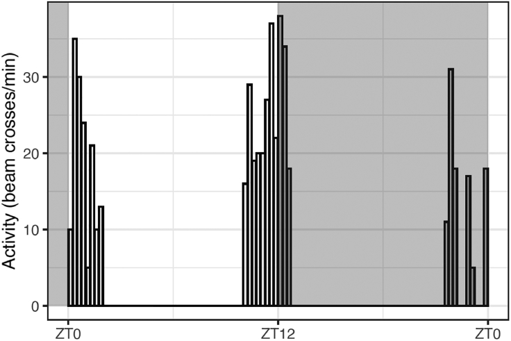
For illustration purposes, we visualize the activity of fly1 by using bars centered at the corresponding bins obtained by seq_along(fly1), set as the x variable (Figure 1). The bars are colored in light or dark gray based on their state value (with fill=state).

Figure 1.

Plot of fly activity on LD5 centered at ZT12

Average activity plots

Timing: 10 min

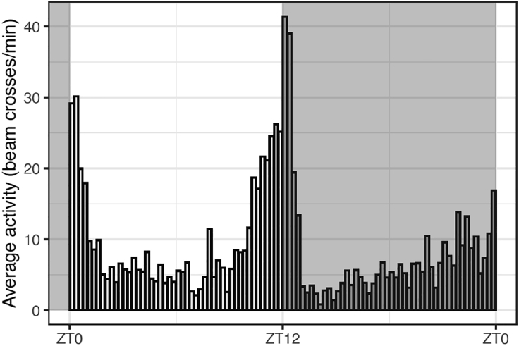
Before computing the row averages to get the average activity plot, dead flies should be removed. We define a fly to be “dead” if it has zero activity in every single bin. In particular, having a non-zero activity in one bin only would classify the fly as “alive.” For details and code used in this step, see Supplemental methods, section 3.3.

• 14.
  Generate average activity plots.

  • a.
    Compute the index vector of all live flies using the live_flyindex() function.
  • b.
    Compute the average activity across all live flies on LD5 by taking row-wise averages.
  • c.
    Create the average activity plot with ggplot(), shown in Figure 2, using the new avg variable inside data that we created in part b.

Figure 2.

The average activity of all live flies on LD5

Smoothing the data

Timing: 30 min

A filter applied on the fly counts removes the high frequencies in the spectrum, i.e., a low-pass filter that smooths out the data.

• 15.Apply a Butterworth filter. For details and the code used in this step, see Supplemental methods, section 3.4.
  The Butterworth filter is a recursive filter of the form:

  $$v_j=\sum _{p=0}^P{a}_p{u}_{j-p}+\sum _{q=1}^Q{b}_q{v}_{j-q}+\sum _{q=1}^Q{b}_q{v}_{j-q}$$

  where $u_j,j=1,\mathrm{...},N$ is the original signal, and $v_j,j=1,\mathrm{...},N$ is the filtered signal. Note that this filter depends not only on the current and the previous $P$original data points, but also on the previously filtered $Q$ points, relative to the current point. Thus, the current filtered value depends not only on a weighted average of the unfiltered values (first sum), but also recursively on the previously computed $Q$ filtered values (second sum). The art of filter design is to compute the values of the $P+1$parameters $a_p,p=0,\mathrm{...},P$and the $Q$ parameters $b_q,q=1,\mathrm{...},Q$ so that the frequency requirements are met. We use a 2nd order low-pass Butterworth filter with $P=Q=2$.
  This filter is causal since it uses only past data and this leads to a phase delay in the filtered data. The phase delay can be removed by additional filtering backward in time.

  • a.
    To compute the Butterworth filter weights, use the function butter() from the signal package.
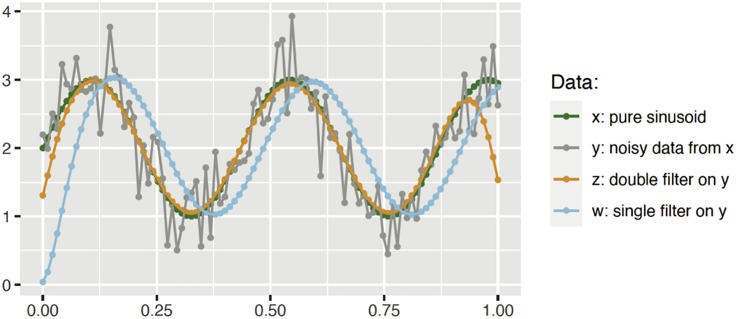
  • b.
    Then, use the function filtfilt(), which applies a linear digital filter twice, once forward and once backward in time. The double filter has zero-phase delay and a filter order twice that of the original. Having a zero-phase delay is essential for the phase computations in the context of fly activity.

Figure 3 shows the results of applying single and double filters to the noisy data generated by a pure sinusoid. The double filter traces very closely the original pure sinusoidal signal used to generate the noisy data, except around the end points. The phase delay of the single filter is also quite clear.

Figure 3.

Single and double Butterworth filters applied to noisy data generated from a pure sinusoid

Obtaining the evening phase of a single fly

Timing: 30 min

A Butterworth filter was applied to smooth out the fly data and compute the evening phase for a single fly using a window centered at 10:00 PM on LD5. For the 15 min bin data the 49th bin was used (first bin in dark state), to represent the evening phase bin relative to which the phase shift was computed. For details and code used in this step, see Supplemental methods, section 3.5.

• 16.
  To generate the Butterworth filter parameters, use the butter() function from the signal R package. The arguments are:

  • •
    n is the filter order. We first explore the data with n=1,2 for a first and second order filter.
  • •
    W is the critical frequency of the filter and it must be a scalar for a low-pass filter. For digital filters, W must be between 0 and 1, where 1 is the Nyquist frequency. We start our explorations with either W=0.1 (10 Hz) or W=0.2 (5 Hz).
  • •
    type is set to “low” for a low-pass filter.
  • •
    plane is set to “z” for a digital filter.
    The function butter() returns an ARMA object with list elements:
  • •
    a, which holds the autoregressive (AR) polynomial coefficients for the recursive part.
  • •
    B, which holds the moving average (MA) polynomial coefficients for the weighted sum part.

• 17.
  Compute the evening phase for a single fly.

  • a.
    In the example provided, we found all peaks in the filtered data using the findpeaks() function from the pracma R package and then found the peak whose time index minimizes the distance from the time index of ZT12. Distance is given as the absolute value of the difference.
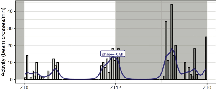
  • b.
    We added to the original data the smoothed data for the single fly, using the mutate() function and applying the double filter filtfilt() to the fly data using the Butterworth filter, described above. Then, we use the findpeaks() function from the pracma R package to find the peak closest to lights off (ZT12). An evening phase value of −0.5 h was obtained for fly18.

Plotting the raw, unfiltered data with the phase value

Timing: 15 min

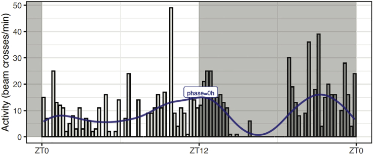
• 18.Use the R function phasePlot()which generates plots like one shown in Figure 4, which includes the raw activity data for fly18. The raw data was smoothed using a first order filter with 5 Hz critical frequency (W=0.2). The filtered data for this particular fly is plotted using a line plot in blue color. Note that the algorithm does not pick the highest peak of activity, but the peak closest to lights off as it can be seen in the case of fly18, where the phase corresponds to the second-highest peak.

Figure 4.

Raw and filtered data for a single fly and its evening phase on LD5 (Figure 6 in supplemental experimental procedures)

For details and code used in this step, see Supplemental methods, section 3.6. For detailed information regarding the full phase sample in LD, see Supplemental methods, section 3.7.

Phase analysis on DD1

Timing: 30 min

For details and code used in this step, see Supplemental methods, section 4 (subsections 4.1 and 4.2)

• 19.Load in RStudio the DD1 data file DD1APm15mCtM016.txt obtained from DAMFileScan111X. Note that the DD1 data are centered at 10:00PM on DD1. The resulting dataframe has 96 observations for the 96 bins covering the 24 h that we have selected, divided into 15 min bins. It has 42 variables, where the last 32 variables (columns) are representing the 32 flies. Table 3 shows the first 12 columns and the first 4 rows of the data. Column 11 (X11) represents the first fly on DD1.

Table 3.

The head of the DD1 data

X1	X2	X3	X4	X5	X6	X7	X8	X9	X10	X11	X12
402780	7 Jul 20	10:15:00	1	14	0	0	0	0	0	27	15
402795	7 Jul 20	10:30:00	1	14	0	0	0	0	0	25	7
402810	7 Jul 20	10:45:00	1	14	0	0	0	0	0	10	0
402825	7 Jul 20	11:00:00	1	14	0	0	0	0	0	23	25

Supplemental methods, Table 4.

Next, we performed the same data processing that we did for the LD5 data. Table 4 shows the first 12 columns and a slice of rows 47:50 around 10:00 PM of our data.

Table 4.

The DD1 data around 10:00PM, showing rows 47:50

Time	state	fly1	fly2	fly3	fly4	fly5	fly6	fly7	fly8	fly9	fly10
21:45	light	20	14	22	18	12	34	13	31	20	17
22:00	light	30	11	38	10	16	27	25	35	27	21
22:15	dark	28	12	20	20	26	37	27	38	20	10
22:30	dark	14	21	0	35	25	21	20	45	25	18

Supplemental methods, Table 5.

Note that the table indicates “light” or “dark” for clarity but this refers to subjective day and subjective night, respectively (free running conditions in Drosophila are constant darkness and constant temperature).

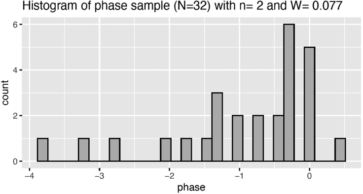
To illustrate, we show in Figure 5 the evening phase obtained for fly2, using the optimal filtering parameters obtained by calibrating the filter to the LD5 data. The distribution of the phase sample on DD1 obtained with optimal filter parameters is show in Figure 6.

Figure 5.

Raw and filtered activity for fly2 and its evening phase on DD1 with optimal filter parameters (Figure 11 in supplemental experimental procedures)

Figure 6.

The frequency histogram of the phase sample on DD1 (Figure 12 in supplemental experimental procedures)

Circular data analysis and visualizations

Timing: 30 min

In this section, we illustrate the circular data analysis (Batschelet, 1981)(Levine et al., 2002, Pewsey et al., 2013) and visualization functionality of the R package circular, which can be installed in RStudio from CRAN. For illustration purposes, we use the actual phase data from our original paper (Fernandez et al., 2020). For details and code used in this step, see Supplemental methods, section 5. A good introduction to the analytical aspects of circular statistics can be found in (Pewsey et al., 2013), and the R package circular is illustrated in (Batschelet, 1981).

Data were obtained from a system entrained to a 24 h environmental cycle (lights on=ZT00). Negative phases represent increased activity (anticipation) before lights on or lights off transitions, thus if a transition was anticipated there would be a negative phase value. On the other hand, the positive phases represent a delay in response relative to ZT00 time set at “midnight” on our clock.

• 20.Import the raw phase data into RStudio. The phases dataframe has 7 variables and 64 observations, including NAs. The variables represent the phases for different genotypes. For details and code used in this step, see Supplemental methods, section 5.1.
• 21.Transform the phases into proper hours by taking the original phases modulo 24, and then converting the hours into radians. For details and code used in this step, see Supplemental methods, section 5.2.

The zero-hour ZT00 is set at 24 h, or $2\pi$ radians. The conversion formula is given by:

$${\varphi }_1=\frac{\left({\varphi }_{0}mod24\right)2\pi }{24}$$

where ${\varphi }_0$is the raw phase, $\left({\varphi }_{0}mod24\right)$ is taking the raw phase modulo 24, which gives a proper hour on the 24 h clock, and ${\varphi }_1$ is the converted angular phase, given in radians. We then need to create a circular data object, using the function circular() from the circular package, which contains the phases as angles measured in radians on a 24 h clock.

We illustrate the application of the Watson-Wheeler Test for Homogeneity of Angles and the Watson Two-Sample Test of Homogeneity to determine whether the phases for control and experimental lines are significantly different. Watson’s non-parametric two-sample statistic $U^2$ provides a criterion to test whether two samples differ significantly from each other. For both tests, the null hypothesis is that the two samples of angles come from the same underlying population.

• 22.Generate circular data plots. Applying the generic plot() function to a circular data object, creates a circular data plot. For details and code used in this step, see Supplemental methods, section 5.3.

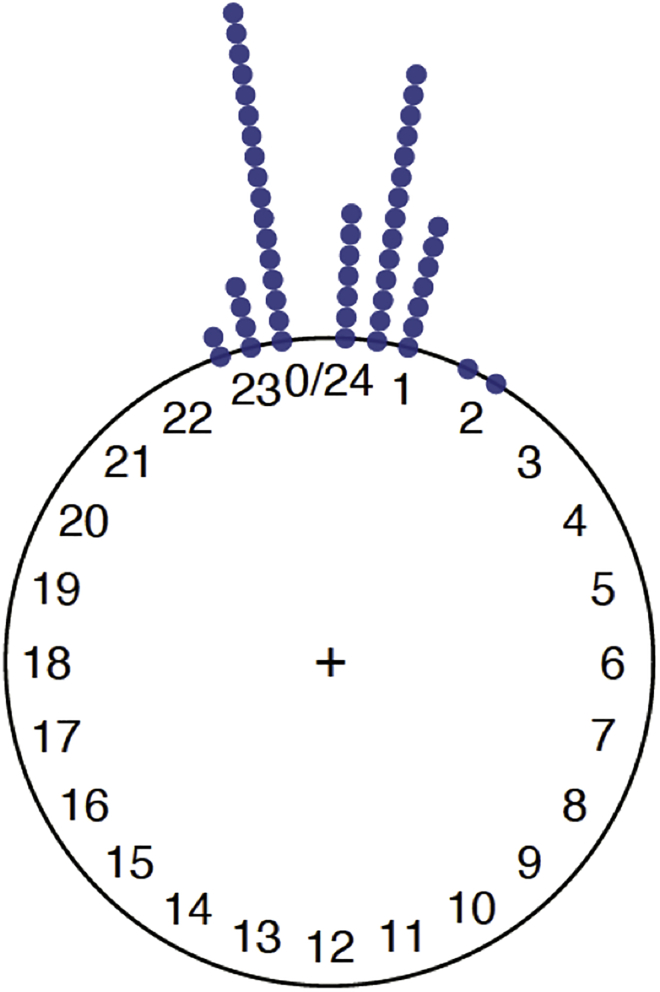
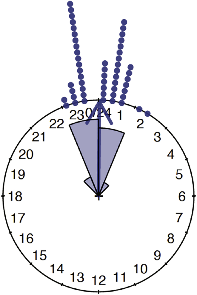
Figure 7 shows the plot for the first phase variable (the genotype PdfGal4) in the circular data object. Inside plot(), the argument stack = TRUE allows for different observations corresponding to the same (or close enough) angle to be stacked on the top of each other.

Figure 7.

Pdf-Gal4 phases in radians (Figure 13 in supplemental experimental procedures)

The circular mean computes the mean direction of a circular variable. Each angular observation in the circular variable is treated as a unit vector, or a point on the unit circle. The resultant vector of all observations is computed and the direction of the resultant vector is returned as the circular mean, which is implemented in the circular package as a method for the generic function mean(), applied to a circular data object.

Since the phase data have NA values, we use the na.rm = TRUE argument to remove the NA values.

Note: NA stands for "not available," and it is a reserved symbol in R used to represent a missing value. For example, the phases corresponding to dead flies would be computed as NAs, because there are no data available for dead flies.

For details and code used in this step, see Supplemental methods, section 5.4.

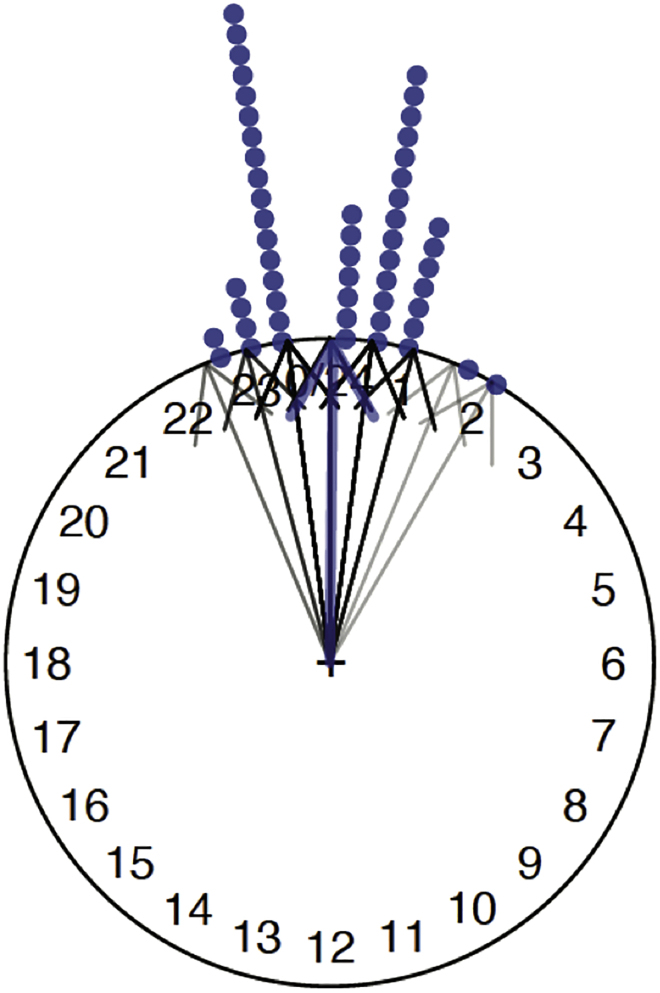
• 23.Visualize the circular mean as the mean direction of a circular variable by plotting an arrow that represents the resultant mean direction vector, using arrows.circular(). The call arrows.circular(data) displays the vectors on the unit circle corresponding to the angles (in radians) in the circular variable data, relative to the zero on the 24 h clock. To display the mean resultant vector, we use the mean resultant length of the circular variable, computed with rho.circular(). This is shown in Figure 8

Figure 8.

Mean direction, shown by the blue arrow (Figure 15 in supplemental experimental procedures)

The rose diagram represents frequencies in the circular data by areas of sectors on the unit circle and can be added to an existing circular plot using the rose.diag() function. For more details on the many arguments this function has, please refer to the circular package documentation. There are two conventions in the literature regarding rose diagrams. Here we use the default convention of the rose.diag() function, where the radius of a segment is taken to be the square root of the relative frequency. With this convention, when we compare segments in a rose diagram, the ratio of the areas of two segments is the same as the ratio of the relative frequencies, since the segment areas are proportional to the radius squared. See the supplement for more details.

• 24.Add a rose diagram to a circular plot as well as an arrow pointing in the mean circular direction of the circular data, as shown in Figure 9. In the rose.diag() function, the argument bins=16 controls the number of segments, and the argument prop=1.1 scales the size of all segments relative to the outer circle, with larger values increasing the size of the segments, having a default value of one. For details and code used in this step, see Supplemental methods, section 5.5.

Figure 9.

Mean direction vector (in blue), and a rose diagram of PdfGal4 (Figure 16 in supplemental experimental procedures)

Expected outcomes

The Watson two-sample test can be applied to determine whether the phases for control and experimental lines are significantly different. For details and code used in this step, see Supplemental methods, section 5.6.

Watson’s non-parametric two-sample $U^2$ statistic provides a criterion to test whether two samples differ significantly from each other. The circular data should consist of two independent random samples of circular observations drawn from populations with a continuous distribution. The null hypothesis $H_0$ states that the two samples belong to the same parent population.

The decision rule states that:

• •If $U^2<$ critical value: the null hypothesis cannot be dismissed.
• •If $U^2>$ critical value: reject the null hypothesis and conclude that the two samples differ significantly.

The Watson two-sample test for homogeneity can be used on two or more samples of circular data, using the function watson.twotwo.test(). The difference between the samples can be in either the mean or the variance. The p-value is estimated by assuming that the test statistic follows a chi-squared distribution. For this approximation to be valid, each dataset must have at least 10 elements. The alpha argument of this function specifies the significance level of the test. Valid levels are 0.001, 0.01, 0.05, 0.1. This argument can be omitted, in which case, a range for the p-value will be returned.

One can also apply the Watson-Wheeler test for homogeneity on two or more samples of circular data, using the function watson.wheeler.test() from the circular package. The difference between the samples can be in either the mean or the variance.

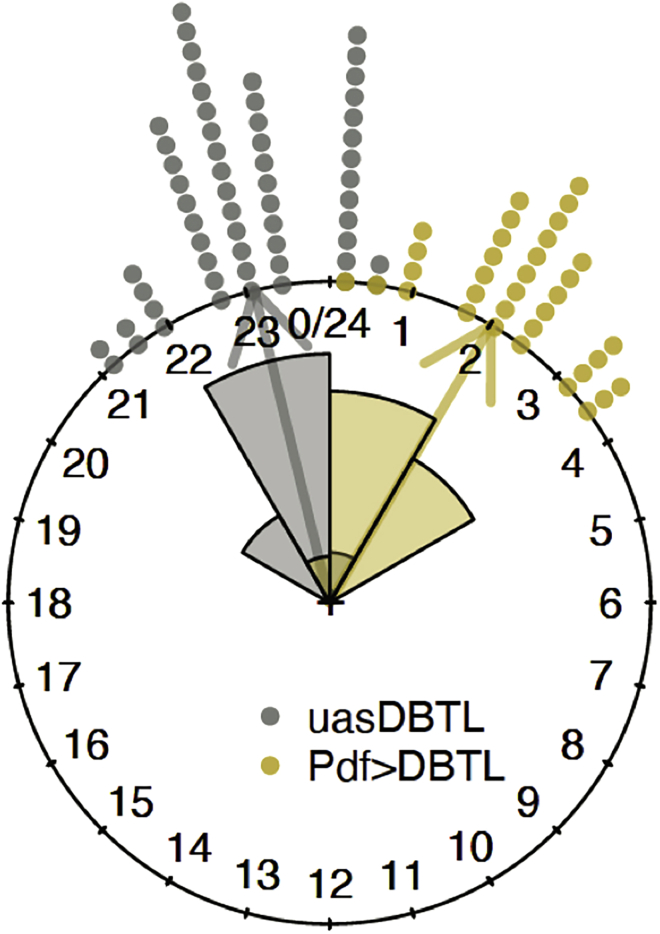
• 25.Create the circular plot of uasDBTL and PdfDBTL, along with arrows pointing to the circular means of the two datasets, and their rose diagrams, shown in Figure 10. For details and code, see Supplemental methods, section 5.7.

Figure 10.

The circular plot and rose diagrams of uasDBTL and PdfDBTL (Figure 17 in supplemental experimental procedures)

Limitations

A more complex definition of a “dead fly” may be needed for the average activity plot, which accounts for flies that can be considered “dead” even though they may have some non-zero activity within a given time interval. Additionally, it may be required to optimize the filter calibration for speed if applied to large data, and if used to create a Shiny App running on a RStudio server. Further, it may be useful to add a function that creates an average activity plot across any given range of LD days that can be used for filter calibration.

Troubleshooting

Problem 1

A lack of behavior tracking to temperature ramp cycles by control flies, caused by overcrowded incubators and low humidity levels.

Potential solution

For better entertainment conditions we suggest limiting the number of monitors per incubator to a maximum of 10, if using Percival models. We also suggested adding a tub of water to the bottom of each incubator to control for humidity. We predict that overcrowding the incubator prevents each individual fly tube to heat up to the fullest expression, making it hard for the flies to properly entrain to these conditions.

Problem 2

A high percentage of F1 flies that die during the experimental run.

Potential solution

This problem has multiple possible solutions. The first is to limit the flies’ exposure to CO₂, as overexposure to CO₂ is lethal to the flies. When loading the flies try to minimize the time they spend on the fly pad, the maximum time is 10 min. The second solution is to ensure there is enough food in the vials and it is properly made to sustain the flies for 20 days. Finally, ensure the flies you load are young and healthy. If environmental monitors were used, check to make sure unprogrammed changes in temperature were not responsible for killing flies.

Resource availability

Lead contact

Further information and requests for resources and reagents should be directed to and will be fulfilled by the Lead Contact, Maria P. Fernandez (mfernand@barnard.edu).

Materials availability

All unique/stable reagents generated in this study are available from the lead technical contact and the corresponding author without restriction. Further information and requests for resources and reagents should be directed to and will be fulfilled by Maria P. Fernandez and Boyan Kostadinov.

Data and code availability

TheGitHub repository contains the RMarkdown (Rmd) source document with the code used for all computations and visualizations discussed in the paper. For a full reproducibility, it also contains the data files used in the source Rmd document. We use theR programming environment and theRStudio IDE for all data analysis and visualizations.

References

- Abhilash L., Sheeba V. RhythmicAlly: Your R and shiny–based open-source ally for the analysis of biological rhythms. J. Biol. Rhythm. 2019;34:551–561. doi: 10.1177/0748730419862474. [DOI] [PubMed] [Google Scholar]
- Batschelet E. Academic Press; 1981. Circular statistics in biology. [Google Scholar]
- Chyb S., Gompel N. Academic Press; 2013. Atlas of Drosophila morphology : wild-type and classical mutants. [Google Scholar]
- Fernandez M.P., Pettibone H.L., Bogart J.T., Roell C.J., Davey C.E., Pranevicius A., Huynh K.V., Lennox S.M., Kostadinov B.S., Shafer O.T. Sites of circadian clock neuron plasticity mediate sensory integration and entrainment. Curr. Biol. 2020;30:2225–2237.e5. doi: 10.1016/j.cub.2020.04.025. [DOI] [PMC free article] [PubMed] [Google Scholar]
- Geissmann Q., Garcia Rodriguez L., Beckwith E.J., French A.S., Jamasb A.R., Gilestro G.F. Ethoscopes: An open platform for high-throughput ethomics. PLoS Biol. 2017;15:e2003026. doi: 10.1371/journal.pbio.2003026. [DOI] [PMC free article] [PubMed] [Google Scholar]
- Helfrich-Forster C., Winter C., Hofbauer A., Hall J.C., Stanewsky R. The circadian clock of fruit flies is blind after elimination of all known photoreceptors. Neuron. 2001;30:249–261. doi: 10.1016/s0896-6273(01)00277-x. [DOI] [PubMed] [Google Scholar]
- Keleman K., Dickson B.J. Short- and long-range repulsion by the Drosophila Unc5 netrin receptor. Neuron. 2001;32:605–617. doi: 10.1016/s0896-6273(01)00505-0. [DOI] [PubMed] [Google Scholar]
- Levine J.D., Funes P., Dowse H.B., Hall J.C. Signal analysis of behavioral and molecular cycles. BMC Neuroscience. 2002;3:1. doi: 10.1186/1471-2202-3-1. [DOI] [PMC free article] [PubMed] [Google Scholar]
- Muskus M.J., Preuss F., Fan J.-Y., Bjes E.S., Price J.L. Drosophila DBT lacking protein kinase activity produces long-period and arrhythmic circadian behavioral and molecular rhythms. Mol. Cell. Biol. 2007;27:8049–8064. doi: 10.1128/MCB.00680-07. [DOI] [PMC free article] [PubMed] [Google Scholar]
- Park J.H., Helfrich-Forster C., Lee G., Liu L., Rosbash M., Hall J.C. Differential regulation of circadian pacemaker output by separate clock genes in Drosophila. Proc. Natl. Acad. Sci. U S A. 2000;97:3608–3613. doi: 10.1073/pnas.070036197. [DOI] [PMC free article] [PubMed] [Google Scholar]
- Pewsey A., NeuhäUser M., Ruxton G.D. Oxford University Press; 2013. Circular statistics in R. [Google Scholar]
- Pfeiffenberger C., Lear B.C., Keegan K.P., Allada R. Locomotor activity level monitoring using the Drosophila Activity Monitoring (DAM) System. Cold Spring Harb. Protoc. 2010;2010 doi: 10.1101/pdb.prot5518. pdb prot5518. [DOI] [PubMed] [Google Scholar]
- Pfeiffenberger C., Lear B.C., Keegan K.P., Allada R. Processing circadian data collected from the Drosophila Activity Monitoring (DAM) System. Cold Spring Harb. Protoc. 2010;2010 doi: 10.1101/pdb.prot5519. pdb prot5519. [DOI] [PubMed] [Google Scholar]
- Renn S.C.P., Park J.H., Rosbash M., Hall J.C., Taghert P.H. A pdf neuropeptide gene mutation and ablation of PDF neurons each cause severe abnormalities of behavioral circadian rhythms in Drosophila. Cell. 1999;99:791–802. doi: 10.1016/s0092-8674(00)81676-1. [DOI] [PubMed] [Google Scholar]
- Schmid B., Helfrich-Forster C., Yoshii T. A new ImageJ plug-in "ActogramJ" for chronobiological analyses. J. Biol. Rhythms. 2011;26:464–467. doi: 10.1177/0748730411414264. [DOI] [PubMed] [Google Scholar]
- Wickham H., Grolemund G. O'Reilly; 2016. R for data science : import, tidy, transform, visualize, and model data. [Google Scholar]
- Yao Z., Bennett A.J., Clem J.L., Shafer O.T. The Drosophila clock neuron network features diverse coupling modes and requires network-wide coherence for robust circadian rhythms. Cell Rep. 2016;17:2873–2881. doi: 10.1016/j.celrep.2016.11.053. [DOI] [PMC free article] [PubMed] [Google Scholar]
Associated Data
This section collects any data citations, data availability statements, or supplementary materials included in this article.
Supplementary Materials
Data Availability Statement