To Adjust or Not to Adjust? When a “Confounder” Is Only Measured After Exposure

Supplemental Digital Content is available in the text.

Abstract

Advice regarding the analysis of observational studies of exposure effects usually is against adjustment for factors that occur after the exposure, as they may be caused by the exposure (or mediate the effect of exposure on outcome), so potentially leading to collider stratification bias. However, such factors could also be caused by unmeasured confounding factors, in which case adjusting for them will also remove some of the bias due to confounding. We derive expressions for collider stratification bias when conditioning and confounding bias when not conditioning on the mediator, in the presence of unmeasured confounding (assuming that all associations are linear and there are no interactions). Using simulations, we show that generally neither the conditioned nor the unconditioned estimate is unbiased, and the trade-off between them depends on the magnitude of the effect of the exposure that is mediated relative to the effect of the unmeasured confounders and their relations with the mediator. We illustrate the use of the bias expressions via three examples: neuroticism and mortality (adjusting for the mediator appears the least biased option), glycated hemoglobin levels and systolic blood pressure (adjusting gives smaller bias), and literacy in primary school pupils (not adjusting gives smaller bias). Our formulae and simulations can inform quantitative bias analysis as well as analysis strategies for observational studies in which there is a potential for unmeasured confounding.

In observational epidemiologic studies, often the interest lies in the causal effect of an exposure on a certain outcome, yet this may be biased by (unmeasured) confounding.¹ To control for confounding, generally, it is advised to condition on (a sufficient set of) confounders, that is, variables that cause both exposure and outcome.^2–5 Textbooks on epidemiology, as well as research articles about confounding adjustment, generally advise against controlling for variables that are measured after exposure has started.^6–12 One reason is that adjustment for postexposure variables may lead to collider stratification bias. Another reason is that such variables may actually be mediators of the causal relationship between exposure and outcome, and conditioning on such variables may introduce bias.^5,13 As indicated by VanderWeele: “…we often refrain from adjusting for covariates that occur temporally subsequent to the exposure.”³

Nevertheless, in applied research, postexposure variables are sometimes adjusted for in the analysis of an observational study. For example, in a cohort study of the effect of prevalent vitamin K antagonist use on renal function, adjustment was made for measurements of hemoglobin and glomerular filtration rate at cohort entry (i.e., after initiation of vitamin K antagonist use).¹⁴ In a case–control study of very hot tea consumption and esophageal cancer, adjustment was made for the confounder “oral hygiene” measured at the time of outcome assessment.¹⁵ In another case–control study of migraine and the risk of stroke, adjustment was made for several confounders, again measured at the time of outcome assessment.¹⁶ One may wonder whether these are examples of bad practice or whether there could be instances in which adjustment for a postexposure variable could, in fact, be beneficial, particularly if the postexposure variable may carry information about unmeasured confounders.

Bias formulas for unmeasured confounding have been described, for example, in Arah et al¹⁷ and Vanderweele and Arah.¹⁸ However, these do not consider scenarios where a variable related to an unmeasured confounder may also be caused by the exposure. Here, we consider that scenario where an effect of the exposure, or a mediator, is associated with an unmeasured confounder and derive expressions for the bias when conditioning and when not conditioning on the mediator. The use of these formulae is illustrated by three examples: a study of neuroticism and mortality, a study of glycated hemoglobin levels and systolic blood pressure (SBP), and a study of literacy in primary school pupils.

METHODS

Notation and Setup

To derive expressions for the bias due to unmeasured confounding and the bias due to conditioning on a mediator that is (possibly) associated with an unmeasured confounder, we consider the model depicted in Figure 1. X denotes the exposure, Y the outcome of interest, and M is a mediator of the effect of X on Y. The variables U₁ and U₂ are unmeasured variables. U₁ is a confounder of the -relation, and U₁ also causes M. U₂ is a confounder of the -relation, but not of the -relation. Each variable is a linear combination of the variables affecting it (indicated by the directed arrows in Figure 1) plus an error term. We assume there are no interactions between variables in their effects on outcome or mediator. Furthermore, we assume that all variables are normally distributed, all associations are linear and additive, all errors uncorrelated, and there is no interaction between variables. The regression coefficients of the linear models are denoted by , for example,  for the effect of X on M. The variances of the errors are denoted by , for example, for the variance of the error of Y. We assume an ordinary least squares (OLS) estimator is used to obtain estimates of the relation between exposure and outcome. Furthermore, we assume no other sources of bias (no model misspecification, no measurement error, and no missing data).¹⁹ We note that under the model depicted in Figure 1, the causal effect of X on Y is in principle not identifiable, due to U₁ and U₂ being unmeasured (in the eAppendix, http://links.lww.com/EDE/B760; we provide an explanation for this based on a single-world intervention graph, or SWIG).²⁰

Figure 1.

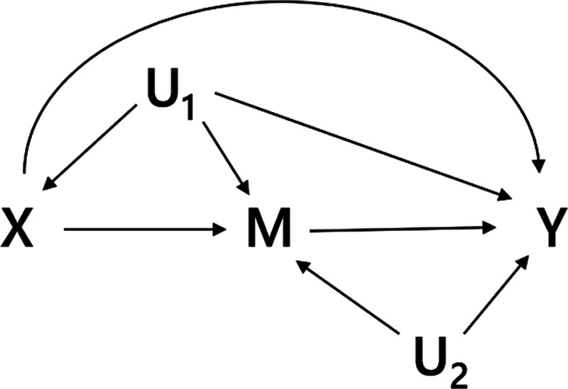
Directed acyclic graph of an exposure (X), an outcome (Y), a mediator (M), and two unmeasured variables (U₁ and U₂).

We have written an app demonstrating the biases described in the paper, which is available at https://remlapmot.shinyapps.io/bias-app/. The source code for the app is on GitHub at https://github.com/remlapmot/bias-app.

Bias Due to an Unmeasured Confounder

Here, we derive expressions for the scenario depicted in Figure 1, where both U₁ and U₂ are considered to be unmeasured (details about the derivations of the bias expressions are presented in the eAppendix; http://links.lww.com/EDE/B760). When U₁ is unmeasured, this variable cannot be adjusted for and the estimator of the total effect of X on Y will be biased. The (true) total effect of X on Y is given by . Using the path tracing rules, the observed relation between X and Y is, in expectation,

(1)

Here, is the direct effect of X on Y, the direct effect of M on Y, etc. The bias in the OLS estimator of the total effect of X on Y is given by

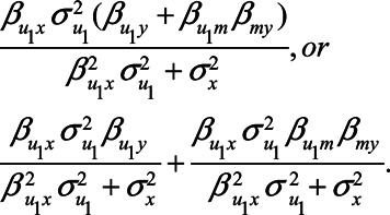The two components of this second expression represent the two back-door paths from X to Y: the first term represents the path and the second term represents the path . Note that if U₁ does not cause X (), then there is no bias due to unmeasured confounding. If U₁ does not cause Y directly (i.e., ), then there is a nonzero bias due to unmeasured confounding that is mediated by M.

Expression (1) can be simplified when assuming all error terms are equal to 1 (i.e., , ). Then

If the unmeasured confounder does not cause the mediator, that is, , this bias expression simplifies to .

Bias due to conditioning on a mediator

To explore under what scenarios conditioning on M may remove (part of) the confounding effect by U₁, we derive an expression for the OLS estimator of the relation between X and Y, when conditioning on M. Derivations of the general expressions are presented in the eAppendix; http://links.lww.com/EDE/B760. For clarity, here we assume all error terms are equal to 1 (i.e., , , etc.). In that case, conditioning on M is expected to result in the observed relation between X and Y to be

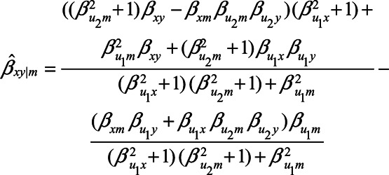(2)

When , expression (2) reduces to

which reduces even further to

if the unmeasured confounder U₁ does not cause the mediator M, that is, when . When , yet , expression (2) reduces to

If we assume no unmeasured confounding by U₁, for example, because , this reduces further to

Even though there is no unmeasured confounding of the -relation by U₁, clearly this expectation of the observed relation between X and Y differs from the total effect of X on Y (), which is partly due to blocking of the direct effect of X on Y via M and partly due to collider stratification bias (opening the path ).

The bias expressions were supported by statistical simulations. Details of these simulations and their results are presented in the eAppendix; http://links.lww.com/EDE/B760.

Illustration of Bias Formulas

To illustrate the use of the bias formulae (1) and (2), we first present a numerical example. The bias formulae can be applied by specifying the parameters. First, we could assume all the error terms (, , , , and ) are equal to 1. Next, based on the literature or own experience the other parameters could be specified. For example, we could assume that a one-unit increase in the unmeasured variable U₁ causes an increase in each of X, M, and Y of 0.3 (). Likewise, we could assume that a one-unit increase in the unmeasured variable U₂ causes an increase in each of M and Y of 0.2 (). Also, we assume that a one-unit increase in X causes and increase in M of 0.4 () and that a one-unit increase in M causes an increase in Y of 0.7 (). Finally, we assume that X has no direct effect on Y (i.e., ). With these numbers, we can apply the bias formulae and calculate the bias. Without adjustment for U₁, the bias in the estimated relation is , whereas with adjustment for U₁, the bias is .

Figure 2 illustrates the impact of various model parameters on the bias of the OLS estimator of the relation due to unmeasured confounding by U₁, with and without adjustment for the mediator M. These results are based on expressions (1) and (2). Specifically, the values of error terms (, , , , and ) were set to 1. The value of the model coefficients (, , , , , , and ) were each set to or 1.00, while was set to 0. This means that in total 78,125 different configurations of the parameter values were investigated. In each panel, the bias is plotted against the variation in one of the parameters. The distribution of the bias (represented as a boxplot) is due to the variation in the other parameter; that is, each is marginal over the values of the other parameters.

Figure 2.

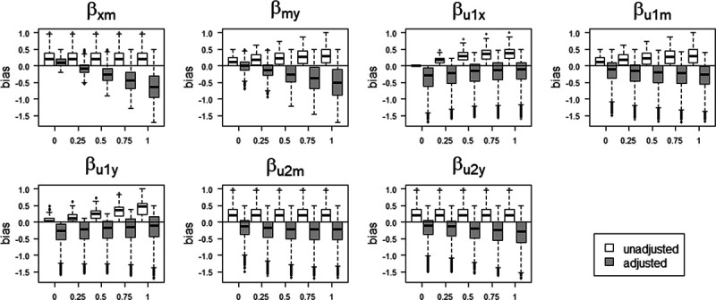
Bias in the OLS estimator of the X  – Y relation when conditioning on a mediator (adjusted) and when omitting a mediator (unadjusted), when the mediator is caused by an unmeasured confounder. The distribution of bias values for each parameters is marginal over the values of the other parameters. OLS, ordinary least squares.

The figure shows situations when conditioning on a mediator may actually lead to a larger bias, compared with not conditioning on a mediator, for example, when the indirect effect via M becomes larger (indicated by increasing values of and ). Particularly when and have larger values, adjustment may be preferred, however those settings do include scenarios in which adjustment can lead to a relatively large negative bias. For the parameters and , both approaches tend to result in bias, although adjustment for the mediator M can result in bias that is larger in magnitude, owing to collider stratification bias. Note that in this illustration, all parameters of the bias formulae have a zero or positive value. However, if, for example, we take the same parameter values as mentioned above (i.e., ),   but set and to negative values (i.e., , then the bias after adjustment for the mediator would be positive (0.25) whereas not adjusting would result in a negative bias (−0.14).

Example 1—Neuroticism and Mortality

To illustrate the use of the expressions for bias, presented in the previous sections, we consider a study of the relation between neuroticism and mortality risk, in which neuroticism and self-rated health were measured at cohort entry.²¹ In this case, self-rated health scores could have been affected by preexisting neuroticism, yet at the same time could be related to unmeasured health status (see Figure 3 for a graphical representation). Conditioning on self-rated health scores may control for confounding but may also induce a bias due to conditioning on the mediator. In this situation, the data analyst needs to identify whether the bias introduced by conditioning on the mediator is likely to be greater than the bias introduced by not conditioning on it. This assessment could inform the analysis strategy.

Figure 3.

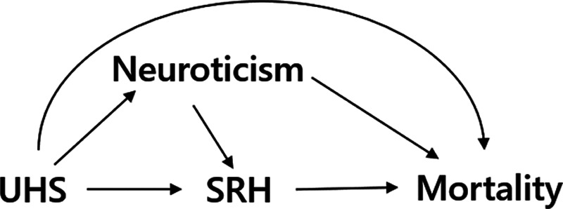
Directed acyclic graph of example 1: the relation between neuroticism and mortality, with UHS being a confounder and SRH a mediator. SRH, self-rated health; UHS, unmeasured health status;

In terms of the model presented in the previous section, X would represent neuroticism, Y mortality, M self-rated health score, and U₁ would represent unmeasured health status. For brevity, we assume there is no confounding of the relation by a variable U₂. If we assume that there is no direct effect of self-rated health on mortality, but only indirectly via health status, we set and remove the arrow from self-rated health to mortality from the graph. Furthermore, we assume for ease of interpretation that the effect of X on M is equal to the effect of U on M and that the effect of U on X is equal to the effect of U on Y.²² In addition, all error terms () were set to 1.

Figure 4 shows the difference in absolute bias of not conditioning on self-rated health score versus conditioning on self-rated health score for various scenarios. In those scenarios in which the confounding effect of U₁ is relatively small (), both analytical approaches give small bias. However, when the confounding effect is larger, differences are more pronounced. If the unmeasured confounder is positively associated with X and Y (e.g., ), adjustment for M reduces the bias. In contrast, if the unmeasured confounder is negatively associated with X and Y (), adjustment for M leads to an increase in bias. The reason for the latter phenomenon is collider stratification bias: upon adjustment for M, the relation between U₁, and X becomes stronger, thus increasing the confounding effect by U.

Figure 4.

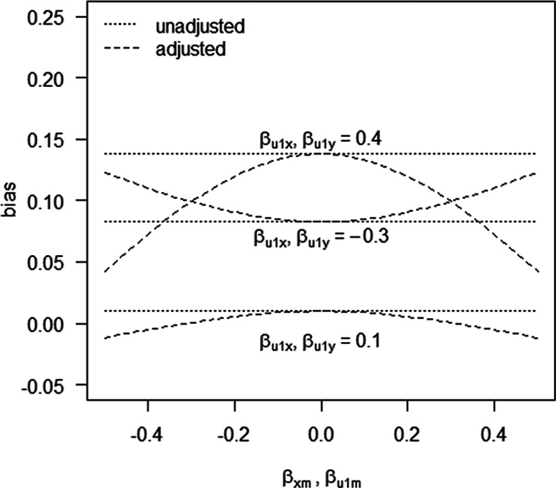
Bias in example 1 when conditioning on a mediator (adjusted) and when omitting a mediator (unadjusted), when the mediator is caused by an unmeasured confounder. See main text for details.

Arguably, a more realistic scenario is that in which neuroticism has a negative effect on self-rated health (e.g., ), while health status has a positive effect on self-rated health (e.g., ). Furthermore, the health status could be negatively associated with neuroticism and mortality (e.g., , and ). Given these values, without adjustment for the health status the bias in the effect of neuroticism is expected to be 0.08. However, when adjusting for self-rated health, this bias is expected to be −0.03. This suggests that, in this scenario, adjustment for self-rated health gives a smaller bias. Although the actual values of the different parameters will be context-specific, an analysis like this may guide data analysts in decisions about analysis strategies and sensitivity analyses of adjustment for a mediator that is caused by an unmeasured confounder, in this case self-rated health scores. Further work could include using more realistic values for the coefficients, if these could be obtained for example from external data or expert opinion.

Example 2—Glycated Hemoglobin Levels and Systolic Blood Pressure

Suppose an interested reader finds an article that describes a study of the relation between glycated hemoglobin levels (HbA1C) and SBP. This relation is estimated using linear regression. Age, sex, and body mass index (BMI) are included as covariates in the model to adjust for confounding. In this cohort study, BMI was measured 2 months after HbA1C levels were measured, for example, because routine data from general practitioners were used. The reader wonders whether the researchers actually should have adjusted for BMI, or if this could ‘adjust away’ part of the effect of HbA1C on SBP. Therefore, she decides to conduct a sensitivity analysis.

Based on the literature and her own experience, she expresses possible ranges of the relations between pre-HbA1c-measurement BMI (), HbA1C, post-HbA1c-measurement BMI (), and SBP (Figure 5). As in the previous example, all error terms (’s) are assumed to be 1 and U₂ is considered absent. For each relation, the possible range is then split in 10 equidistant values. For each of the 100,000 combinations of the values of the five relations, the possible bias due to conditioning on (the mediator that is related to the unmeasured confounder ) is compared with the possible bias due to omitting the unmeasured confounder .

Figure 5.

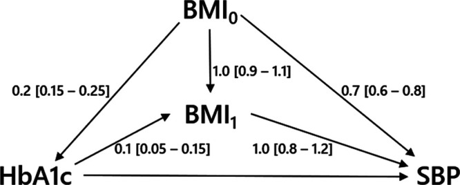
Directed acyclic graph of example 2 with hypothetical values of the relations between , , HbA1C, and SBP. BMI, body mass indexl; SBP, systolic blood pressure.

Figure 6 shows the relative bias of conditioning versus not conditioning on , which indicates that in of the scenarios it would be better not to condition on . In the large majority of scenarios (), however, conditioning on is to be preferred. Based on the assumptions made and the quantification of the bias under two analytical strategies, the reader concludes that she agrees with the choices made by the researchers regarding the analysis of the study of the relation between HbA1C and SBP.

Figure 6.

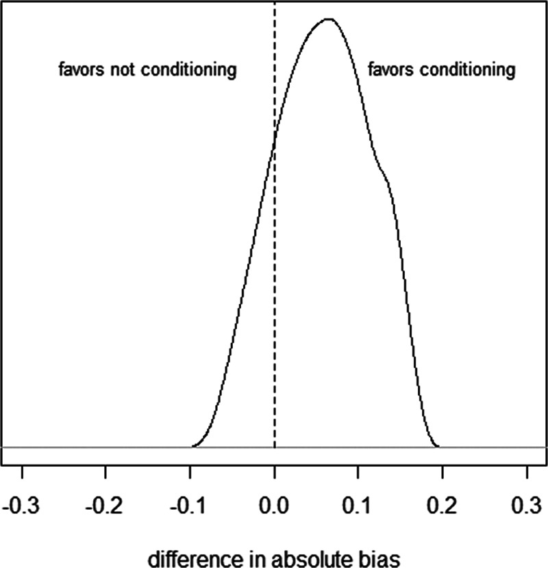
Histogram of difference in absolute bias of conditioning vs. not conditioning on a mediator to control for unmeasured confounding in example 2. Scenarios to the left of the dashed line favor not conditioning on , scenarios to the right of the dashed line favor conditioning on . See main text for details. BMI, body mass index.

Note that different values of the parameters can give rise to the same difference in absolute bias. For example, when have values 0.90, 0.15, 0.17, 1.0, and 0.80, respectively, the difference in absolute bias between adjusting and not adjusting for is approximately zero. Also, when , , , , and have values 1.06, 0.106, 0.172, 1.10, and 0.60, respectively, the difference in absolute bias is approximately zero. However, the magnitude of the bias differs: 0.13 for the first scenario and 0.10 for the second scenario. Furthermore, in both scenarios the bias when not conditioning has a positive sign, whereas the bias when conditioning on the mediator has a negative sign. An alternative approach, like in example 1, would be to consider the (absolute) bias in each of the analytical approaches, instead of their difference; if the bias for both approaches is considered too large, it might be preferable not to conduct a statistical analysis at all but instead put effort in collecting additional data, for example, on U₁ (in this example ).

Example 3—Literacy in Primary School Children

Literacy achievements among primary school pupils may affect their literacy later in life. Suppose researchers are interested in the effect of literacy in the first year of school on literacy 2 years later (i.e., in the third year in school). Literacy is measured in the first and in the third year by means of the Word Recognition and Phonic Skills Test (WRAPS). Age, sex, and phonological capacity may be confounders of this relation. The latter could be measured using the phonological assessment battery (PHAB). For this example, we use data from the ready to learn randomized controlled trial.²³ We use the data of 132 children who received the control intervention, with complete information about WRAPS in years 1 and 3, PHAB in years 1 and 2, age, and sex. These data are available via http://reshare.ukdataservice.ac.uk/853287/, where more information can be found, for instance about ethical review of this study.

We estimated that the relation between WRAPS at baseline and WRAPS after 2 years of follow-up was estimated using linear regression. We included age and sex as covariates in the model to adjust for possible confounding. First, we considered the situation in which a measurement of the confounder PHAB in year 1 is available (reference scenario). After adjustment for age, sex, and PHAB in year 1, we estimated a one-unit increase in WRAPS in year 1 to increase WRAPS in year 3 by 0.70 units (95% CI = 0.43 to 0.97). Next, we assumed that the measurement of the confounder PHAB in year 1 is not available. In this case, after adjustment for only age and sex, we estimated a one-unit increase in WRAPS in year 1 to increase WRAPS in year 3 by 0.74 units (95% CI = 0.48 to 1.00). If, however, a measurement of PHAB in year 2 was available, we could adjust for that, because PHAB in year 2 is probably correlated to PHAB in year 1. After adjustment for age, sex, and PHAB in year 2, we estimated a one-unit increase in WRAPS in year 1 to increase WRAPS in year 3 by 0.63 units (95% CI = 0.37 to 0.88).

In this case, the data allow for estimation of the parameters of the bias formulae (1) and (2), where we assume there is no U₂ and X represents WRAPS in year 1, Y represents WRAPS in year 3, U₁ represents PHAB in year 1, and M represents PHAB in year 2. Based on the estimates of the parameters, conditional on age and sex, we can attribute the following values (rounded to two decimal points) to the parameters: . Given these values, without adjustment for the unmeasured confounder (U₁ /PHAB in year 1) we expect the bias in the effect of WRAPS to be 0.04, which corresponds to the difference in estimates of 0.70 versus 0.74. However, when adjusting for the mediator (M/PHAB in year 2), this bias is expected to be −0.07. This value corresponds to the difference in estimates of 0.70 versus 0.63.

In practice, data would not be available to estimate all parameters. However, estimates may be obtained from analysis of other data sources or retrieved from other source of information. These could then inform a sensitivity analysis.

DISCUSSION

In the presence of unmeasured confounding, conditioning on a mediator that is caused by an unmeasured confounder may reduce, but could also amplify, the bias in the OLS estimator of the exposure-outcome relation. In this paper, we provided expressions for the bias in the OLS estimator for this particular situation to provide support in choosing between two potentially biased estimators. Using simulations, we show that generally neither the conditioned or the unconditioned estimate is unbiased, and the trade-off between them depends on the magnitude of the effect of the exposure that is mediated relative to the confounding effect of the unmeasured confounders and their relations with the mediator.

Epidemiologists are increasingly seeing the value of quantitative bias analysis, whereby statistical formulae and external knowledge are used to estimate the potential size and direction of bias (e.g., due to unmeasured confounding) for a given analysis.^22,24–27 Previous work on the impact of conditioning on a mediator or omitting a confounder already provided expressions for the bias in case of a linear model.^4,13,28–31 We extended this work by considering the situation where a mediator is caused by an unmeasured confounder. In general, neither of the two approaches considered (i.e., conditioning and not conditioning on the mediator) yields an unbiased estimator. Where others considered similar scenarios, yet focused on estimation of indirect effects,^32,33 our interest lay in estimation of the total effect of the exposure on the outcome (and possible bias thereof).

Texts on confounding adjustment generally advise against adjustment for variables that are caused by exposure.^{6,5,12,34–37} Variables measured after initiation of exposure may be caused by (prior) exposure status and therefore are generally not adjusted for.³ Nevertheless, there are several examples of observational studies where adjustment is made for variables that are measured after exposure started, with the aim to control for confounding. To allow for a fair assessment of the quality of an observational study of causal effects, researchers should report relevant details about the timing of the measurement of confounders. If these are measured after the start of exposure, ideally researchers should explain whether they think the measured value represents a mediator or whether it should be considered to hold information about one or multiple unmeasured confounders.³⁸ Directed acyclic graphs may be helpful to support and explain the arguments.³⁹

The expression for the bias when conditioning on the mediator, equation (2), also provides further insight in collider stratification bias. Particularly, if we assume , and are zero, the expression reduces to . In this case, the total effect of X on Y is zero and is the bias due to conditioning on the collider M. Collider stratification bias can arise, for example, due to selective inclusion of subjects into a study or due to missing data.⁴⁰ To quantify the potential bias due to collider stratification, bias expressions like the one presented in this paper could be used.³⁰

Although the linear model allows us to derive expressions for the bias of the different OLS estimators, an obvious limitation is that the results only apply to a limited number of settings. In particular, we have assumed that all associations are linear, and that there are no interactions. Also, the model considered is a gross simplification of what an observational study looks like in reality. In future work, the presented expressions could be extended to more complex models, including nonlinear models. For example, future work could extend the theorems about collider bias for binary outcome models.^41,42 Also, extensions could be considered that take possible correlation between measured and unmeasured confounders into account.^38,43 While we focused on bias in studies with a so-called point-exposure, many exposures are in fact time-varying (neuroticism in the first example is actually more of a time-varying exposure than a point-exposure). Future research could extend our bias formulae to setting of time-varying exposure. We note, however, that our bias expressions already could provide some insight into that situation, by considering the exposure (X) and the mediator (M) as different measurements of exposure (e.g., X₁ and X₂). The expressions could then help to quantify the potential impact of (time-varying) confounding and for example support decisions about the frequency with which time-varying confounders are measured.

An alternative to using bias expressions to guide choices regarding data analysis and to inform sensitivity analysis is to use simulated data to assess bias.^24,25 There are functions in several structural equation modeling packages, which allow the user to generate data from a specified DAG/model. For example, the simulateSEM() function in the dagitty package, the simulateData() function in the lavaan package,^44,45 and functions in the simMixedDAG package.⁴⁶ The user can then fit various proposed models to the data to assess the potential bias in their proposed modeling approach. A simulation approach was also used to assess the likely magnitude of collider bias as an explanation for the obesity paradox.³⁷ And this web application, http://watzilei.com/shiny/collider/, uses simulated data to investigate collider bias for user-specified models.⁴⁷ Additionally, the tipr package implements methods to assess the sensitivity of regression results to unmeasured confounders.^48,49 The expressions presented in this paper offer a relatively simple first approach as compared to more advanced simulation based sensitivity analysis.

In summary, one of the major drawbacks of observational epidemiology is the possibility of unmeasured confounding. Where possible mediators of the exposure-outcome relation hold information about unmeasured confounders, it is important to estimate the bias incurred by both adjusting and not adjusting for these mediators. The bias expressions presented here are helpful to support choices regarding analysis strategies and to inform sensitivity analyses for observational studies in which there is a potential for unmeasured confounding. The result of such a sensitivity analysis could be that collecting data on currently unmeasured confounders is deemed necessary or the study should be stopped because the risk of bias is considered too large. Alternatively, the results of both analyses (adjusted and notadjusted for the mediator) could be presented and the bias expressions presented here could support discussions about the validity of each of the two analyses. Given that there will usually be uncertainty about the values of the parameters, it is not recommended to present the results of just one of the two analyses without acknowledging that uncertainty. Also, we would like to caution against interpreting our results as evidence that adjustment for postexposure variables is advantageous. Instead, we hope they will be the basis of thoughtful investigations of the validity of observational research.

REFERENCES

- 1.Hernán MA, Robins JM. Causal Inference: What If. 2020Boca Raton, FL: Chapman & Hall/CRC; [Google Scholar]
- 2.VanderWeele TJ, Shpitser I. A new criterion for confounder selection. Biometrics. 2011;67:1406–1413. [DOI] [PMC free article] [PubMed] [Google Scholar]
- 3.VanderWeele TJ. Principles of confounder selection. Eur J Epidemiol. 2019;34:211–219. [DOI] [PMC free article] [PubMed] [Google Scholar]
- 4.Pearl J. Causality. 2009Cambridge: Cambridge University Press; [Google Scholar]
- 5.Williamson EJ, Aitken Z, Lawrie J, Dharmage SC, Burgess JA, Forbes AB. Introduction to causal diagrams for confounder selection. Respirology. 2014;19:303–311. [DOI] [PubMed] [Google Scholar]
- 6.Rothman KJ, Greenland S, Lash TL, et al. Modern Epidemiology. 20123rd edPhiladelphia, PA: Wolters Kluwer Health/Lippincott Williams & Wilkins; [Google Scholar]
- 7.Staplin N, Herrington WG, Judge PK, et al. Use of causal diagrams to inform the design and interpretation of observational studies: an example from the study of heart and renal protection (SHARP). Clin J Am Soc Nephrol. 2017;12:546–552. [DOI] [PMC free article] [PubMed] [Google Scholar]
- 8.Ananth CV, Schisterman EF. Confounding, causality, and confusion: the role of intermediate variables in interpreting observational studies in obstetrics. Am J Obstet Gynecol. 2017;217:167–175. [DOI] [PMC free article] [PubMed] [Google Scholar]
- 9.Schisterman EF, Cole SR, Platt RW. Overadjustment bias and unnecessary adjustment in epidemiologic studies. Epidemiology. 2009;20:488–495. [DOI] [PMC free article] [PubMed] [Google Scholar]
- 10.VanderWeele TJ, Mumford SL, Schisterman EF. Conditioning on intermediates in perinatal epidemiology. Epidemiology. 2012;23:1–9. [DOI] [PMC free article] [PubMed] [Google Scholar]
- 11.VanderWeele TJ, Shpitser I. On the definition of a confounder. Ann Stat. 2013;41:196–220. [DOI] [PMC free article] [PubMed] [Google Scholar]
- 12.Greenland S. Quantifying biases in causal models: classical confounding vs collider-stratification bias. Epidemiology. 2003;14:300–306. [PubMed] [Google Scholar]
- 13.Pearl J, Glymour M, Jewell NP. Causal Inference in Statistics: A Primer. 2016John Wiley & Sons; [Google Scholar]
- 14.Voskamp PW, Dekker FW, Rookmaaker MB, et al. Vitamin K antagonist use and renal function in pre-dialysis patients. Clin Epidemiol. 2018;10:623–630. [DOI] [PMC free article] [PubMed] [Google Scholar]
- 15.Yang X, Ni Y, Yuan Z, et al. Very hot tea drinking increases esophageal squamous cell carcinoma risk in a high-risk area of China: a population-based case-control study. Clin Epidemiol. 2018;10:1307–1320. [DOI] [PMC free article] [PubMed] [Google Scholar]
- 16.Osler M, Wium-Andersen IK, Jørgensen MB, Jørgensen TSH, Wium-Andersen MK. Migraine and risk of stroke and acute coronary syndrome in two case-control studies in the Danish population. Clin Epidemiol. 2017;9:439–449. [DOI] [PMC free article] [PubMed] [Google Scholar]
- 17.Arah OA, Chiba Y, Greenland S. Bias formulas for external adjustment and sensitivity analysis of unmeasured confounders. Ann Epidemiol. 2008;18:637–646. [DOI] [PubMed] [Google Scholar]
- 18.Vanderweele TJ, Arah OA. Bias formulas for sensitivity analysis of unmeasured confounding for general outcomes, treatments, and confounders. Epidemiology. 2011;22:42–52. [DOI] [PMC free article] [PubMed] [Google Scholar]
- 19.Harrell FE., Jr Regression Modeling Strategies: with Applications to Linear Models, Logistic and Ordinal Regression, and Survival Analysis. 2015New York: Springer; [Google Scholar]
- 20.Pearl J. Causal diagrams for empirical research. Biometrika. 1995;82:669–688. [Google Scholar]
- 21.Gale CR, Čukić I, Batty GD, McIntosh AM, Weiss A, Deary IJ. When is higher neuroticism protective against death? Findings from UK biobank. Psychol Sci. 2017;28:1345–1357. [DOI] [PMC free article] [PubMed] [Google Scholar]
- 22.VanderWeele TJ, Ding P. Sensitivity analysis in observational research: introducing the E-value. Ann Intern Med. 2017;167:268–274. [DOI] [PubMed] [Google Scholar]
- 23.Macdonald G, Perra O, Neeson L, O’Neill N. Findings from the barnardo’s ’ready to learn’ programme. 2014. Available at: https://www.atlanticphilanthropies.org/wp-content/uploads/2014/10/Ready-to-Learn-Briefing-Paper.pdf. Accessed 28 December 2020.
- 24.Lash TL, Fox MP, Fink AK. Applying Quantitative Bias Analysis to Epidemiologic Data. 2011Springer Science & Business Media; [Google Scholar]
- 25.Groenwold RH, Nelson DB, Nichol KL, Hoes AW, Hak E. Sensitivity analyses to estimate the potential impact of unmeasured confounding in causal research. Int J Epidemiol. 2010;39:107–117. [DOI] [PubMed] [Google Scholar]
- 26.Díaz I, van der Laan MJ. Sensitivity analysis for causal inference under unmeasured confounding and measurement error problems. Int J Biostat. 2013;9:149–160. [DOI] [PubMed] [Google Scholar]
- 27.Brumback BA, Hernán MA, Haneuse SJ, Robins JM. Sensitivity analyses for unmeasured confounding assuming a marginal structural model for repeated measures. Stat Med. 2004;23:749–767. [DOI] [PubMed] [Google Scholar]
- 28.Pearl J. Linear models: a useful “microscope” for causal analysis. J Causal Inference. 2013;1:155–170. [Google Scholar]
- 29.Steiner PM, Kim Y. The mechanics of omitted variable bias: bias amplification and cancellation of offsetting biases. J Causal Inference. 2016;4:20160009. [DOI] [PMC free article] [PubMed] [Google Scholar]
- 30.Ding P, Miratrix LW. To adjust or not to adjust? Sensitivity analysis of M-bias and butterfly-bias. J Causal Inference. 2015;3:41–57. [Google Scholar]
- 31.Elwert F, Pfeffer FT. The future strikes back: using future treatments to detect and reduce hidden bias. Sociological Methods & Research 2019; 0:0049124119875958. [DOI] [PMC free article] [PubMed] [Google Scholar]
- 32.Fulcher IR, Shi X, Tchetgen Tchetgen EJ. Estimation of natural indirect effects robust to unmeasured confounding and mediator measurement error. Epidemiology. 2019;30:825–834. [DOI] [PMC free article] [PubMed] [Google Scholar]
- 33.Fulcher IR, Shpitser I, Marealle S, Tchetgen Tchetgen EJ. Robust inference on population indirect causal effects: the generalized front door criterion. J R Stat Soc Series B Stat Methodol. 2020;82:199–214. [DOI] [PMC free article] [PubMed] [Google Scholar]
- 34.Heinze G, Wallisch C, Dunkler D. Variable selection – a review and recommendations for the practicing statistician. Biomet J. 2018;60:431–449. [DOI] [PMC free article] [PubMed] [Google Scholar]
- 35.Shrier I, Platt RW. Reducing bias through directed acyclic graphs. BMC Med Res Methodol. 2008;8:70. [DOI] [PMC free article] [PubMed] [Google Scholar]
- 36.Munafò MR, Tilling K, Taylor AE, Evans DM, Davey Smith G. Collider scope: when selection bias can substantially influence observed associations. Int J Epidemiol. 2018;47:226–235. [DOI] [PMC free article] [PubMed] [Google Scholar]
- 37.Glymour MM, Vittinghoff E. Commentary: selection bias as an explanation for the obesity paradox: just because it’s possible doesn’t mean it’s plausible. Epidemiology. 2014;25:4–6. [DOI] [PubMed] [Google Scholar]
- 38.Groenwold RH, Sterne JA, Lawlor DA, Moons KG, Hoes AW, Tilling K. Sensitivity analysis for the effects of multiple unmeasured confounders. Ann Epidemiol. 2016;26:605–611. [DOI] [PubMed] [Google Scholar]
- 39.Ferguson KD, McCann M, Katikireddi SV, et al. Evidence synthesis for constructing directed acyclic graphs (esc-dags): a novel and systematic method for building directed acyclic graphs. Int J Epidemiol. 2020;49:322–329. [DOI] [PMC free article] [PubMed] [Google Scholar]
- 40.Hughes RA, Heron J, Sterne JAC, Tilling K. Accounting for missing data in statistical analyses: multiple imputation is not always the answer. Int J Epidemiol. 2019;48:1294–1304. [DOI] [PMC free article] [PubMed] [Google Scholar]
- 41.Shahar D, Shahar E. A theorem at the core of colliding bias. Int J Biostat. 2017;13:1–11. [DOI] [PubMed] [Google Scholar]
- 42.Nguyen TQ, Dafoe A, Ogburn EL. The magnitude and direction of collider bias for binary variables. Epidemiologic Methods. 2019;8:20170013. [Google Scholar]
- 43.Fewell Z, Davey Smith G, Sterne JA. The impact of residual and unmeasured confounding in epidemiologic studies: a simulation study. Am J Epidemiol. 2007;166:646–655. [DOI] [PubMed] [Google Scholar]
- 44.Textor J, van der Zander B. dagitty: Graphical Analysis of Structural Causal Models. R package version 0.2-2. 2016Available at: https://cran.r-project.org/web/packages/dagitty/index.html. Accessed 18 December 2018.
- 45.Rosseel Y. lavaan: an R package for structural equation modeling. J Stat Softw. 2012;48:1–36. [Google Scholar]
- 46.Lin I. simMixedDAG: Simulate mixed data type datasets from DAG models. R package version 1.0. 2019. Available at: https://github.com/IyarLin/simMixedDAG. Accessed 18 December 2018.
- 47.Luque-Fernandez MA, Schomaker M, Redondo-Sanchez D, Jose Sanchez Perez M, Vaidya A, Schnitzer ME. Educational note: paradoxical collider effect in the analysis of non-communicable disease epidemiological data: a reproducible illustration and web application. Int J Epidemiol. 2019;48:640–653. [DOI] [PMC free article] [PubMed] [Google Scholar]
- 48.McGowan LD. tipr: Tipping Point Analyses. R package version 0.1.1. 2017. Available at: https://CRAN.R-project.org/package=tipr. Accessed 18 December 2018.
- 49.Lin DY, Psaty BM, Kronmal RA. Assessing the sensitivity of regression results to unmeasured confounders in observational studies. Biometrics. 1998;54:948–963. [PubMed] [Google Scholar]
Associated Data
This section collects any data citations, data availability statements, or supplementary materials included in this article.